


INTRODUCTION
The world has experienced an unprecedented explosion in international commerce since the late twentieth century. The modern global economy is characterized by historically open markets and a sprawling network of interlinked value chains. Scholarship has interpreted the skyrocketing levels of international trade as an indication of the increasing interdependence of national economies (Keohane and Nye Reference Keohane and Nye1973). However, broad changes in the global economy necessitate a reevaluation of this interpretation. On the one hand, trade in intermediates and in differentiated products has increased, making many trade relationships even more valuable than nominal trade values would suggest. On the other hand, states can trade with more and larger markets in the event that any single trading relationship breaks down. Therefore, even as states have plugged into an integrated global economy, they are also better positioned to endure interruptions in trade than ever before.
Taking account of these fundamental changes in the global economy has critical implications for fundamental questions in geopolitics, both new and old. Have states become more dependent on one another over time? Have trading relationships become more interdependent—that is, symmetric in the degree of dependence between states? The question “who is dependent on whom” has become even more urgent as governments increasingly view dependence as a vulnerability to be remedied or a pressure point to exploit. Shocks like the COVID pandemic demonstrated the unforeseen consequences of dependence by revealing supply chain vulnerabilities. Inoculating against these dependencies is now a key driver of many governments’ desire to become self-sufficient in critical sectors. The United States’ willingness to use tariffs for geopolitical leverage is premised on the idea that other countries need the United States more than the United States needs them. Since avoiding or manipulating dependence are key drivers of state policy, modeling and measuring dependence will only become more important for understanding the causes and consequences of states’ choices.
Understanding global economic dependence requires models and measurements that account for intermediates trade along value chains, the availability of alternative partners, and the substitutability of products. The most commonly used approaches describe dependence by tallying aggregate statistics of bilateral trade flows as a fraction of GDP or total trade. These approaches were more appropriate in an earlier era when it was reasonable to assume that trade flows of equal value contributed equally to the gains from trade and were equally easy to replace with alternate suppliers. However, in an era characterized by global value chains and productive alternative trading partners, the link between the volume of trade and dependence on trade has deteriorated. New approaches are necessary to fully capture “who is dependent on whom.”
We build on recent advances in the structural gravity approach to model and measure dependence while accounting for these dimensions. For almost
$ 60 $
 years, economists have explained bilateral trade flows using equations that resemble Newton’s theory of gravitation. Arkolakis, Costinot, and Rodriguez-Clare (Reference Arkolakis, Costinot and Rodriguez-Clare2012) show that, within an extremely wide class of gravity models encompassing Armington (Reference Armington1969), Krugman (Reference Krugman1980), Eaton and Kortum (Reference Eaton and Kortum2002), and Melitz (Reference Melitz2003), a handful of parameters are sufficient to create a measure of the gains from trade and market access. These parameters—trade elasticities, shares of domestic value added in production, and the share of intermediate products in production—are the same regardless of whether the underlying model explains trade using international differences in factor endowments and technological knowledge (Hiscox Reference Hiscox2001; Rogowski Reference Rogowski1987), increasing returns to scale, or heterogeneous products and firms (Kim and Osgood Reference Kim and Osgood2019). These parameters also directly correspond to the key ways in which the global economy has evolved.
We extend this approach to create two new measures of bilateral dependence: how much welfare one state would lose if some or all of its trade with a partner were cut off (Mangini and Chaudoin Reference Mangini and Chaudoin2026). The ability of one country to harm the welfare of another is at the core of bilateral dependence and economic coercion (Baldwin Reference Baldwin1980). We construct an “upper bound” measure of dependence, which describes a country’s loss of welfare if market access were interrupted and no further adjustments were made. We also construct a “compensation” measure, which describes how much that country would have to scale up their trade flows with other partners to restore its welfare to ex ante levels. If only small adjustments would be needed, then that shows a low level of dependence, and vice versa. Our measures’ major advantages over existing approaches are that they directly incorporate key features of the global economy by placing greater weight on intermediates trade that has downstream effects along production chains and greater weight on flows for which there are fewer available substitute products or producers.
Additionally, our approach directly models the counterfactual nature of dependence. Baldwin (Reference Baldwin1980) defined dependence as the opportunity cost if a country were to interrupt trade with a partner. He lamented that the counterfactual nature of opportunity cost makes it hard to operationalize. Existing measures using only aggregate trade and GDP statistics make no attempt to measure the opportunity cost of interrupted trade, since they are based solely on the nominal value of observed trade. Almost 30 years later, Mansfield and Pollins (Reference Mansfield and Pollins2009) noted the persistence of this problem, since “the size of the flow of trade between states
$ \dots $
 may not accurately reflect the costs [if] economic relations were disrupted” (13). Describing the consequences if trade were interrupted requires a theoretical model of the welfare consequences of lost trade and a measurement derived from that model.
Our approach answers these calls. Our theory unpacks the black box between trade and dependence. Not every dollar of trade is equally consequential for dependence. The implication of a trade flow on dependence depends on key facets of what they’re trading and who else they could trade with. Existing approaches based on variations of aggregate statistics measures or individual products only partially incorporate these facets in an ad hoc fashion. It is unclear which ad hoc approach is a better proxy for the effect of trade on welfare, and therefore dependence. In contrast, our approach is directly tied to generalizable, robustly verified economic theory linking trade to welfare. We are providing a unified framework that goes from a model of the welfare effects of different types of trade to a measurement that can be used to answer consequential questions about the nature and evolution of dependence.
We describe the approach and measure construction in detail, then present three sets of substantive findings. First, our measurements diverge from commonly used existing measures and these divergences increase over time. The correlation between our measures and existing measures deteriorates over time and as we account for intermediates trade, changing availability of partners and alternative products.
Second, we show that global dependence has not changed in the ways scholars often think. For Keohane and Nye (Reference Keohane and Nye1973) and many others, the concept of complex interdependence refers to the depth and symmetry in dependence relationships. Dependence describes how state i’s welfare is affected when its trade with state j is interrupted, either because j limits its exports or i raises tariffs on imports. Interdependence refers to whether i’s dependence on j is similar in magnitude to j’s dependence on i. Scholarly and popular descriptions of the liberal economic order often describe a broad trend in which countries became more dependent on one another overall, to the point where it can deter conflict and encourage more cooperation among states (Friedman Reference Friedman2005; Keohane Reference Keohane1984; Keohane and Nye Reference Keohane and Nye1973).
We show that the data do not match these stories in several meaningful ways. Global levels of dependence have increased over time, on average. But there is intense heterogeneity in the trends. Dependence among Asian countries has broadly increased, but for many countries, dependence has decreased over time, especially among those in Europe and North America. Other countries have a U-shaped trend over time, with dependence decreasing and then increasing. We show that the common cause is skyrocketing dependence on China. Rising dependence is usually attributable to direct dependence on China. Declining dependence usually reflects how the emergence of China as an alternate trade partner has undercut dependence on countries’ existing trade partners. For many countries, dependence on China has grown to the point where they have become more dependent on China than they had ever been on their previous trading partners.
Additionally, global interdependence has not increased over time. In fact, interdependence—symmetry in dependence relationships—has decreased significantly when considering each state’s primary dependency (typically, the United States or China). Furthermore, these trends are not apparent when using aggregate trade statistics, which do tend to support the conventional wisdom about increasing dependence and symmetry. The world only looks more dependent and symmetric over time when using aggregate GDP and trade measures that assume all trade flows are equally important. Contrary to a common belief, the global distribution of dependencies has not become more egalitarian.
Third, we turn to the question of why dependence on China has grown so dramatically. Much of the rise in dependence is due to China’s emergence as an economic powerhouse, but we also consider whether government policies contributed to the trend. We study one of the most ambitious projects that could increase dependence on China: the Belt and Road Initiative (BRI), which increased Chinese foreign assistance. Using a difference-in-differences specification, we find that Chinese assistance increased recipients’ dependence on China. However, the reverse was not true. China has not increased its dependence on recipients, meaning that it has further increased asymmetry in dyadic dependence. Again, these effects are not apparent using aggregate trade statistics. Governments the world over are hyper-focused on whether they can use policy levers to manipulate dependencies. Our analysis of Chinese assistance is a critical case to study for assessing whether these efforts are likely to succeed.
We conclude by describing the types of questions that we hope our approach can shed additional light on. Some of these questions are again “old,” such as whether interdependence fosters peace. Others are “new,” such as whether the effects of climate change or evolving artificial intelligence capabilities will change who is likely to be dependent on whom in a rapidly changing future. An approach that accounts for fundamental changes in the global economy will be critical for answering all of these questions. Since deep changes to the global economy will likely endure, using old approaches to understanding dependence risks leading us astray about the answers.
DEPENDENCE AND INTERDEPENDENCE
What is dependence? In geopolitics and trade, “dependence” has been used to describe a multitude of concepts (Coate, Griffin, and Elliott-Gower Reference Coate, Griffin and Elliott-Gower2015). We use it here to mean the opportunity cost of lost commerce—the difference in a state’s welfare when a particular trading relationship is interrupted (Baldwin Reference Baldwin1980; see also Mansfield and Pollins Reference Mansfield and Pollins2001). Dependence is a fundamentally counterfactual concept; it compares economic welfare in a status quo scenario with welfare after a trade relationship is interrupted. Neither value is observable at the same moment. Thus, dependence is a latent quantity that must be theorized and estimated.
Dependence is a critical concept in international relations because it is the “ammunition” one country has when it attempts to use economic coercion against a target. It is the relevant concept for studying the structure of global economic power and deliberate attempts to manipulate commercial relations to influence another country (Eaton and Engers Reference Eaton and Engers1992; Hirschman Reference Hirschman1980).Footnote 1 One state may attempt coercion by conditioning market access on compliance with a demand.Footnote 2 Beyond coercion, the structure of dependencies also affects international cooperation because states that fear economic coercion will be reluctant to embrace openness (Abdelal and Kirshner Reference Abdelal and Kirshner1999; Carnegie Reference Carnegie2014).
The term “interdependence” also has many uses, but the most influential describe a two-dimensional concept. Interdependence requires depth: states i and j should have significant dependence on each other. Interdependence also entails symmetry: both state i and state j are approximately equally dependent on each other. Keohane and Nye (Reference Keohane and Nye1973) argued that relative parity across countries in their degree of dependence on one another was a key feature of “complex interdependence.”
Why should we care about dependence? Few core concepts have been linked with as many fundamental questions in international relations. Dependence plays a key role in understanding of the origins of international cooperation (Keohane Reference Keohane1984). Scholarship dating back to Cooper (Reference Cooper1968) argues that increasing dependence is a core motivation for states to cooperate and coordinate economic policy. Ikenberry (Reference Ikenberry2018) extends this logic, arguing that the emergent institutions supporting cooperation are a liberal international order whose purpose is to promote democracy and “reconcile the dilemmas of sovereignty and interdependence” (8). Moreover, the expectation that interdependence will increase is itself an important driver of cooperation. Increasing interdependence establishes an expectation of mutual gains from cooperation in the shadow of the future (Axelrod and Keohane Reference Axelrod and Keohane1985). Asymmetry in dependence is concerning enough that states actively manage it with the rules-based liberal international order. The construction of the liberal international order stemmed in part from a desire to limit the hegemonic power of the United States, on whom states were very dependent (Ikenberry Reference Ikenberry2001). Powerful states subject themselves to a rules-based system in order to attract greater participation in the global economy from smaller states who would otherwise fear that dependence would be used against them (Carnegie Reference Carnegie2014).
Levels of dependence and expectations about future dependence have also been at the core of explanations of conflict (Copeland Reference Copeland2014). Some think that dependence and interdependence have a pacifying effect, while others think that it invites tension or war.Footnote 3 The former camp argues that dependence increases the costs of conflict. States will be less likely to fight or coerce each other because their reciprocal dependencies deter aggression. They fight less because they have more to lose. Interdependence also affects the credibility of coercive threats. States in interdependent relationships are potentially protected from nonmilitary economic coercion via mutually assured economic destruction—neither partner is willing to risk the gains from trade. The potential for blowback undermines the credibility of some threats. State A’s dependence on State B is less useful for coercive purposes if State B is also dependent on State A. As Knorr (Reference Knorr1975) wrote, “The world has become less coercible” (318).
Others argue that trade and dependence exacerbate conflict. States have more to fight over or they fight to break dependencies (Barbieri Reference Barbieri1996; Mearsheimer Reference Mearsheimer2015). Here too, symmetry of dependence is important because asymmetry could moderate the pacifying effects of dependence. Increased dependence may decrease conflict in a dyad by raising the opportunity costs of conflict, but asymmetry allows the less dependent partner greater leeway to coerce the more dependent partner (Gartzke and Westerwinter Reference Gartzke and Westerwinter2016; Keohane and Nye Reference Keohane and Nye1973).
MEASURING DEPENDENCE
We first review the two broad extant approaches to measuring dependence: those using aggregate trade statistics and case studies of significant products. While these both have merit under some assumptions, neither one fully incorporates all the ways that trade flows can have different consequences for welfare. We then describe our approach and its advantages.
Measuring Dependence with Aggregate Trade Statistics
Many studies construct measures of dependence using aggregate trade statistics. Typically, scholars follow Oneal and Russet (Reference Oneal and Russet1997) (OR) who use the sum of bilateral imports and exports divided by GDP. The intuition is straightforward. As bilateral trade increases (the numerator), there is more at stake in a particular trade relationship and therefore more harm in cutting off trade flows. As GDP (the denominator) increases, trade is a lower fraction of the country’s overall economic activity, and therefore less harm is done. Additionally, a larger GDP could indicate a greater ability to mitigate harm by increasing domestic production.
Alternative approaches within this category are generally different permutations of aggregate GDP and trade measures combined with bilateral trade flows (Gartzke and Li Reference Gartzke and Li2003). For example, Barbieri (Reference Barbieri1996) and much subsequent work emphasize trade shares. Country i’s dependence on country j equals the value of trade for the dyad
$ ij $
 divided by i’s overall trade across all dyads. OR and Barbieri also use extensions of these measures to capture symmetry in a dyad.Footnote
4
With some partial exceptions described below, these approaches share an implicit assumption that every dollar of lost trade is equally harmful for welfare. There are three major ways that this assumption is violated.
First, trade flows vary in the availability of a substitute supplier of that good. Some trade flows are more easily replaced by production from another trading partner (Gray and Potter Reference Gray and Potter2012; Kim, Liao, and Imai Reference Kim, Liao and Imai2020). The Philippines imports
$ 47\% $
 and
$ 19\% $
 of its steel from China and Russia, respectively. None of the remaining sources make up more than
$ 8\% $
 of their imports. Malaysia, on the other hand, imports
$ 26\% $
 and
$ 19\% $
 from its two largest partners, China and Japan. Two other countries make up
$ 12\% $
 of their imports, and a third makes up
$ 8\% $
 . Malaysian steel imports are more evenly spread across different producers, compared to the concentrated import origins for the Philippines. Replacing a trade flow that represents a greater percentage of total imports is harder than replacing a flow that is one among many. Mansfield and Pollins (Reference Mansfield and Pollins2001) and Barbieri (Reference Barbieri1996) recognized that the ease of replacing a lost trade flow with an alternative partner affected dependence. Barbieri’s trade share measure
$ \left(\frac{{\mathrm{trade}}_{ij}}{{\mathrm{trade}}_i}\right) $
 was intended to capture this.Footnote
5
Second, flows vary in the availability of a substitute good. Not all goods have readily available substitutes. It is less disruptive to substitute brown rice for white rice, compared to finding a substitute for a specialized pharmaceutical. $
$ 10 $
 M of rice imports and $
$ 10 $
 M imports of chemotherapy drugs will both have the same impact on measures based on aggregate trade statistics, even though substitutability means they have very different implications for welfare. Some studies of dependence have incorporated the ease with which you can find substitutes (Crescenzi Reference Crescenzi2003; Gowa Reference Gowa1995; Liu and Yang Reference Liu and Yang2025; Polachek Reference Polachek1997). They generally use static measures of import demand elasticity at the industry level.
Third, some trade flows are in final consumption goods but others are in intermediate products. Intermediates are goods that are inputs (or inputs into inputs
$ \dots $
 ) of other goods. Increased fragmentation of production along global value chains was a huge driver of intermediates trade (Hummels, Ishii, and Yi Reference Hummels, Ishii and Yi2001). Intermediates trade has comprised a substantial portion of global trade over the last three decades (Miroudot, Lanz, and Ragoussis Reference Miroudot, Lanz and Ragoussis2009). Osgood (Reference Osgood2018) calls the ability to source intermediates inputs one of the “primary drivers of producer preferences” over liberalization.
The welfare effect of interrupting trade in final goods is direct and localized. The welfare effects of interrupting intermediates trade are more complicated, since those disruptions ripple down the value chain. The degree to which imported intermediates affect downstream production varies across countries and time, but also across industries and firms within industries (Osgood Reference Osgood2017). If imports of integrated circuits (chips) were interrupted, this has implications for firms that use chips as inputs to circuit boards, which are inputs into electronic devices, which are inputs into the production of myriad downstream goods. Again, interruptions to final goods and intermediates have identical effects on measures based on aggregate trade statistics, but the full implications of those interruptions differ drastically.
Though some extensions of aggregate trade measures account for one of the three considerations above, none account for them all. Most applications still default to the baseline OR or Barbieri measure.
Measuring Dependence with Significant Products
The second existing approach studies trade in a small number of products which are known to be very difficult to substitute. Many of the products chosen, such as oil and semiconductors, are intuitively critical to the global economy. The underlying assumption is that a country’s dependence on an entire trade relationship is correlated with its dependence on the chosen products. Scholars studying resource competition analyzed the relationship between oil and conflict. States which depend on oil imports might use military means to secure their supply (Klare Reference Klare2007; Westing Reference Westing1986). Zeng (Reference Zeng2024) incorporates a list of significant goods into a measure of the externalities of trade. Global value chain disruption during the COVID-19 pandemic made policymakers concerned about access to semiconductors, an extremely widely used intermediate product (Chen and Evers Reference Chen and Evers2023; Farrell and Newman Reference Farrell and Newman2020).
Unlike aggregate trade statistics measures, this approach can differentiate between types of trade flows. However, this approach also falls short of a full accounting of dependence. First, the modern global economy includes trade in many products. The strategic goods approach misses cases where a state’s political leverage does not derive from a limited number of products. Small amounts of dependence in a large number of products add up. This approach also uses a binary classification of flows as strategic or not, but provides no method of weighting the importance of different strategic products. Second, the modern global economy is dynamic. The relevance of any case study of a particular product might quickly become irrelevant. Some products may become significant in unanticipated ways. For example, COVID-19 laid bare the importance of seemingly unimportant items like masks.
Estimating Dependence in the Modern Economy
The ideal measurement of dependence requires a full accounting of how an interruption in trade affects a country’s welfare. This measurement should account for three major features of modern international trade: substitutability, intermediates trade, and the availability of alternative trading partners. It should do so for all trade flows, not just a small subset of significant ones. Ideally, it should be microfounded in trade theory. Creating an estimate of dependence with all of these features is daunting. In principle, such an estimation could be undertaken using a structural model of bilateral trade flows. Historically, the main obstacle to such an exercise was the proliferation of models of international trade, each presumably having different implications for the gains from trade. The main tool for understanding comparative advantage trade, the Ricardian model, was not amenable to studying the gains from trade between more than two partners (Helpman Reference Helpman2014). Multi-country generalizations of the Heckscher–Ohlin model did not enjoy robust empirical support, making it difficult to use them as the basis for calculating the gains from trade (Bowen, Leamer, and Sveikauskas Reference Bowen, Leamer and Sveikauskas1987; Trefler Reference Trefler1995). Empirical models based on a gravity-like equation were good at predicting observed trade flows, but they were not initially derived from a theoretical model of trade. The challenge was not necessarily finding a model of trade which could describe dependence, but rather choosing the right model from among the many options available.
Major developments have gradually made it possible to construct a direct estimation of trade dependence. First, Eaton and Kortum (Reference Eaton and Kortum2002) developed a quantifiable multi-country generalization of the Ricardian model. This generalization was a member of the class of gravity models. Suddenly, by virtue of its newfound connection to Ricardian trade and its previously established robust empirical support, the gravity model approach took pole position in the race for the leading model of trade theory. But there was a litany of seemingly equally valid possible variations on the gravity model.
In a major paper, Arkolakis, Costinot, and Rodriguez-Clare (Reference Arkolakis, Costinot and Rodriguez-Clare2012) (hereafter ACR) showed that all variations within a very wide class of trade models generate exactly the same gains from trade, tied to a gravity equation. Moreover, the gains from trade in this class depend entirely on a small number of parameters that can be estimated from standard trade data. Crucially, these parameters have natural mappings to features of the global economy that are not captured by existing measurements. The simplicity of the estimation procedure and its wide applicability greatly reduce the complexity of estimating dependence and strengthens the connection between the theory of trade and the concept of dependence.
ACR derive an expression for the welfare effect of an interruption to trade, that is, a trade shock, as a ratio
$ {\hat{W}}_j={W}_j^{\prime }/{W}_j $
 , where
$ {W}_j $
 is the economic welfare of country j in the no-shock scenario and
$ {W}_j^{\prime } $
 is its welfare in the scenario with the shock. This is ideal for studying dependence because the
$ {\hat{W}}_j $
 formulation of welfare explicitly models the counterfactual nature of dependence—it compares two scenarios, one with a shock and one without. We express welfare changes as

where
$ {\beta}_j^s $
 is the share of intermediate products in production in sector s and country j,
$ {\varepsilon}^s $
 is a trade elasticity for sector s,
$ {\eta}_j^s $
 is the pre-shock consumption share of sector, and
$ {\widehat{\lambda}}_j^s={({\lambda}_j^s)}^{\prime }/{\lambda}_j^s $
 is a ratio of the share of domestic expenditure across the scenarios. Remarkably, the quantity
$ {\hat{W}}_j $
 is expressible in terms of four parameters, three of which (intermediates share
$ {\beta}_j^s $
 , the trade elasticity
$ {\varepsilon}^s $
 , and the share of domestic expenditure before the shock
$ {\lambda}_j^s $
 ) can be directly observed or estimated from data. For ease of reading, we suppress notation for years, indexed by t.
Footnote
6
Two of those parameters immediately incorporate things we highlighted above: product substitutability and intermediate inputs. The interpretation of
$ \varepsilon $
 depends on the particular underlying model of trade, but the canonical interpretation suffices to build intuition here. A smaller (less negative) elasticity means that an import flow is less sensitive to trade costs. A smaller elasticity reflects how a particular trade flow is persistent even as trade costs rise, indicating its greater importance. The welfare expression places greater weight on flows in sectors with smaller elasticities.
For an affected country and a sector,
$ {\beta}_j^s $
 describes the (inverse) intermediate input shares. A higher value means the sector relies less on intermediate input shares. A sector that relies more on intermediate inputs is one in which there will be greater amplification of input/output feedback in any trade disruption. As input shares increase (
$ {\beta}_j^s $
 decreases), a sector is more damaged by disruptions in its inputs from intermediate goods. The expression places greater weight on such a sector.
The share of domestic expenditure without a trade shock,
$ {\lambda}_j^s $
 , is observable from data. The share of domestic expenditure in the scenario with the shock
$ {({\lambda}_j^s)}^{\prime } $
 is the one remaining parameter which is unobserved and therefore cannot be estimated from data. ACR note that this quantity is known with certainty under autarky: the share of domestic value added must be
$ 100\% $
 . ACR calculate the total welfare gains from trade relative to autarky by plugging in
$ {({\lambda}_j^s)}^{\prime }=1 $
 . There is no way to know with certainty what the domestic share of value added will be in other scenarios. There are two margins of adjustment that could impact the share
$ {({\lambda}_j^s)}^{\prime } $
 in the event of an interruption in trade with one partner. First, the domestic economy could adjust to the new prices by increasing production of some goods and decreasing production of others. Second, the alternative trading partners could adjust their exports in response to the new prices. Both adjustments could blunt the negative welfare effects from interrupting trade. Our compensation measure, described below, incorporates the second margin of adjustment.
Upper Bound Dependence and Compensation Dependence
Our first new measure estimates dependence using the above formula. Consider the effect on the welfare of the target state j if sender state i were to cease exporting to j. Footnote 7 To reduce the costs of this trade stoppage, the state might adjust its production or its imports from alternative partners. Any adjustment is for the purpose of increasing welfare. Therefore, the maximum reduction in welfare that state j could experience when state i severs its trade relationship occurs when domestic production in j and the exports from alternative trade partners are unchanged. Therefore, the welfare expression—assuming zero imports from country i and holding all other exports and domestic production constant—represents an upper bound on the opportunity cost of interrupted trade.
This value, which we call upper bound dependence, is our first major new measure of dependence. It is a direct measure of the highest possible amount of dependence in a given bilateral trade relationship. Unlike measures based on aggregate statistics, upper bound dependence can be interpreted directly. Its value represents the fraction of country j’s initial welfare remaining after country i ceases to export all goods to j holding all other production values and exports constant. In other words, it is the lowest possible fraction of country j’s welfare remaining if country i ceases exports. An alternative interpretation of upper bound dependence is that it is a short run measure of dependence before enough time has passed for the new equilibrium to be reached.Footnote 8
Recall that the ACR approach clearly incorporated two of the three major changes to the world economy, substitutability and intermediates trade, but it did not directly incorporate the ability of alternative trade partners to compensate for lost trade. Similarly, while useful, upper bound dependence also does not directly incorporate this. Without further strong assumptions about the cross price elasticities for all possible goods and suppliers, it is not possible to directly estimate how well alternative trade partners could replace the lost trade.
However, a single assumption can enable meaningful progress toward incorporating the availability of alternative trade partners. Assuming that the composition of the export mix from unaffected partners remains constant, we can ask: how much would unaffected trade need to increase to fully replace the lost welfare if country i ceased exporting to country j? In other words, how much would unaffected trade need to be “scaled up,” either by intensifying existing trade flows or forging new ones, in order to make the target “whole” again? We call this value compensation dependence. It captures the idea that the existing trade network can buttress against any one state’s dependence on another.Footnote 9
Figure 1 depicts both measures graphically. The top panel shows the status quo ex ante, with B trading various amounts in various industries with three partners (A, C, and D). The thickness of each arrow shows the value of each trade flow. The dark middle bar shows B’s welfare in each scenario. Suppose A cuts off exports to B, as in the bottom left. B’s welfare decreases to some fraction of its original value. This drop is the upper bound measure. Now, suppose that C and D increase their exports to B enough to raise B’s welfare back to its original level.Footnote 10 The compensation measure describes how much thicker each of those export flow arrows need to become to make B’s welfare “whole” again.
Upper Bound and Compensation Dependence
Note: Four countries are depicted in each panel of the figure by circles. Trade volumes are depicted as directed edges, where the thickness of the edge is proportional to the value of country B’s imports. The top inset of the figure depicts an initial scenario where country B imports three goods
$ s=\{1,2,3\} $
 from three countries A, C, and D. The small rectangular bar placed inside the circle of country B depicts their welfare in the initial scenario; the bar is filled completely indicating their welfare starts at
$ 100\% $
 . The lower left inset shows a scenario in which country A has ceased to export to country B. The rectangle is only partially filled indicating that country B’s welfare has suffered. The magnitude of the decrease in welfare is the upper bound measure. Note that in this scenario the exports from countries C and D are unchanged. The lower right inset shows the compensation measure. The rectangle is now fully filled once again because the exports from countries C and D have been increased to compensate for the welfare losses caused by A’s cessation of exports. The export mix, depicted by the relative thicknesses of the edges, remains unchanged in all scenarios.

Figure 1. Long description
The diagram consists of three panels showing directed trade edges between circular nodes A, B, C, and D.
* Top Panel: Initial Scenario. Node B is at the center, receiving three directed edges from each of the other nodes. Edges are labeled s = 1, s = 2, and s = 3. The thickness of the edges varies, with s = 2 from node A being the thickest. Inside node B, a horizontal rectangular bar is completely filled black, representing 100% welfare.
* Bottom-Left Panel: Upper Bound Dependence. Node A is separated from the network by a vertical dashed line. All trade edges from A to B have been removed. The welfare bar inside node B is now only half-filled, indicating a decrease in welfare. A text box explains that this represents the maximum damage A can inflict on B by withdrawing trade.
* Bottom-Right Panel: Compensation Dependence. Node A remains separated by the dashed line. Trade edges from nodes C and D to node B have increased in thickness compared to the initial scenario, while maintaining their relative product mix. The welfare bar inside node B is once again completely filled black. A text box explains that this represents the percentage increase in trade from other partners required to compensate B for the loss of trade from A.
For a tangible example, consider the Western export restrictions targeting Russia following its invasion of Ukraine. Upper bound dependence describes the harm to Russian welfare from lost access to Western goods, based on the degree to which they are intermediate inputs and the availability of substitute goods. Compensation dependence describes the degree to which Russia can find substitute suppliers, like China, for things that previously originated from sanctioning countries.Footnote 11
To reiterate, the main advantages of the upper bound and compensation measures are that they directly estimate the opportunity cost of an interruption in trade across the entire economy and they take into account key features of the modern global economy. The upper bound measure indicates a ceiling on the total possible dependence in a bilateral relationship. It up-weights flows in sectors that are harder to substitute
$ (\varepsilon ) $
 and flows in sectors that are intermediate inputs into downstream production
$ (\beta ) $
 . The compensation measure accounts for the third feature of the modern economy by incorporating how easily a state’s trade network could compensate for an interruption from a particular partner. These two measures are directly interpretable as statements about welfare and they depend on weaker assumptions than existing measures that rely on aggregate statistics. The two measures have relative strengths. The compensation measure captures longer-term adjustments that states can make by using alternative suppliers, but it also entails additional assumptions that the upper bound measure does not require. The compensation measure may therefore be more appropriate for analyses of interactions taking place over longer timeframes. Upper bound may be appropriate for shorter-term interactions that are resolved before states can adjust with compensation, such as episodic sanctions threats.
There are some margins of adjustment that may affect welfare which are not captured in our approach. For example, we cannot account for variation across countries or time in their ability to finance consumption by borrowing. We also cannot account for variation in the ability of countries to adapt using technological advances. We can partially account for variation in countries’ ability to increase domestic production. If a country already has a large domestic value added in a particular sector, then our approach downweights that sector. We would note that some of these adjustments likely take a long time. For example, a country cannot rapidly advance technology to compensate for welfare losses. Ramping up domestic production also takes time and there is no guarantee that a country will reach the efficiency level of its original trade partners.
There may be unobserved factors which impede the ability of a state to “scale up” its trade with particular alternate partners in response to an interruption in trade. The compensation measure already partially accounts for these factors. Many factors which would impede scaling of a trade flow already impede trade ex ante—before a sender interrupts trade. Relatively low initial trade would imply a relatively large scaling factor, and therefore a relatively large compensation value. Thus, our measure already accounts for initial factors which do not change when the sender chooses to interrupt trade.
Our measure also describes welfare in terms of aggregate national utility, or equivalently, the utility accrued to a representative consumer from consumption. We do not model ways in which a national leader might care more or less about specific subnational groups. For example, a democratic leader might care more about the welfare of citizens in their party or an authoritarian might have less concern for aggregate welfare.
Some related literature studies dependence and geopolitics under the heading of “geoeconomics.”Footnote 12 Thoenig (Reference Thoenig2024) uses a structural gravity approach to estimate the opportunity costs of war from forgone trade and the destruction of production capacity. Ding (Reference Ding2025) incorporates the consequences from lost capital services. Clayton, Maggiori, and Schreger (Reference Clayton, Maggiori and Schreger2026a) model a hegemon who can coerce others by threatening to disrupt particular flows in global commerce. Clayton, Maggiori, and Schreger (Reference Clayton, Maggiori and Schreger2026b) derive a hegemon’s power over a target country from a similar underlying economic model to ACR and incorporate manipulation of finance as a coercive lever. Another related literature describes “weaponized interdependence” (Drezner, Farrell, and Newman Reference Drezner, Farrell and Newman2021; Farrell and Newman Reference Farrell and Newman2019). This literature emphasizes the coercive leverage that the United States enjoys because of its central position in finance and information networks. Like us, they disagree with conventional wisdom about complex interdependence, but they de-emphasize trade flows as a key source of dependence. We find patterns contradicting conventional wisdom even in dyadic trade relations.
DATA AND EMPIRICAL STRATEGY
The expression for assessing welfare changes after a shock is
$ {\hat{W}}_{jt}={\Pi}_s{({\widehat{\lambda}}_j^{st})}^{\eta_j^{st}/{\beta}_j^{st}{\varepsilon}^{st}}, $
 with year superscripts included. Here, we describe the data sources and calculations for each parameter. Our measures cover
$ 76 $
 countries for the years 1995–2020. We categorize flows using the
$ 26 $
 industries from the Organisation for Economic Co-operation and Development’s (OECD) Trade in Value Added (TiVA) 2023 dataset.Footnote
13
Trade Elasticities
Trade elasticities describe the degree to which imports into country j from country i change as iceberg costs between the two countries,
$ {\tau}_{ij} $
 , change. Caliendo and Parro (Reference Caliendo and Parro2015) show that we can recover an estimate of these elasticities from any model that results in a gravity equation for trade, including the broad class of models from ACR. The procedure uses two inputs—trade flows and tariffs—to estimate
$ \varepsilon $
 . This procedure expresses trade flows between three countries as an odds ratio “triplet.” This is especially useful because it simplifies an expression of
$ \varepsilon $
 as a function of trade flows between the three countries, i, j, k, and a directed-dyad-specific trade cost: tariffs (
$ \tau $
 ).Footnote
14
With trade flow and tariff data, the triplets can be constructed and
$ \varepsilon $
 can be estimated using OLS.Footnote
15 Theoretically, elasticities must be negative. An increase in iceberg costs should decrease trade. In practice, with OLS, estimates are sometimes positive. We use a Bayesian regression to ensure that estimated elasticities are negative. We set the prior distribution for the regression coefficients to be normal, with a mean of
$ -4.5 $
 and a standard deviation of
$ 1 $
 .Footnote
16 We constrain the posteriors to have a maximum of
$ -0.25 $
 and an unbounded minimum. This constraint ensures that we get theoretically sensible elasticity estimates that still have meaningful variation across time and industry.
Our estimates of
$ \varepsilon $
 are industry-specific. Elasticity estimates are global; they are not importer or exporter or dyad-specific. They vary by year and show substantial variation across time.Footnote
17 The trade flow and tariff data both come from the UNCTAD Trade Analysis and Information System (UNCTAD 2026).
Consumption Shares, Import Penetration, and Intermediate Products
The variable
$ {\lambda}_j^{st} $
 describes the share of domestic expenditure in sector s in year t. It is one minus the import penetration ratio, where the import penetration ratio is the share of total expenditures in an industry that are from imports. We calculate
$ {\lambda}_j^{st} $
 as follows (again dropping industry and year subscripts):
$ 1-\frac{\mathrm{Imports}}{\mathrm{Production}\ \hbox{-}\ \mathrm{Exports} + \mathrm{Imports}} $
 . The import/export values are totals, across all partners.
Recall that
$ {\lambda}_j^{s{t}^{\prime }} $
 refers to a possible counterfactual where one of j’s partners, i, cuts off exports of a certain product to country j, with a corresponding value of
$ {x}_{ij} $
 . For our upper bound measure,
$ {\lambda}_j^{\prime } $
 equals
$ 1-\frac{\mathrm{Imports}-{x}_{ij}}{\mathrm{Production}-\mathrm{Exports}+\mathrm{Imports}-{x}_{ij}} $
 . Data for domestic production and bilateral imports and exports come from the OECD’s TiVA dataset. The consumption shares (
$ {\eta}_j^s $
 ) are calculated from the same data and defined as
$ \frac{\mathrm{Production}-\mathrm{Exports}+\mathrm{Imports}}{\mathrm{Total}\ \mathrm{Production}-\mathrm{Total}\ \mathrm{Exports}+\mathrm{Total}\ \mathrm{Imports}} $
 where the term “Total” aggregates across all sectors and trade partners by state–year.
The share of domestic value-added production,
$ {\beta}_j^s $
 , is measured at the country–year–industry level. The value of
$ {\beta}_j^s $
 reflects the importance of intermediate products in that sector. These measures also come from the TiVA dataset.Footnote
18
COMPARISON OF MEASURES
The upper bound and compensation measures differ meaningfully from measures based on aggregate statistics. Here, we provide further construct validity for our measures by showing that they diverge from aggregate statistics measures in ways that we would expect. Figure 2 shows how the compensation, OR, and Barbieri measures correlate over time. For each country, we calculated the maximum value of each dyadic dependence measure for each year. This monadic quantity is a good starting point because it asks “of all a country’s dyadic dependencies, what is the most dependent they are on a single partner?”Footnote 19 In earlier years, our measures are more strongly correlated with aggregate statistics but the correlation quickly deteriorates.
Correlation Coefficients over Time between Values of Compensation Dependence and the Oneal–Russett and Barbieri Measures
Note: Dependence values are the maximums of each measure at the country–year level.

Figure 2. Long description
The x-axis represents Year from 1995 to 2020 in five-year increments. The y-axis represents Correlation coefficient ranging from 0.4 to 0.9. Two data series are plotted with circular markers.
* Compensation versus O R is represented by a black line. It begins at approximately 0.66 in 1995, peaks near 0.74 in 1999, and then follows a general downward trend with significant fluctuations. It drops sharply after 2013, reaching its lowest point at approximately 0.39 in 2020.
* Compensation versus Barbieri is represented by a gray line. It starts higher at approximately 0.84 in 1995, peaks at 0.9 in 1998, and then declines steadily. While it remains consistently higher than the O R series, it also shows a downward trend, ending at approximately 0.6 in 2020.
Both series show a high degree of volatility but a clear long-term decrease in correlation over the twenty-five-year period.
The increasing divergence in measures over time makes clear why our measures have substantial advantages over conventional approaches. This divergence occurs because there is much variation across time, industries, and countries in the three key differences between the two measures: accounting for substitutability, intermediates trade, and the availability of alternative trading partners.
Consider intermediates trade first. The United Nations classifies trade flows by Broad Economic Categories (BEC): consumption goods, intermediate goods, and capital formation.Footnote
20 BEC categorizations therefore give a broad measure of how much of a country’s imports and exports fall into each use category. Countries vary greatly in the percentage of their imports consisting of intermediates, according to BEC categories. This percentage ranges from roughly
$ 6\% $
 –
$ 25\% $
 , with a mean and median of roughly
$ 15\% $
 . There is also a great deal of within-country variation over time, in terms of where countries fall in this distribution. To see this, we ranked each country by year in terms of the percentage of their imports made up of intermediates. From 2010 to 2021, 48 out of 78 countries in the BEC dataset changed their rank by 5 places or more. 32 countries changed their rank by 10 places or more. The import profiles of many countries, in terms of the percentage of their imports made up of intermediates, changed a great deal over that decade. Some increased this percent, while others decreased, and this movement was spread all over the distribution.Footnote
21 There were similar changes in the preceding decade, though slightly smaller in magnitude.
The tremendous amount of variation across countries, industries, and time in the concentration of trade among partners also helps drive divergence between our measures and conventional ones. Some countries import a substantial amount of value added for a particular industry from a small number of partners, while others’ imports are spread over many partners. The typical country imports
$ 80\% $
 of its value added in mining and energy from only 3–4 partners. Though, for some countries, their mining and energy imports are spread over as many as 13 partners or as few as 1. For the average country,
$ 80\% $
 of their food imports are spread over 12 partners, but this too ranges from 2 to over 25, depending on the country. The dispersal of imports across partners also varies over time.Footnote
22
Variation across industries and time in estimated elasticities of trade also contributes substantially to divergence in measures. From 1995 to 2021, the industry with the largest over-time variation is “Basic metals” (C24). It has a minimum elasticity estimate of approximately
$ -2.1 $
 in 1995, compared to
$ -13.3 $
 in 2021. In contrast, the industry “Mining and quarrying, energy producing products” (B05_06) had a much tighter range over time, with the difference between its minimum and maximum being only
$ 0.7 $
 .
GLOBAL DEPENDENCE AND INTERDEPENDENCE
Dependence over Time
Has dependence increased over time? Using our compensation measure, we can show that the answer is: yes, very quickly, and overwhelmingly driven by China. With aggregate statistics, the story is less clear. To describe global dependence, we again look at the maximum value of the compensation measure for each country–year observation across its partners. The maximum value asks: “how dependent is your most dependent relationship?” It is a good way to summarize dependence because the maximum dependency represents a kind of worst case scenario for that state. It describes the height of potential economic coercion targeting that state, since no other trade partner can do more damage. The maximum dependency is also arguably more relevant than, for example, the mean dependence across all of a state’s trading partners. A small decline in dependence on a dozen trading partners might be more than canceled out by a large increase in dependence on a single large partner. Looking at the distribution of maximum dependencies is also theoretically grounded. Ikenberry (Reference Ikenberry2001) and Keohane (Reference Keohane1984) argued that hegemonic power profoundly shapes the logic of international cooperation. Studying maximum dependencies describes the international structure of states’ dependence on hegemonic power(s).
Figure 3 plots trends in the maximum values of the compensation measure on the left side and in the maximum value of the OR measure on the right side.Footnote 23 Since there are many observations per year, we plot the average of the metric across countries for each year and include a third degree polynomial line.Footnote 24 We take logarithms due to the high skewness in the measures from a few states being highly dependent. Then, measures are normalized to the unit interval to equalize their support.Footnote 25
Bin Scatter of the Maximum Values of the Compensation and OR Dependence Measures, Logged and Normalized to the Unit Interval to Equalize Their Support and Facilitate Comparison

Figure 3. Long description
The image consists of two side-by-side scatter plots with binned data points and fitted trend lines. Both panels share an x-axis representing years from 1995 to 2020.
Left Panel:
- The y-axis is labeled Compensation Measure, ranging from minus 1.9 to minus 1.6.
- The data points show a slight initial decline from 1995 to 2002, followed by a sharp, non-linear increase through 2020.
- A solid black trend line follows a U-shaped curve that transitions into a steep upward slope after 2010.
Right Panel:
- The y-axis is labeled Aggregate Statistics Measure O R, ranging from minus 1.75 to minus 1.60.
- The data points are more widely dispersed than in the left panel.
- A solid black trend line shows an inverted U-shape, peaking around the year 2010 before beginning a downward trend toward 2020.
The largest values of the compensation dependence measure have generally increased over time. OR dependence has also increased, but not to the same degree. The OR measure is more sensitive to years in which a global crisis caused a temporary decrease in trade as a share of world GDP. The OR measure dips more sharply in 2008/2009 because of the financial crisis and again in 2020 as COVID decreased trade. However, lower levels of trade may indicate lower levels of dependence according to the OR measure, they do not necessarily mean lower levels of dependence according to our measures. Suppose a shock, like COVID interrupted nearly all trading relationships. In some ways, dependence has gone down since a country now trades less with each partner and overall. But at the same time, dependence on the remaining relationships has increased substantially, even if aggregate trade flows are lower.
Furthermore, there is immense heterogeneity across countries in how compensation dependence has changed over time. Figure 4 shows results from a clustering algorithm designed to detect how changes over time differ across groups of countries.Footnote 26 We found two types of trends: countries whose compensation dependence generally increased and others who decreased. Both trends have a common cause: increased dependence on China.
Clustering Countries by Their Trends in Maximum Values of Compensation Dependence

Figure 4. Long description
The top panel is a line graph with an x-axis representing years from 1995 to 2020 and a y-axis ranging from minus 2.00 to minus 1.25. Two data series are shown. The Decreasers series, marked by pink dots and a downward-sloping pink curve, starts near minus 1.6 in 1995 and gradually declines to minus 2.0 by 2020. The Increasers series, marked by grey triangles and an upward-sloping blue curve, starts near minus 2.1 in 1995 and rises to minus 1.25 by 2020. The curves intersect around the year 2010 at a value of minus 1.85.
The bottom panel is a world map where countries are shaded based on the two clusters.
* Decreasers, shaded pink, are concentrated in North America including Canada and Mexico, parts of Northern and Eastern Europe, Russia, China, and parts of North Africa.
* Increasers, shaded blue, are concentrated in the United States, South America including Brazil and Argentina, Western Europe, India, Southeast Asia, and Australia.
* Countries in grey are not categorized in either cluster.
Figure 5 illustrates the role of China in explaining these patterns. The vertical axis measures each state’s dependence on China while the horizontal axis measures its greatest dependence on any partner other than China. Often, this is the United States, but not always. The first column shows each country’s starting point in 1995. Points above the 45 degree line are most dependent on China while points below the line are most dependent on some other state. The middle and right columns show how each country’s dependence on China and the other partner has changed in that time period. Countries are grouped into the same groups as in Figure 4. This helps show why the trends differ for each cluster of countries.
Vectors Indicating Change over Time in a Country’s Dependence on China (Vertical Axis) and Its Maximum Dependence on Any Other (Non-China) Partner
Note: Lines connect the initial values for each state in 1995 to their values in the year shown. The diagonal black line is a 45 degree line. Points above the line are most dependent on China. Dependence is plotted after normalization to the unit interval and after taking the natural log.

Figure 5. Long description
The grid consists of two rows and three columns. The vertical y-axis is labeled Dependence on C H N and the horizontal x-axis is labeled Dependence on other partner. Both axes use a natural log scale from minus 6 to 0. A diagonal 45-degree line bisects each plot from the bottom-left to the top-right.
* Top Row: Decreasers.
- 1995: Black dots are clustered in the bottom-right quadrant, well below the diagonal line, indicating low dependence on C H N relative to other partners.
- 2005: Gray circles represent 1995 positions with arrows pointing to black dots representing 2005 positions. Most arrows move upward and slightly left, showing an increase in C H N dependence.
- 2015: Arrows are longer and more vertical. Many points approach the diagonal line, indicating C H N dependence is nearing parity with the maximum other partner.
* Bottom Row: Increasers.
- 1995: Similar to the top row, dots are concentrated in the bottom-right quadrant.
- 2005: Arrows show a significant upward shift. A few points cross above the diagonal line, meaning C H N has become the primary trade partner.
- 2015: A dense cluster of points and arrows is located near the top of the plot. A significant portion of the points now sits above the diagonal line, indicating C H N is the dominant partner for these states.
Consider first the group, with decreasing dependence over time. These states (especially European states, Canada, and Mexico) have historically been dependent on traditional powers other than China. Their dots tend to cluster in the lower right portion during the earlier years. Yet, over time, their dependence on China increases. Dependence on their original traditional partners has fallen as China has become a more productive alternative trade partner. As indicated by the vectors in the middle and right columns, these states approach, but generally do not cross, the 45 degree line from below. Consider next the group with increasing dependence over time. States whose dependence is increasing tend to have always had relatively strong economic connections with China. Countries in this cluster cross the 45 degree line relatively early and continue moving toward the northwest corner. They, too, became more dependent on China during its economic rise.
The story of global dependence between 1995 and 2020 is the story of competition between the United States and China. Dependence on China grew dramatically over time. Figure 6 shows how the measure used gives very different answers for when this change occurred. The OR measure shows a weak, slow decline in dependence on the United States. Since trade with most countries increases with the United States over this time, the OR measure (because of how it is constructed) can only explain this by saying that trade with the United States has not risen as quickly as GDP growth in its partner countries. The compensation measure tells a different story. The decline in dependence on the United States is earlier and somewhat steeper. This means that the additional changes that our measure accounts for—trade in intermediates, sector level trade elasticities, and alternative trade partners—combined to undercut other countries’ dependence on the United States. The decline is not simply explained by other countries’ GDP growth.
Global Dependence on USA and CHN over Time

Figure 6. Long description
The two panels share a vertical Y axis labeled Dependence ranging from minus 5 to minus 2 and a horizontal X axis representing years from 1995 to 2020. A legend at the bottom identifies blue circles as C H N and pink triangles as U S A.
* Left Panel titled Compensation. The C H N data shows a strong linear increase starting near minus 5 in 1995 and rising steadily to approximately minus 2 by 2020. The U S A data shows a gradual linear decrease starting near minus 3 in 1995 and ending near minus 3.5 in 2020. The lines intersect around the year 2006.
* Right Panel titled Oneal and Russett. The C H N data follows an asymptotic curve, rising sharply from minus 4.6 in 1995 and leveling off toward minus 2.2 by 2020. The U S A data shows a very slight downward linear trend, starting just below minus 2 in 1995 and ending near minus 2.4 in 2020. The lines intersect later in this model, around the year 2017.
Interdependence over Time
How has interdependence changed over time? Using our measures, it has not increased. Dependencies have gotten more asymmetric over time—contrary to trends when using aggregate statistics. Figure 7 illustrates the entire dyadic dataset by averaging compensation dependence across years for each pair of states.Footnote 27 The horizontal axis shows “sender” states and the vertical axis shows “targets.” The color of each cell represents the compensation dependence of the target state on the vertical axis on the sender state on the horizontal axis. Darker, redder squares mean that the target is more dependent on the sender. We order states by their average dependence as a sender, from left to right.
Network of Directed-Dyad Dependencies

Figure 7 Long description
A square heatmap grid with the Y-axis labeled Target and the X-axis labeled Sender. Both axes list three-letter country codes. A diagonal line of white squares runs from the bottom-left (D E U, D E U) to the top-right (L A O, L A O), representing self-referential data points.
Below the grid, a color scale bar titled Compensation (mean, log, normalized) ranges from -5 (dark blue) to -1 (dark red).
Data distribution patterns:
* The highest concentration of non-blue cells (indicating higher compensation values in yellow, orange, and red) is clustered on the far left of the chart, particularly for Senders like D E U, U S A, C H N, F R A, and I T A.
* Vertical bands of lighter blue and yellow appear for major global economies acting as Senders.
* The right half of the chart, representing Senders like M L T, B R N, and L A O, is almost entirely dark blue, indicating lower compensation values.
* Specific high-value outliers (red cells) are visible, such as the intersection of Target I S R and Sender U S A, and Target C A N and Sender U S A.
* The grid contains approximately 60 countries on each axis.
The plot highlights the extent to which dependence is dominated by a small number of great power sender states. If dependence was symmetric and interdependent, then the matrix would also be symmetric. Clearly, it is not—there are many brighter colors above the diagonal than below. Most states are highly dependent on China, the United States, or Germany. In turn, these great powers depend on relatively few other partners. States of the former Soviet Union tend to be particularly dependent on Russia. The largest dependencies in the entire dataset are in South Asia—Japan and Cambodia are highly dependent on China. These findings are not necessarily at odds with the standard narrative about interdependence. After all, in a hegemonic world, we would expect some degree of concentrated economic power. What matters more to the standard theory is whether the global economy is becoming more interdependent over time.
Over time, dyads have not trended toward greater parity in their dependencies. The top two panels of Figure 8 show trends in interdependence across all dyads, using the compensation measure and the OR measure. For each dyad, we calculate the difference in i’s dependence on j and j’s dependence on i. We then take the absolute value of this difference, for each measure. Smaller values reflect more interdependence. As before, both measures are normalized to the unit interval and log-transformed before taking differences.
Interdependence over Time
Note: Points show differences in directed dyadic dependence over time, averaged across dyads. The top panel shows this difference for all dyads. The bottom panel shows this for maximally dependent dyads.

Figure 8. Long description
The figure consists of four scatter plots with trend lines arranged in a two-by-two grid. All plots share an x-axis representing years from 1995 to 2020 and a y-axis labeled Difference in Dependence.
Top row: Interdependence by All Dyads.
* Left panel (Compensation): Shows a slight linear decrease. Data points fluctuate between 0.8 and 0.7.
* Right panel (Oneal and Russett): Shows a steep, steady linear decline from approximately 2.1 in 1995 to 1.8 in 2020.
Bottom row: Interdependence by Max Measure.
* Left panel (Compensation): Displays a U-shaped curve. Values remain stable around 2.8 until 2010, then show a sharp non-linear increase reaching approximately 3.4 by 2020.
* Right panel (Oneal and Russett): Displays a downward curve that flattens out. Values drop from 3.5 in 1995 to a low of approximately 2.9 around 2010, followed by a slight plateau or minor increase to 3.1 by 2020.
For the OR measure, the difference in dependencies for a dyad is steeply decreasing over time, indicating that interdependence is rising quickly. The “average” dyad has trended toward greater parity. This is not the case for compensation dependence. Differences in compensation dependence are very weakly decreasing over time.
The relationship of each state to the hegemon and other great powers is distinctly important for international relations. Thus, we also investigate whether interdependence is increasing according to the maximum degree of dependency for a country. The difference in trends between compensation and OR dependence is even more stark if we focus on maximum values of each measure. The bottom two panels of Figure 8 make the same calculations for differences in dependencies, but using only the maximum value for a country. As above, we take each country and find the partner on whom they are most dependent. Then we take the difference in the dependency measure for that dyad. This asks: “Who are you most dependent on, and how dependent are they on you?” It therefore describes trends in parity within a dyad, when looking only at a country’s most dependent relationship.
Compensation dependence tells a very different story from the aggregate statistics. Once again, the OR series declines over time, showing that interdependence is rising even among highly dependent partners. But the compensation measure actually shows the world becoming less interdependent among maximally dependent relationships. Countries’ maximum values of compensation dependence are increasing, and those partners that they greatly depend on are not becoming corresponding more dependent on them.
One interpretation of these two results is that symmetry in compensation interdependence among all dyads is rising because compensation interdependence has become greatly imbalanced when looking at maximum dependencies. Higher dependence on states like China, in general, increases the symmetry of dependence between states, by comparison. For example, consider two states, A and B. In 1995, an interruption in trade between the two might have caused more economic pain in State A than in State B according to compensation dependence. However, by 2015, both states trade extensively with China. Although they are both now more dependent on China than they ever depended on any other state, an interruption between States A and B is now a relatively minor problem that can be solved by increasing imports from China by a small percentage. It looks like A and B are closer to parity in their mutual dependence, only because they both became tremendously dependent on another partner. Figure 9 shows that this describes the experience of Japan, Korea, and the United States as potential targets. This figure shows compensation dependence on China and each country’s highest non-China dependencies from 1995. In each panel, dependence on non-China states is displaced by dependence on China, and the dependence on China hits a higher peak than with any other state.
Dependence on China versus Primary Non-China Partners Dependencies for Japan, Korea, and the United States
Note: For each country, the gray lines show the countries they depended on most in 1995. These examples show how interdependence can fall among all dyads even while it rises when looking at maximum levels of dependence.

Figure 9. Long description
A multi-panel figure with three vertical line graphs labeled J P N, K O R, and U S A. The Y-axis represents Compensation Dependence on a logarithmic scale from -4 to -1. The X-axis represents years from 1995 to 2020.
In all three panels, a thick dark blue line representing China shows a consistent upward trend, indicating increasing dependence.
* In the J P N panel, the blue line starts at -3 in 1995 and rises to -1 by 2015. Gray lines for the U S A and K O R show a downward trend, with the U S A line dropping from -1.8 to -2.8 and K O R dropping from -3.2 to -4.0.
* In the K O R panel, the blue line starts at -3.4 and rises sharply to -1.1. Gray lines for the U S A and J P N both decline from around -2.0 to approximately -3.0.
* In the U S A panel, the blue line starts at -3.7 and rises to -1.4 by 2017 before a slight dip. Gray lines for C A N and J P N show a steady decline from -2.0 and -2.5 respectively down toward -3.0 and -3.5.
A legend at the bottom indicates the thick blue line is Dependence on China and the thinner gray lines are Other primary partners.
IS CHINESE FOREIGN ASSISTANCE A CONDUIT OF DEPENDENCE?
Some forces that change dependencies are structural or global, such as the rise of GVC production. And these forces play a major role in changing dependencies on their primary beneficiaries, such as China (Baldwin Reference Baldwin2016). To what extent can an individual state manipulate others’ dependence on them and their own dependence on others? Whether states can influence dependencies has long been recognized as an important question (Waltz Reference Waltz1979). More recently, the COVID-19 pandemic laid bare the degree to which many supply chains had links concentrated in certain countries. The question has taken on added urgency as the backlash against globalization in many countries has made policymakers more eager to manipulate trade policy for geopolitical gains. In the opening salvos of the Trump administration’s trade war, the President used high tariffs to decrease imports from targeted countries (Fajgelbaum et al. Reference Fajgelbaum, Goldberg, Kennedy, Khandelwal and Taglioni2024). As Drezner (Reference Drezner2023) describes, “a bipartisan elite consensus has calcified this fear [of excessive dependence].”
China has also proved willing to manipulate trade for political purposes. For example, China retaliated against countries that hosted unsanctioned visits from the Dalai Lama (Fuchs and Klann Reference Fuchs and Klann2013). The specter of economic coercion via trade dependence loomed so large that the European Union preemptively armed itself with a process designed to fast-track retaliatory tariffs against economic coercion. The Anti Coercion Instrument has been called a “bazooka” intended to deter coercion in the first place (Bounds Reference Bounds2025).
Countries try and inoculate themselves from coercion by decreasing their dependence on others. The CCP touts “national independence” and “self-reliance” among their key achievements and guiding aspirational goals for policymaking. The CCP’s plenary session in 2021 concluded with the adoption of a landmark, overarching resolution in which these terms appear three times in the preamble alone.Footnote 28 The “Made in China 2025” initiative stressed “indigenous innovation” and “self-sufficiency” as core motivations for policies designed to replace foreign-origin technology with Chinese components (Wübbeke et al. Reference Wübbeke, Meissner, Zenglein, Ives and Conrad2016). The U.S. CHIPS Act mirrors Chinese techno-nationalism with its emphasis on using illiberal policies to decrease dependence on others for semiconductors (Luo and Van Assche Reference Luo and Van Assche2023). Former U.S. Treasury Secretary Yellen touted “friendshoring” and “allyshoring” as steps to move supply chains away from adversaries (Kollewe Reference Kollewe2022). There is much debate over whether such efforts can work. The depth of “de-coupling” between the United States and China remains unclear (Hirsh Reference Hirsh2022).
The above examples focus on how states decrease their dependence on others. But equally important is how states try to make others dependent on them in the first place. Sometimes, states use coercive interventions to facilitate dependence (Berger et al. Reference Berger, Easterly, Nunn and Satyanath2013). More often, states use positive inducements to plant the seeds for the recipient to become more dependent on the country offering the inducement. Here, we focus on the effect of Chinese foreign assistance. China’s BRI is one of the most significant examples of assistance and investment policy initiatives that could increase dependence. Announced by President Xi in 2013, it generally consists of financing and direct assistance for major infrastructure projects in partner countries.
While part of its original impetus was to provide an outlet for excess production, Chinese foreign assistance and the BRI have become understood as a broader initiative to provide an alternative to the U.S.-led international order (Callahan Reference Callahan2016; Huang Reference Huang2016). The goals of these policies are multifaceted and complex, but many analysts think that they are intended to increase China’s influence over recipients. Initial fears focused on whether Chinese finance would lead to “debt-trap” diplomacy, where recipients became beholden to China because of unfavorable loans (Lai, Lin, and Sidaway Reference Lai, Lin and Sidaway2020).
There are many ways that Chinese assistance could increase dependence. The investment projects themselves could increase exports from China into recipient countries, especially via greater flows of goods directly associated with infrastructure and construction.Footnote 29 Investments in infrastructure, like ports, can greatly lower the costs of trade (Brancaccio, Kalouptsidi, and Papageorgiou Reference Brancaccio, Kalouptsidi and Papageorgiou2024). Highway and rail networks can also improve transportation within the state, further increasing the efficiency of trade (Redding and Turner Reference Redding and Turner2015). Kohl (Reference Kohl2019) estimates the effects of reduced trade costs from BRI and free trade agreements on value-added trade. They both have positive effects. Yu et al. (Reference Yu, Zhao, Niu and Lu2020) find that BRI involvement increased the degree to which exports from China matched predictions from a gravity model. Broz, Zhang, and Wang (Reference Broz, Zhang and Wang2020) find a positive association between trade with China and leaders’ decisions to attend a prominent BRI conference.
The potential effects of Chinese assistance are also indirect, through other sectors. In canonical models of trade (Melitz Reference Melitz2003), only the most productive firms can justify a fixed cost to export. Overcoming fixed costs is potentially “contagious” across firms or industries. Once one firm overcomes the hurdles to exporting to a destination, this can make it easier for another firm to do so. In China, where state-owned enterprises (SOEs) play a large role in exports, this contagion could be even more pronounced. In a fully competitive market, firms loathe to share insights about export markets. In a centrally planned market, sharing information across SOEs is a good thing from the planner’s perspective. Early firm-level analysis of Chinese exports to BRI recipients suggested that effects were most pronounced for SOEs (Görg and Mao Reference Görg and Mao2020).
On the other hand, assistance and infrastructure projects in recipient countries could increase their domestic capacity, which might decrease dependence on China. Investments in infrastructure could lead to a general decrease in trade costs with all partners. Investments could cause a greater increase in trade between the recipient and its nearby neighbors, thereby reducing dependence on the state funding the investment. Lu et al. (Reference Lu, Chen, Zhou and Li2024) find that BRI investments increase the centrality of recipients in the trade and investment network, which could mean that recipients have cultivated alternative suppliers. There are also prominent examples of backlash against BRI projects, which could blunt or reverse any gains.
Ultimately, assessing the downstream effects of Chinese assistance will determine how history judges the success or failure of massive projects like BRI. The stakes are high for the liberal international order and domestic politics within China. Whether the BRI succeeds in increasing interconnectedness can affect the survival prospects of the CCP (Tan, Steinberg, and McDowell Reference Tan, Steinberg and McDowell2025; Weiss and Wallace Reference Weiss and Wallace2021).
Effect on Compensation Dependence
We first use the compensation dependence of country i on China in year t as the outcome variable. The treatment variable is a binary indicator that equals 1 in the first year in which China gave the recipient
$ 1 $
 million or more in ODA-like funding according to the AidData project (Custer et al. Reference Custer, Dreher, Elston, Escobar, Fedorochko, Fuchs and Ghose2023; Dreher et al. Reference Dreher, Fuchs, Parks, Strange and Tierney2018; Reference Dreher, Fuchs, Parks, Strange and Tierney2022). We focus on actual disbursement of money rather than announced participation in BRI, since the former describes when economic transactions actually begin.
Our empirical approach needs to distinguish the effect of increased Chinese assistance from the effects of China’s general rise in the world economy. A simple correlation of Chinese assistance with dependence on China could mean that programs like BRI have increased dependence, but it could also be an artifact of how most states increased their dependence on China regardless of whether they receive any Chinese assistance. To better isolate the effects of Chinese assistance on dependence, we leverage China’s staggered assistance and investment around the world in a difference-in-differences framework. Our objective is to estimate the dependence of states having received Chinese assistance under the counterfactual where they received none. The difference-in-differences framework relies on an identification assumption: the observed trajectory of dependence for states that did not receive assistance is an estimate of what would have happened in states that did receive it. Due to the staggered nature of assistance, we use the Callaway and Sant’Anna (Reference Callaway and Sant’Anna2021) estimator to properly weight cohorts of states that received assistance at different times. This estimator has the additional advantage of producing average treatment effects of the treated for each cohort and calendar year. We include the recipient’s GDP, trade with China, and level of democracy (measured by VDEM) as controls.
Figure 10 shows the results.Footnote
30 The top panel shows our estimated treatment effects on the vertical axis, with the years since entry into treatment on the horizontal axis. Treatment has a relatively quick, large, and durable positive effect on compensation dependence. The treatment effect is statistically distinguishable from zero starting a few years after treatment. It remains positive and generally grows in magnitude in subsequent years. The estimates are substantively meaningful. After five years, a country receiving assistance would need to scale up imports from non-Chinese sources by
$ 19\% $
 to compensate for lost trade with China, compared to
$ 13\% $
 for a country that did not receive assistance.
Effect of Chinese Assistance on Recipient’s Dependence on China
Note: The compensation dependence measure is the outcome variable.

Figure 10. Long description
The line graph uses a grid background with a horizontal dashed line at 0.0 on the Y axis. The Y axis is labeled A T T (Comp. Depend. of recipient on C H N) with a scale from -0.1 to 0.4. The X axis is labeled Years Since Receiving $1M Assistance with a scale from -5 to 15.
Data points are represented by dots with vertical error bars.
* Pre-assistance period (Years -5 to -1): Five pink dots are clustered near the 0.0 baseline with small error bars, showing no significant trend.
* Post-assistance period (Years 0 to 15): Sixteen blue dots show a positive linear increase.
* At Year 0, the value is approximately 0.0.
* By Year 5, the value rises to approximately 0.06.
* By Year 10, the value reaches approximately 0.14.
* By Year 15, the value peaks at approximately 0.22.
The vertical error bars widen significantly as time progresses from Year 0 to Year 15, indicating increased variance in the long-term effect. A legend at the bottom identifies pink as Pre and blue as Post.
This positive finding is very robust.Footnote
31 We show results adding one covariate at a time to demonstrate that the results are not sensitive to the inclusion of control variables. We also include a specification where the control group includes only “not yet treated” units. We produce a two-way fixed-effects specification to show that our results do not depend on the use of the Callaway and Sant’Anna estimator or on binary treatment cutoffs. We also include specifications for different definitions of treatment. The statistical and substantive significance of the results is unchanged whether we define treatment as the first year in which a state received greater than zero,
$ 0.5 $
 million,
$ 1 $
 million, or
$ 5 $
 million in financing from China. Across all specifications, the coefficients on treatment are always between
$ 0.08 $
 and
$ 0.13 $
 . Furthermore, we use the Goodman-Bacon decomposition to ascertain whether our results are driven by a small group of treated units (Goodman-Bacon Reference Goodman-Bacon2021). If the effects are driven by an event in a single year—for example, if the results were a consequence of confounding due to China’s entry into the WTO in 2001—this decomposition would identify an outlier treatment cohort. The results indicate that units treated in 2000 receive a weight of
$ 0.2 $
 in the estimate, more than twice that of the next highest cohort of treated units. Yet, excluding these units does not substantially change the estimate. We also exclude years from the analysis on a rolling basis and demonstrate a high degree of robustness. We also show how results are similar using a broader definition of foreign assistance.
Figure 11 shows identical analysis using China’s dependence on the recipient as the outcome measure. The treatment effects are all near zero. This suggests that Chinese assistance facilitated dependence on China but did not increase interdependence. We do not see evidence of a corresponding increase in China’s dependence on the recipient.
Effect of Chinese Assistance on China’s Dependence on the Recipient
Note: The compensation dependence measure is the outcome variable.

Figure 11. Long description
A coefficient plot with a horizontal dashed line at zero.
* The Y-axis is labeled A T T (Comp. Dep. of C H N on recipient) with a scale from negative 0.02 to 0.02.
* The X-axis is labeled Years Since Receiving $1M Assistance, ranging from negative 5 to 15.
* Data points are shown as dots with vertical error bars representing confidence intervals.
* Pre-treatment phase (Years negative 5 to negative 1): Five light red data points are clustered tightly around the zero line with small error bars, indicating no significant prior trend.
* Post-treatment phase (Years 0 to 15): Sixteen dark blue data points. Starting at year 0, the coefficients generally remain near or slightly above zero.
* Trend: As time progresses from year 0 to year 15, the vertical error bars significantly widen, indicating increased variance. While most point estimates remain positive, particularly peaking around year 13, they frequently overlap with the zero line, suggesting statistically insignificant effects in the long term.
Figure 12 shows results from an identical estimation, except using the OR measure of dependence as the outcome measure. The results are very different. The effects of aid on the OR measure are generally negative and indistinguishable from zero. Using this measure, we would reach the opposite conclusion of the above analysis—that Chinese aid has, if anything, decreased recipients’ dependence on China.Footnote 32 We contend that the former analysis is more accurate, since it captures the myriad ways that trade patterns could subtly change. Those changes could affect bilateral dependence, even if they had minimal (or even positive or negative) effects on aggregate trade statistics.
Effect of Chinese Assistance on Recipient’s Dependence on China
Note: The OR aggregate statistic dependence measure is the outcome variable.

Figure 12. Long description
A line graph with a horizontal X axis labeled Years Since Receiving $1M Assistance, ranging from negative 5 to 15. The vertical Y axis is labeled A T T (O R Dep. of recipient on C H N), with values from negative 3e-04 to 2e-04. A dashed horizontal line represents the zero baseline.
Data points are plotted with vertical error bars representing confidence intervals.
* The Pre phase (years negative 5 to negative 1) is shown in pink. These points hover closely around the zero line with small error bars, indicating no significant trend prior to assistance.
* The Post phase (years 0 to 15) is shown in dark blue. Starting at year 0, the coefficients show a downward trend, reaching a trough around years 6 and 7 at approximately negative 1e-04.
* From year 8 to 15, the coefficients gradually rise back toward the zero baseline.
* The error bars in the Post phase are significantly larger than in the Pre phase, widening progressively as the years since assistance increase.
CONCLUSIONS
Who is dependent upon whom? This fundamental question in international politics speaks directly to the structure of power, polarity, and leverage in the international system. Answering this question requires measures of the welfare effects on a country if trade is interrupted. As the global economy has evolved in the composition of trade, the prevalence of intermediate products, and the availability of alternate sources, it is important for us as researchers to keep up. Our measures incorporate these key changes in the global economy in a theoretically grounded way.
Our global analysis of trends over time uncovered how dependence and interdependence have evolved in ways that depart significantly from standard intuition. Global dependence on China reached similar levels to dependence on the United States much earlier than aggregate statistics would suggest. The world has only become more interdependent in a very narrow sense. Imbalance in the most important relationships has increased. Dependence on one partner, often the United States or China, has increased to such a degree that it makes most dyads look balanced by comparison. Our analysis of Chinese assistance, exemplified by the BRI, also uncovered its success in cultivating recipients’ dependence on China, without a reciprocal increase in Chinese dependence. Both the global and program-specific findings would have yielded very different conclusions using aggregate trade statistics. The different results using our measures versus traditional measures suggest that existing studies relying on aggregate statistics could yield different conclusions with nuanced measures of dependence.
There are myriad additional questions that our approach could answer. For example, as countries think about how to manipulate others’ dependence on them and inoculate themselves from foreign influence, which products and partnerships should they target? What flows have the greatest effect on dependence? Some intermediate inputs are undoubtedly strategically valuable, like semiconductors. Which other products are flying under that radar, perhaps not as flashy as computer chips, but which may also have outsized influence on the welfare of other countries? How could coercive countries form sanctioning coalitions that make compensation even harder?
President Trump’s second-term trade war has included broadsides against traditional partners like Canada and Mexico. His efforts to coerce partners into granting concessions and decoupling from China are premised on the idea that those countries are more dependent on the United States than on China. Nuanced measures of dependence are critical to predicting the outcome of this gamble. Our measures suggest that the United States has potentially overplayed its hand. If the United States changes course and instead attempts to build a cooperative coalition to influence China (Cha Reference Cha2023), then which partners and which trade flows will contribute most coercive economic firepower?
The United States’ recent aggressive deployment of economic coercion also puts the international system in a state of flux. Countries that had generally followed or fell in line with U.S. demands may find themselves tempted to follow other leaders. This could manifest inside existing international institutions or in the creation of new ones or in influence campaigns wholly outside of the liberal international order. As Tan (Reference Tan2021) writes, “China is now well positioned to influence the development of international institutions” (22). Our analysis agrees and further shows that China’s influence in the domain of international trade grew more quickly, more broadly, and earlier than previously thought.
The world is also facing large, potentially structural changes like climate change and increased automation. These tectonic changes will affect patterns of dependence in ways that go beyond simple, aggregate trade statistics. Climate change can affect production locations, endowments, and demand for goods, with effects that vary across region and industry. Scholars have begun to model potential effects on trade flows (Dellink et al. Reference Dellink, Hwang, Lanzi and Chateau2017; Martinez-Martinez et al. Reference Martinez-Martinez, Esteve-Pérez, Gil-Pareja and Llorca-Vivero2023). Our approach gives researchers a way to generate insights into and predictions for which countries will rise and fall with climate change from a geopolitical perspective, in the degree to which their partners depend on them.
Automation and AI could bring similarly large structural changes. Like climate change, automation can change the location of production or demand. Links in supply chains that were previously outsourced might be reshored and performed by newly automated processes (Stapleton Reference Stapleton2019). Some effects on demands are already obvious, as competition over semiconductors has reached fever pitch. Automation’s recent manifestations with artificial intelligence could also have huge effects on services trade, which we have so far excluded from the above analysis (Baldwin Reference Baldwin2022). Services trade flows and potential disruptions from technological changes could be incorporated into our approach with more detailed input–output tables. There is a growing awareness of how dependence on automation could affect the demand and supply of policies designed to manipulate foreign reliance, which could place automation squarely in the crosshairs previously occupied by trade (Chaudoin and Mangini Reference Chaudoin and Mangini2026). If we use “old” tools for modeling and measuring dependence that do not account for key changes to the global economy, then we risk erroneous conclusions. Our approach allows analysis of the dependence implications of these changes and many more.
SUPPLEMENTARY MATERIAL
The supplementary material for this article can be found at https://doi.org/10.1017/S0003055426101981.
DATA AVAILABILITY STATEMENT
Research documentation and data that support the findings of this study are openly available at the American Political Science Review Dataverse: https://doi.org/10.7910/DVN/ZYIAXA.
ACKNOWLEDGEMENTS
We benefited from constructive feedback from the American Political Science Association’s Annual Conference, Hopkins Georgetown Geoeconomics Conference, the Kiel–Gottingen–CEPR Conference, audiences at Brown University, the University of Georgia, Harvard University, the University of Salzburg, the University of Texas at Austin, the University of Virginia, Yale University, and from Pol Antras, Carlos Felipe Balcazar, Christoph E. Boehm, Lawrence Broz, Tito Cordella, Christina Davis, Xiang Ding, Dan Drezner, Jeff Frieden, Sarah Hummel, Tristan Kohl, Robert Z. Lawrence, Marc Melitz, Nitya Pandalai-Nayar, Dustin Tingley, Pei-Yu Wei, and anonymous feedback from the reviewers and rapidPeer.
FUNDING STATEMENT
This work received support from the Institute for Humane Studies (Grant No. IHS019136).
CONFLICT OF INTEREST
The authors declare no ethical issues or conflicts of interest in this research.
ETHICAL STANDARDS
The authors affirm this research did not involve human participants.



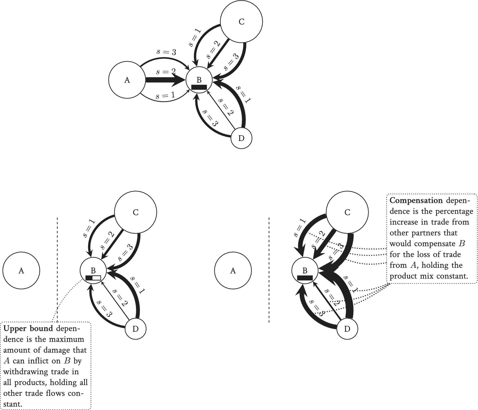


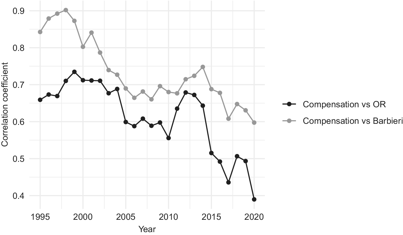
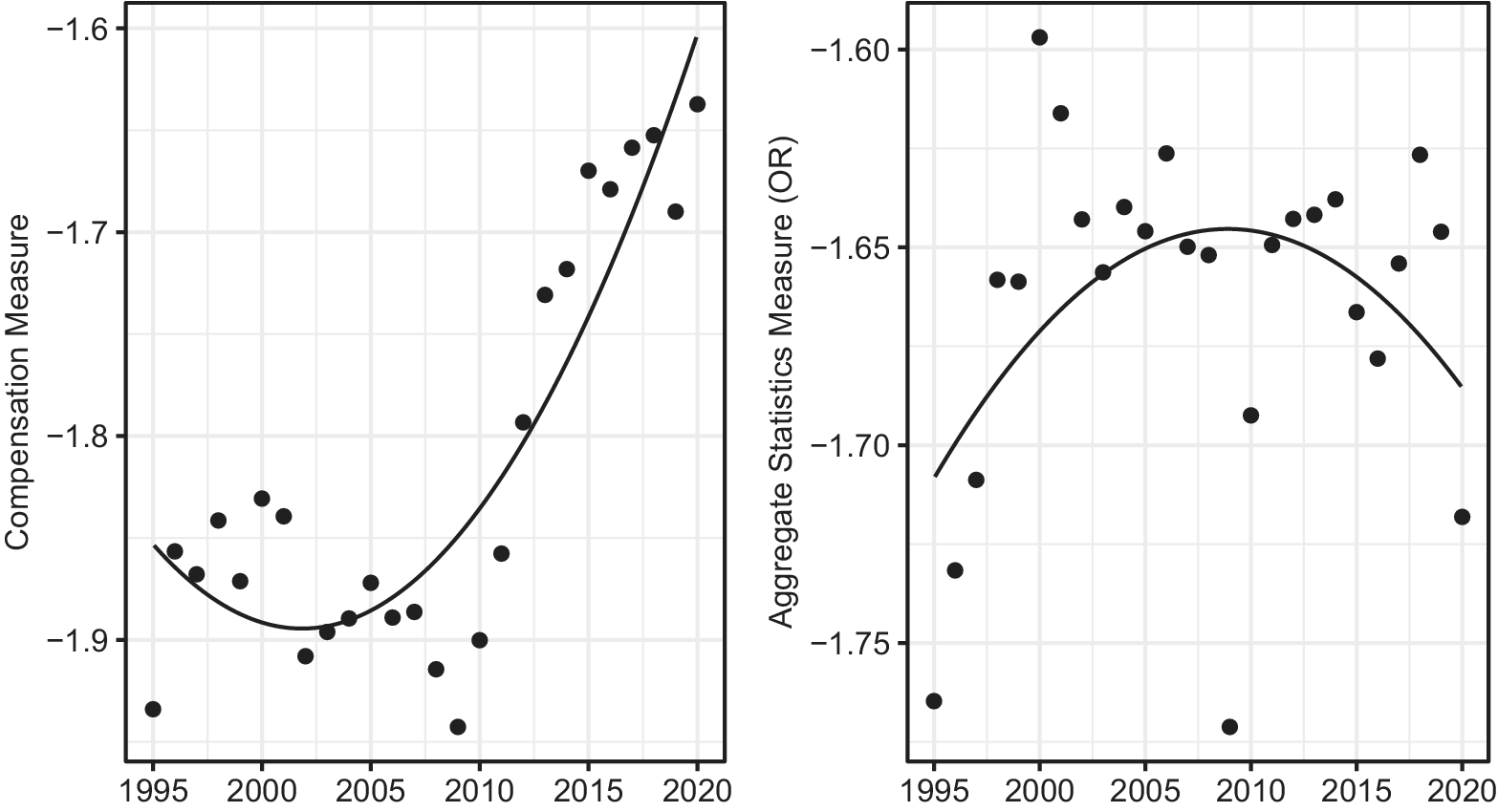


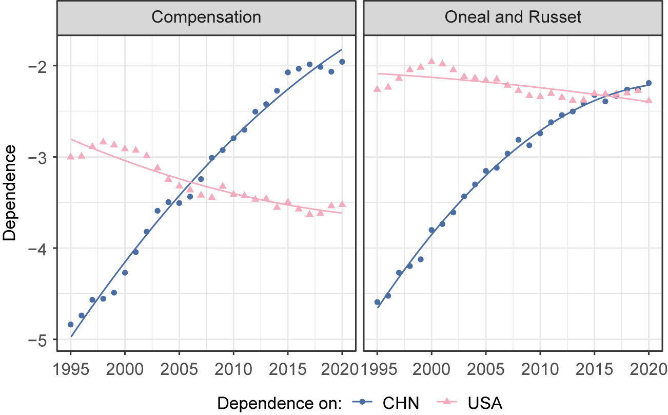

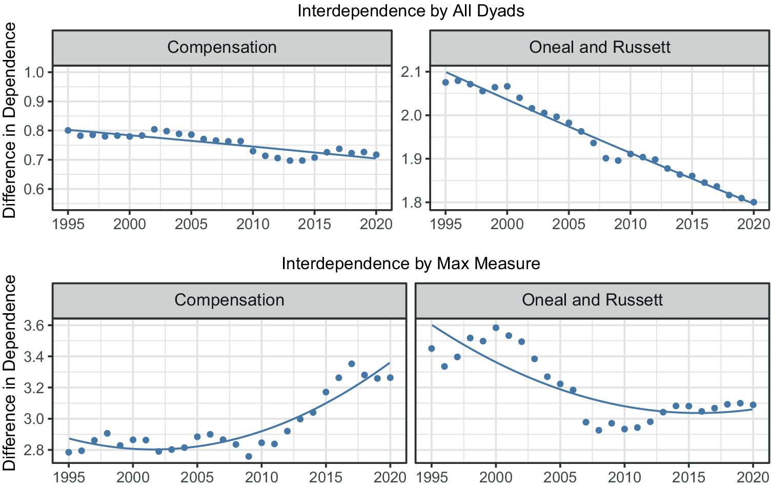
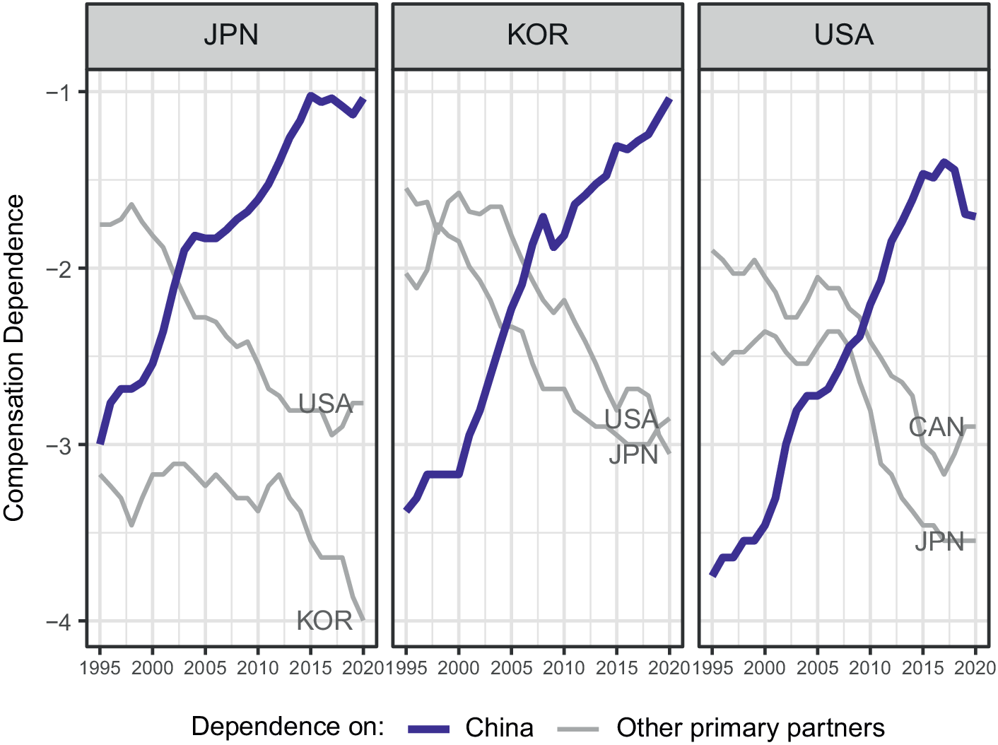
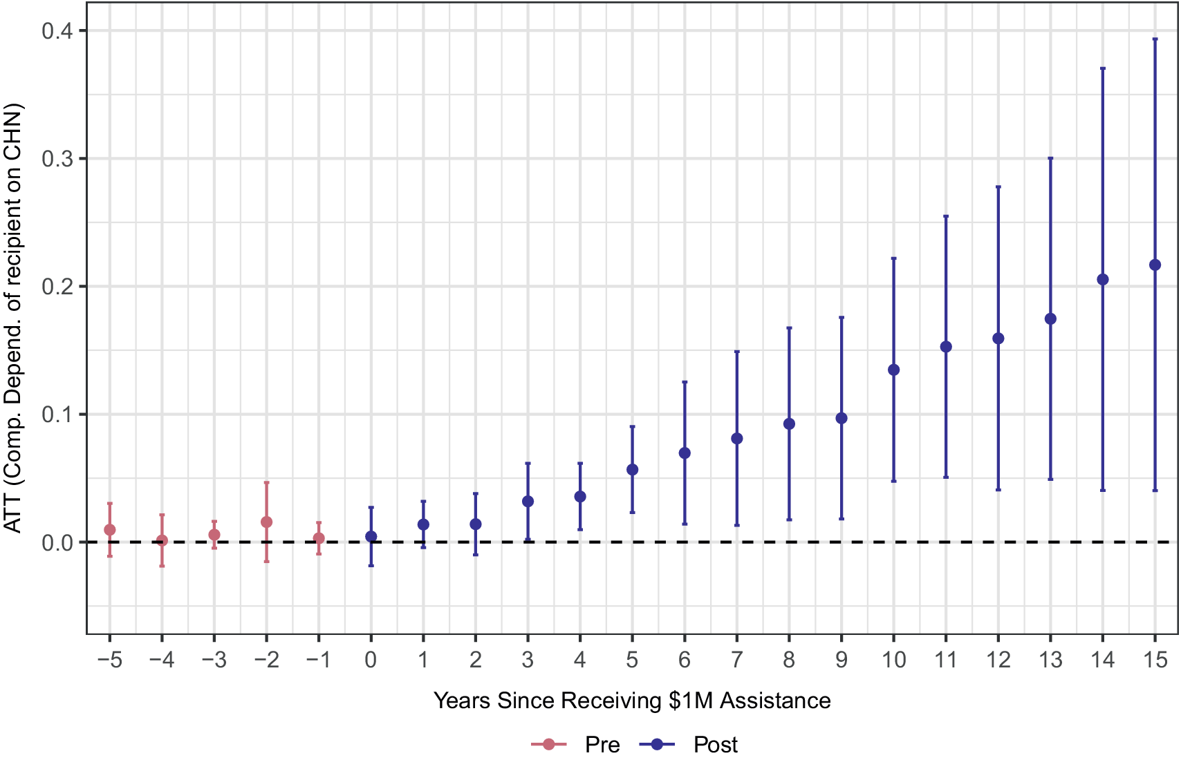
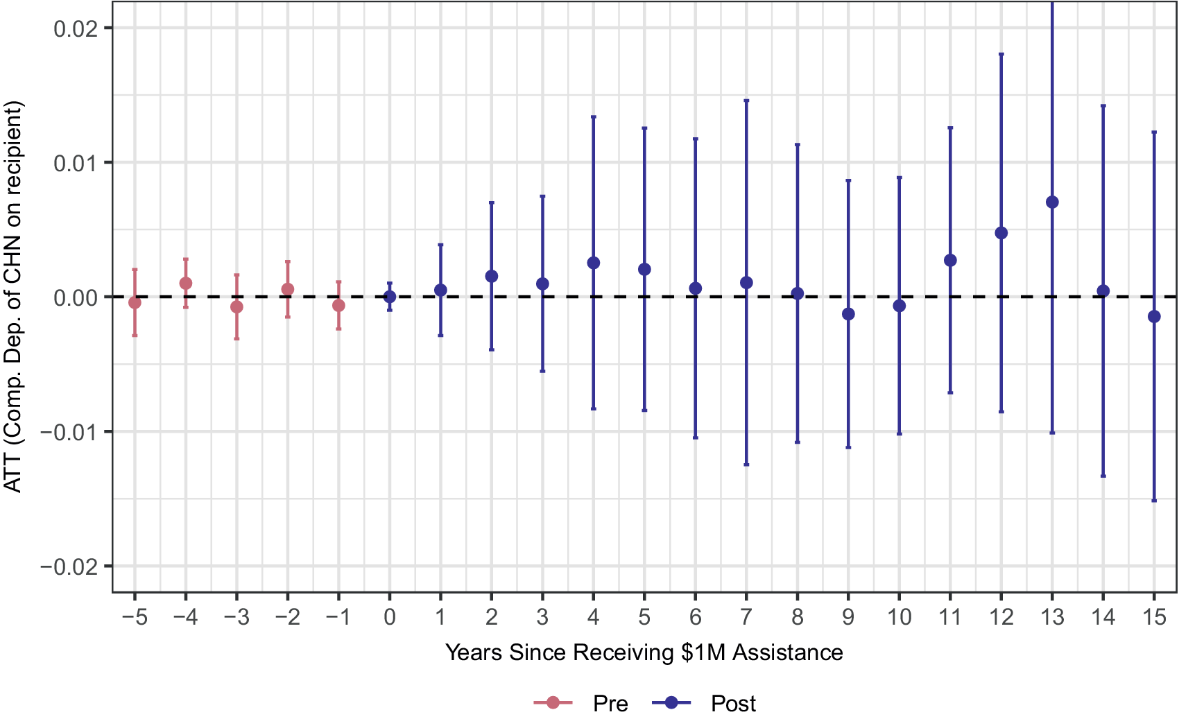
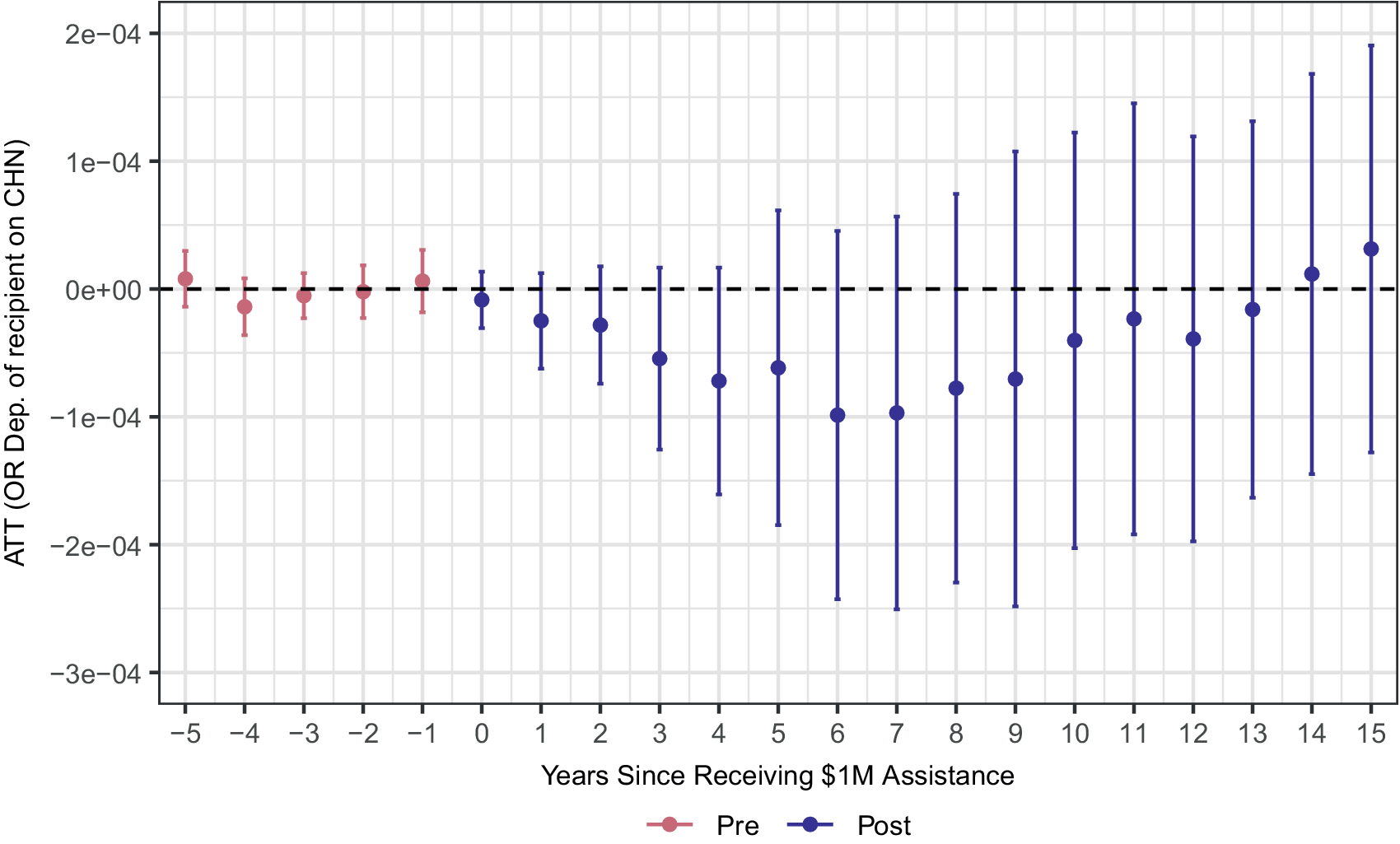




Comments
No Comments have been published for this article.