2.1 Cross-price effects and the inflation rate

Consider a static economy with $n\in \mathbb {N}$ goods produced by a unit mass of firms. The total quantity of each of the $n$ goods produced is given by $x_i^s\geq 0 \,\forall \,i=1,\ldots, n$ , which in turn is supplied in perfectly competitive markets at market prices $p_i\in \mathbb {R}\,\forall \,i=1,\ldots, n$ . We take a short term view and assume that the supply of each good $x_i^s$ is perfectly inelastic with respect to its price $p_i$ . Consumers in turn buy these goods. We consider a unit mass of representative consumers out of which consumer $j$ ’s consumption of the $n$ different types of goods is given by the Walrasian (Marshallian) demand functionFootnote ³ $x_i^{j,d}=x_i^{j,d}(p_i,\boldsymbol{p}_{-i},m^j)$ $\forall \, i=1,\ldots, n$ , with $x_i^{j,d}$ being the quantity demanded of good $i$ , $m^j$ denotes the consumer’s available budget and $\boldsymbol{p}_{-i}=\left [p_k^{ }\right ]_{k=1}^{n \backslash \{i\}} \in \mathbb {R}^{n-1}$ is a vector of prices excluding the price of good $i$ . Summation over the mass of consumers establishes the total demand for good $i$ , which is given by the total demand function $x_i^d= \sum _j x_i^{j,d} = x_i^{d}(p_i,\boldsymbol{p}_{-i}, \sum _j m_j)$ , where the last step follows from the assumption of representative consumers. In equilibrium $x_i^s = x_i^d =x_i$ , which gives rise to the following equilibrium quantity

(1) \begin{equation} x_i=x_i(p_i,\boldsymbol{p}_{-i},m) \end{equation}

where $m=\sum _j m_j$ is consumers’ total income. With the assumption of a perfectly price-inelastic supply, equilibrium prices are shaped by demand shocks only. This implies that, whenever a demand shock occurs, the equilibrium quantity $x_i$ will be left unchanged and only the price $p_i$ will be affected. The latter, though, is likely to shape the demand for yet other goods $x_j\,\forall \,j\neq i$ , which emerges from the circumstance that goods may be substitutes or complements to each other, reflecting consumer preferences. This, in turn, will then also shape the prices of these goods ( $p_j\,\forall \,j\neq i$ ), which establishes links across prices in equilibrium. In what follows, we use this set-up to elaborate on the role of cross-price dependencies for an aggregate price measure and its rate of change. It is useful to this purpose to express the demand function for good $i$ as of equation (1) by means of its inverse demand function $p_i= p_i(x_i,\boldsymbol{p}_{-i})$ . Collecting all goods’ (inverse) total demand functions in the price vector function $\boldsymbol{p}^f(\!\cdot\! )$ gives the following vector of equilibrium prices

(2) \begin{equation} \boldsymbol{p}^f(\boldsymbol{p},\boldsymbol{x})=\left [ \begin{array}{c} p_1(x_1,\boldsymbol{p}_{-1}) \\ \vdots \\ p_n(x_n,\boldsymbol{p}_{-n}) \end{array} \right ] \end{equation}

where all arguments beyond prices $p_i$ are omitted in $p_i(\cdot )$ for simplicity. Letting $\boldsymbol{w} = \left [w_i^{ }\right ]_{i=1}^n$ with $w_i\in [0,1] \, \forall \,i=1,\ldots, n$ and $\sum _{i=1}^nw_i=1$ be the vector of expenditure shares (that is, the weights) of the goods, then the consumer price index $p$ (CPI), as an aggregate price measure, is given by $p=\boldsymbol{w}^{\prime} \boldsymbol{p}^f(\boldsymbol{p},\boldsymbol{x})$ and its change is

(3) \begin{equation} \Delta p=\boldsymbol{w}^{\prime} \cdot \Delta \boldsymbol{p}^f(\boldsymbol{p},\boldsymbol{x}) \end{equation}

where $\boldsymbol{p}=\left [p_i^{ }\right ]_{i=1}^n\in \mathbb {R}^{n}$ and the geometric mean, as used for constructing the CPI (IMF, 2022a), is approximated with the arithmetic mean. Observe that the price vector $\boldsymbol{p}^f(\boldsymbol{p},\boldsymbol{x})$ is a function $\boldsymbol{p}^f:\mathbb {R}^n\rightarrow \mathbb {R}^n$ that takes a vector as input and produces a vector as output. We can identify the cross-price effects from this vector of inverse demand functions by computing the total differential which yields

(4) \begin{equation} \Delta \boldsymbol{p}^f(\boldsymbol{p},\boldsymbol{x}) = \mathcal {A} \cdot \Delta \boldsymbol{p}^f(\boldsymbol{p},\boldsymbol{x}) + \tilde {\boldsymbol{u}} \end{equation}

where $\mathcal {A}=\nabla _{\boldsymbol{p}} \boldsymbol{p}^f(\boldsymbol{p},\boldsymbol{x})$ is a $n\times n$ Jacobian matrix of partial derivatives and given by

(5) \begin{equation} \mathcal {A} = \left [\begin{array}{c@{\quad}c@{\quad}c} 0 & \ldots & \frac {\partial p_1(x_1,\boldsymbol{p}_{-1})}{\partial p_n} \\ & \ddots & \\ \frac {\partial p_n(x_n,\boldsymbol{p}_{-n})}{\partial p_1} & \ldots & 0 \end{array}\right ] \end{equation}

We will henceforth refer to $\mathcal {A}$ as the price-Jacobian matrix. It tells us the relationship between changes in the input and changes in the output, for instance, considering the $i,j$ element, the corresponding entry in $\mathcal {A}$ identifies the effect of a change in $p_j$ on $p_i$ which is given by $\Delta p_i=\frac {\partial p_i(x_i,\boldsymbol{p}_{-i})}{\partial p_j}\cdot \Delta p_j$ . This can be generalized in matrix notation as $\Delta \boldsymbol{p}^f(\boldsymbol{p},\boldsymbol{x}) = \mathcal {A} \cdot \Delta \boldsymbol{p}^f(\boldsymbol{p},\boldsymbol{x})$ . The vector $\tilde {\boldsymbol{u}}=\left [\tilde {u}_1,\ldots, \tilde {u}_n\right ]^{\prime}$ captures demand effects in shaping prices, as for instance, in form of a change in income ( $\nabla _{m} \boldsymbol{p}^f(\boldsymbol{p},\boldsymbol{x})\cdot \Delta m$ ) and alike. In particular, $\tilde {u}_i=\frac {\partial p_i}{\partial m} \Delta m =\frac {\partial p_i}{\partial x_i} \frac {\partial x_i}{\partial m} \Delta m$ , where $\partial p_i/\partial x_i$ determines the slope of the demand curve for good $i$ and $\partial x_i/\partial m$ the slope of the Engel curve. We will henceforth refer to $\tilde {u}_i \in \tilde {\boldsymbol{u}}$ as an exogenous demand shock in the form of a disturbance to the price of good $i$ , so that the own price effect is given by $\Delta p_i=\sum _{j=1}^n\alpha _{ij} \Delta p_j + \tilde {u}_i$ with $\partial p_i(x_i,\boldsymbol{p}_{-i}) / \partial p_j \equiv \alpha _{ij}\in \mathcal {A}$ and the effect on other goods’ prices by $\Delta p_k=\sum _{j=1}^n\alpha _{kj} \Delta p_j \,\forall \,k\neq i$ . Since this relationship has to hold for all prices, it provides a system of equations to solve for all prices in terms of demand shocks $\tilde {\boldsymbol{u}}$ .

Equation (4) solves for the change in the price vector as follows: $\Delta \boldsymbol{p}^f(\boldsymbol{p},\boldsymbol{x}) = (I-\mathcal {A})^{-1}\tilde {\boldsymbol{u}}$ , provided that the inverse of $I-\mathcal {A}$ exists (more on this in Section 2.2). From this equation we can then determine the effect on the CPI inflation rate by using equation (3), which implies

(6) \begin{equation} \pi =\boldsymbol{w}^{\prime} (I-\mathcal {A})^{-1}\boldsymbol{u} \end{equation}

where the CPI inflation rate $\pi$ is given by $\pi =\frac {\Delta p}{p}$ and $\boldsymbol{u}=\tilde {\boldsymbol{u}}/p$ . As equation (6) illustrates, the CPI inflation rate is shaped by cross-price effects captured in the price-Jacobian matrix $\mathcal {A}$ . If the price-Jacobian matrix is equal to the null matrix, then we have that $\partial \pi /\partial u_i=w_i$ , which implies that the effect of a shock to an individual price on the CPI inflation rate equals this price’s weight $w_i$ times the size of the shock. When cross-price dependencies are present, the price-Jacobian matrix is then distinct to the null matrix and a shock to an individual price may affect the CPI inflation rate not only directly, but also via spillover effects arising from the cross-price dependencies. What matters in this context are (i) the sign of the off-diagonal elements in the price-Jacobian matrix $\mathcal {A}$ reflecting the substitution and complementarity relationships among goods, and (ii) the structure that emerges from the cross-price dependencies. In what follows, we discuss this in more detail using graph theory.

2.2 On the price-Jacobian matrix

The price-Jacobian matrix $\mathcal {A}$ in equation (4) is derived under the assumption of inelastic supply. It therefore only captures price effects of demand shocks. We establish equivalent relations to equations (4) and (6) from a supply side approach discussed in the Online Appendix. It is useful to take a closer look at the properties of the price-Jacobian matrix $\mathcal {A}$ and the matrix $\mathcal {L} = (I - \mathcal {A})^{-1}$ . In the context of a production network the latter is commonly referred to as the economy’s Leontief inverse (see the Online Appendix). There economic theory imposes certain restrictions on $(I-\mathcal {A})$ , which guarantee the invertibility of $\mathcal {L}$ and its representation as an infinite sum. While this also applies in our case, the presence of negatively valued edges (due to a substitution relationship among goods) results in a more complex presentation.

First of all, the elements $\alpha _{ij} \in \mathcal {A}$ can have both positive and negative entries. This results from the substitution and complementarity of the goods, reflecting consumer preferences. Consider goods $i$ and $j$ and their prices: a demand shock, for instance, in the form of a change in income $m$ by $dm$ , gives rise to $dx_i=0\, \forall i=1,..,n$ due to the assumption on supply and hence only prices will react: $dp_i/dm=-\frac {dx_i/dm}{dx_i/dp_i}\,\forall i=1,\ldots, n$ . Since $dp_i/dp_j=\frac {dp_i/dm}{dp_j/dm}$ , we obtain the following expression for the cross-price dependencies by means of the total differential of equation (1)

(7) \begin{equation} \frac {\partial p_j}{\partial p_i} = \frac {d x_j/d p_i}{d x_j/d p_j} \lesseqqgtr 0 \end{equation}

Ruling out Giffen goods implies that $d x_j/d p_j \lt 0 \,\forall \, j=1,\ldots, n$ . With regard to cross-price effects, whenever good $i$ and $j$ are complements ( $d x_j/d p_i\lt 0$ ), we have that $\frac {\partial p_j}{\partial p_i}\gt 0$ . Conversely, $\frac {\partial p_j}{\partial p_i}\lt 0$ when they are substitutes. In other words, the demand shock ( $dm$ ) leads to a positive co-movement among prices of those goods that are complements, while the opposite applies to prices of goods that are substitutes.

Second, $\alpha _{ij} \neq \alpha _{ji}$ since in general $\frac {d x_i}{d p_j} \neq \frac {d x_j}{d p_i}$ . This is found in existing empirical studies,Footnote ⁴ moreover, Sethuraman et al. (Reference Sethuraman, Srinivasan and Kim1999) highlight the importance of two effects in this context: the asymmetric price effect and the neighborhood price effect. The asymmetric price effect states that cross-price elasticities are larger when the price changing good has a higher price than the demand changing good. Under the neighborhood price effect, cross-price elasticities are larger when the two competing goods are closer in price.

Third, the price-Jacobian matrix $\mathcal {A}$ captures both own- and cross-price elasticities. Defining by $\varepsilon _{i}=\frac {dx_i/x_i}{dp_i/p_i}$ the (uncompensated) own-price elasticity and by $\varepsilon _{ij}=\frac {dx_i/x_i}{dp_j/p_j}$ the cross-price elasticity of demand, the elements $\alpha _{ij}$ are given by $\alpha _{ij}= \frac {\varepsilon _{ij}}{\varepsilon _i} \frac {p_i}{p_j}$ , and the price-Jacobian matrix can then be decomposed in the following form

(8) \begin{equation} \mathcal {A} = - \boldsymbol{E}^{-1} \bar {\boldsymbol{H}} \end{equation}

where $\boldsymbol{E} =\textrm {diag}\left (|\varepsilon _{i}|,\ldots, |\varepsilon _{n}|\right )$ and $ \bar {\boldsymbol{H}} = [\eta _{ij}]_{ij=1}^n$ with $\eta _{ij}=\varepsilon _{ij}\frac {p_i}{p_j} \lesseqqgtr 0 \,\forall \,i\neq j$ and $\eta _{ij}=0\,\forall \,i=j$ . The matrix $\boldsymbol{E}$ captures the own-price effects while $\bar {\boldsymbol{H}}$ the cross-price demand effects. In what follows, we assume that $\sum _{j=1}^n \varepsilon _{ij} \frac {p_i}{p_j}\lt |\varepsilon _{i}| \,\forall \,i=1,\ldots, n$ . Under this assumption, all column-sums of the price-Jacobian matrix $\mathcal {A}$ are less than unity. This motivates the following Lemma.

Lemma 1. If $\sum _{j=1}^n \varepsilon _{ij}\frac {p_i}{p_j}\lt |\varepsilon _{i}| \,\forall \,i=1,\ldots, n$ , then the matrix $\mathcal {L}$ can be expressed as an infinite sum of the price-Jacobian matrix $\mathcal {A}$ , that is

(9) \begin{equation} \mathcal {L}=(I-\mathcal {A})^{-1} = \sum _{k=0}^{ \infty } \mathcal {A}^k \end{equation}

The proof of Lemma1 follows directly from the relation between any matrix norm and the spectral radius.Footnote ⁵ Important for our context, Lemma1 illustrates that the $(i, j)$ element of the matrix $\mathcal {L}$ , denoted by $l_{ij}$ , captures the importance of price $j$ as a direct and indirect shock transmitter to price $i$ . To see this, note that, for any $i \neq j$ , Lemma1 implies that $l_{ij} = \alpha _{ij} + \sum _{h=1}^n \alpha _{ih}\alpha _{hj}+[\ldots ]$ , with the first term in this expression accounting for price $j$ ’s role as a direct shock transmitter to price $i$ , the second term accounting for price $j$ ’s role as a transmitter to the recipients of price $i$ , and so on. Interpreted in terms of a network, $l_{ij}$ accounts for all possible directed walks that connect price $j$ to price $i$ over the network.

Fourth, in general, most non-zero entries in $\mathcal {A}$ are small in amount as found in existing empirical studies.Footnote ⁶ Moreover, cross-price elasticities enter $\alpha _{ij}\in \mathcal {A}$ only relative to a good’s own price elasticity, which is likely to be larger in amount.

2.3 The price-Jacobian matrix as a graph

The price-Jacobian matrix $\mathcal {A}$ can be considered as a directed weighted graph $\mathcal {G}=(\mathcal {N},\mathcal {E},\mathcal {A})$ , where the $n\gt 1$ nodes in $\mathcal {N}=\{\nu _1,\ldots, \nu _n\}$ represent the goods’ prices $\Delta p_i\, \forall \, i=1,\ldots n$ , which are related to each other via the edges $\mathcal {E}\subseteq \mathcal {N} \times \mathcal {N}$ , and the weight matrix $\mathcal {A} \in \mathbb {R}^{n \times n}_{}$ determines the size (and sign) of the edges. Hence, the elements $\frac {\partial p_i(x_i,\boldsymbol{p}_{-i})}{\partial p_h}$ $\forall \, i,h=1, \ldots, n$ with $i\neq h$ quantify the strength of the network’s edges across nodes $i$ and $h$ , that is, $\nu _i\nu _h \in \mathcal {E} \Longleftrightarrow \frac {\partial p_i(x_i,\boldsymbol{p}_{-i})}{\partial p_h} \neq 0$ with $\frac {\partial p_i(x_i,\boldsymbol{p}_{-i})}{\partial p_h} \in \mathcal {A}$ .

In order to illustrate the role of the network structure for the effects of the cross-price dependencies on the CPI inflation rate, we assume that all non-zero edges have the same weight $\alpha _{ij}=\alpha$ . We further simplify the exposition by considering a graph with three prices ( $n=3$ ), each represented by a node in the network (both assumptions are relaxed in the empirical part). The focus is explicitly on the network’s structure in order to assess its consequence for the inflation rate $\pi$ . To this purpose, we assume that each price has the same weight $w$ in the CPI.

Figure 1.

Examples of network structures.

Note: The table shows distinct network structures and their implications for the spillover effects $\varsigma$ from a shock to the first price by $u_1=1$ . The table also displays the values of three distinct network topology measures (link density (LD), network density (ND) and graph energy (GE $_{\mathbb {R}}$ )) for each network structure. For $\alpha =1$ , we have that GE $_{\mathbb {R}}=$ GE $_{\mathbb {Z}_2}$ .

Figure 1 shows several simple network structures (first column) and their consequences for the CPI inflation rate in response to a shock in the first price ( $u_1$ ). We establish the adjacency matrix $\mathcal {A}$ for the five cases, (a)–(e), and compute the CPI inflation rate $\pi$ using equation (6). In the absence of links, the effect of a unit-shock to the first price ( $u_1=1$ ) on the CPI inflation rate equals $\pi ^{(a)}=w$ (the superscript “(a)” refers to the case considered). Hence the effect of the shock ( $u_1$ ) on the CPI inflation rate equals the weight $w$ of the first price times the size of the shock. We refer to this case as the “zero-link” case and it is given by $\pi ^{(a)}=\boldsymbol{w}^{\prime}\boldsymbol{u}$ in a more general form. The introduction of links between the prices extends the zero-link effects by spillover effects ( $\varsigma$ ), that is, the effects relative to those emanating from the zero-link case (a):

(10) \begin{eqnarray} \varsigma ^{(i)}&=&\pi ^{(i)}-\pi ^{(a)} \nonumber \\ &=& \boldsymbol{w}^{\prime} (I-\mathcal {A})^{-1}\boldsymbol{u} - \boldsymbol{w}^{\prime}\boldsymbol{u} \nonumber \\ &=&\boldsymbol{w}^{\prime} \left ((I-\mathcal {A})^{-1}- I\right ) \boldsymbol{u} \end{eqnarray}

Importantly, the spillover effects (second column in Figure 1) emerge from the cross-price dependencies, and they reflect the degree of connectedness in the network. The degree of connectedness is in turn shaped by (i) a strength effect and (ii) a diffusion effect. When no links are present, the price-Jacobian matrix is equal to the null matrix. Hence, the spillover effects are equal to zero as neither a strength nor a diffusion effect applies. When the goods are complements to each other ( $\alpha \gt 0$ ), then the strength effect implies that the degree of connectedness (and hence the spillover effects) increases with $\alpha$ , as can be seen in case (b): $\partial \varsigma ^{(b)}/\partial \alpha =w\gt 0$ . Conversely, the diffusion effect implies that the degree of connectedness (and hence the spillover effects) is determined by the number of links ( $\varsigma ^{(b)}\lt \varsigma ^{(c)}\lt \varsigma ^{(d)}$ ) and by the structure of the links in directed networksFootnote ⁷ (acyclic or cyclic network structures: $\varsigma ^{(d)}\lt \varsigma ^{(e)}$ when $\alpha \in (0,1)$ ).

A complication arises from the fact that goods may be substitutes to each other ( $\alpha \lt 0$ ). Considering case (c), we then have that $\partial \varsigma ^{(c)}/\partial \alpha =w+2w\alpha \gtreqqless 0$ , which implies that for certain network structures, the strength (and diffusion) effect can go either way.

The network structure is typically captured by so called network topology measures. The challenge in this respect is to establish network topology measures that adequately capture the variation in the spillover effects due to distinct network structures and edge weights $\alpha$ . In what follows, we introduce three distinct network topology measures to capture the spillover effects.

2.4 Network topology measures and spillover effects

We use network topology measures to capture the size and the sign of the spillover effects, paying attention to strength and diffusion effect. The former concerns the quantitative size of the link between two connected nodes, while the latter concerns the amount of links and the overall arrangement of the links. We consider the following network topology measures:

1. 1. Link density (LD): This measures how many links exist between nodes relative to the maximum possible number of links (Newman, Reference Newman2010). Link density is thus a measure for the diffusion effect. For a directed graph with an $N\times N$ adjacency matrix $B=[\beta _{ij}]_{ij=1,\ldots, N}$ with $B\neq B^{\prime}$ , the link density is given by the scalar $\textrm {LD}(B)=\frac {\sum _i^N \sum _{j\neq i}^N\unicode {x1D7D9}_{ \{|\beta _{ij}|\gt 0 \}}}{N(N-1)}\in [0,1]$ , where $N$ is the number of nodesFootnote ⁸ and $\unicode {x1D7D9}_{\{ |\beta _{ij}|\gt 0 \}}$ is the indicator function, which takes on a value of one if the condition $|\beta _{ij}|\gt 0$ is satisfied.

2. 2. Network density (ND): For the same directed graph as before, the network density (Horvath, Reference Horvath2011) is given by the scalar $\textrm {ND}(B) =\frac {\sum _i^N \sum _{j\neq i}^N \beta _{ij}}{N(N-1)} \in \mathbb {R}$ . It extends the link density by taking into account the weight of each edge $\beta _{ij}\in B$ . Thus, for a given link density, the network density measures the strength effect.

3. 3. Graph energy (GE): For the same graph as before, the graph energy is defined by the scalar $\textrm {GE}(B) = \sum _{i=1}^N |\mathfrak {R}(z_i)|$ , where $\mathfrak {R}(z_i)$ is the real part of the complex number $z_i$ , and the $z_i\,\forall \,i=1,\ldots, N$ are the eigenvalues of the adjacency matrix $B$ (Gutman, Reference Gutman1978; Peña and Rada, Reference Peña and Rada2008). $GE(B)=0$ means that a network has a perfect tree-like structure in which no loop is formed. Thus, the higher the graph energy,Footnote ⁹ the more cyclic is the architecture of the network. We consider two versions of graph energy: the first is given by GE $_{\mathbb {Z}_2}\geq 0$ (henceforth binary GE) and is based on $\beta _{ij}\in B$ with $\beta _{ij}\in \{0,1\}\,\forall \, i,j=1,\ldots, N$ and $i\neq j$ , and the second is given by GE $_{\mathbb {R}} \geq 0$ (henceforth non-binary GE) and is based on $\beta _{ij}\in B$ with $\beta _{ij}\in \mathbb {R}\,\forall \, i,j=1,\ldots, N$ and $i\neq j$ . The first measure (GE $_{\mathbb {Z}_2}$ ) captures the diffusion effect solely, while the second (GE $_{\mathbb {R}}$ ) captures both the diffusion and the strength effect.

We show the values of the three network topology measures for each of the five cases (a)–(e) in the third to fifth columns of Figure 1. Their adequacy for our analysis is determined by their ability to capture the size and sign of the spillover effects.

Considering Figure 1, in the absence of links, no spillover effects arise ( $\varsigma ^{(a)}=0$ ) and the three topology measures (LD, ND, and GE) are all equal to zero. When links are present, spillover effects occur. Whenever the goods are complements ( $\alpha \gt 0$ ), increasing the number of links leads to yet larger spillover effects (second column) due to the diffusion effect. This is captured by the link density (third column) and applies to the cases (b)–(d). However, for the same cases, the presence of substitutes ( $\alpha \lt 0$ ) renders the spillover effects negative, thus mitigating the effects of the shock. While the link density fails to capture this, the network density in turn does (fourth column), as it captures the strength effect, which in turn is affected by the sign of the edges. Importantly, though, a positive spillover effect can also occur in the case of substitutes. This is indicated by cases (c) and (d) and is shown in Figure 2, which illustrates the spillover effects for varying edge weights $\alpha$ .

Figure 2.

Spillover effects and inflation.

Note: Panel (a) shows the spillover effects of a unit-shock to the first node ( $u_1=1$ ) for varying values of the edge weight $\alpha$ for a given node weight $w=1/3$ . Panel (b) shows the volatility of the CPI inflation rate as a function of the number of prices (nodes, $n$ ) in the network (each price $i$ has a weight $w_i=1/n$ in the CPI) for three distinct values of the edge weight $\alpha$ .

Finally, case (e) comprises an interesting alternative network structure. It shares similarities with cases (c) and (d). The similarity with case (c) emerges from the fact that the CPI inflation rate for the network structure in case (c) is given by

(11) \begin{equation} \pi ^{(c)}=\frac {w}{1-\alpha } \end{equation}

and the spillover effect by $\varsigma ^{(c)}=\frac {w\alpha }{1-\alpha }$ once the number of nodes $n$ becomes large and each node (except the first and the last) has exactly one in-degree and one out-degree,Footnote ¹⁰ and $|\alpha |\lt 1$ . In this case, the two networks have the same spillover effects despite their distinct structures. In contrast, as regards cases (d) and (e), while the link and network densities are the same for these two cases, the graph energy is not. In particular, the spillover effect arising from case (e) can indeed be sizeable, especially in the case of complementsFootnote ¹¹ (see Figure 2). Hence, the link and network density fail to capture this effect adequately from a quantitative point of view. Importantly, the effect emerges from a cyclical feature: Cases (b)–(d) represent acyclic networks, each with a nilpotent adjacency matrix. Case (e), on the other hand, is a cyclic network, which differs from the previous ones in that once a shock hits this network, a series of knock-on effects arise from the fact that the shock is continuously transmitted through the nodes forming the cycle (Boccaletti et al. Reference Boccaletti, Latora, Moreno, Chavez and Hwang2006). From a technical point of view, the adjacency matrix has non-zero eigenvalues (Newman, Reference Newman2010). While the number of non-zero eigenvalues depends on the number of cycles present in the network, we hence use an overall eigenvalue measure, which is given by the graph energy.Footnote ¹² This measure captures spillover effects emerging from cycles.

2.5 Individual price shocks and inflation dynamics

While the previous section illustrated the extent to which cross-price dependencies can act as a mechanism for propagating shocks from one good’s price to the CPI inflation rate, we now examine whether they play a role for the inflation volatility.

Using equation (6) and setting the price-Jacobian matrix $\mathcal {A}$ equal to the null matrix (case (a) of Figure 1) implies that the volatility of the CPI inflation rate $\pi$ that is due to idiosyncratic microeconomic price shocks is given by

(12) \begin{equation} \sigma (\pi )^{(a)} = ||\boldsymbol{w}|| \end{equation}

where $\sigma (\cdot )$ denotes the standard deviation and the demand shocks’ variance is given by $E[\boldsymbol{u}\boldsymbol{u}^{\prime}]=I$ . Since $||\boldsymbol{w}||=(\sum _{i=1}^n w_i^2)^{1/2}$ , equation (12) highlights that more dispersion in the weights $\boldsymbol{w}$ can result in higher levels of volatility emerging from purely idiosyncratic shocks. In this regards, Gelos and Ustyugova (Reference Gelos and Ustyugova2017) highlight that countries with a higher weight of food in the CPI experience more persistent inflationary effects from commodity price shocks. In the absence of dispersion in the weights ( $w_i=w \, \forall \, i = 1, \ldots, n$ ), we have that

(13) \begin{equation} \sigma (\pi )^{(a)}= \frac {1}{\sqrt {n}} \end{equation}

since the weights $\boldsymbol{w}$ satisfy $\sum _{i=1}^{n}w_i=1=nw$ . This equation implies that when the weights of all prices are identical, the volatility of the inflation rate is proportional to $1/\sqrt {n}$ , which is consistent with the diversification argument put forth in the context of production networksFootnote ¹³ (Acemoglu et al. Reference Acemoglu, Carvalho, Ozdaglar and Tahbaz-Salehi2012; Fadinger et al. Reference Fadinger, Ghiglino and Teteryatnikova2022) and financial networks (Teteryatnikova, Reference Teteryatnikova2014; Glasserman and Young, Reference Glasserman and Young2016; Das et al. Reference Das, Kalimipalli and Nayak2022; Balcilar et al. Reference Balcilar, Elsayed and Hammoudeh2023). However, the presence of cross-price dependencies can render the effects of a shock from any individual price large, irrespective of the dispersion of the weights. In this case, the prices of goods would be correlated, and thus individual price shocks may not disappear when aggregated, even if the shocks themselves are independent. Consider case (c) of Figure 1, where $|\alpha |\lt 1$ and $n$ is large; the effect of a shock to $u_1$ on the CPI inflation rate is given in equation (11); generalizing this result to the vector of shocks $\boldsymbol{u}$ , we then obtain the following

(14) \begin{equation} \sigma (\pi )^{(c)}=\frac {1}{(1-\alpha )\sqrt {n}} \end{equation}

which implies that $\sigma (\pi )^{(c)}\gt \sigma (\pi )^{(a)}$ whenever $\alpha \gt 0$ due to network spillover effects. The above equation highlights that there is a tradeoff between the network and the volatility of the CPI inflation rate: A higher degree of connectedness–either via the strength effect (higher value of $|\alpha |$ ) and/or the diffusion effect (larger number of connections)–exacerbates the effect of microeconomic price shocks on the CPI inflation rate. The effect rises with a low number of nodes $n$ , but then quickly gets attenuated by the degree of diversification, that is, a high $n$ . This argument, however, only holds when cross-price dependencies emerge in the wake of complements ( $\alpha \gt 0$ ), as illustrated in panel (b) of Figure 2. When dependencies arise from substitutes, then both the network effect (higher or lower degree of connectedness) and the diversification effect operate in the same direction rendering the mitigation of microeconomic shocks especially strong. In other words, each shock dissipates quickly and exerts an effect on the CPI inflation rate that is smaller than its pure DE.

3.1 The econometric methodology

Our objective is to estimate demand-driven cross-price dependencies in a setting where, unlike the theoretical model presented in Section 2, supply is not perfectly price inelastic. To achieve this, we employ a vector autoregressive (VAR) model and sequentially estimate the components of the price-Jacobian matrix $\mathcal {A}$ , as defined in equation (4).

We define the vector of endogenous variables as $\mathbf {y}_t^{ij} = \left [x_t^i, x_t^j, p_t^i, p_t^j\right ]^{\prime}$ , where $x_t^i,x_t^j$ denote the (equilibrium) quantities and $p_t^i,p_t^j$ the (equilibrium) prices of goods $i$ and $j$ , while $\mathbf {x}_{t-1}$ represents a ( $k \times 1$ ) vector (with $k = 4m + 1$ ), comprising a constant and $m$ lags of $\mathbf {y}$ , denoted as $\mathbf {x}_{t-1}=\left [(\mathbf {y}_{t-1}^{ij})^{\prime}, \dots, (\mathbf {y}_{t-m}^{ij})^{\prime}, \mathbf {1}^{\prime}\right ]^{\prime}$ . Furthermore, $\mathbf {u}_t$ is a ( $4 \times 1$ ) vector of structural disturbances with a diagonal variance-covariance matrix denoted by $\mathbf {I}$ (idenity matrix). The structural VAR model is thus expressed as (for clarity and brevity, the $ij$ superscript is omitted from all elements except $\mathbf {y}_t^{ij}$ )

(15) \begin{equation} \mathbf {A}\mathbf {y}_t^{ij} = \mathbf {B}\mathbf {x}_{t-1} + \mathbf {u}_t \end{equation}

To quantify demand-driven cross-price dependencies, we proceed by considering the following structural model, which is comprised by a system of supply (S) and demand (D) equations for goods $i$ and $j$

(16) \begin{align} \textrm {S}_i:\quad x_t^i&=\gamma _i p_t^i + \gamma _{ij} p_t^j + \zeta _{ij}x_t^j+\mathbf {b}_1^{\prime}\mathbf {x}_{t-1}+u_{S,t}^i \quad \textrm {with}\, \gamma _i\gt 0 \end{align}

(17) \begin{align} \textrm {S}_j:\quad x_t^j&=\gamma _j p_t^j + \gamma _{ji} p_t^i + \zeta _{ji}x_t^i+\mathbf {b}_2^{\prime}\mathbf {x}_{t-1}+u_{S,t}^j \quad \textrm {with}\, \gamma _j\gt 0 \end{align}

(18) \begin{align} \textrm {D}_i:\quad p_t^i&=a_i x_t^i + a_{ij} p_t^j + \xi _{ij}x_t^j+\mathbf {b}_3^{\prime}\mathbf {x}_{t-1}+u_{D,t}^i \quad \textrm {with}\, a_i\lt 0 \end{align}

(19) \begin{align} \textrm {D}_j:\quad p_t^j&=a_j x_t^j + a_{ji} p_t^i + \xi _{ji}x_t^i+\mathbf {b}_4^{\prime}\mathbf {x}_{t-1}+u_{D,t}^j \quad \textrm {with}\, a_j\lt 0\\[12pt]\nonumber \end{align}

In the two supply curves, $\gamma _i\gt 0$ and $\gamma _j\gt 0$ are the short-run price elasticities of supply. The two demand curves are written in inverse form, so that $a_i\lt 0$ and $a_j\lt 0$ (we rule out Giffen goods) are hence the reciprocal of the price elasticities of demand. Our focus is on the cross-price elasticities $a_{ij}$ and $a_{ji}$ , which we intend to estimate. In view of equation (7) and the two (inverse) demand equations (18) and (19), we have that the demand-driven cross-price dependencies are given by

(20) \begin{equation} \frac {\partial p_t^j}{\partial p_t^i} = \frac {d x_t^j/d p_t^i}{d x_t^j/d p_t^j} = \frac {-a_{ji}/a_j}{1/a_j}=-a_{ji} \end{equation}

so that $-a_{ji}\lt 0$ implies substitutes and $-a_{ji}\gt 0$ complements. We use these estimates to populate the price-Jacobian matrix $-a_{ji} \in \mathcal {A}$ sequentially.Footnote ¹⁶ To this purpose, we reformulate the above system of equations (16)–(19) into the structural VAR model (15), where the matrix $\mathbf {A}$ , governing the contemporaneous interactions among the endogenous variables, is given by

(21) \begin{equation} \mathbf {A}=\left [ \begin{array}{cccc} 1 & \boldsymbol {\cdot } & -\gamma _i & \boldsymbol {\cdot } \\ \boldsymbol {\cdot } &1 & \boldsymbol {\cdot } & -\gamma _j \\ -a_i & \boldsymbol {\cdot } & 1 & -a_{ij} \\ \boldsymbol {\cdot } & -a_j & -a_{ji} & 1 \end{array}\right ] \end{equation}

All parameters of the contemporaneous relationship beyond interest were substituted with a dot. The structural model (15) has the following reduced form representation

(22) \begin{align} \mathbf{y}_t^{ij} &= \boldsymbol{\Phi } \mathbf {x}_{t-1} + \boldsymbol{\epsilon }_t\end{align}

(23) \begin{align} \boldsymbol {\epsilon }_t&=\mathbf {H} \mathbf {u}_t \\[9pt]\nonumber\end{align}

where $\mathbf {H}=\mathbf {A}^{-1}$ , $\boldsymbol {\Phi }=\mathbf {A}^{-1}\mathbf {B}$ and $E(\boldsymbol {\epsilon }_t\boldsymbol {\epsilon }_t^{\prime})=\boldsymbol{\Sigma }$ , with $\boldsymbol {\epsilon }_t$ being the reduced form error term. We estimate the reduced form model using Bayesian techniques (consider the Online Appendix for further technical details) and we use the Schwarz (Bayesian) information criterion to select the lag length. The variables $p_t^i$ and $p_t^j\, \forall \, i,j=1,\ldots, n$ refer to the three-digit level subindices of the CPI and they enter the vector $\mathbf {y}_t^{ij}$ in annual percentage changes. The quantities ( $x_t^i$ and $x_t^j$ ) are taken from national account consumption data and they also enter in annual percentage changes. Importantly, they have the same COICOP classification as the CPI, and hence correspond directly to the respective prices ( $ p_t^i$ and $p_t^j$ ).Footnote ¹⁷ Additionally we use two dummy variables, one of which for the Covid-19 episode and the second for the post-pandemic episode. These variables are used for each country. The monthly dataset spans from January 2000 to December 2023,Footnote ¹⁸ yielding a total of $T=288$ observations. We estimate equation (22) for each pairing $i,j$ of prices and quantities and for each country individually, so that each individual VAR provides estimates for two entries in the price-Jacobian matrix $\mathcal {A}$ . With $n=39$ , this requires to estimate $n(n-1)/2=741$ models in total for each of the 28 countries.

3.1.1 Identification

An important element of our empirical approach concerns the identification of the structural equation system (16)–(19), that is, the transformation of the reduced form VAR model (22) into the structural form (15). To this purpose, we employ sign restrictions. However, in contrast to the literature (see among others Canova and De Nicolo Reference Canova and De Nicolo2002; Uhlig, Reference Uhlig2005; Baumeister and Peersman, Reference Baumeister and Peersman2013; Glocker and Towbin, Reference Glocker and Towbin2015), we do not consider sign restrictions on the impulse response functions, but on the elements in the matrix $\mathbf {A}$ . In view of the structural equation system (16)–(19), we expect the following signs of the elements in the matrix $\mathbf {A}$

(24) \begin{equation} \textrm {sign}{(\mathbf {A})}= \left [ \begin{array}{cccc} + & \boldsymbol {\cdot } & - & \boldsymbol {\cdot } \\ \boldsymbol {\cdot } &+ & \boldsymbol {\cdot } & - \\ + & \boldsymbol {\cdot } & + & \boldsymbol {\cdot } \\ \boldsymbol {\cdot } & + & \boldsymbol {\cdot } & + \end{array}\right ] \end{equation}

where a dot refers to an unrestricted element. The “ $+$ ” and “ $-$ ” symbols refer to the sign restrictions that we impose. Importantly, we leave the two demand-driven cross-price elasticities $a_{ji}$ (the [3,4]-element) and $a_{ij}$ (the [4,3]-element) unrestricted as we intend to be agnostic about their sign (and size).

We use the eigenvector-eigenvalue decomposition of the variance-covariance matrix $\boldsymbol{\Sigma }$ and define $\mathbf {V}=\mathbf {E}_{\boldsymbol{\Sigma }}\boldsymbol{\Lambda}_{\boldsymbol{\Sigma }}^{1/2}$ , where $\mathbf {E}_{\boldsymbol{\Sigma }}$ is the (orthogonal) matrix of eigenvectors and $\boldsymbol{\Lambda}_{\boldsymbol{\Sigma }}$ is the (diagonal) matrix of eigenvalues. In view of the properties of this decomposition in case of symmetric matrices ( $\mathbf {E}_{\boldsymbol{\Sigma }}^{\prime}=\mathbf {E}_{\boldsymbol{\Sigma }}^{-1}$ , since $\mathbf {E}_{\boldsymbol{\Sigma }}$ is an orthogonal matrix), we have that $\boldsymbol{\Sigma }=\mathbf {V}\mathbf {V}^{\prime}$ . We then multiply $\mathbf {V}$ with an orthonormal matrix $\mathbf {Q}$ to obtain $\mathbf {H}=\mathbf {V}\mathbf {Q}$ , from which we can compute a candidate for $\mathbf {A}=\mathbf {H}^{-1}$ . The matrix $\mathbf {Q}$ is a random orthonormal matrix of the same dimension as $\boldsymbol{\Sigma }$ . We follow Rubio-Ramírez et al. (Reference Rubio-Ramírez, Waggoner and Zha2010) and compute $\mathbf {Q}$ by drawing an independent standard normal matrix $\mathbf {X}$ (of the same size as $\boldsymbol{\Sigma }$ ) and apply the QR decomposition $\mathbf {X}=\mathbf {Q}\mathbf {R}$ to get $\mathbf {Q}$ .

Regarding the sign restrictions, if the corresponding entries in a candidate matrix $\mathbf {A}$ are consistent with the sign restrictions outlined in (24), we retain the candidate draw and proceed to the next draw until a total of 5,000 accepted draws is obtained. Otherwise, a new $\mathbf {Q}$ matrix is drawn until the sign restrictions are satisfied.

Notably, we impose two additional constraints: (i) simultaneous supply shocks are prohibited, which excludes rows of the form $[+,+,-,-]$ in the first and second rows of $\mathbf {A}$ ; and (ii) simultaneous demand shocks are also prohibited, excluding rows of the form $[+,+,+,+]$ in the third and fourth rows of $\mathbf {A}$ . These additional restrictions ensure that neither aggregate supply nor aggregate demand shocks influence the individual good-specific relationships.

We emphasize that while the estimation and inference of the reduced-form model are based on a fairly non-informative prior for all coefficients, an informative prior arises in the structural model due to the QR decomposition (Baumeister and Hamilton, Reference Baumeister and Hamilton2015). Additionally, it is important to note that in our case, the sign restrictions are applied row-wise to the matrix $\mathbf {A}$ . This differs from the column-wise procedure used for the matrix $\mathbf {H}$ when applying sign restrictions to impulse response functions following structural shocks (see for example Baumeister & Hamilton, Reference Baumeister and Hamilton2015, Reference Baumeister and Hamilton2019).

We consider two alternative approaches to identification, both of which are described in detail in the Online Appendix and serve as robustness checks. The first approach involves sign restrictions on the impulse response functions and hence on the columns of the matrix $\mathbf {H}$ . The advantage of this alternative approach is that it allows for the inclusion of lags in the effects associated with demand-driven cross-price dependencies. The second approach considers a combination of sign and size restrictions, applied on the rows of the matrix $\mathbf {A}$ . The size restrictions set the elasticity for a good with respect to its own price relative to that of another price. This introduces Lemma1 into the empirical model. While the size restrictions we impose are slightly different from the one in Lemma1, they are still closely related, since in both cases the own-price elasticity is set relative to the cross-price elasticity.Footnote ¹⁹

3.1.2 In-significant entries

We use the posterior median for the $a_{ij}$ elements. In many cases, the estimated values of $a_{ij}$ are small and statistically indistinguishable from zero. To address this, we introduce an additional step involving statistical inference. We transform the estimated matrix $\mathcal {A}$ that emerges from the repeated estimation of equation (15) into an adjacency matrix $\tilde {\mathcal {A}}$ by applying the following statistical thresholding

(25) \begin{eqnarray} \tilde {\alpha }_{ij} = \begin{cases} a_{ij} & \textrm {if} \, \forall \, i \neq j: \, \textrm {Pr}( a_{ij} \neq 0) \geq 1-\bar {p} \\ 0 & \textrm {else} \end{cases} \end{eqnarray}

where $-a_{ij}\in \mathcal {A}$ and $-\tilde { \alpha }_{ij} \in \tilde {\mathcal {A}}$ , and we use a significance value of $\bar {p}$ equal to one percent. In other words, all elements in the price-Jacobian matrix ( $\tilde {\alpha }_{ij}$ ), for which the corresponding values of the $a_{ij}$ elements are not statistically different from zero, are set to zero. The $\tilde {\alpha }_{ij}$ elements then define the edges of the weighted directed network of empirical cross-price dependencies. Since we have a posterior distribution for $\mathcal {A}$ , the same then applies to the adjacency matrix $\tilde {\mathcal {A}}$ (in particular, its non-zero elements). Moreover, we keep all those posterior draws of $\tilde {\mathcal {A}}$ that satisfy Lemma1. On average (across countries), three percent of the draws are discarded as a consequence.Footnote ²⁰

3.2 The empirical demand-driven cross-price dependencies

Figure 3.

Demand driven cross-price dependencies.

Note: The figure shows the cross-price dependencies as a network. We only show the edges that are present in 50 percent of the countries. Nodes in red indicate out-degree dominance, while those in green indicate in-degree dominance; nodes in blue indicate equality between out- and in-degree. Edges in red refer to positive valued links (complements) and those in black to negative ones (substitutes). The network shown is the average over all countries (the UK and the current EU member countries). The key nodes are: (1) “Food,” (3) “Alcoholic Beverages,” (4) “Tobacco,” (5) “Clothing,” (6) “Footwear,” (7) “Actual Rentals for Housing,” (8) “Maintenance and Repair of the Dwelling,” (13) “Household Appliances,” (14) “Glassware, Tableware and Household Utensils,” (15) “Tools and Equipment for House and Garden,” (19) “Hospital Services,” (21) “Operation of Personal Transport Equipment,” (22) “Transport Services,” (25) “Telephone and Telefax Equipment,” (31) “Package Holidays,” (32) “Catering Services,” (33) “Accommodation Services,” and (39) “Other services.”

Figure 3 shows the empirical cross-price dependencies given by the matrix $\tilde {\mathcal {A}}$ across all countries. We display only those edges that are present in 50 percent of the countries, in order to allow for a reasonable inspection of the most relevant links. Edges in red refer to positive entries (complements) and those in black to negative ones (substitutes).

The estimated cross-price dependencies imply, for instance, that an increase in demand for food (node 1) leads to higher prices in this group and to price changes in two closely related groups, that is, alcoholic beverages (node 3) and tobacco (node 4), both of which are affected positively, highlighting complementary effects. Food prices are connected with the prices of catering services (node 32), which also affect the prices of other goods.

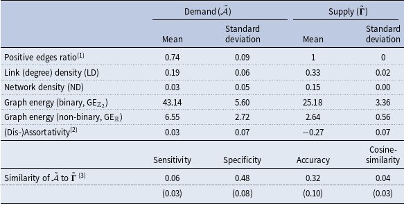
As a second example, consider an increase in rental prices for housing (node 7), which triggers substitution effects for tobacco (node 4) and clothing (node 6). The latter, in turn, forms a cycle with footwear (node 5), that is, higher demand for clothing raises demand for footwear with price increases in both groups; higher demand for footwear in turn stimulates demand for clothing with another round of price increases in both groups. The interaction is shaped by positive-valued edges resulting in goods being complementary to each other. Table 1 highlights that the complementarity property of goods dominates. The mean (across countries) of the ratio of positive-valued edges to the total number of non-zero edges equals 74 percent, which is well in line with the 67 percent estimate in Regmi and Seale (Reference Regmi and Seale2010). A cross-country mean value of 19 percent for the link (degree) density contrasts a fairly low value for the network density due to negative-valued edges.

Table 1.

Network topology statistics

Notes: The moments (Mean and Standard deviation) are computed for each network topology measure across the countries. The figures shown are the mean and the standard deviation (in parenthesis in the lower part of the Table) across the countries. ⁽¹⁾ Positive edges ratio denotes the number of edges with a positive value relative to the total number of non-zero edges.⁽²⁾ Assortativity (Dis-assortativity if negative) is a measure of the preference of nodes in a network to attach to others that are (dis-)similar in terms of their degree. It is operationalized as the correlation between two nodes. ⁽³⁾ $\skew{5}\tilde {\mathcal {A}}$ refers to the demand-driven and $\tilde {\boldsymbol {\Gamma }}$ to the supply-driven network of cross-price dependencies.

3.3 Demand and supply-driven cross-price dependencies: a comparison

Figure 4.

Supply driven cross-price dependencies.

Note: The figure shows the production network given by the I-O tables mapped into the COICOP classification for which the concordance matrices of Cai and Vandyck (Reference Cai and Vandyck2020) were used. The network shown is the average over all countries (the UK and the current EU member countries). We only show the edges that are greater than 0.01. Nodes in red indicate out-degree dominance while those in green in-degree dominance; nodes in blue indicate equality between out- and in-degree. The key nodes are: (1) “Food,” (3) “Alcoholic Beverages,” (10) “Electricity, Gas and Other Fuels,” (39) “Other Services N.E.C.”.

The cross-price dependencies as shown in Figure 3 emerge from demand shocks. This naturally raises the question as to what extent they differ to the supply side cross-price dependencies. We show the supply-driven cross-price dependencies in Figure 4, with all details provided in the Online Appendix. They are based on a simple supply side model, which is a version of the model considered in Acemoglu et al. (Reference Acemoglu, Carvalho, Ozdaglar and Tahbaz-Salehi2012). The model is calibrated using, among others, the I-O tables. Most importantly for our purposes, the statistical classification of the I-O tables was mapped to the COICOP classification by using the concordance matrices of Cai and Vandyck (Reference Cai and Vandyck2020). A direct visual comparison of the two networks of cross-price dependencies reveals notable differences, as do the network statistics provided in Table 1. First, the supply side network has a high level of dis-assortativity (negative degree correlation), but also a high extent of assortative hubs (nodes 1, 3, 10 and 39). Colizza et al. (Reference Colizza, Flammini, Serrano and Vespignani2006) point out that most real-world (scale-free) networks have this feature. A closer look reveals that these hubs have a significant out-degree dominance. The implication for the network is that a small set of nodes shapes the network’s overall dynamics. In contrast to that, the demand-driven cross-price dependencies show a lower extent of dis-assortativity with a more balanced distribution of the nodes with out-degree dominance. Second, the supply-driven network displays a high clustering tendency, which is manifested in the form of nodes being divided into three blocks. The network aligns with a so called stochastic block model (Frank and Harary, Reference Frank and Harary1982; Holland et al. Reference Holland, Laskey and Leinhardt1983; Karrer and Newman, Reference Karrer and Newman2011). The implication is that the network’s dynamics are determined by the interaction of the nodes in these blocks, which in turn are shaped by the hubs in these blocks. Such block clustering is absent in the demand-driven network of cross-price dependencies. Third, both networks share a high degree of cyclicality. Both have individual cycles.Footnote ²¹ In each case this gives rise to a high overall extent of network dynamics, as indicated by the high values of the graph energy (see Table 1).

Although the previous analysis already indicated significant differences between the price dependencies of the demand side and the supply side, we now formalize this using statistical criteria. The accuracy of the estimated demand-driven price dependencies (and hence the quality of the estimation of the matrix $\boldsymbol{A}$ , which emerges from the repeated estimation of equation (15)) can be assessed by comparing them with their supply side counterpart. In this context, a high degree of similarity indicates an insufficient coverage of demand factors to explain the price dependencies. To this purpose, we use the cross-price adjacency matrices of the demand side ( $\tilde {\mathcal {A}}$ ) and the supply side ( $\tilde {\Gamma }$ ) and evaluate their similarities. We do this following Gandy and Veraart (Reference Gandy and Veraart2019) and consider the following standard criteria

(26) \begin{align} \textrm {Sensitivity} &= \frac {1}{\mu } \sum _{i=1}^{n}\sum _{j=1}^{n} \unicode {x1D7D9}_{\{\tilde {\alpha }_{ij}\neq 0\}} \cdot \unicode {x1D7D9}_{\{\tilde {\gamma }_{ij}\gt 0\}} \end{align}

(27) \begin{align} \textrm {Specificity} &= \frac {1}{n^2-\mu } \sum _{i=1}^{n}\sum _{j=1}^{n} \unicode {x1D7D9}_{\{\tilde {\alpha }_{ij}=0\}} \cdot \unicode {x1D7D9}_{\{\tilde {\gamma }_{ij}=0\}} \end{align}

(28) \begin{align} \textrm {Accuracy} &= \frac {1}{n^2} \sum _{i=1}^{n}\sum _{j=1}^{n} \left ( \unicode {x1D7D9}_{\{\tilde {\alpha }_{ij}=0\, \land \,\tilde {\gamma }_{ij}=0\}} + \unicode {x1D7D9}_{\{\tilde {\alpha }_{ij}\neq 0\, \land \,\tilde {\gamma }_{ij}\gt 0\}} \right ) \end{align}

(29) \begin{align} \textrm {Cosine-Similarity} &= \frac {\sum _{i=1}^{n}\sum _{j=1}^{n}\tilde {\alpha }_{ij}\tilde {\gamma }_{ij}}{ \sqrt {\sum _{i=1}^{n}\sum _{j=1}^{n}\tilde {\alpha }_{ij}^2} \sqrt {\sum _{i=1}^{n}\sum _{j=1}^{n} \tilde {\gamma }_{ij}^2} }\\[8pt]\nonumber \end{align}

where, as before, $\unicode {x1D7D9}_{\{\cdot \}}$ is the indicator function and $\mu =\sum _{i=1}^{n}\sum _{j=1}^{n} \unicode {x1D7D9}_{\{\tilde {\gamma }_{ij}\gt 0\}}$ . The first three criteria are in the range $[0,1]$ , and higher values indicate a greater extent of similarity, while the fourth is in the range $[-1,1]$ , with a higher value (in amount) indicating a higher extent of similarity. The results are provided in Table 1. The low value of the sensitivity measure indicates a markedly low congruence between the two adjacency matrices ( $\tilde {\mathcal {A}}$ for the demand-driven and $\tilde {\Gamma }$ for the supply-driven cross-price networks) with respect to the non-zero entries. This shows, on the one hand, that sufficient supply variables have been included in the estimation to separate the demand- and supply-driven influences on the cross-price dependencies, and, on the other hand, that the cross-price dependencies from the estimation of the matrix $\tilde {\mathcal {A}}$ using equation (15) repeatedly, can indeed be interpreted as the result of demand-specific influences. The moderate value of the specificity measure is due to the fact that both cross-price networks are rather sparse, giving rise to only a small number of non-zero edges (consider the link density in Table 1). The accuracy measure, as a combination of the previous two, confirms the low congruence of the two adjacency matrices. Finally, the cosine-similarity measure again has a markedly low value, which is due to the low overall congruence of the two adjacency matrices with respect to their non-zero edges on the one hand, and on the other hand, to the fact that once a non-zero edge applies to the same element $ij$ in the two adjacency matrices, the sign of these entries can be different, which augments their dis-similarities even further.

3.4 The empirical spillover effects

The network representations in Figure 3 and 4 show the links, their signs and the corresponding node connections, but do not allow a quantitative assessment of individual price shocks on the CPI inflation rate. Moreover, given the differences between the demand- and supply-driven cross-price dependencies, the question arises as to what extent the resulting spillover effects of microeconomic price shocks on the CPI inflation rate differ. A quantification of the spillover effects and a comparison between the demand- and supply-driven network of cross-price dependencies is the focus of what follows.

In line with the second column of Figure 1, we compute the spillover effects of the individual price subindices on the CPI inflation rate. Technically, this is done by again using equation (10), where we set each element in the vector of shocks $\boldsymbol{u}$ equal to zero except its $i$ ’s element which has a unit entry ( $u_i=1$ ). This allows us to calculate the spillover effect of a shock to the price subindex $i$ on the CPI inflation rate. We do this for each price subindex. The results for the demand side are provided in the first panel of Figure 5 in the form of box-plots showing the variation across countries. The figure highlights a few noteworthy things.

Figure 5.

Individual price shocks: direct and spillover effects.

Note: The box-plots show the variation across countries of (i) the spillover effects, and (ii) the DEs of a shock to an individual price subindex to the CPI inflation rate. The DEs are given by $\pi ^{\textrm {DE}}=\boldsymbol{w}^{\prime}\boldsymbol{u}$ (this just reflects the weights of the price subindices in the CPI) and the spillover effects by equation (10). In each box, the central marker indicates the median, and the lower and upper edges of the box indicate the 25th and 75th percentiles of the cross-country variation, respectively. The whiskers extend to the most extreme non-outlying data points.

First, there is a remarkable cross-country variation in the sign and quantitative magnitude of the spillover effects. Consider, for instance, the price subindex No. 1 (food) in the left-hand panel. The median value of the spillover effect of this subindex is 0.17 implying that a one percentage point increase of this subindex raises the CPI inflation rate by 0.17 percentage points; the values for the boxes (25th and 75th percentiles) are 0.12 and 0.21, respectively, which underscores the large cross-country differences. The finding of a significant extent of heterogeneity in the spillover effects across countries aligns with the results put forth in Abdallah and Kpodar (Reference Abdallah and Kpodar2023); Glocker and Wegmüller (Reference Glocker and Wegmüller2024), who focus on the role of retail energy prices for the CPI.Footnote ²²

Second, the spillover effects from the supply-driven network (second panel of Figure 5) are always non-negative because of the solely positive valued edges while those from the demand-driven counterpart can be either negative or positive. Thus, while microeconomic price shocks can only be exacerbated by supply-driven cross-price dependencies, demand-driven cross-price dependencies can lead to an attenuation or exacerbation of the same shocks. This is particularly evident in the case of the price subindex No. 39 (other services n.e.c.), where a large positive (median) value of the supply-driven network of cross-price dependencies contrasts with a negative value of the demand-driven counterpart. In a similar vein, the extent of shock exacerbation is likely to be especially pronounced in the case of the price subindices No. 1 (food), 20 (purchase of vehicles) and 32 (catering), as in each case positive valued spillover effects result from both the demand- and supply-driven cross-price dependencies.

Third, on average, the size of the spillover effect of the price subindices exceeds their DE (right-hand panel in Figure 5, reflecting the weights of the price subindices in the CPI) on the CPI inflation rate. This is the case for both the demand- and the supply-driven cross-price networks. For the latter, the extent of asymmetry is especially pronounced for the price subindices No. 1 (food), 3 (alcoholic beverages), 10 (electricity, gas and other fuels) and 39 (other services n.e.c.). This highlights the importance of the spillover effects relative to the DEs in explaining the impact of microeconomic price shocks on the CPI inflation rate.

4.1 First-order terms

Figure 6.

Network topology measures: country and time variation.

Note: The box-plots show the variation across countries and time of the network topology measures. They are based on a window estimation of equation (15), with each window having a length of 60 months.

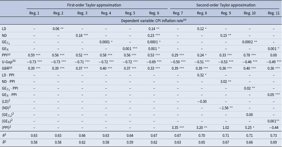
We put the first-order terms of equation (31) into a panel data regression model in which we explain the CPI inflation rate by the spillover effects $\varsigma _{\mathcal {A}}$ and the shocks $\boldsymbol{u}$ . We proxy the spillover effects by the network topology ( $\textrm {NT} (\tilde {\mathcal {A}}_{})$ ) measures (link density, network density and graph energy) as motivated in Section 2.4. For the shock elements $\boldsymbol{u}$ , we use the variables of a classical Phillips curve specification, namely: the producer price index (PPI), the cyclical unemployment gap (U-Gap)Footnote ²⁴ and in addition to this, a long-term interest rate (10-year government bond rate, GBR) (see and the references there in Aguiar and Martins Reference Aguiar and Martins2005; Hazell et al. Reference Hazell, Herreño, Nakamura and Steinsson2022). We create an appropriate time variation of the network (compare Holme and Saramäki Reference Holme and Saramäki2012) by estimating equation (15) over different time windows of 60 months each, with an overlap to obtain estimates for a total of nine windows.Footnote ²⁵ We use the adjacency matrix $\tilde {\mathcal {A}}_{c,t}$ of each window $t=1,\ldots, 9$ to compute the network topology measuresFootnote ²⁶ and we do this for each country $c=1,\ldots, 28$ . Importantly, we use the median across the draws of the posterior distribution of $\tilde {\mathcal {A}}_{c,t}$ for each country and time-window. Figure 6 illustrates the variation in the four network topology measures and the CPI inflation rate (median and 68-percentile across countries) over time and across countries. The width of the boxes indicates the variation across countries. The median estimate demonstrates the variation over time.

We estimate a panel data regression model of the form

(32) \begin{equation} \pi _{c,t}=\beta _{\textrm {NT}} \cdot \textrm {NT}\left (\tilde {\mathcal {A}}_{c,t}\right ) + \sum _{i\geq 1}^K\beta _i x_{c,t,i} + e_{c,t} \end{equation}

to explain the CPI inflation rate $\pi _{c,t}$ . As regards equation (32), the $K=3$ explanatory variables ( ${x}_{c,t,i})$ next to the network topology measure $\textrm {NT}\left (\tilde {\mathcal {A}}_{c,t}\right )$ are given by the PPI, the unemployment gap (U-Gap) and the GBR, $e_{c,t}$ is the error term, $c$ denotes the country and $t$ the time variation. The temporal variation $t$ is limited to the nine time windows. All variables are based on a monthly frequency. The price variables (CPI, PPI) are expressed as relative changes (year-over-year changes). The value of all variables within the nine windows is calculated as the mean value of the corresponding months.

We use the fixed effects (FEs) estimator as it is considered to be the adequate approach for a situation where there are unobservable country effects and unobservable time effects. The results are provided in Table 2, where we report the estimates of distinct specifications of equation (32) (Reg. 1 to Reg. 6). The first regression (Reg. 1) does not include any of the network topology measures and the estimates for the partial effects of the remaining explanatory variables (PPI, U-Gap, GBR) are in each case statistically significantly different from zero at least at the one percent level and all parameter estimates have their expected signs. For example, the estimates indicate, that a one percentage point increase in the producer price inflation rate leads to an increase in the CPI inflation rate of 0.6 percentage points; this partial effect turns out higher in the case of the unemployment gap (−0.73). Finally, while the positive estimate for the GBR aligns with the Fisher-effect, the estimated value, however, clearly subceeds unity as would be expected from theory (see Wickens, Reference Wickens2012 Chapter 14.2).

Table 2.

Network topology measures and the consumer price index (CPI) inflation rate

Notes: The table reports the results from a panel data fixed effects regression model. The acronyms refer to link density (LD), network density (ND) and graph energy (GE) for the network topology measures and producer price index (PPI), unemployment gap (U-Gap) and 10-year government bond rate (GBR) for the remaining explanatory variables. For each regression, the number of observations is $N\cdot T=252$ with $T=9$ and $N=28$ . The asterisks refer to the following levels of statistical significance: $^{***}$ for 1 percent, $^{**}$ for 5 percent and $^{*}$ for 10 percent. $\bar {R}^2$ refers to the adjusted $R^2$ . The inflation rates of the CPI, PPI, the unemployment gap and the government bond rate are calculated as monthly averages for each of the nine windows. The unemployment gap (U-Gap) is measured by the cyclical component of the year-over-year change in unemployment, extracted using the Hodrick-Prescott filter with a smoothing parameter of 14,400.

In a sequential extension of the basic regression model (Reg. 1) to include the network topology measures, we find that, first, link density (Reg. 2) is statistically significant in explaining the CPI inflation rate. This confirms the importance of cross-price dependencies for the CPI inflation rate in general. The point estimate implies that an increase in the number of links by one percent raises the inflation by 0.06 percentage points. While this concerns only the diffusion effect, we also find evidence in favor of the strength effect: the network density (Reg. 3) has a high statistical support for explaining the variation in the CPI inflation rate. Its point estimate implies that an increase in the network density by one percent raises the inflation rate by 0.18 percentage points. While link density has indicated the significant role of the diffusion effect, network density implies that the strength effect is of even higher importance. This can be seen by both the significantly higher partial effect, and by the increase in the goodness-of-fit measures (normal $R^2$ and adjusted $R^2$ , the latter being denoted as $\bar {R}^2$ ) of Reg. 3 relative to Reg. 2.

Finally, the graph energy (Reg. 4 and Reg. 5) has a high explanatory power for the CPI inflation rate. This is the case for both measures (GE $_{\mathbb {Z}_2}$ and GE $_{\mathbb {R}}$ ). Although the coefficient estimate of the binary graph energy measure (GE $_{\mathbb {Z}_2}$ ) is small, this should not obscure the importance of this variable, especially as its values are high (see Figure 6). The fact that the graph energy measures have a statistically significant impact on the inflation rate highlights the role of cyclical interdependencies between the price sub-indices (see Figure 1). Cyclical interdependencies imply that the effects of microeconomic price shocks are slow to dissipate, resulting in long-lasting effects of microeconomic price shocks on the CPI inflation rate, hence shaping its inertia.

The simultaneous utilization of all four network topology measures in the regression model (Reg. 6) yields statistically significant results at least at the 10% level. This corroborates the important role of both the diffusion and strength effects.

4.2 Second-order terms

We now extend the panel data regression model given by equation (32) to include the second-order terms of equation (31). We estimate the extended model again using the FEs estimator and provide the results in the last five columns (Reg. 7 to Reg. 11) of Table 2. We present results involving the interaction terms only between the PPI and the four network topology measures; this is because in all other cases (this includes also the second-order terms of the unemployment gap and the GBR) the results are not statistically significant.

The results highlight that in all cases (Reg. 7 to 11) the unemployment gap (U-Gap) and the GBR keep their high level of statistical significance. As regards the PPI, both the first-order terms and the quadratic terms are statistically significant (consider Reg. 7) and the partial effect is given by $\frac {\partial \pi }{\partial \textrm {PPI} } = 0.45$ (the mean value of the PPI was used: $\overline {\textrm {PPI}}=0.03$ ), which subceeds that of the first-order terms model.

When the network topology measures (Reg. 8 to Reg. 11) are added, the quadratic term of the PPI loses its high level of statistical significance in some cases. The partial effect of the PPI $\partial \pi / \partial \textrm {PPI}$ is now given by 0.43 for Reg. 8, 0.42 for Reg. 9, 0.47 for Reg. 10 and 0.44 for Reg. 11, when using the mean values for the relative change in the PPI ( $\overline {\textrm {PPI}}=0.03$ ), the link density ( $\overline {\textrm {LD}}=0.12$ ), the network density ( $\overline {\textrm {ND}}=0.01$ ) and the graph energy measures ( $\overline { \textrm {GE}}_{ \mathbb {Z}_2} = 32.2$ and $\overline { \textrm {GE}}_{ \mathbb {R}} = 9.8$ ).

We find the following partial effects of the network topology measures on the CPI inflation (noting the interaction and second-order terms): $\frac {\partial \pi }{\partial \textrm {LD} } = 0.05$ , $\frac {\partial \pi }{\partial \textrm {ND} } = 0.18$ , $\frac {\partial \pi }{\partial \textrm {GE}_{\mathbb {Z}_2} } = 0.0001$ , and $\frac {\partial \pi }{\partial \textrm {GE}_{\mathbb {R}} } = 0.001$ . They all align well in size with the corresponding estimates of the first-order regressions (Reg. 2 to Reg. 5).

Most importantly, however, we find that the terms for $f_{\varsigma _{\mathcal {A}} u }$ in equation (31), given by $\frac {\partial ^2\pi }{\partial \textrm {PPI} \cdot \partial \textit {LD}} = 0.32$ , $\frac {\partial ^2\pi }{\partial \textrm {PPI} \cdot \partial \textit {ND}} = 3.02$ , $\frac {\partial ^2\pi }{\partial \textrm {PPI} \cdot \partial \textit {GE}_{\mathbb {Z}_2}} \approx 0.02$ and $\frac {\partial ^2\pi }{\partial \textrm {PPI} \cdot \partial \textit {GE}_{\mathbb {R}}} = 0.05$ from the panel data regression results are all positive. Moreover, these parameter values are all statistically different from zero. This implies that the transmission mechanism of changes in the producer prices to the CPI inflation rate are shaped by the demand-driven cross-price dependencies. More specifically, the demand-driven cross-price dependencies exacerbate any change in the producer prices on the CPI inflation rate. With a view to the link density and the binary graph energy, the extent of shock exacerbation occurs due to the diffusion effect. As the results of the network density and the non-binary graph energy highlight, the strength effect is also important alongside to the diffusion effect. Most importantly, the strength effect exacerbates the diffusion effect—this can again be seen by the increase in the goodness-of-fit measures (normal $R^2$ and adjusted $R^2$ ) of Reg. 9 and 11 relative to Reg. 8 and 10.

4.3 Further remarks

The results presented here are robust to various extensions in the form of additional variables used in the VAR model, alternative approaches to identifying the VAR models, additional explanatory variables in the panel data regression model, and the use of robust standard errors. In addition, we examined the sensitivity of the panel data regression to the time span of the Covid-19 pandemic, the subsequent global recovery and significant geopolitical turmoil (military invasions of Iraq, Lebanon, Libya, Ukraine, etc.). Our baseline results remain qualitatively robust to these changes and extensions. Additional robustness checks are discussed in the Online Appendix.

It is important to note that our regression analysis may suffer from the “generated regressor” problem, which occurs when the regressors themselves are estimated rather than directly observed. This can lead to biased standard errors and thus invalid inference. To mitigate this problem, an alternative approach would be to estimate the first- and second-order regression equations repeatedly over all draws from the posterior distribution of the network topology measures. This method would ensure that the variability and uncertainty in the network measures are adequately captured, resulting in more robust and reliable estimates.

Finally, we attempted to estimate the (32) equation using the network topology measures based on the supply-driven cross-price dependencies ( $\tilde {\Gamma }$ ). However, significant data limitations hamper the implementation. On the one hand, calibration is not possible for some countries because I-O tables are not available. On the other hand, for many other countries, I-O tables are only available for a limited number of recent years. This limits both the time span and the country coverage, rendering impossible a proper estimation of equation (32).