1 Introduction
Mass loss from the Antarctic and Greenland Ice Sheets represents an important contribution to global sea level rise. This mass loss is predominantly occurring where ice sheets meet the polar oceans, and is strongly affected by ocean properties. The response of these ice sheets to a warmer climate is uncertain, making predictions of future sea level rise difficult. As such, a greater understanding of the processes occurring at the ice–ocean interface is needed to constrain possibilities of the future climate.
The mass loss from the Antarctic and Greenland Ice Sheets can be due to either melting or dissolving, depending on the temperature and salinity of the ocean. If the ambient fluid is sufficiently warm (or fresh), ice will melt (Woods Reference Woods1992; Kerr Reference Kerr1994b
). Melting is controlled solely by heat transfer and will result in the interface salinity being zero and the interface temperature being the pressure-dependent melting point. In contrast, when the ambient fluid is sufficiently cold (or salty), ice will dissolve (Kerr Reference Kerr1994a
). Dissolving is controlled both by heat and salt transfer, and will result in the interface salinity being non-zero and the interface temperature being below the pressure-dependent melting point. At oceanic salinities, ice will dissolve in temperatures less than approximately
 $6\,^{\circ }\text{C}$
(Kerr & McConnochie Reference Kerr and McConnochie2015). As such, the relevant regime in an oceanic environment is the dissolution of ice, rather than the melting.
Laboratory experiments and theoretical analysis have been conducted that investigate the ablation velocity, interface temperature (Kerr & McConnochie Reference Kerr and McConnochie2015) and plume properties (McConnochie & Kerr Reference McConnochie and Kerr2016b
) when ice dissolves into homogeneous salty water. It was found that the ablation rate and interface temperature are uniform with height, and that the plume velocity increases like
 $z^{1/3}$
. Direct numerical simulations have recently been used to investigate the same problem of ice dissolving into homogeneous salty water, and they strongly agree with the experimental results (Gayen, Griffiths & Kerr Reference Gayen, Griffiths and Kerr2016). The effect of an ambient salinity gradient on the ice and plume properties has also been investigated (McConnochie & Kerr Reference McConnochie and Kerr2016a
). An ambient salinity gradient is seen to reduce the ablation velocity, interface temperature, plume velocity and plume acceleration. Stratification also causes the ablation velocity to reduce with height.
Observations next to Greenland glaciers during the summer months have shown that subglacial plumes are frequently released at the grounding line of these glaciers (Straneo & Cenedese Reference Straneo and Cenedese2015). During the summer, ice melts on the inland surface of the ice sheets. The meltwater then flows down to the bedrock and under the outlet glaciers before being released into the ocean at the grounding line, where it rises as buoyant plumes at various locations along the ice face (Fried et al. Reference Fried, Catania, Bartholomaus, Duncan, Davis, Stearns, Nash, Shroyer and Sutherland2015). Subglacial plumes are almost always associated with high ablation rates (Fried et al. Reference Fried, Catania, Bartholomaus, Duncan, Davis, Stearns, Nash, Shroyer and Sutherland2015). As such, the stability of the Greenland Ice Sheet is likely to be highly dependent on the strength of these subglacial plumes and how they affect the ice–ocean interface.
Direct observation of the ice–ocean interface is extremely challenging due to the isolated location of tidewater glaciers. Processes occurring at the ice face are typically inferred from observations made some distance downstream of the ice face (e.g. Beaird, Straneo & Jenkins Reference Beaird, Straneo and Jenkins2015). The plumes are typically assumed to have zero salinity and be at the pressure-dependent freezing point. In one particular fjord, the volume flux of the subglacial plume discharged at the base of two typical Greenland glaciers was estimated to be roughly four times the meltwater volume flux in the region of the plume (Beaird et al. Reference Beaird, Straneo and Jenkins2015). This estimation was made using multiple noble gases as water type tracers, increasing the reliability of the result compared to other studies that typically use only temperature and salinity to estimate water type fractions.
Laboratory experiments have previously been conducted that examine the effect of a subglacial plume on a vertical ice face (Cenedese & Gatto Reference Cenedese and Gatto2016). This study was focused on the effect of two interacting plumes released into a two-layer stratification. The plumes were initially separated, but merged at some location up the ice wall. The conditions where the plume reaches the surface and where it intrudes at mid-depth were explored, as well as the spatially averaged ablation rate of the ice.
A number of numerical modelling studies have also investigated the effect of these subglacial plumes on ice–ocean interactions (e.g. Xu et al. Reference Xu, Rignot, Menemenlis and Koppes2012, Reference Xu, Rignot, Fenty and Menemenlis2013; Carroll et al. Reference Carroll, Sutherland, Shroyer, Nash, Catania and Stearns2015). The majority of recent numerical studies have used a parameterization of ice–ocean processes that uses constant thermal and compositional Stanton numbers to describe the transport of heat and salt (Jenkins Reference Jenkins2011). This parameterization will hereafter be referred to as the three-equation model. The three-equation model was originally developed based on heat transfer in turbulent boundary layers (Jenkins Reference Jenkins1991) and has since been adjusted to reflect different turbulent transfer relationships and thermodynamic balances (e.g. Lane-Serff Reference Lane-Serff1995; Holland & Jenkins Reference Holland and Jenkins1999; Jenkins Reference Jenkins2011). Despite being extensively used in numerical investigations, it has not been properly validated against field observations due to the difficulty in accurately making measurements close to the ice–ocean interface.
Straneo & Cenedese (Reference Straneo and Cenedese2015) summarize the results of recent numerical modelling studies by suggesting that ‘the submarine melt rate increases with increasing subglacial discharge (with a power of
 $1/3$
), linearly increases with increasing temperature, and increases with vertical distance above the grounding line in winter and slightly decreases with it in summer.’
This paper presents experiments that investigate the effect of a turbulent two-dimensional subglacial plume on the ice ablation rate and interface temperature. In particular, we examine the behaviour of the wall plume as it transitions from being dominated by the distributed buoyancy flux due to dissolution, to being dominated by the external source of buoyancy at the base of the ice. These experiments use a much larger tank than those performed by Cenedese & Gatto (Reference Cenedese and Gatto2016), enabling the observation of the plume velocity, the ablation velocity and the interface temperature as a function of height.
In § 2 we present models of the turbulent plume that forms due to a vertically distributed source of buoyancy and due to a line source of buoyancy next to a wall. The experimental method and techniques are then described in § 3. The experimental results are presented in § 4. Finally, we examine oceanographic data from a variety of tidewater glaciers and compare them to our experimental results in § 5.
2 Theoretical scaling
Our experiments lie between two limiting cases. These can be described by a non-dimensional parameter,
 $B^{\ast }$
, defined as:
 $$\begin{eqnarray}B^{\ast }=\frac{B_{s}+B_{o}}{B_{o}},\end{eqnarray}$$
where
 $B_{s}$
is the imposed buoyancy flux from the freshwater source and
 $B_{o}$
is the buoyancy flux that would be expected due to ablation of the ice wall without an external plume (Kerr & McConnochie Reference Kerr and McConnochie2015). The theory presented in Kerr & McConnochie (Reference Kerr and McConnochie2015) is based on heat transfer relationships through the turbulent plume that forms next to a heated plate. The model has been extended to the case of a dissolving ice wall, and is seen to accurately predict the ablation rate and interface conditions based on the ambient fluid temperature and salinity. A buoyancy flux based on the predicted ablation rate and interface conditions is then calculated as
 $$\begin{eqnarray}B_{o}=VgHW\left(\frac{\unicode[STIX]{x1D70C}_{s}}{\unicode[STIX]{x1D70C}_{i}}\right)\left(\frac{\unicode[STIX]{x1D70C}_{f}-\unicode[STIX]{x1D70C}_{i}}{\unicode[STIX]{x1D70C}_{f}}\right)(1-{\mathcal{R}}^{-1}),\end{eqnarray}$$
where
 $V$
is the predicted ablation velocity,
 $g$
is the acceleration due to gravity,
 $H$
and
 $W$
are the height and the width of the ice wall,
 $\unicode[STIX]{x1D70C}_{s}$
,
 $\unicode[STIX]{x1D70C}_{i}$
and
 $\unicode[STIX]{x1D70C}_{f}$
are the densities of the ice, the interface fluid and the ambient fluid, respectively, and
 ${\mathcal{R}}$
is the ratio of the compositional to thermal buoyancy (Kerr & McConnochie Reference Kerr and McConnochie2015).
Both the experiments and theory presented in Kerr & McConnochie (Reference Kerr and McConnochie2015) suggest that the ablation rate is constant with height. As such, it is assumed that
 $B_{o}$
, the buoyancy flux due to ablation of the ice, is constant with height. Numerical simulations suggest that the ablation rate decreases slightly with height when the subglacial buoyancy flux is important and increases with height when it is not (Straneo & Cenedese Reference Straneo and Cenedese2015). The assumption of a constant ablation rate is therefore unlikely to be true on geophysical scales, but represents a reasonable approximation.
When
 $B_{s}=0$
, there is no imposed buoyancy flux and
 $B^{\ast }=1$
. This represents the wall plume from a distributed source described by McConnochie & Kerr (Reference McConnochie and Kerr2016b
). Alternatively, when
 $B_{s}\gg B_{o}$
,
 $B^{\ast }$
will be large and the distributed buoyancy flux from the wall will be negligible. Here the plume can be described as a wall plume from a line source of buoyancy at the base of the wall.
A limitation of the definition of
 $B^{\ast }$
given in (2.1) is that it varies with position up the ice wall. At very low heights, the buoyancy flux from the wall will always be negligible, while at sufficiently large heights the source buoyancy flux will become negligible. The definition given in (2.1) is useful for considering changes in behaviour in our fixed height domain, but less useful when considering the behaviour of the plume at a given height. To consider the behaviour of the plume at various locations, a height-dependent definition of
 $B^{\ast }$
could be used:
 $$\begin{eqnarray}B_{z}^{\ast }=\frac{B_{s}/\unicode[STIX]{x1D6F7}+z}{z}=\frac{H(B^{\ast }-1)+z}{z},\end{eqnarray}$$
where
 $\unicode[STIX]{x1D6F7}$
is the buoyancy flux per unit height,
 $z$
is the vertical location up the wall and
 $H$
is the total height of the domain used in (2.1).
2.1 The wall plume from a distributed source of buoyancy
McConnochie & Kerr (Reference McConnochie and Kerr2016b ) conducted experiments examining the turbulent wall plume that forms next to a dissolving vertical ice face. The distributed flux of buoyancy and the presence of a wall both impacted the plume properties. In particular, the presence of a wall was seen to impose a significant drag on the plume, resulting in a reduced velocity. The entrainment coefficient based on a characteristic top-hat velocity was observed to be 0.048. The following top-hat model for a distributed wall plume was obtained:
 $$\begin{eqnarray}\displaystyle & b_{T}=0.036z, & \displaystyle\end{eqnarray}$$
 $$\begin{eqnarray}\displaystyle & w_{T}=1.2\unicode[STIX]{x1D6F7}^{1/3}z^{1/3}, & \displaystyle\end{eqnarray}$$
 $$\begin{eqnarray}\displaystyle & \unicode[STIX]{x1D6E5}_{T}=23\unicode[STIX]{x1D6F7}^{2/3}z^{-1/3}, & \displaystyle\end{eqnarray}$$
 $$\begin{eqnarray}\displaystyle & Q=0.043\unicode[STIX]{x1D6F7}^{1/3}z^{4/3}, & \displaystyle\end{eqnarray}$$
where
 $b_{T}$
is the top-hat plume width,
 $w_{T}$
is the top-hat plume velocity,
 $\unicode[STIX]{x1D6E5}_{T}$
is the top-hat plume buoyancy,
 $Q$
is the plume volume flux,
 $z$
is the height above a virtual source and
 $\unicode[STIX]{x1D6F7}$
is the buoyancy flux per unit area. Equations (2.4)–(2.7) imply a large frictional stress acting on the plume. Gayen et al. (Reference Gayen, Griffiths and Kerr2016) calculate this frictional stress,
 $\unicode[STIX]{x1D716}$
, to be equal to 65 % of the upwards buoyancy force, and describe it using a drag coefficient,
 $c_{D}=\unicode[STIX]{x1D716}/w_{M}^{2}=0.06$
, where
 $w_{M}$
is the maximum plume velocity.
2.2 The two-dimensional line plume
The two-dimensional line plume has been extensively studied in the past (see Fischer et al.
Reference Fischer, List, Koh, Imberger and Brooks1979). The properties of a line plume can be described by the source buoyancy flux,
 $B_{s}$
, and the height above a virtual source,
 $z$
. The maximum plume velocity,
 $w_{M}$
, and the plume volume flux,
 $Q$
, are:
 $$\begin{eqnarray}\displaystyle & w_{M}=1.66B_{s}^{1/3}, & \displaystyle\end{eqnarray}$$
 $$\begin{eqnarray}\displaystyle & Q=0.34B_{s}^{1/3}z. & \displaystyle\end{eqnarray}$$
Measurements of the entrainment coefficient have been made with a vertical wall, a sloping wall or without a wall. Ellison & Turner (Reference Ellison and Turner1959) showed that the entrainment coefficient reduces as the overall Richardson number (a measure of the stability of a plume or gravity current) increases or the slope becomes shallower. For the case of a plume next to a vertical wall, an entrainment coefficient based on the average plume velocity of 0.087 was measured. This compares to a two-dimensional line plume without a wall, where a significantly higher entrainment coefficient of 0.22 was described.
Grella & Faeth (Reference Grella and Faeth1975) conducted experiments on a line plume next to a vertical wall, and measured across plume velocity and density profiles. They reported an entrainment coefficient based on the average plume velocity of
 $0.095\pm 0.005$
, which corresponds to an entrainment coefficient of
 $0.067\pm 0.004$
based on the maximum velocity. Similar measurements of entrainment into a line plume next to a vertical wall were made by Sangras, Dai & Faeth (Reference Sangras, Dai and Faeth1999), who observed a lower entrainment coefficient of 0.076. The measurements of the characteristic plume width made by Sangras et al. (Reference Sangras, Dai and Faeth1999) were made at heights greater than 100 source diameters to ensure that the wall plume was in a self-preserving flow regime. Previous measurements were made at lower heights where the wall plume may still have been transitioning to a self-preserving regime.
The decrease in entrainment coefficient due to the presence of a wall is consistent across all experiments, and has been explained by the wall limiting the swaying motion that line plumes often display (Turner Reference Turner1973) and inhibiting the large-scale, cross-stream turbulent motion that is required for effective mixing (Grella & Faeth Reference Grella and Faeth1975; Sangras et al. Reference Sangras, Dai and Faeth1999).
2.3 The wall plume from a line source of buoyancy
We now reformulate (2.8) and (2.9) to include a generalized entrainment coefficient,
 $\unicode[STIX]{x1D6FC}$
, and drag coefficient,
 $c_{D}$
. Conservation of buoyancy flux, volume flux and momentum flux gives:
 $$\begin{eqnarray}\displaystyle & B_{s}=b_{T}w_{T}\unicode[STIX]{x1D6E5}_{T}, & \displaystyle\end{eqnarray}$$
 $$\begin{eqnarray}\displaystyle & \displaystyle \frac{\text{d}Q}{\text{d}z}=\frac{\text{d}(b_{T}w_{T})}{\text{d}z}=\unicode[STIX]{x1D6FC}w_{T}, & \displaystyle\end{eqnarray}$$
 $$\begin{eqnarray}\displaystyle & \displaystyle \frac{\text{d}M}{\text{d}z}=\frac{\text{d}(b_{T}w_{T}^{2})}{\text{d}z}=b_{T}\unicode[STIX]{x1D6E5}_{T}-c_{D}w_{T}^{2}, & \displaystyle\end{eqnarray}$$
where
 $M$
is the plume momentum flux and
 $\unicode[STIX]{x1D6E5}_{T}$
is the top-hat plume buoyancy.
Based on (2.8) and (2.9) we assume functional forms for
 $b_{T}$
and
 $w_{T}$
of:
 $$\begin{eqnarray}b_{T}=c_{1}z\quad \text{and}\quad w_{T}=c_{2}B_{s}^{1/3},\end{eqnarray}$$
where
 $c_{1}$
and
 $c_{2}$
are unknown constants. This leads to an expression for
 $\unicode[STIX]{x1D6E5}_{T}$
from (2.10) of:
 $$\begin{eqnarray}\unicode[STIX]{x1D6E5}_{T}=\frac{B_{s}^{2/3}}{c_{1}c_{2}z}.\end{eqnarray}$$
 $$\begin{eqnarray}\displaystyle & b_{T}=\unicode[STIX]{x1D6FC}z, & \displaystyle\end{eqnarray}$$
 $$\begin{eqnarray}\displaystyle & \displaystyle w_{T}=\left(\frac{B_{s}}{\unicode[STIX]{x1D6FC}+c_{D}}\right)^{1/3}, & \displaystyle\end{eqnarray}$$
 $$\begin{eqnarray}\displaystyle & \displaystyle \unicode[STIX]{x1D6E5}_{T}=\frac{B_{s}^{2/3}(\unicode[STIX]{x1D6FC}+c_{D})^{1/3}}{\unicode[STIX]{x1D6FC}z}. & \displaystyle\end{eqnarray}$$
Equations (2.15) and (2.16) can be used to find expressions for the plume volume and momentum flux:
 $$\begin{eqnarray}\displaystyle & \displaystyle Q=b_{T}w_{T}=\frac{\unicode[STIX]{x1D6FC}B_{s}^{1/3}z}{(\unicode[STIX]{x1D6FC}+c_{D})^{1/3}}, & \displaystyle\end{eqnarray}$$
 $$\begin{eqnarray}\displaystyle & \displaystyle M=b_{T}w_{T}^{2}=\frac{\unicode[STIX]{x1D6FC}B_{s}^{2/3}z}{(\unicode[STIX]{x1D6FC}+c_{D})^{2/3}}. & \displaystyle\end{eqnarray}$$
Wells & Worster (Reference Wells and Worster2008) developed a theoretical model for natural convection next to an isothermal surface. They described two regimes based on whether the inner sublayer is driven by its own buoyancy or by the shear imposed upon it. Within the shear-driven regime a drag coefficient of 0.0046 was calculated (Wells & Worster Reference Wells and Worster2008). Jenkins (Reference Jenkins1991, Reference Jenkins2011) estimated the drag coefficient to be 0.0025 next to tidewater glaciers. Both of these estimates are an order of magnitude smaller than the previously described estimates of the entrainment coefficient for turbulent wall plumes, which allows
 $c_{D}$
to be neglected in (2.16)–(2.19).
3 Experiments
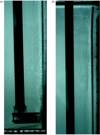
Experiments have been conducted to examine the effect of a cold freshwater line plume next to a vertical ice face. The experiments were carried out in a tank that was 1.2 m high, 1.5 m long and 0.2 m wide, with an overflow 1.1 m from the base. Figure 1 shows a photo from an experiment with
 $B^{\ast }=21.2$
that has been visualized using the shadowgraph technique. Ice can be seen on the right of the tank and the quiescent ambient fluid on the left. The external plume was seen to attach to the ice face as it is released. For experiments performed at lower values of
 $B^{\ast }$
the transition to turbulence was sometimes further up the ice wall, but never as much as 10 cm from the source location.
A shadowgraph image of an experiment with
 $B^{\ast }=21.2$
. The ice can be seen on the right hand side of the tank and the quiescent ambient fluid on the left. Immediately next to the ice the turbulent wall plume can be seen. (a) Image for the base of the tank up to a height of 59 cm. (b) Image from a height of 49 cm to the free surface at 110 cm.

The tank was kept in a temperature-controlled room at approximately
 $4\,^{\circ }\text{C}$
. Approximately 5–10 cm of ice was grown from fresh water before being exposed to a NaCl solution with a concentration,
 $C_{f}$
, of approximately 3.5 wt % NaCl. After the far-field salinity and temperature were measured with a conductivity–temperature probe, the line plume was initiated.
The volume flux of the line plume was controlled with a peristaltic pump and kept constant throughout an experiment. The volume flux was measured at the end of an experiment by measuring the time taken to fill a volumetric flask from the outflow. The fluid for the line plume was cooled to approximately
 $0\,^{\circ }\text{C}$
before the experiment was commenced, then kept at this temperature throughout an experiment. The temperature of the line plume fluid was measured both in the reservoir and as it was released at the base of the tank.
Due to heat transfer through the peristaltic pump and through the piping between the reservoir and the source, the temperature of the plume fluid was generally between 0.1 and
 $1.1\,^{\circ }\text{C}$
when it was released. For three experiments with a very small source volume flux (
 $Q_{s}<1.5~\text{ml}~\text{s}^{-1}$
) we were unable to keep the source temperature below
 $1.1\,^{\circ }\text{C}$
, as the fluid spent a long time flowing between the storage reservoir and the outflow. However, the plume was observed to rapidly entrain ambient fluid, so the effect of this should be minimal apart from very close to the source. This is supported by (2.17), which shows the plume buoyancy decreasing like
 $1/z$
. We would therefore expect the plume temperature to quickly tend towards the ambient fluid temperature, minimizing the impact of the warmer source temperatures at low values of
 $B^{\ast }$
. The height required for the source plume buoyancy to reduce by 90 % is 5.4 cm for the experiment at
 $B^{\ast }=33.1$
, and less for lower values of
 $B^{\ast }$
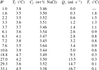
. Since all measurements were made above this height we do not expect the plume source conditions to significantly affect the experimental results. Table 1 shows the experimental parameters and the computed values of
 $B^{\ast }$
.
Experimental parameters for all experiments. All results are reported in terms of the non-dimensionalized buoyancy flux,
 $B^{\ast }$
.
 $T_{f}$
and
 $C_{f}$
are the far-field fluid temperature and salinity respectively.
 $Q_{s}$
is the source volume flux and
 $T_{s}$
is the source temperature.
 $T_{s}$
is measured inside the expansion chamber and is approximately 5 cm from the source outflow.

Immediately before being released, the line plume fluid passed through a chamber to ensure that it was released uniformly across the width of the tank. This chamber consisted of a thin slot the full width of the tank. The upper edge of the chamber was 6 cm above the base of the tank. The source fluid was visualized with dye to confirm that it was released evenly over the full width of the tank. The end of the chamber was placed flush against the ice at the start of an experiment. Throughout an experiment, the ice retreated away from the chamber, leaving a gap of up to 3 cm between the chamber and the ice. Despite this gap the plume quickly became attached to the ice face, due to the Coandă effect (Wille & Fernholz Reference Wille and Fernholz1965), and there was no measurable change in the across plume velocity profile as a result of this short separation.
Throughout an experiment the ablation velocity and interface temperature were measured as described in Kerr & McConnochie (Reference Kerr and McConnochie2015). Thermistors were frozen into the ice at heights of 43, 50, 55 and 68 cm above the base of the tank. A second thermistor was positioned 68 cm above the base of the tank to confirm that there was no horizontal variation in interface temperature. Since the ablation rates in these experiments were larger than those in Kerr & McConnochie (Reference Kerr and McConnochie2015), the time period over which the ablation velocity was measured was reduced. For the highest flow rates the ablation velocity was measured over intervals of 5 min. For lower flow rates this time interval was progressively increased up to 15 min. Measurements of the ablation velocity were made at least four times, then averaged to reduce the uncertainty in measurements and to confirm that the ablation velocity was constant.
The plume velocity was measured using the Particle Tracking Velocimetry (PTV) technique. Pliolite particles of diameter
 $125{-}250~\unicode[STIX]{x03BC}\text{m}$
were seeded into the ambient fluid and were then entrained into the line plume. The particle density was measured by settling into a salinity gradient. The measured density of approximately
 $1025~\text{kg}~\text{m}^{-3}$
gives a calculated rise velocity of
 $0.03$
–
 $0.12~\text{mm}~\text{s}^{-1}$
in the ambient fluid, depending on the particle size. This particle rise velocity is negligible compared to typical plume velocities, which vary from
 $14~\text{mm}~\text{s}^{-1}$
at the lowest source flow rates to
 $37~\text{mm}~\text{s}^{-1}$
at the highest source flow rate. The PTV software ‘Streams’ (Nokes Reference Nokes2014) was used for particle identification, particle tracking and the computation of velocity fields.
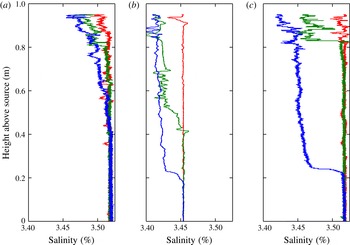
The first front position and far-field properties were measured as in McConnochie & Kerr (Reference McConnochie and Kerr2016b
) with a traversing conductivity–temperature probe. Some example profiles are shown in figure 2. The first front is seen to propagate more rapidly for experiments performed at higher values of
 $B^{\ast }$
. The shape of the first front also changes. At high values of
 $B^{\ast }$
, there is a large step change in salinity at the first front and a weak gradient above it. However, as observed by McConnochie & Kerr (Reference McConnochie and Kerr2016b
) in the absence of a source plume, lower values of
 $B^{\ast }$
do not have a step change in salinity at the first front. The behaviour at low values of
 $B^{\ast }$
is consistent with the peeling detrainment mechanism (Hogg Reference Hogg2014; Hogg et al.
Reference Hogg, Dalziel, Huppert and Imberger2016), while the step change in buoyancy at high values of
 $B^{\ast }$
is typical of standard models of the turbulent filling box (Baines & Turner Reference Baines and Turner1969; Worster & Huppert Reference Worster and Huppert1983).
Salinity profiles for three different experiments. (a)
 $B^{\ast }=2.2$
, with the profiles made 10 min apart from one another. (b)
 $B^{\ast }=7.2$
and (c)
 $B^{\ast }=29.3$
, with the profiles made 5 min apart from one another. The first front is seen to propagate down the tank throughout an experiment. The first profile (red) was made before the source plume was initiated, and shows the initial salinity profile.

4 Experimental results
4.1 Plume velocity
For our experiments performed at sufficiently low source flow rates we would expect the external buoyancy flux to be unimportant. This will lead to a turbulent wall plume that can be described by the model for a vertically distributed source of buoyancy, and hence (2.4)–(2.7). However, as the source flow rate is increased, its buoyancy flux will become much larger than the buoyancy flux due to ablation of the ice wall. At a sufficiently high source flow rate, the plume properties will be dominated by the freshwater source at the base of the wall, and the buoyancy flux due to ablation of the ice can be neglected. In this regime, the scaling described in (2.15)–(2.19) will accurately describe the turbulent wall plume.
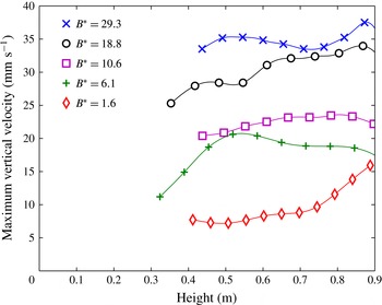
Measured maximum vertical velocities as a function of height for five typical experiments. The height is measured from the release point of the source plume (6 cm above the bottom of the tank).

Figure 3 shows the measured vertical velocity with height for five different experiments. The plume velocity was measured continuously up the ice wall, and the markers shown on figure 3 are only to differentiate between values of
 $B^{\ast }$
. The experimental data have been smoothed using a smoothing spline to remove the effect of erroneous measurements. The raw data had a typical scatter of
 $\pm 2.5~\text{mm}~\text{s}^{-1}$
. The experiments cover a range of
 $B^{\ast }$
of 1.6–29.3 and heights from approximately 30 to 90 cm. Heights below 30 cm could not be measured due to several experimental limitations. Most significantly, it was difficult to seed particles at the base of the plume without imposing an additional vertical velocity. At higher locations entrainment could be used to seed the plume with particles, but at low heights the particles needed to be added directly to the plume. Additionally, density gradients were larger at the base of the plume, leading to larger uncertainties due to light refraction. Above 90 cm, the velocity reduces as an overturning eddy from the free surface becomes important.
The experiment conducted at the lowest source flow rate (
 $B^{\ast }=1.6$
) shows a velocity of a similar magnitude to that from a distributed source of buoyancy (McConnochie & Kerr Reference McConnochie and Kerr2016b
). Consistent with results from a distributed source of buoyancy, the plume continues to accelerate up the ice wall, although the rate of acceleration appears to be higher in these experiments. For flow rates above this, the plume behaves more like that from a line source of buoyancy. In this regime there is an initial acceleration region before the plume reaches a constant velocity. The initial acceleration region can be seen in the data for
 $B^{\ast }=6.1$
, but is below the measurement region for the other three experiments.
Measured maximum vertical velocity as a function of
 $B^{\ast }$
. The solid line shows the predicted vertical velocity based on the model of a wall plume from a line source of buoyancy described in § 2. It is assumed that the drag coefficient is negligible and an entrainment coefficient of 0.075 is used based on the experimental data. The dashed line shows the maximum vertical velocity from McConnochie & Kerr (Reference McConnochie and Kerr2016b
) for a buoyancy flux per unit area of
 $4.5\times 10^{-7}~\text{m}^{2}~\text{s}^{-3}$
and a height of 80 cm. This value of
 $\unicode[STIX]{x1D6F7}$
corresponds to a far-field temperature of
 $4.1\,^{\circ }\text{C}$
and a far-field salinity of 3.4 wt % NaCl.

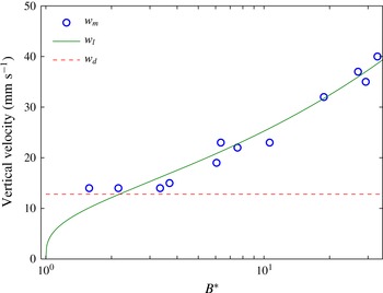
Figure 4 shows the measured maximum vertical velocity,
 $w_{m}$
, as a function of
 $B^{\ast }$
, as well as the predicted vertical velocity,
 $w_{l}$
, from the model of a wall plume from a line source of buoyancy (2.16) and the predicted velocity,
 $w_{d}$
, from the model of a wall plume from a distributed source of buoyancy (2.5).
 $w_{m}$
is measured after the velocity has approached a uniform value with height when possible, and at a height of approximately 0.8 m when the velocity does not reach a uniform value (e.g.
 $B^{\ast }=1.6$
on figure 3).
 $w_{l}$
is plotted based on
 $B_{s}$
, as the distributed source of buoyancy is expected to lead to a slow acceleration of the plume. In calculating
 $w_{l}$
, the drag coefficient,
 $c_{D}$
, is assumed to be negligible.
An entrainment coefficient of 0.075 is calculated based on the experimental data above
 $B^{\ast }=4$
. Data for
 $B^{\ast }<4$
are not used in calculating the entrainment coefficient, as the distributed buoyancy flux may have an important effect on the plume velocity in these experiments. The calculated entrainment coefficient is consistent with those described in § 2 from previous experimental studies, especially that measured by Sangras et al. (Reference Sangras, Dai and Faeth1999) at the largest heights. A result of using
 $B_{s}$
to calculate
 $w_{l}$
, is that
 $w_{l}=0$
for
 $B^{\ast }=1$
despite the real expected velocity being non-zero due to the buoyancy flux from the ice wall. The dashed line on figure 4 shows the vertical velocity for a wall plume from a distributed source of buoyancy,
 $w_{d}$
(McConnochie & Kerr Reference McConnochie and Kerr2016b
). The velocity is calculated based on a far-field temperature of
 $4.1\,^{\circ }\text{C}$
, a far-field salinity of 3.4 wt % NaCl and a height of 80 cm from the turbulent transition.
 $w_{d}$
represents a lower limit on what the measured velocity can be.
Figure 4 shows that for
 $B^{\ast }<2$
the distributed buoyancy source from the ice wall has an important effect on the plume velocity, but can be ignored for larger values of
 $B^{\ast }$
. For
 $B^{\ast }>2$
the model of a wall plume from a line source of buoyancy described in § 2 accurately predicts the plume velocity with an entrainment coefficient of 0.075.
4.2 Interface temperature
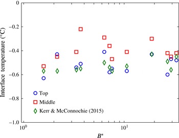
Figure 5 shows the interface temperature at two locations up the ice wall: ‘top’ and ‘middle’. These two locations reflect thermistor locations of 0.68 m and 0.43–0.50 m from the base of the tank, respectively. The typical difference between the two thermistors positioned 0.68 m above the base of the tank was used to assess a measurement uncertainty of
 $\pm 0.1\,^{\circ }\text{C}$
, which is reflected in the scatter of the data points. The interface temperature measured by Kerr & McConnochie (Reference Kerr and McConnochie2015) for a wall plume from a distributed source of buoyancy is shown with green diamonds. The variation between experiments is due to changes in the far-field fluid temperature.
The measured interface temperature,
 $T_{i}$
, as a function of
 $B^{\ast }$
. Two measurement locations are shown: ‘top’ shows the average of the two thermistors positioned 0.68 m above the base of the tank and ‘middle’ shows the average interface temperature from the thermistors 0.43, 0.50 and 0.55 m above the base of the tank. A predicted interface temperature is shown based on the experiments of Kerr & McConnochie (Reference Kerr and McConnochie2015) for a wall plume from a distributed source of buoyancy.

The interface temperature at both measurement locations is constant within experimental error over the full range of
 $B^{\ast }$
. The interface temperature is slightly higher in the middle region than at the top region, suggesting that the transport of heat relative to salt is less at lower heights.
Particularly at the ‘top’ location, the interface temperature is consistent with previous results without a source plume (Kerr & McConnochie Reference Kerr and McConnochie2015). This suggests that the relative transport of heat and salt to the ice is not significantly changed by the addition of an external plume beyond some initial transition distance. Based on (2.17), the plume buoyancy, and hence the plume temperature and salinity anomaly, should scale like
 $1/z$
, reflecting the rapid entrainment of ambient fluid. This rapid entrainment will lead to the wall plume quickly developing a similar temperature and salinity to the ambient fluid, irrespective of the source plume strength or properties. For example, at
 $B^{\ast }=7.6$
, the plume buoyancy will be approximately 1 % of that at the source after only 21 cm. This result shows that past theory and experiments (Kerr & McConnochie Reference Kerr and McConnochie2015) can be used to predict the interface conditions of a dissolving vertical ice face in the presence of an external plume, provided sufficient height for the plume to entrain enough ambient fluid that the source properties are unimportant.
4.3 Ablation velocity
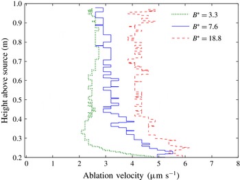
Figure 6 shows the measured ablation velocity as a function of height up the ice wall for three experiments with
 $B^{\ast }=3.3$
, 7.6 and 18.8. The height is measured from the source location, not the bottom of the tank. The two profiles for
 $B^{\ast }=7.6$
and 18.8 show the average ablation velocity from two photos taken 25 min apart from each other. For the profile at
 $B^{\ast }=3.3$
, the two photos were taken 50 min apart, due to the slower ablation rate. More photos were taken within this interval to confirm that the ablation rate was constant with time. The horizontal steps on the profile reflect the pixel size of the photographs which are the limit to our measurement resolution.
The measured ablation velocity,
 $V$
, as a function of height above the source for three typical experiments with
 $B^{\ast }=3.3$
, 7.6 and 18.8.

Throughout most of the tank the ablation velocity is near-uniform with height, as observed by Kerr & McConnochie (Reference Kerr and McConnochie2015) for the case of a distributed source of buoyancy (
 $B^{\ast }=1$
). We have not shown data from close to the source, as within this region the plume is becoming turbulent and then becoming attached to the ice wall. The attachment of the plume to the ice will significantly change the dissolution process, and occurs at a different location across experiments and while an experiment is being conducted. At the bottom of the profiles shown on figure 6, the ablation velocity is higher than the uniform value in the upper section of the tank.
The measured ablation velocity,
 $V$
, as a function of
 $B^{\ast }$
. Two measurement locations are shown, 0.80 m above the source location (blue circles) and 0.50 m above the source location (red squares). The three dashed lines show
 $V=1.5Q_{s}^{1/3}$
,
 $V=2Q_{s}^{1/3}$
and
 $V=2.5Q_{s}^{1/3}$
to represent the
 $V\sim Q_{s}^{1/3}$
scaling predicted by previous numerical investigations (Straneo & Cenedese Reference Straneo and Cenedese2015, and references therein).

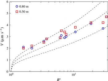
Figure 7 shows the ablation velocity as a function of
 $B^{\ast }$
. Measurements are shown for two heights that are both within the region of near-uniform ablation velocity shown on figure 6. For low values of
 $B^{\ast }$
, the ablation velocity is insensitive to changes in
 $B^{\ast }$
, while above
 $B^{\ast }\approx 3$
, the ablation velocity begins to increase with increasing
 $B^{\ast }$
. The three dashed lines show
 $V=1.5Q_{s}^{1/3}$
,
 $V=2Q_{s}^{1/3}$
and
 $V=2.5Q_{s}^{1/3}$
to show the
 $V\sim Q_{s}^{1/3}$
scaling predicted by previous numerical studies for line plumes (Straneo & Cenedese Reference Straneo and Cenedese2015). The scaling is seen to over-predict the increase in ablation velocity with
 $B^{\ast }$
for our experiments.
Across our experiments the ambient fluid temperature and salinity vary significantly. These changes in far-field conditions result in changes in the ablation velocity in addition to the changes caused by different values of
 $B^{\ast }$
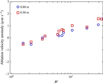
. To remove the effect of the changing far-field conditions we have subtracted the expected ablation velocity for a distributed source of buoyancy (Kerr & McConnochie Reference Kerr and McConnochie2015) from the data in figure 7. The resulting ablation anomaly is shown as a function of
 $B^{\ast }$
on figure 8.
The ablation velocity anomaly caused by the source plume as a function of
 $B^{\ast }$
. The expected ablation velocity from a distributed source of buoyancy (Kerr & McConnochie Reference Kerr and McConnochie2015) is subtracted from the measured ablation velocity shown in figure 7.

Figure 8 shows that, after the effect of varying far-field conditions is removed, the ablation velocity increases smoothly with
 $B^{\ast }$
. For
 $B^{\ast }<3$
, the ablation velocity appears to be decreased by the presence of a source plume. The reduction in ablation velocity is larger than the measurement uncertainty, so is not expected to be caused by experimental error. The line source of buoyancy introduces a salinity and temperature deficit to the wall plume. For high values of
 $B^{\ast }$
, the initial temperature and salinity deficit quickly decays due to turbulent entrainment of ambient fluid into the plume. However, at low values of
 $B^{\ast }$
, the wall plume is dominated by the distributed source of buoyancy rather than the line source of buoyancy (see § 4.1). The wall plume from a distributed source of buoyancy has a lower rate of entrainment, which could allow the salinity and temperature deficit to persist up the ice wall and lead to a reduced ablation rate.
For
 $B^{\ast }>3$
, the ablation velocity anomaly is positive and increases with increasing
 $B^{\ast }$
, as shown on figure 7. Considering the effect of varying far-field properties by subtracting the expected ablation velocity with a distributed buoyancy flux removes most of the experimental scatter in figure 7.
5 Oceanographic application
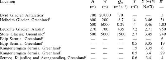
Table 2 gives estimated values of
 $B^{\ast }$
for a variety of tidewater glaciers. Two different methods have been used to calculate
 $B^{\ast }$
. For Byrd Glacier, Helheim Glacier, LeConte Glacier and Store Glacier, the subglacial discharge and the width over which it is released has been directly estimated (Motyka et al.
Reference Motyka, Hunter, Echelmeyer and Connor2003; Stearns, Smith & Hamilton Reference Stearns, Smith and Hamilton2008; Sciascia et al.
Reference Sciascia, Straneo, Cenedese and Heimbach2013; Xu et al.
Reference Xu, Rignot, Fenty and Menemenlis2013). This has been combined with an assumed ablation velocity of
 $3~\unicode[STIX]{x03BC}\text{m}~\text{s}^{-1}$
(see figure 7) in order to estimate
 $B^{\ast }$
. For Eqip Sermia, Kangerlerngata Sermia, Sermeq Kujatdleq and Sermeq Avangnandleq, the ratio of subglacial volume flux to meltwater volume flux was inferred based on measured water properties in front of the glacier (Rignot, Koppes & Velicogna Reference Rignot, Koppes and Velicogna2010; Beaird et al.
Reference Beaird, Straneo and Jenkins2015). This ratio of fluxes was used to calculate
 $B^{\ast }$
directly based on the assumption that the subglacial discharge was released uniformly over the entire width of the glacier. If the subglacial discharge was released from a more limited width (Fried et al.
Reference Fried, Catania, Bartholomaus, Duncan, Davis, Stearns, Nash, Shroyer and Sutherland2015), the resulting value of
 $B^{\ast }$
would be higher in regions where the subglacial flux per unit width was larger, and lower elsewhere.
Estimated values of glacier height,
 $H$
, subglacial discharge width,
 $W$
, subglacial volume flux,
 $Q_{sg}$
, ocean temperature,
 $T$
, ocean salinity,
 $S$
and
 $B^{\ast }$
for a variety of tidewater glaciers. Observations for Byrd Glacier were made during a sporadic subglacial lake drainage event while other observations are representative of summer conditions.
Observational data are from:
a Stearns et al. (Reference Stearns, Smith and Hamilton2008).
b Sciascia et al. (Reference Sciascia, Straneo, Cenedese and Heimbach2013).
c Motyka et al. (Reference Motyka, Hunter, Echelmeyer and Connor2003).
d Xu et al. (Reference Xu, Rignot, Fenty and Menemenlis2013).
e Beaird et al. (Reference Beaird, Straneo and Jenkins2015).
f Rignot et al. (Reference Rignot, Koppes and Velicogna2010).
Ocean temperature and salinity are given where available and are measured near the base of the glacier.
Over the seven locations in table 2,
 $B^{\ast }$
varies from an order of
 $10^{0}$
–
 $10^{3}$
. Most of the glaciers have a value of
 $B^{\ast }$
that is comparable to our experiments, with the exception of LeConte Glacier and Store Glacier. The values of
 $B^{\ast }$
given in table 2 for Alaskan and Greenlandic glaciers are representative of summer conditions only, and are expected to be highly seasonal. In winter, the subglacial volume flux will decrease and probably stop completely. At such times
 $B^{\ast }\approx 1$
, the ablation velocity will be as described by Kerr & McConnochie (Reference Kerr and McConnochie2015) and the plume velocity will be as described by (2.5). In the case of Byrd Glacier, the measured subglacial discharge was caused by the rapid draining of a subglacial lake, and was highly unusual. The hydrology beneath the Antarctic ice sheet is not well understood, but such events are rarely observed. As such, typical ablation velocities and plume velocities for Antarctic glaciers would be better described by Kerr & McConnochie (Reference Kerr and McConnochie2015) and (2.5), respectively.
There is a high degree of uncertainty in the calculated values of
 $B^{\ast }$
due to the difficulty in observing the subglacial discharge close to the ice face. In particular, the unknown discharge geometry means that assumptions are required to calculate the width over which the subglacial plume is released. Improved observations of these plumes close to the discharge location would lead to more accurate predictions of the impact that a subglacial plume may have on ice–ocean interactions in these regions.
There are also several physical processes that could be important in an oceanographic situation that are not included in our laboratory experiments. For example, the Coriolis force could alter the dynamics of the buoyant plume, the presence of stratification is likely to reduce the ablation rate and lead to double-diffusive intrusions into the ocean (McConnochie & Kerr Reference McConnochie and Kerr2016a
), and the pressure dependence on the freezing point of water will alter the ablation rate, possibly causing refreezing at shallow locations. In addition, the different spatial scales between the laboratory and the ocean could lead to altered dynamics. It is possible that the entrainment coefficient is dependent on the Reynolds number (Ellison & Turner Reference Ellison and Turner1959), which would be considerably larger next to tidewater glaciers. However, given that there is no evidence in the measurements of Sangras et al. (Reference Sangras, Dai and Faeth1999) and a similar entrainment coefficient is given in Jenkins (Reference Jenkins2011) based on field observations, we expect this dependence to be small. All of these processes complicate any comparison between our experiments and the glaciers that surround Greenland. Nonetheless, the values of
 $B^{\ast }$
given in table 2 suggest that the freshwater plume released at the base of Greenland glaciers in summer could enhance the ablation rate of these glaciers.
As previously noted, the salinity profiles in figure 2 have different shapes for high and low values of
 $B^{\ast }$
. As described in § 3, the peeling detrainment mechanism can be used to explain the lack of a density discontinuity observed at low values of
 $B^{\ast }$
(Hogg Reference Hogg2014; Hogg et al.
Reference Hogg, Dalziel, Huppert and Imberger2016). Glacial fjords are open ended to the ocean, so we would not expect a downward propagating layer of meltwater such as is observed in our experiments. In the absence of any peeling detrainment from the plume, we would instead expect the subglacial plume to either rise to the surface or to completely detach from the ice face and intrude at an intermediate depth of neutral buoyancy. In contrast, peeling detrainment would cause the plume to intrude over a range of depths and buoyancy levels.
Observations made by Beaird et al. (Reference Beaird, Straneo and Jenkins2015) in the fjord in front of Eqip Sermia and Kangerlerngata Sermia show meltwater both at the surface and within the upper 200 m of the fjord. In contrast, the subglacial discharge is almost completely limited to the upper 50 m of the water column. These observations are suggestive of peeling detrainment from the plume over a range of depths.
6 Conclusions
In this paper we have presented experiments that investigate the effect of an external cold freshwater plume on the dissolution of a vertical ice face. These experiments are intended to model conditions at the face of the many Greenland glaciers where subglacial plumes are frequently observed during summer months. Previous observations have shown that these subglacial plumes can lead to increased ablation rates, and as such could have a significant impact on the mass balance of the Greenland ice sheet. However, observations have had a limited capacity to explore how the ice–ocean interactions could be affected by altered subglacial fluxes.
The experiments have explored a range of source volume fluxes that bridge the region between a wall plume controlled by a vertically distributed buoyancy source and a wall plume controlled by a line source of buoyancy at the base of a wall. Our results generally show that an additional line source of buoyancy causes the plume velocity to increase (figure 4) and the ablation velocity to increase (figures 7 and 8) relative to the case of a wall plume from a distributed source of buoyancy (Kerr & McConnochie Reference Kerr and McConnochie2015; McConnochie & Kerr Reference McConnochie and Kerr2016b
). For small buoyancy fluxes (
 $B^{\ast }<3$
), the ablation velocity is slightly reduced. The interface temperature appears to be insensitive to the line source of buoyancy (figure 5). After an initial transition region, the plume velocity and the ablation velocity are both uniform with height.
A variety of oceanographic data near tidewater glaciers have been used to assess the relative importance of the subglacial buoyancy flux compared to the buoyancy flux derived from melting. Oceanographic measurements typically result in values of
 $B^{\ast }$
that are comparable to those from our experiments.
Acknowledgements
We gratefully acknowledge the technical assistance of B. Tranter, T. Beasley and A. Rummery, and the financial support of the Australian Research Council Discovery Grant DP120102772. We are also grateful to the reviewers who provided valuable suggestions throughout the review process.