1 Introduction
The dynamics of flows in natural systems is basically governed by exchanges between energies of different origin: kinetic, thermal, potential, magnetic, chemical… In the case of oceanic and atmospheric flows, the main energies involved are the kinetic energy and the potential energy (Vallis Reference Vallis2017). Understanding the interplay between the energy fluxes of these quantities, and their scaling properties is one of the main issue for climate modelling. The paradigm to study these issues is the Rayleigh–Bénard (RB) system in which solutions of the Boussinesq equations describe the movements of velocity  $u$ and temperature
 $T$ of a fluid heated from below. Even restricting ourselves to this configuration, many open issues remain to be addressed (Ahlers, Grossmann & Lohse Reference Ahlers, Grossmann and Lohse2009; Lohse & Xia Reference Lohse and Xia2010; Chillà & Schumacher Reference Chillà and Schumacher2012). We shall focus here on some properties of small scales, describing a new approach to analysing scaling behaviour and more generally fluctuation properties.
In realistic conditions, the energy is injected in such systems at large scales under the shape of potential energy, converted into kinetic energy and cascaded towards smaller scales by nonlinear interactions. At scales smaller than the global inhomogeneity scale, such dynamics can be regarded to occur via globally self-similar processes, with scaling laws that depend upon the parameters and the scale (Monin & Yaglom Reference Monin and Yaglom1975). In this problem, several characteristic scales have been identified other than the large scale typical of stratification: (i) The kinetic viscous or Kolmogorov scale  $\unicode[STIX]{x1D702}$; this scale corresponds to the scale at which the local Reynolds number is of order one. Below such a scale, the statistics of the velocity field are smooth, that is, the velocity increments
 $\unicode[STIX]{x1D6FF}u_{\ell }=|\boldsymbol{u}(x+r)-u(x)|$ scale statistically like
 $\ell$. (ii) The thermal viscous, or Batchelor scale
 $\unicode[STIX]{x1D702}_{T}$, corresponding in the same way to the scale at which thermal diffusion becomes dominant. Below such a scale, the statistics of the temperature field are smooth, that is, temperature increments
 $\unicode[STIX]{x1D6FF}T_{\ell }=T(x+\ell )-T(x)$ scale statistically like
 $\ell$. (iii) The Bolgiano–Oboukhov (BO) scale
 $L_{BO}$, which is the scale at which buoyancy effects become important and they may balance with dissipative terms. Below such a scale, the temperature is usually considered as ‘passive’, with negligible influence on the velocity field. Empirically, the sign, magnitude and scaling of the energy fluxes depend on how these scales are interlinked.
According to the prediction based on a generalization of the Kolmogorov theory for turbulent fluids, first suggested for stably stratified flows (Bolgiano Reference Bolgiano1959; Oboukhov Reference Oboukhov1959), the velocity and temperature increments scale like  $\unicode[STIX]{x1D6FF}u_{\ell }\sim \ell ^{1/5},\unicode[STIX]{x1D6FF}T_{\ell }\sim \ell ^{3/5}$ above
 $L_{BO}$, resulting in a constant flux of potential energy
 $\unicode[STIX]{x2202}_{\ell }\langle \unicode[STIX]{x1D6FF}u_{\ell }(\unicode[STIX]{x1D6FF}T_{\ell })^{2}\rangle$ towards the small scale. In contrast, for scale
 $\ell <L_{BO}$, the kinetic energy flux
 $\unicode[STIX]{x2202}_{\ell }\langle \unicode[STIX]{x1D6FF}u_{\ell }(\unicode[STIX]{x1D6FF}u_{\ell })^{2}\rangle$ is constant, so that
 $\unicode[STIX]{x1D6FF}u_{\ell }\sim \ell ^{1/3}$. Unfortunately, several issues make difficult the measurement of the BO scaling in a closed domain (Lohse & Xia Reference Lohse and Xia2010). In particular,
 $L_{BO}$ has been found to be globally of the order of the entire volume of the box, and the anisotropy could also make it ambiguous to discern between the BO scaling and other shear scalings (Biferale & Procaccia Reference Biferale and Procaccia2005). Moreover, the similarity argument does not take into account intermittency effect, produced by large fluctuations of velocity gradients or temperature gradients. Indeed, it is well known that both velocity and temperature are highly intermittent random fields (Benzi et al. Reference Benzi, Tripiccione, Massaioli, Succi and Ciliberto1994; Cioni, Ciliberto & Sommeria Reference Cioni, Ciliberto and Sommeria1995; Lohse & Xia Reference Lohse and Xia2010), and therefore local dynamics or local energy exchange may be subject to intense fluctuations and strong inhomogeneity.
Still it is important to observe that the system is non-homogeneous, because of the presence of the horizontal plates and lateral vertical sidewalls. That makes  $L_{BO}$ also a non-homogeneous quantity, which has been shown to vary its value over approximately one order of magnitude depending on the distance from the walls, both the top–bottom and the lateral ones (Calzavarini, Toschi & Tripiccione Reference Calzavarini, Toschi and Tripiccione2002; Kunnen et al. Reference Kunnen, Clercx, Geurts, van Bokhoven, Akkermans and Verzicco2008; Kaczorowski & Xia Reference Kaczorowski and Xia2013). For this reason, the presence of a BO scaling seems plausible, possibly over a tiny range. An important issue, common to other non-homogeneous flows, is the difficulty of computing an accurate scaling. The goal of the present work is to deal with this issue, presenting a new approach that allows us to access the local scaling.
Generally speaking, valuable information about the cascade ranges and the scaling laws of turbulent flows are found by measuring the spectrum of a flow. The same content is brought by the second-order structure function, notably employed in numerical simulations. Higher-order structure functions convey more refined information, notably about intermittency (Frisch Reference Frisch1995). Those are the tools also used to analyse small-scale behaviour in RB convection (Lohse & Xia Reference Lohse and Xia2010). On the one hand, structure functions are very noisy, even at the lowest level of second order, and it is difficult to obtain a clear scaling (Benzi, Toschi & Tripiccione Reference Benzi, Toschi and Tripiccione1998; Calzavarini et al. Reference Calzavarini, Toschi and Tripiccione2002; Kaczorowski & Xia Reference Kaczorowski and Xia2013). It is possible to improve the predictions using a particular fitting procedure known as ESS (extended self-similarity) (Benzi et al. Reference Benzi, Ciliberto, Tripiccione, Baudet, Massaioli and Succi1993). In this case, the ratio between the scaling exponent of different-order structure functions can be accessed more neatly. While this procedure has been effective in homogeneous isotropic turbulence, where the third-order structure function is known analytically (Frisch Reference Frisch1995), it gives only relative exponents in non-homogeneous flows like RB. On the other hand, the most common method to measure the spectrum is using Fourier transforms, notably in experiments, and Fourier techniques are inherently global in space and cannot characterize the flow properties locally. Yet the local properties seem to play a crucial role in non-homogeneous flows. The purpose of the present work is to put forward an approach capable of capturing the full complexity of local energy fluxes and exchanges. This is valuable for non-homogeneous flows like the RB convection for the inherent multiscale character of such a flow, as the production, transport and dissipation of energy depend on the position in space and on the scale considered.
As discussed in Dubrulle (Reference Dubrulle2019), a suitable framework is the weak formulation of the basic equations, via appropriate wavelet transforms. Technically, a main advantage wavelets have over Fourier analysis is the identification of flow properties simultaneously as a function of scale and space. For this reason wavelets have already proved their utility to access local scaling in turbulent flows (Meneveau Reference Meneveau1991; Farge Reference Farge1992; Jaffard, Meyer & Ryan Reference Jaffard, Meyer and Ryan2001) and most notably the multifractal spectrum (Kestener & Arneodo Reference Kestener and Arneodo2004). More generally, the weak approach is related the coarse-grained or filtered equations already developed for homogeneous turbulence (Duchon & Robert Reference Duchon and Robert2000; Eyink & Sreenivasan Reference Eyink and Sreenivasan2006), and it constitutes the most general framework to apply a scale-by-scale analysis to general non-homogeneous flows.
In a recent paper (Faranda et al. Reference Faranda, Lembo, Iyer, Kuzzay, Chibbaro, Daviaud and Dubrulle2018), we have implemented such a framework on the stably stratified Boussinesq equations, and derived the scale-by-scale equations for potential, kinetic and viscous energy fluxes. A preliminary yet encouraging analysis has then been made of some atmospheric data. By construction, the atmospheric data only provide a fragmented view of the energy fluxes, because they do not extend all the way to the viscous scales, where the extremes of kinetic energy flux are found to happen (Saw et al. Reference Saw, Kuzzay, Faranda, Guittonneau, Daviaud, Wiertel-Gasquet, Padilla and Dubrulle2016). In the present paper, we therefore apply the analysis to a more controlled and cleaner system, provided by numerical solutions of the Boussinesq equations at high resolution.
The paper is organized as follows: in § 2, we first recall the theoretical model and the numerical method. In § 3, we describe the theoretical framework and tools. In § 4, we provide the results and we discuss them. Finally we draw conclusions.
2 Governing equations and numerical method
We consider a turbulent Rayleigh–Bénard convection, in which a horizontal fluid layer is heated from below. Horizontal and wall-normal coordinates are indicated by  $x$,
 $y$ and
 $z$, respectively. Using the Boussinesq approximation, the system is described by the following dimensionless balance equations
 $$\begin{eqnarray}\displaystyle & \displaystyle \frac{\unicode[STIX]{x2202}u_{i}}{\unicode[STIX]{x2202}x_{i}}=0, & \displaystyle\end{eqnarray}$$
 $$\begin{eqnarray}\displaystyle & \displaystyle \frac{\unicode[STIX]{x2202}u_{i}}{\unicode[STIX]{x2202}t}+u_{j}\frac{\unicode[STIX]{x2202}u_{i}}{\unicode[STIX]{x2202}x_{j}}=-\frac{\unicode[STIX]{x2202}P}{\unicode[STIX]{x2202}x_{i}}+\sqrt{\frac{Pr}{Ra}}\frac{\unicode[STIX]{x2202}^{2}u_{i}}{\unicode[STIX]{x2202}x_{j}^{2}}+\unicode[STIX]{x1D6FF}_{i,3}\unicode[STIX]{x1D703}, & \displaystyle\end{eqnarray}$$
 $$\begin{eqnarray}\displaystyle & \displaystyle \frac{\unicode[STIX]{x2202}\unicode[STIX]{x1D703}}{\unicode[STIX]{x2202}t}+u_{j}\frac{\unicode[STIX]{x2202}\unicode[STIX]{x1D703}}{\unicode[STIX]{x2202}x_{j}}=\frac{1}{\sqrt{PrRa}}\frac{\unicode[STIX]{x2202}^{2}\unicode[STIX]{x1D703}}{\unicode[STIX]{x2202}x_{j}^{2}}, & \displaystyle\end{eqnarray}$$
where  $u_{i}$ is the
 $i$th component of the velocity vector,
 $P$ is pressure,
 $\unicode[STIX]{x1D703}=(T-T_{0})/\unicode[STIX]{x0394}T$ is the dimensionless temperature,
 $\unicode[STIX]{x0394}T=T_{H}-T_{C}$ is the imposed temperature difference between the hot bottom wall (
 $T_{H}$) and top cold wall (
 $T_{C}$),
 $T_{0}=(T_{C}+T_{H})/2$, whereas
 $\unicode[STIX]{x1D6FF}_{1,3}\unicode[STIX]{x1D703}$ is the driving buoyancy force (acting in the vertical direction
 $z$ only). The reference velocity is
 $u_{ref}=(g\unicode[STIX]{x1D6FD}H\unicode[STIX]{x0394}T)^{1/2}$, with
 $H$ the domain height,
 $g$ the acceleration due to gravity and
 $\unicode[STIX]{x1D6FD}$ the thermal expansion coefficient. The Prandtl and the Rayleigh numbers in equations (2.2)–(2.3) are defined as
 $Pr=\unicode[STIX]{x1D708}/\unicode[STIX]{x1D705}$ and
 $Ra=(g\unicode[STIX]{x1D6FD}\unicode[STIX]{x0394}TH^{3})/(\unicode[STIX]{x1D708}k)$, with
 $\unicode[STIX]{x1D708}$ the fluid kinematic viscosity and
 $\unicode[STIX]{x1D705}$ the thermal diffusivity.
Two direct numerical simulations (DNS) are performed for a fixed  $Pr=1$ at
 $Ra=10^{7}$ and
 $10^{8}$ in a cubic box of size
 $H^{3}$ with the
 $x$–
 $y$ plane parallel to the horizontal plates and the
 $z$ axis pointing in the direction opposite to that of gravitational acceleration. For the velocity, no-slip boundary conditions are used everywhere, as in experiments. For the temperature, adiabatic conditions are imposed at all lateral sidewalls whereas isothermal conditions are used on the top and bottom plates. Table 1 reports the main parameters of the simulations. Previous studies indicate that the BO scaling might be more clearly observable at the moderate
 $Ra$ numbers chosen here (Lohse & Xia Reference Lohse and Xia2010). In order to make the scaling neater, it would be in principle helpful to use higher Prandtl numbers (Kaczorowski & Xia Reference Kaczorowski and Xia2013). However, the dependence is very slow and the computational effort needed to keep the present accuracy at much higher
 $Pr$ numbers very important. For this first study concerning the weak approach to turbulent convection we have thus preferred use the somewhat standard
 $Pr=1$.
Equations (2.2)–(2.3) are solved through the open-source code Basilisk (see http://www.basilisk.fr/). In particular, space is discretized using a Cartesian (multi-level or tree-based) grid where the variables are located at the centre of each control volume (a square in two dimensions, a cube in three dimensions) and at the centre of each control surface.
Second-order finite-volume numerical schemes for the spatial gradients are used (Popinet Reference Popinet2003, Reference Popinet2009; Lagrée, Staron & Popinet Reference Lagrée, Staron and Popinet2011). Navier–Stokes equations are integrated by a projection method (Chorin Reference Chorin1969), and time advancing is performed through a fractional-step method using a staggered discretization in time of the velocity and the scalar fields (Popinet Reference Popinet2009).
Some remarks are in order concerning the numerical method. From a numerical point of view, it is worth noting that our upwind method is actually third order in space when considering the advection term. The Basilisk code has been tested in isotropic turbulence and in particular compared with a finite-volume scheme which preserves energy (Fuster Reference Fuster2013). The results are in good agreement with those obtained with a spectral code and no difference is encountered between the two finite-volume methods, whenever the resolution is sufficient to resolve all scales (http://www.basilisk.fr/). The code has been recently used and extensively validated in RB turbulent convection (Castillo-Castellanos, Sergent & Rossi Reference Castillo-Castellanos, Sergent and Rossi2016; Castillo-Castellanos Reference Castillo-Castellanos2017; Castillo-Castellanos et al. Reference Castillo-Castellanos, Sergent, Podvin and Rossi2019). In this thorough validation, it has been shown that, provided the requirements on the resolution are respected (Stevens, Verzicco & Lohse Reference Stevens, Verzicco and Lohse2010; Shishkina et al. Reference Shishkina, Stevens, Grossmann and Lohse2010), no appreciable difference can be found with respect to the literature with respect to any observable. Furthermore, in a recent work, the numerical approach has been assessed in a one-to-one comparison against a standard code also in the case of an atmospheric boundary layer. The results are satisfying in all respects and numerical dissipation appears to be ineffective, provided the resolution is sufficient to well resolve the boundary layer (van Hooft et al. Reference van Hooft, van Heerwaarden, Popinet, de Roode and van de Wiel2017).
List of the dimensionless parameters,  $Ra$ and
 $Pr$, for the different test runs, and the parameters of the simulations: the number of grid points
 $N_{x}\times N_{y}\times N_{z}$ in the respective spatial directions; the number of grid points required for resolution of the thermal boundary layer
 $N_{T}$ (requirement/actual resolution); the requirement is based on the analysis in Stevens et al. (Reference Stevens, Verzicco and Lohse2010) and Shishkina et al. (Reference Shishkina, Stevens, Grossmann and Lohse2010). The mean heat transfer computed with the three different formulas:
 $Nu\equiv 1+\sqrt{RaPr}\langle u_{z}T\rangle ,Nu_{\unicode[STIX]{x1D716}_{u}}\equiv 1+\sqrt{RaPr}\langle \unicode[STIX]{x1D716}_{u}\rangle$ and
 $Nu_{\unicode[STIX]{x1D716}_{T}}\equiv \sqrt{RaPr}\langle \unicode[STIX]{x1D716}_{T}\rangle$, where
 $\langle \,\rangle$ indicates averaging, and the statistics have been computed averaging in space over the entire volume and over
 $300$ reference times.

We have chosen a horizontal ( $N_{x},N_{y}$) and vertical (
 $N_{z}$) number of points sufficiently large to solve the smallest length scale of the problem, which is the Kolmogorov length scale
 $\unicode[STIX]{x1D702}=(\unicode[STIX]{x1D708}^{3}/\langle \unicode[STIX]{x1D716}\rangle )^{1/4}$, since
 $Pr=1$ in all regions. Moreover, we have checked that we fulfil the criteria proposed for RB convection to ensure proper resolution of the thermal dynamics (Shishkina et al. Reference Shishkina, Stevens, Grossmann and Lohse2010). Although this particular resolution is only required near to the wall, we have chosen to use a uniform grid since we are interested in monitoring the fluctuations in the centre of the cube, where vertical non-homogeneity is less important. For this reason, and given the geometry chosen, the grid spacing is the same in all directions
 $\unicode[STIX]{x1D6E5}_{x}=\unicode[STIX]{x1D6E5}_{y}=\unicode[STIX]{x1D6E5}_{z}=\unicode[STIX]{x1D6E5}=1/1024$. The Kolmogorov length scale
 $\unicode[STIX]{x1D702}$ is computed a posteriori from the datasets via spatial and time average. As shown in table 1, for both of the DNS, the value of the Kolmogorov length scale is much larger than the grid spacing, so that we are over-resolving the flow (Verzicco & Camussi Reference Verzicco and Camussi2003). Moreover, as shown in the same table 1, the resolution greatly exceeds also the requirements for the thermal layers, notably at lower Rayleigh number. That was a deliberate choice for two reasons: (i) Basilisk is a volume-finite code which may add some numerical diffusion at the smallest scales. Since we are precisely interested in the behaviour at small scales, we use a resolution higher than necessary to avoid spurious effects. (ii) We are also interested in the possible presence of extreme events at very small scales,
 $\ell \sim \unicode[STIX]{x1D702}$, and therefore we have carried out simulations with a resolution much higher than usual to be sure to well resolve all the scales
 $\ell \lesssim \unicode[STIX]{x1D702}$.
After the initial transient, velocity and temperature fields are collected with a time interval significantly longer than the large eddy turnover time  $2h/u_{ref}$ in order to ensure that the fields are uncorrelated. The statistical convergence has been checked by looking at different statistics and observing that the average mean field is zero. In order to assess the resolution of the numerical method, we show in table 1 also the consistency relation for the mean heat transfer (Siggia Reference Siggia1994; Verzicco & Camussi Reference Verzicco and Camussi2003):
 $Nu\equiv 1+\sqrt{RaPr}\langle u_{3}\unicode[STIX]{x1D703}\rangle =Nu_{\unicode[STIX]{x1D716}}\equiv 1+\sqrt{RaPr}\langle \unicode[STIX]{x1D716}\rangle =Nu_{\unicode[STIX]{x1D716}_{T}}\equiv \sqrt{RaPr}\langle \unicode[STIX]{x1D716}_{T}\rangle$, where
 $\langle \,\rangle$ indicates ensemble averaging,
 $\unicode[STIX]{x1D716}$ is the dissipation rate and
 $\unicode[STIX]{x1D716}_{T}$ is the temperature variance dissipation rate. The results are indeed consistent and in agreement with the values from the literature for both
 $Ra$ numbers (Ahlers et al. Reference Ahlers, Grossmann and Lohse2009).
3 Weak formulation
3.1 Summary of local energy budget
In this section, we present the local energy budget of Boussinesq equations (2.2)–(2.3), which relies on the weak formulation of the equations (Duchon & Robert Reference Duchon and Robert2000) and has been derived in a recent work (Faranda et al. Reference Faranda, Lembo, Iyer, Kuzzay, Chibbaro, Daviaud and Dubrulle2018) for the case of stably stratified flows. Although we deal with unstable stratification in this work, the derivation is the same and we refer to that reference for the details. The local budget involves the filtered or coarse-grained observable  $\widetilde{o}_{\ell }$ defined as
 $$\begin{eqnarray}\widetilde{o}_{\ell }(x,t)\equiv \int d^{d}rG_{\ell }(r)o(x+r,t),\end{eqnarray}$$
where the subscript  $\ell$ refers to the scale dependence introduced by the filtering. The filter
 $G$ is a smooth function, non-negative, spatially localized and such that
 $\int \text{d}\boldsymbol{r}\,G(\boldsymbol{r})=1$, and
 $\int \text{d}\boldsymbol{r}\,|\boldsymbol{r}|^{2}G(\boldsymbol{r})\approx 1$. The function
 $G_{\ell }$ is rescaled with
 $\ell$ as
 $G_{\ell }(\boldsymbol{r})=\ell ^{-3}G(\boldsymbol{r}/\ell )$. At a given finite scale
 $\ell$, the local energy budget depends on this filtering, but all the results obtained in the limit
 $\ell \rightarrow 0$ are independent of
 $G$. In the sequel, we take
 $G$ as a Gaussian whenever analysing the numerical data. The local scale-by-scale equations for the energy and temperature variance read as (Faranda et al. Reference Faranda, Lembo, Iyer, Kuzzay, Chibbaro, Daviaud and Dubrulle2018):
 $$\begin{eqnarray}\displaystyle & & \displaystyle \unicode[STIX]{x2202}_{t}\left(\frac{1}{2}\boldsymbol{u}\boldsymbol{\cdot }\widetilde{\boldsymbol{u}}_{\ell }\right)+\unicode[STIX]{x1D735}\boldsymbol{\cdot }\left[\frac{1}{2}(\boldsymbol{u}\boldsymbol{\cdot }\widetilde{\boldsymbol{u}}_{\ell })\boldsymbol{u}+\frac{1}{2}(p\widetilde{\boldsymbol{u}}_{\ell }+\widetilde{p}_{\ell }\boldsymbol{u})+\frac{1}{4}\widetilde{(|\boldsymbol{u}|^{2}\boldsymbol{u})}_{\ell }\right.\nonumber\\ \displaystyle & & \displaystyle \qquad -\left.\frac{1}{4}\widetilde{(|\boldsymbol{u}|^{2})}_{\ell }\boldsymbol{u}-\frac{1}{2}\sqrt{\frac{Pr}{Ra}}\unicode[STIX]{x1D735}(\widetilde{\boldsymbol{u}_{\ell }}\boldsymbol{\cdot }\boldsymbol{u})\right]=-\frac{1}{4}\int d^{d}r\unicode[STIX]{x1D735}G_{\ell }\boldsymbol{\cdot }\unicode[STIX]{x1D6FF}\boldsymbol{u}_{\ell }|\unicode[STIX]{x1D6FF}\boldsymbol{u}_{\ell }|^{2}\nonumber\\ \displaystyle & & \displaystyle \qquad -\,\sqrt{\frac{Pr}{Ra}}\int d^{d}r\unicode[STIX]{x1D6FB}^{2}G_{\ell }|\unicode[STIX]{x1D6FF}\boldsymbol{u}_{\ell }|^{2}+\frac{1}{2}(u_{3}\widetilde{\unicode[STIX]{x1D703}}_{\ell }+\widetilde{u}_{3\ell }\unicode[STIX]{x1D703})\nonumber\\ \displaystyle & & \displaystyle \quad \equiv -\text{D}_{\ell }-\text{D}_{\ell }^{\unicode[STIX]{x1D708}}+\text{D}_{\ell }^{c},\end{eqnarray}$$
and
 $$\begin{eqnarray}\displaystyle & & \displaystyle \unicode[STIX]{x2202}_{t}\left(\frac{1}{2}\unicode[STIX]{x1D703}\widetilde{\unicode[STIX]{x1D703}}_{\ell }\right)+\unicode[STIX]{x1D735}\boldsymbol{\cdot }\left[\frac{1}{2}(\boldsymbol{u}\boldsymbol{\cdot }\widetilde{\unicode[STIX]{x1D703}}_{\ell })\unicode[STIX]{x1D703}+\frac{1}{4}\widetilde{(\unicode[STIX]{x1D703}^{2}\boldsymbol{u})}_{\ell }-\frac{1}{4}\widetilde{(\unicode[STIX]{x1D703}^{2})}_{\ell }\boldsymbol{u}-\frac{1}{2\sqrt{RaPr}}\unicode[STIX]{x1D735}(\unicode[STIX]{x1D703}\widetilde{\unicode[STIX]{x1D703}_{\ell }})\right]\nonumber\\ \displaystyle & & \displaystyle \quad =-\frac{1}{4}\int d^{d}r\unicode[STIX]{x1D735}G_{\ell }\boldsymbol{\cdot }\unicode[STIX]{x1D6FF}\boldsymbol{u}_{\ell }(\unicode[STIX]{x1D6FF}\unicode[STIX]{x1D703})^{2}-\frac{1}{\sqrt{PrRa}}\int d^{d}r\unicode[STIX]{x1D6FB}^{2}G_{\ell }|\unicode[STIX]{x1D6FF}\unicode[STIX]{x1D703}_{\ell }|^{2}\nonumber\\ \displaystyle & & \displaystyle \quad \equiv -\text{D}_{\ell }^{T}-\text{D}_{\ell }^{\unicode[STIX]{x1D705}},\end{eqnarray}$$
where  $\unicode[STIX]{x1D6FF}\unicode[STIX]{x1D703}_{\ell }$ and
 $\unicode[STIX]{x1D6FF}\boldsymbol{u}_{\ell }$ are, respectively, the temperature and velocity increments defined in § 1.
All the budget terms denoted by  $\text{D}$ are implicitly defined by the equations, as indicated by the symbol
 $\equiv$. In particular, in (3.2),
 $\text{D}_{\ell }$ is related to the inertial dissipation,
 $\text{D}_{\ell }^{\unicode[STIX]{x1D708}}$ represents the viscous dissipation and
 $\text{D}_{\ell }^{c}$ the coupling term. In equation (3.3),
 $\text{D}_{\ell }^{T}$ is the inertial dissipation term for the temperature variance and
 $\text{D}_{\ell }^{\unicode[STIX]{x1D705}}$ represents the viscous diffusion.
As discussed in Faranda et al. (Reference Faranda, Lembo, Iyer, Kuzzay, Chibbaro, Daviaud and Dubrulle2018) and Dubrulle (Reference Dubrulle2019), and shown below, these equations are a local fluctuating form of the Kármán–Howarth–Monin (KHM) equations (Monin & Yaglom Reference Monin and Yaglom1975), including the exchange term between temperature and velocity due to buoyancy. As typical for non-equilibrium macroscopic phenomena, the kinetic or thermal energy  $\unicode[STIX]{x2202}_{t}(\frac{1}{2}\boldsymbol{u}\boldsymbol{\cdot }\boldsymbol{u}_{\ell })$ or
 $\unicode[STIX]{x2202}_{t}(\frac{1}{2}\unicode[STIX]{x1D703}\widetilde{\unicode[STIX]{x1D703}}_{\ell })$ evolves through (i) a current describing mean transport via a spatial flux; (ii) a local term related to the exchange of energy at the scale
 $\ell$, (iii) a local sink term due to (viscous or thermal) dissipation and (iv) a local term linked to the buoyancy work that redistributes the energy between the thermal and the kinetic part.
As conjectured by Onsager (Onsager Reference Onsager1949; Eyink & Sreenivasan Reference Eyink and Sreenivasan2006) and rigorously stated by Duchon & Robert (Reference Duchon and Robert2000), the nonlinear inter-scale term  $\text{D}_{\ell }$ converges to the inertial dissipation term at infinite Reynolds number in the asymptotic small-scale limit
 $$\begin{eqnarray}\text{D}=\lim _{\ell \rightarrow 0}(\lim _{\unicode[STIX]{x1D708}\rightarrow 0}\text{D}_{\ell }).\end{eqnarray}$$
In this limit, the nonlinear terms may dissipate energy, when the field is sufficiently irregular (Duchon & Robert Reference Duchon and Robert2000). In the same way, we define
 $$\begin{eqnarray}\text{D}^{T}=\lim _{\ell \rightarrow 0}\text{D}_{\ell }^{T};\quad \text{D}^{\unicode[STIX]{x1D708}}=\lim _{\ell \rightarrow 0}\text{D}_{\ell }^{\unicode[STIX]{x1D708}};\quad \text{D}^{\unicode[STIX]{x1D705}}=\lim _{\ell \rightarrow 0}\text{D}_{\ell }^{\unicode[STIX]{x1D705}};\quad \text{D}^{c}=\lim _{\ell \rightarrow 0}\text{D}_{\ell }^{c}.\end{eqnarray}$$
Furthermore, in the average sense we have the relation
 $$\begin{eqnarray}\langle \text{D}^{\unicode[STIX]{x1D708}}\rangle \equiv {\mathcal{D}}^{\unicode[STIX]{x1D708}}=\unicode[STIX]{x1D716},\quad \text{with }\unicode[STIX]{x1D716}=\langle \unicode[STIX]{x1D708}|\unicode[STIX]{x1D735}\boldsymbol{u}|^{2}\rangle ,\end{eqnarray}$$
and
 $$\begin{eqnarray}\langle \text{D}^{\unicode[STIX]{x1D705}}\rangle \equiv {\mathcal{D}}^{\unicode[STIX]{x1D705}}=\unicode[STIX]{x1D716}_{T},\quad \text{with }\unicode[STIX]{x1D716}_{T}=\langle \unicode[STIX]{x1D705}|\unicode[STIX]{x1D735}\unicode[STIX]{x1D703}|^{2}\rangle ;\end{eqnarray}$$
where  $\langle \,\rangle$ denotes spatial and time average. In the same way we have
 $$\begin{eqnarray}\langle \text{D}^{c}\rangle \equiv {\mathcal{D}}^{c}=(Nu-1)/\sqrt{RaPr},\quad \text{with }(Nu-1)/\sqrt{RaPr}=\langle u_{3}\unicode[STIX]{x1D703}\rangle .\end{eqnarray}$$
On the other hand, whenever  $\boldsymbol{u}$ and
 $\unicode[STIX]{x1D703}$ are regular, we have in the limit
 $\ell \rightarrow 0$,
 $\unicode[STIX]{x1D6FF}u_{\ell }\sim \ell$ and
 $\unicode[STIX]{x1D6FF}\unicode[STIX]{x1D703}_{\ell }\sim \ell$, so that both
 $\text{D}$ and
 $\text{D}^{T}$ scale like
 $\ell ^{2}$ and tend to zero. The location where these quantities do not converge to zero is the location of potential quasi-singularities (Dubrulle Reference Dubrulle2019) that will be studied elsewhere. Empirically, we observe that these points are very rare, so that, on average, we have
 $\langle \text{D}\rangle =\langle \text{D}\rangle ^{T}=0$. The way in which these limits are achieved is, however, informative in terms of the scaling properties of the flow, as is shown in § 3.4. When averaged, equations (3.2)–(3.3) give the general forms of the mean energy and temperature budgets, and they are interesting since they provide a scale-by-scale way to analyse turbulent flows, as highlighted in several recent works focused on anisotropic turbulent flows (Hill Reference Hill1997; Danaila et al. Reference Danaila, Anselmet, Zhou and Antonia1999; Rincon Reference Rincon2006; Cimarelli, De Angelis & Casciola Reference Cimarelli, De Angelis and Casciola2013; Gauding et al. Reference Gauding, Wick, Pitsch and Peters2014; Togni, Cimarelli & De Angelis Reference Togni, Cimarelli and De Angelis2015; Mollicone et al. Reference Mollicone, Battista, Gualtieri and Casciola2018).
3.2 Global energy budget and Yaglom equations
By taking ensemble averages of the equations (3.2) and (3.3), we can thus obtain a global scale-dependent energy budget. Considering a stationary state, and taking into account the contribution of the spatial flux terms due to the temperature boundary condition, we then obtain
 $$\begin{eqnarray}\displaystyle \left.\begin{array}{@{}c@{}}\displaystyle \frac{1}{2}\langle \boldsymbol{u}\widetilde{\unicode[STIX]{x1D703}}_{\ell }+\widetilde{\boldsymbol{u}}_{\ell }\unicode[STIX]{x1D703}\rangle =\frac{1}{4}\int d^{d}r\unicode[STIX]{x1D735}G_{\ell }\boldsymbol{\cdot }\langle \unicode[STIX]{x1D6FF}\boldsymbol{u}(r)|\unicode[STIX]{x1D6FF}\boldsymbol{u}(r)|^{2}\rangle +\sqrt{\frac{Pr}{Ra}}\int d^{d}r\unicode[STIX]{x1D6FB}^{2}G_{\ell }\langle \unicode[STIX]{x1D6FF}(\boldsymbol{u}(r))^{2}\rangle ,\\ \displaystyle \oint _{\unicode[STIX]{x2202}V}J_{\ell }^{T}d\unicode[STIX]{x1D6F4}=\frac{1}{4}\int d^{d}r\unicode[STIX]{x1D735}G_{\ell }\boldsymbol{\cdot }\langle \unicode[STIX]{x1D6FF}\boldsymbol{u}(r)(\unicode[STIX]{x1D6FF}\unicode[STIX]{x1D703})^{2}\rangle +\frac{1}{\sqrt{PrRa}}\int d^{d}r\unicode[STIX]{x1D6FB}^{2}G_{\ell }\langle (\unicode[STIX]{x1D6FF}\unicode[STIX]{x1D703}(r))^{2}\rangle ,\end{array}\!\right\}\qquad & & \displaystyle\end{eqnarray}$$
where  $J_{\ell }^{T}=[\frac{1}{2}(\boldsymbol{u}\boldsymbol{\cdot }\widetilde{\unicode[STIX]{x1D703}}_{\ell })\unicode[STIX]{x1D703}+\frac{1}{4}\widetilde{(\unicode[STIX]{x1D703}^{2}\boldsymbol{u})}_{\ell }-\frac{1}{4}\widetilde{(\unicode[STIX]{x1D703}^{2})}_{\ell }\boldsymbol{u})-1/(2\sqrt{RaPr})\unicode[STIX]{x1D735}(\unicode[STIX]{x1D703}\widetilde{\unicode[STIX]{x1D703}_{\ell }})]$. It is worth noting that in the present work statistical averages will be computed through spatial and time averaging, thanks to the stationarity of the flow and by using the Ergodic hypothesis.
In the limit  $\ell \rightarrow 0$, we have
 $\oint J_{\ell }^{T}d\unicode[STIX]{x1D6F4}\rightarrow -Nu/\sqrt{RaPr}$ so that the global energy budget yields
 $$\begin{eqnarray}\displaystyle \left.\begin{array}{@{}c@{}}(Nu-1)/\sqrt{RaPr}=\langle \text{D}\rangle +\unicode[STIX]{x1D716},\\ Nu/\sqrt{RaPr}=\langle \text{D}\rangle ^{T}+\unicode[STIX]{x1D716}_{T}.\end{array}\right\} & & \displaystyle\end{eqnarray}$$
Taking into account  $\langle \text{D}\rangle =\langle \text{D}\rangle ^{T}=0$, we then get
 $\unicode[STIX]{x1D716}=(Nu-1)/\sqrt{RaPr}$ and
 $\unicode[STIX]{x1D716}_{T}=Nu/\sqrt{RaPr}$ which are the non-dimensional global energy budget equations for Rayleigh–Bénard, first derived by Siggia (Reference Siggia1994). For a finite scale, the global energy budget equation (3.9) reads schematically
 $$\begin{eqnarray}\displaystyle \left.\begin{array}{@{}c@{}}\displaystyle {\mathcal{D}}_{\ell }^{c}={\mathcal{D}}_{\ell }+{\mathcal{D}}_{\ell }^{\unicode[STIX]{x1D708}},\\ \displaystyle \oint _{\unicode[STIX]{x2202}V}J_{\ell }^{T}\text{d}\unicode[STIX]{x1D6F4}={\mathcal{D}}_{\ell }^{T}+{\mathcal{D}}_{\ell }^{\unicode[STIX]{x1D705}},\end{array}\right\} & & \displaystyle\end{eqnarray}$$
and describes energy cascades through scale for both temperature and velocity.
3.3 Special length scales
The global budget (3.11) provides systematic definitions of characteristics scales that traces the boundary between diffusive and inertial behaviour. There are indeed two interesting scales corresponding to situations where
(i)
 ${\mathcal{D}}_{\ell }={\mathcal{D}}_{\ell }^{\unicode[STIX]{x1D708}}$; the corresponding scale is $\unicode[STIX]{x1D702}$, the dissipative scale (Dubrulle Reference Dubrulle2019).
(ii)
${\mathcal{D}}_{\ell }^{T}={\mathcal{D}}_{\ell }^{\unicode[STIX]{x1D705}}$; the corresponding scale is $\unicode[STIX]{x1D702}_{T}$, the thermal dissipative scale.


Further, one could also define the scale at which
(i)
${\mathcal{D}}_{\ell }={\mathcal{D}}_{\ell }^{C}$; the corresponding scale would then correspond to a global Bolgiano scale. In a practical sense, however, these definitions are not easy to handle, since they are true only after averaging over the whole domain. In the present study, we shall then rely on definitions involving $\unicode[STIX]{x1D716}$ and $\unicode[STIX]{x1D716}_{T}$.


3.4 General scalings
Let us now make a general theoretical analysis. Consistently with the Kolmogorov-Onsager framework (Paladin & Vulpiani Reference Paladin and Vulpiani1987; Frisch Reference Frisch1995; Eyink & Sreenivasan Reference Eyink and Sreenivasan2006), we assume that velocity and temperature increments are globally Hölder continuous fields with exponent  $h$:
 $$\begin{eqnarray}|\unicode[STIX]{x1D6FF}\boldsymbol{u}(\boldsymbol{x},\boldsymbol{l})|\sim l^{h^{u}},\quad |\unicode[STIX]{x1D6FF}\unicode[STIX]{x1D703}(\boldsymbol{x},\boldsymbol{l})|\sim l^{h^{T}},\quad \forall \boldsymbol{x},\end{eqnarray}$$
where the velocity exponent is denoted by  $h^{u}$ and the temperature one by
 $h^{T}$. We do not consider here the local properties, which are related to anomalous scaling and large deviations (Benzi et al. Reference Benzi, Paladin, Parisi and Vulpiani1984; Paladin & Vulpiani Reference Paladin and Vulpiani1987; Boffetta, Mazzino & Vulpiani Reference Boffetta, Mazzino and Vulpiani2008).
If our system is locally isotropic, everything depends only on the modulus of the difference in position  $r=|\boldsymbol{r}|$ and the scaling exponent for the velocity is the same for the horizontal and vertical components. We shall see in the present study that such a hypothesis is probably not satisfied. Indeed, in such a case, from the scaling of
 $\unicode[STIX]{x1D6FF}u_{\ell }^{h^{u}}$ and
 $\unicode[STIX]{x1D6FF}\unicode[STIX]{x1D703}_{\ell }^{h^{T}}$ one can deduce that
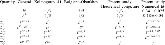
 $$\begin{eqnarray}{\mathcal{D}}_{\ell }\sim \ell ^{3h^{u}-1},\quad {\mathcal{D}}_{\ell }^{T}\sim \ell ^{h^{u}+2h^{T}-1},\quad {\mathcal{D}}_{\ell }^{c}\sim \ell ^{h^{u}+h^{T}},\quad {\mathcal{D}}_{\ell }^{\unicode[STIX]{x1D708}}\sim \ell ^{2h^{u}-2},\quad \text{and}\quad {\mathcal{D}}_{\ell }^{\unicode[STIX]{x1D705}}\sim \ell ^{2h^{T}-2}.\end{eqnarray}$$
In this framework, Kolmogorov scaling gives  $h^{u}=1/3$, and
 $h^{T}=1/3$. This should mean
 $$\begin{eqnarray}{\mathcal{D}}_{\ell }\sim \ell ^{0},\quad {\mathcal{D}}_{\ell }^{T}\sim \ell ^{0},\quad {\mathcal{D}}_{\ell }^{\unicode[STIX]{x1D708}}\sim \ell ^{-4/3},\quad {\mathcal{D}}_{\ell }^{\unicode[STIX]{x1D705}}\sim \ell ^{-4/3},\quad \text{and}\quad {\mathcal{D}}_{\ell }^{c}\sim \ell ^{2/3}.\end{eqnarray}$$
This regime is obtained when, in (3.9), the energy transfer is provided both by the thermal and the kinetic components:  ${\mathcal{D}}_{\ell }\sim \unicode[STIX]{x1D716},{\mathcal{D}}_{\ell }^{T}\sim \unicode[STIX]{x1D716}^{T}$.
Instead, in the Bolgiano–Oboukhov range, the energy transfer is provided by the thermal component, while the inertial term in the kinetic energy is affected by the exchange term. This corresponds to  ${\mathcal{D}}_{\ell }\sim {\mathcal{D}}_{\ell }^{c}$ and
 ${\mathcal{D}}_{\ell }^{T}\sim \unicode[STIX]{x1D716}_{T}$, resulting in
 $h^{u}=3/5$ and
 $h^{T}=1/5$, and therefore
 $$\begin{eqnarray}{\mathcal{D}}_{\ell }\sim \ell ^{-4/5},\quad {\mathcal{D}}_{\ell }^{T}\sim \ell ^{0},\quad {\mathcal{D}}_{\ell }^{\unicode[STIX]{x1D708}}\sim \ell ^{-4/5},\quad {\mathcal{D}}_{\ell }^{\unicode[STIX]{x1D705}}\sim \ell ^{-8/5},\quad \text{and}\quad {\mathcal{D}}_{\ell }^{c}\sim \ell ^{4/5}.\end{eqnarray}$$
Hence, by looking at the scaling properties of these quantities and at their balance, we can infer consistency with the Kolmogorov 41 or Bolgiano scaling. The scalings are summarized in table 2. It is worth emphasizing that these scalings are obtained through similarity arguments based on the locally isotropic hypothesis, so that deviations may be observed whenever this hypothesis is not fulfilled, notably for the coupling term.
An important empirical observations is that the standard deviation of the observables provides cleaner scaling laws (§ 4.4) than the average. We have not yet fully understood this issue, but the same trend has been found in independent experiments (Saw et al. Reference Saw, Kuzzay, Faranda, Guittonneau, Daviaud, Wiertel-Gasquet, Padilla and Dubrulle2016, Reference Saw, Debue, Kuzzay, Daviaud and Dubrulle2018). We think this is because fluctuations are more robust to changes in the orientation of the large-scale circulation of the flow than the time average. It is also possible that squared observables scale better because they are always positive, similarly to what is encountered in calculating structure functions (Benzi et al. Reference Benzi, Tripiccione, Massaioli, Succi and Ciliberto1994). We cannot however be assertive on this point, since we cannot use the absolute value in the filtering terms, and time averaging the absolute value of different quantities turns out to be rather inconclusive.
Summary of scaling laws for the different quantities appearing in equations (3.2) and (3.3), depending upon the scaling of velocity and temperature increments. The last two columns refer to the present study. The last one indicates the values extracted via a fit procedure of the data presented in § 4.4. We have used only  $Ra=10^{8}$ since the scaling range is larger. The exponents obtained by data at
 $Ra=10^{7}$ are however consistent with these values.

4 Results
4.1 Flow fields
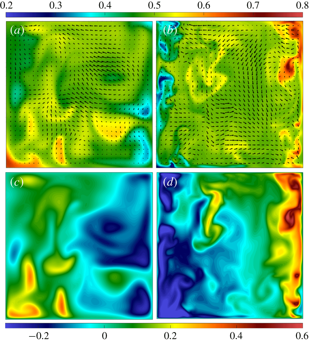
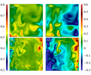
In figure 1 we show a horizontal slice of instantaneous temperature and velocity fields at the centre of the domain, the region we focus on in this work. It seems established that coherent thermal and velocity structures, the so-called thermal plumes, defined as a localized portion of fluid having a temperature contrast with the background, play a major role in the transport of heat in turbulent convection (Chillà & Schumacher Reference Chillà and Schumacher2012; Shang et al. Reference Shang, Qiu, Tong and Xia2003). These structures emerge from the dynamics of the boundary layer, and in the centre of the cell they are heavily impacted by the large-scale circulation (LSC), and the geometrical aspects of the flow may be quite different. Indeed, in figure 1 it is seen that cold plumes are directed mostly along one side of the cell while the hot plumes go up at the other side, because of the impingement of the fluid caused by LSC. These results are in line with experiments made in different geometries (Zhou, Sun & Xia Reference Zhou, Sun and Xia2007; Liot et al. Reference Liot, Seychelles, Zonta, Chibbaro, Coudarchet, Gasteuil, Pinton, Salort and Chillà2016).
(a,b) Instantaneous temperature and velocity fields in the horizontal  $x$–
 $y$ plane midway between the vertical walls. The velocity is superposed as vectors on the temperature map. The temperature colour bar is at the top of the figure. (c,d) Instantaneous heat fluxes, at the same instant of time and horizontal cross-section as the plots in (a,b). The heat flux colour bar is at the bottom of the figure. Results for different
 $Ra$ are displayed,
 $Ra=10^{7}$ in (a,c), and
 $Ra=10^{8}$ in (b,d).

4.2 Local Bolgiano–Oboukhov length scale
The correct reproduction of the large-scale dynamics together with the numerical assessment summarized in table 1 convincingly show that present simulations are fully resolved. Before going into the main subject of the present work, which is to use the weak formulation of the equations, it is useful to study the properties of  $L_{BO}$, which is an estimate of the distance at which the buoyancy and dissipative terms balance in the Boussinesq equations. It also represents the scale at which temperature cannot be considered passive anymore and therefore different scalings are expected. It is defined on a dimensional ground as
 $$\begin{eqnarray}\hat{L}_{BO}\equiv (\unicode[STIX]{x1D6FD}g)^{-3/2}\langle \hat{\unicode[STIX]{x1D716}}\rangle ^{5/4}\langle \hat{\unicode[STIX]{x1D716}_{T}}\rangle ^{-3/4},\end{eqnarray}$$
where we have used the hat  $\hat{~}$ symbol to highlight that the quantities in this formula are dimensional. A local version of this length can be defined in dimensionless form as
 $$\begin{eqnarray}L_{BO}^{local}(x,y,z)\equiv \langle \unicode[STIX]{x1D716}\rangle _{t}^{5/4}\langle \unicode[STIX]{x1D716}_{T}\rangle _{t}^{-3/4},\end{eqnarray}$$
where we use the non-dimensional dissipations. In this definition the length is obtained by averaging in time but not over the volume. It is known (Benzi et al. Reference Benzi, Toschi and Tripiccione1998; Calzavarini et al. Reference Calzavarini, Toschi and Tripiccione2002) that  $L_{BO}^{local}$ depends on the position in the convection cell and on the boundary conditions.
In particular, since we focus on the bulk region, we have computed the average
 $$\begin{eqnarray}L_{BO}^{bulk}=\langle \unicode[STIX]{x1D716}^{5/4}\rangle _{x,y,t}\langle \unicode[STIX]{x1D716}_{T}\rangle _{x,y,t}^{-3/4},\end{eqnarray}$$
calculated at  $z=0$, that is at the horizontal mid-plane at the centre of the cell. The average is made in time and over the bulk region defined as a square of side
 $0.8H$. This choice will be explained later in § 4.3. The value of
 $L_{BO}$ may also be roughly estimated using the
 $0$th law of turbulence and similar scaling for the temperature
 $\unicode[STIX]{x1D716}\sim u_{rms}^{3}/L$,
 $\unicode[STIX]{x1D716}_{T}\sim u_{rms}(\langle T^{\prime }\rangle )^{2}/L$, where we have considered a typical fluctuation of temperature
 $T^{\prime }$ and a typical length scale
 $L$ for velocity and temperature. Considering in the present case that these length scales are of the same order as the typical distance from the plates
 $z_{\ast }$, we get for a global length depending on the vertical coordinate:
 $\hat{L}_{BO}=(\unicode[STIX]{x1D6FD}g)^{-3/2}u_{rms}^{3}\langle T^{\prime }\rangle ^{-3/2}z_{\ast }^{-1/2}$.
It is seen from this expression that in the centre of the cell the estimate is  $\hat{L}_{BO}\sim H$, that is of the order of the cell dimension. The global averaged
 $L_{BO}$ turns out to be of the order of the entire height of the cube. In particular, we have found
 $L_{BO}^{bulk}\lesssim 0.5$ for both
 $Ra$. However, given that our problem is non-homogeneous with walls at the boundaries, the fluctuation statistics are also dependent on the distance from the sidewalls and thus this estimate does not permit us access to the local behaviour. We can only expect that, very near to the walls,
 $L_{BO}^{local}$ attains its maximum value. In particular, the local length formally diverges at the lateral walls because of the adiabatic conditions.
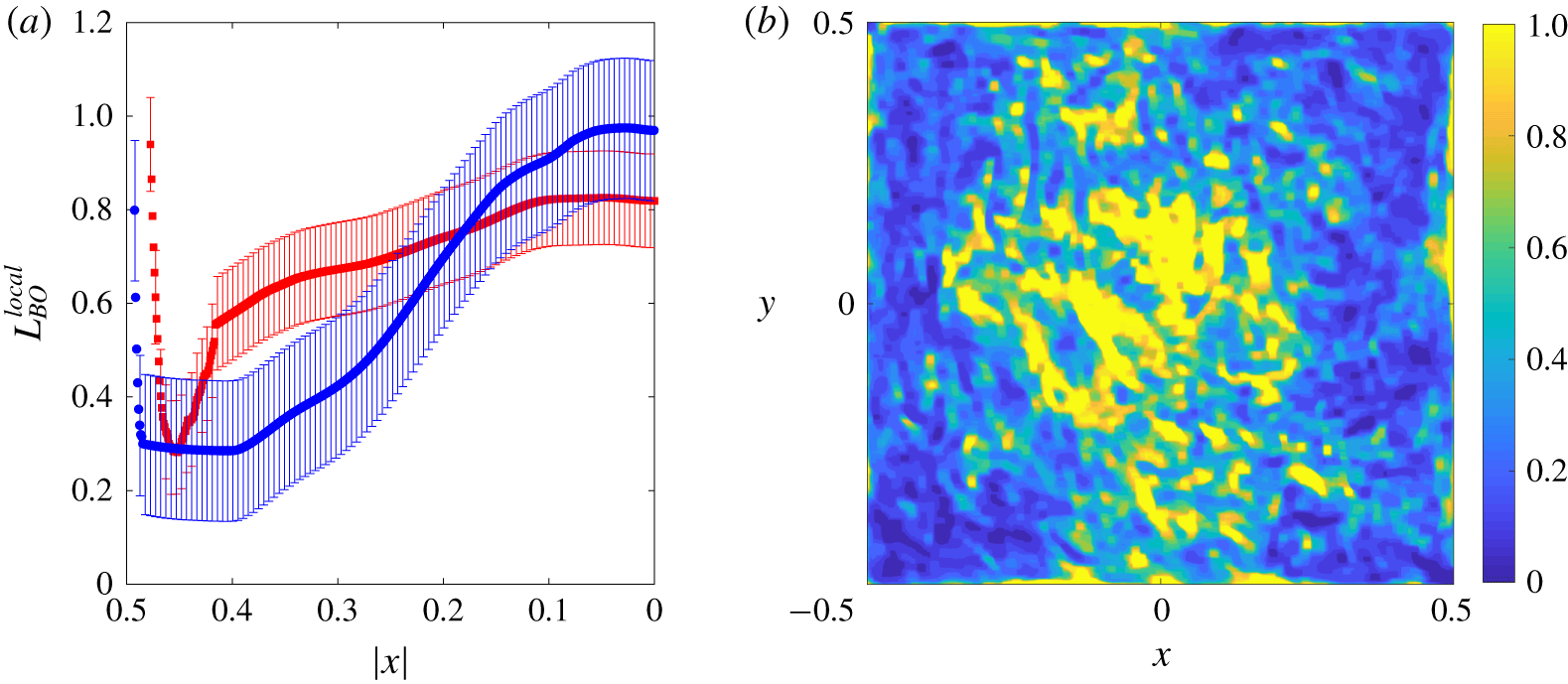
(a) Time-averaged profiles of the adimensional local Bolgiano–Oboukhov length scale ( $L_{BO}^{local}$) in the horizontal direction
 $(|x|)$, for
 $Ra=10^{7}$ (red squares) and
 $Ra=10^{8}$ (blue dots), with respective error bars. The error bars are twice the standard deviation of
 $L_{BO}^{local}$, which is globally estimated for all
 $x$ as the time and space average of the uncertainty of
 $L_{BO}^{local}$ at the centre of the cell (
 $|x|<0.2$), which is the region where
 $L_{BO}^{local}$ fluctuates the most. (b) Contour plot of the time-averaged adimensional
 $L_{BO}^{local}$ length scale on a horizontal section (
 $xy$) at half-height of the cell (
 $z=0$), at
 $Ra=10^{8}$.

To analyse this issue, in figure 2 the profiles of  $L_{BO}^{local}$ for the two
 $Ra$ numbers computed locally at the centre of the cube are shown. Both the entire horizontal plan and the length versus
 $x$ coordinate are reported.
Due to the symmetry of the flow, we only plot half of the profile along the  $x$ axis. It turns out that large variations of
 $L_{BO}^{local}$ are experienced through the entire region, more evidently for
 $Ra=10^{8}$. In particular, the length may be one order of magnitude shorter than the cell size locally, over a large span of the domain, at least for the higher
 $Ra$ case. This is highlighted in the map shown in figure 2(b). From the pictures, it should be noted that quantities averaged only in time are not perfectly at convergence and some fluctuations are always present. Our results are hence to be considered qualitative but not necessarily quantitative. The results are in any case very similar to those already presented in previous works (Benzi et al. Reference Benzi, Toschi and Tripiccione1998; Kaczorowski & Xia Reference Kaczorowski and Xia2013). Differences with respect to the more recent study appear within the statistical error bars, considering also that
 $Pr$ is slightly different, but it is known to have a huge impact. Moreover, since we use a much higher resolution, some small differences in the evaluation of dissipation can be expected. Globally, we can consider that these two works validate each other, since they use different numerical approaches. Residual differences with respect to the older work by Benzi et al. (Reference Benzi, Toschi and Tripiccione1998), are to be explained by the changes in boundary conditions. Our results therefore confirm also that the dynamics of the core region is significantly influenced by the boundary conditions. Moreover, present results confirm the possibility of finding a local BO scaling, separated from the Kolmogorov one, if local variations are properly computed.
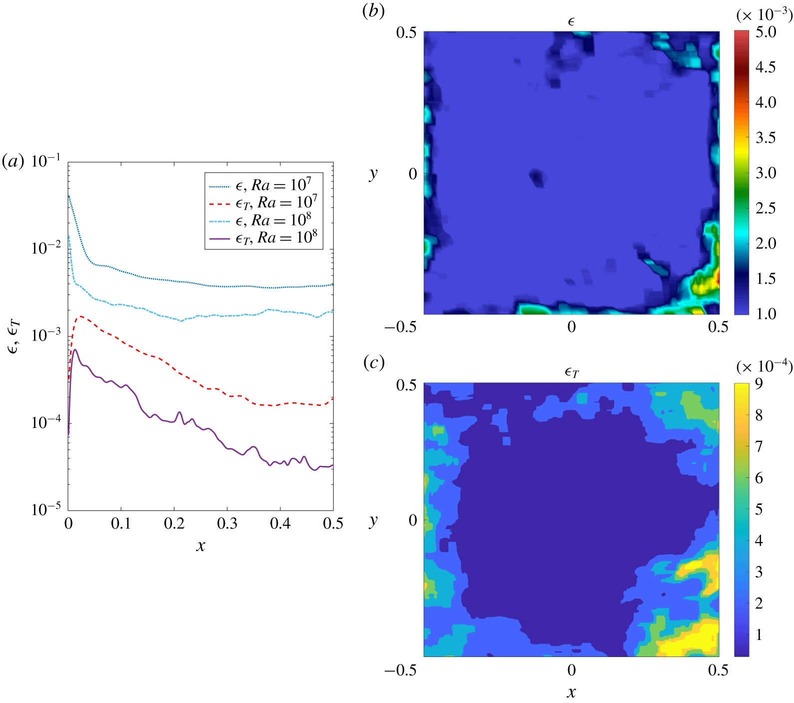
(a) Time-averaged profiles of the turbulent-kinetic-energy dissipation rate ( $\unicode[STIX]{x1D716}$) and temperature variance dissipation rate (
 $\unicode[STIX]{x1D716}_{T}$) in the horizontal direction (
 $x$). Continuous line:
 $\unicode[STIX]{x1D716}_{T}$, at
 $Ra=10^{8}$; dashed line:
 $\unicode[STIX]{x1D716}_{T}$, at
 $Ra=10^{7}$; dot-dashed line:
 $\unicode[STIX]{x1D716}$, at
 $Ra=10^{8}$; dotted line:
 $\unicode[STIX]{x1D716}$, at
 $Ra=10^{7}$. (b) Contour plot of the turbulent-kinetic-energy dissipation rate (
 $\unicode[STIX]{x1D716}$) values on a horizontal section (
 $xy$) at half-height of the cell (
 $z=0$). (c) Contour plot of the temperature variance dissipation rate (
 $\unicode[STIX]{x1D716}_{T}$) values on a horizontal section (
 $xy$) at half-height of the cell (
 $z=0$).

Since in the definition of  $L_{BO}$ the energy and thermal variance dissipation are used, we show in figure 3 the profiles of those functions, figure 3(a), together with the surface contour for the
 $Ra=10^{8}$ case. Once again, profiles obtained are similar to those shown in recent computations carried out in an analogous configuration (Kaczorowski & Xia Reference Kaczorowski and Xia2013). The profiles obtained at two different
 $Ra$ numbers elucidate how
 $L_{BO}$ depends on the forcing parameter. It should be clear also from these results that the direct measurement of this length based on its definition (4.1), is particularly delicate, because it is based on the ratio of powers of the statistics of very small-scale observables, which wildly fluctuate. Furthermore, it should be emphasized that the definition (4.1) is physically sound but does not consider the characteristics of the flow, so that a pre-factor (possibly non-universal) should be present, and there is no reason to be sure that this pre-factor is of order one (Monin & Yaglom Reference Monin and Yaglom1975). In the following section we shall estimate
 $L_{BO}$ looking at the scaling laws and we will compare the results. Specifically, we will seek the scale at which a cross-over in the scaling is encountered because of buoyancy.
4.3 Wavelet analysis
Energy balances are computed on the horizontal section at half-height of the Rayleigh–Bénard cell. In this section, all the three components of the velocity field, and its derivatives in two dimensions, are taken into account. Balances for a wide range of scales  $\ell$ are calculated by using a Gaussian filtering function
 $G_{\ell }(\boldsymbol{r})\sim e^{-|\boldsymbol{r}|^{2}/2}$, where
 $\boldsymbol{r}=\boldsymbol{x}/\ell$ is a scale-dependent spatial coordinate.
In equations (4.4)–(4.8), the terms of the filtered kinetic and thermal energy balances defined in (3.2) and (3.3) are written explicitly as a function of the instantaneous velocity ( $\boldsymbol{u}$) and temperature (
 $\unicode[STIX]{x1D703}$) fields.
 $$\begin{eqnarray}\displaystyle & \displaystyle \text{D}_{\ell }=\frac{1}{4}\int d^{d}r(\unicode[STIX]{x1D735}G_{\ell }(\boldsymbol{r}))\boldsymbol{\cdot }[\boldsymbol{u}(\boldsymbol{x}+\boldsymbol{r},t)-\boldsymbol{u}(\boldsymbol{x},t)][\boldsymbol{u}(\boldsymbol{x}+\boldsymbol{r},t)-\boldsymbol{u}(\boldsymbol{x},t)]^{2}, & \displaystyle\end{eqnarray}$$
 $$\begin{eqnarray}\displaystyle & \displaystyle \text{D}_{\ell }^{T}=\frac{1}{4}\int d^{d}r(\unicode[STIX]{x1D735}G_{\ell }(\boldsymbol{r}))\boldsymbol{\cdot }[\boldsymbol{u}(\boldsymbol{x}+\boldsymbol{r},t)-\boldsymbol{u}(\boldsymbol{x},t)][\unicode[STIX]{x1D703}(\boldsymbol{x}+\boldsymbol{r},t)-\unicode[STIX]{x1D703}(\boldsymbol{x},t)]^{2}, & \displaystyle\end{eqnarray}$$
 $$\begin{eqnarray}\displaystyle & \displaystyle \text{D}_{\ell }^{\unicode[STIX]{x1D708}}=\frac{1}{\sqrt{RaPr}}\int d^{d}r(\unicode[STIX]{x1D6FB}^{2}G_{\ell }(\boldsymbol{r}))\left[\boldsymbol{u}(\boldsymbol{x}+\boldsymbol{r},t)\boldsymbol{\cdot }\boldsymbol{u}(\boldsymbol{x},t)-\frac{\boldsymbol{u}(\boldsymbol{x}+\boldsymbol{r},t)\boldsymbol{\cdot }\boldsymbol{u}(\boldsymbol{x}+\boldsymbol{r},t)}{2}\right], & \displaystyle\end{eqnarray}$$
 $$\begin{eqnarray}\displaystyle & \displaystyle \text{D}_{\ell }^{\unicode[STIX]{x1D705}}=\frac{1}{\sqrt{RaPr}}\int d^{d}r(\unicode[STIX]{x1D6FB}^{2}G_{\ell }(\boldsymbol{r}))\left[\unicode[STIX]{x1D703}(\boldsymbol{x}+\boldsymbol{r},t)\cdot \unicode[STIX]{x1D703}(\boldsymbol{x},t)-\frac{\unicode[STIX]{x1D703}^{2}(\boldsymbol{x}+\boldsymbol{r},t)}{2}\right], & \displaystyle\end{eqnarray}$$
 $$\begin{eqnarray}\displaystyle & \displaystyle \text{D}_{\ell }^{c}=\frac{1}{2}\left[\boldsymbol{u}(\boldsymbol{r},t)\boldsymbol{\cdot }\frac{\boldsymbol{g}}{|\boldsymbol{g}|}\int d^{d}r(G_{\ell }(\boldsymbol{r}))\unicode[STIX]{x1D703}(\boldsymbol{x}+\boldsymbol{r},t)+\unicode[STIX]{x1D703}(\boldsymbol{r},t)\int d^{d}r(G_{\ell }(\boldsymbol{r}))\boldsymbol{u}(\boldsymbol{x}+\boldsymbol{r},t)\boldsymbol{\cdot }\frac{\boldsymbol{g}}{|\boldsymbol{g}|}\right]. & \displaystyle \nonumber\\ \displaystyle & & \displaystyle\end{eqnarray}$$
The convolution integrals in equations (4.4), (4.5), (4.6), (4.7) and (4.8) can be computed efficiently using continuous wavelets transforms, based on fast Fourier transforms. In this study, we use the two-dimensional continuous wavelet MATLAB package provided by the toolbox YAWTB (http://sites.uclouvain.be/ispgroup/yawtb).
The terms  $\text{D}_{\ell }$,
 $\text{D}_{\ell }^{T}$,
 $\text{D}_{\ell }^{\unicode[STIX]{x1D708}}$,
 $\text{D}_{\ell }^{\unicode[STIX]{x1D705}}$ and
 $\text{D}_{\ell }^{c}$ are averaged over the time duration of each simulation (after reaching statistically steady conditions), and space over the region of the cell investigated, to get
 ${\mathcal{D}}_{\ell }$,
 ${\mathcal{D}}_{\ell }^{T}$,
 ${\mathcal{D}}_{\ell }^{\unicode[STIX]{x1D708}}$,
 ${\mathcal{D}}_{\ell }^{\unicode[STIX]{x1D705}}$ and
 ${\mathcal{D}}_{\ell }^{c}$. In particular, approximately
 $900$ independent snapshots of the flow have been used. The snapshots have been collected over a simulation of approximately 300 reference time durations (in the steady state). Statistical convergence of the budgets has been checked verifying that the results are basically unchanged using half of the data.
Concerning the spatial regions analysed in this work, we have studied the energy budgets in two regions of the plane at  $z=0$. The bulk region is chosen by excluding 100 data points from each sidewall, that is approximately 4 times the boundary-layer thickness
 $\unicode[STIX]{x1D6FF}_{\unicode[STIX]{x1D703}}$ for the case at
 $Ra=10^{7}$, and approximately
 $7\unicode[STIX]{x1D6FF}_{\unicode[STIX]{x1D703}}$ for
 $Ra=10^{8}$. In wavelet analysis on non-periodic flows, it is necessary to eliminate a border region to avoid spurious effects, and this choice of the bulk turns out to minimize the effects of the boundaries on the computation of the convolution integrals (4.4)–(4.8). We have checked that equivalent results are obtained with a different choice of the bulk region (from
 $0.6H$ to
 $0.9H$. The second region analysed is the region adjacent to the sidewall. We have chosen the region which extends from the sidewall
 $8\unicode[STIX]{x1D6FF}_{\unicode[STIX]{x1D703}}$ for the case at
 $Ra=10^{7}$, and approximately
 $15\unicode[STIX]{x1D6FF}_{\unicode[STIX]{x1D703}}$ for
 $Ra=10^{8}$. We have checked that results are barely modified by taking a little larger or smaller region.
4.4 Scaling laws
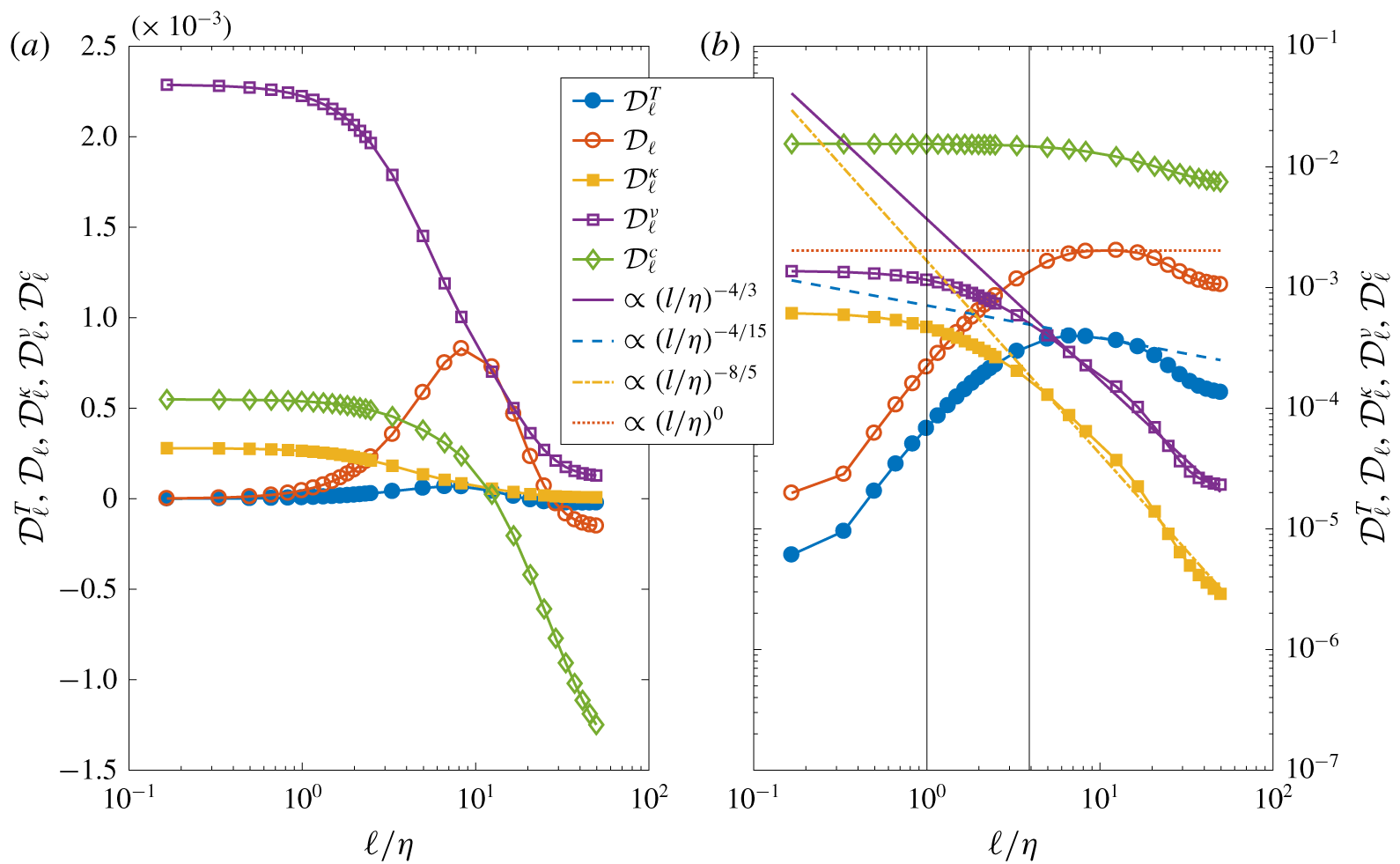
Time- and space-averaged energy balance terms (a), and their time-averaged spatial standard deviations (b), as a function of scale  $\ell$ over the Kolmogorov length scale
 $\unicode[STIX]{x1D702}$, in the bulk region for
 $Ra=10^{7}$. Spatial averages and standard deviations were computed in the bulk region, on a horizontal slice at half-height of the cell. The terms of the energy balance at scale
 $\ell$ are:
 ${\mathcal{D}}_{\ell }^{T}$: thermal energy term;
 ${\mathcal{D}}_{\ell }$: kinetic energy transfer term;
 ${\mathcal{D}}_{\ell }^{\unicode[STIX]{x1D705}}$: thermal dissipation term;
 ${\mathcal{D}}_{\ell }^{\unicode[STIX]{x1D708}}$: viscous dissipation term;
 ${\mathcal{D}}_{\ell }^{c}$: exchange term between kinetic and thermal energy; the two vertical black lines correspond to the Kolmogorov scale,
 $\unicode[STIX]{x1D702}$, and to the scale where the Bolgiano–Oboukhov regime becomes visible in the scalings.

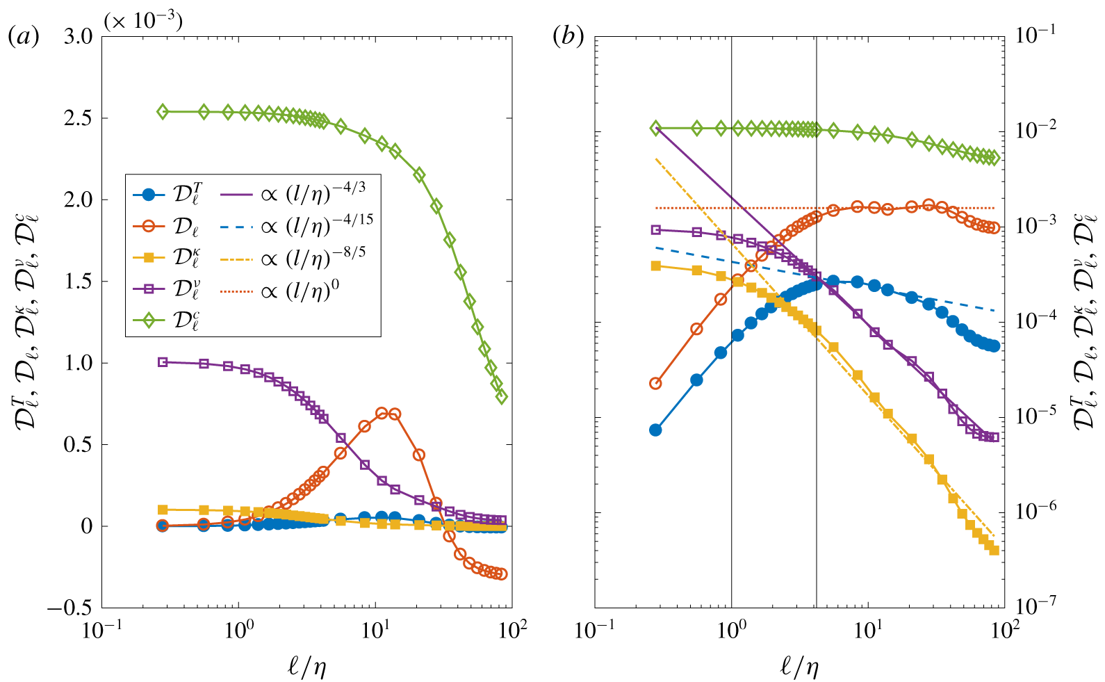
In figures 4–5, we show the main results of the present work, that is the scaling behaviour of the mean and standard deviations of all terms of equations (3.2)–(3.3) once averaged over space and time for both  $Ra$ numbers.
Comparing figure 4(a) with 5(a), we see that the balance of terms depends strongly upon the Rayleigh number: at  $Ra=10^{7}$, the viscous terms
 ${\mathcal{D}}_{\ell }^{\unicode[STIX]{x1D708}}$ is the largest at all scales, indicating that we are mainly in a dissipative regime. There is a small inertial interval around
 $\ell /\unicode[STIX]{x1D702}=10$, where the kinetic energy transfer term
 ${\mathcal{D}}_{\ell }$ and the thermal energy term
 ${\mathcal{D}}_{\ell }^{T}$ peak, indicating non-trivial turbulent behaviour. Indeed, the standard deviation (right panel) displays small inertial scaling range at this location. Moreover, the buoyancy term start being appreciable at
 $\ell \approx 5\unicode[STIX]{x1D702}$ and becomes dominant at
 $\ell \approx 20\unicode[STIX]{x1D702}$. In contrast, for
 $Ra=10^{8}$, the viscous term is dominant only up to
 $\ell \approx 5\unicode[STIX]{x1D702}$, and the coupling term
 ${\mathcal{D}}_{\ell }^{c}$ becomes dominant for
 $\ell \approx 25\unicode[STIX]{x1D702}$, indicating a strongly convective regime. The kinetic energy transfer term
 ${\mathcal{D}}_{\ell }$ and the thermal energy term
 ${\mathcal{D}}_{\ell }^{T}$ still peak around
 $\ell /\unicode[STIX]{x1D702}=10$, with a wider inertial scaling range for the standard deviation. Still concerning the exchange term, it is worth noting that, at scales between the dissipative scale and the integral one, this term may be negative. This is found to be particularly true in the regions not far from the walls. However, it should be noted that the scaling analysis of the exchange term
 ${\mathcal{D}}_{\ell }^{c}$ is rather inconclusive with the present data, indicating that boundary effects are important.
Time- and space-averaged energy balance terms (a), and their time-averaged spatial standard deviations (b), as a function of scale  $\ell$ over the Kolmogorov length scale
 $\unicode[STIX]{x1D702}$, for
 $Ra=10^{8}$. See figure 4 for spatial averaging details, and description of legend terms.

As anticipated, the standard deviations of the observables display a much cleaner scaling than the mean quantities. We thus focus on them for the discussion of the scaling shape. Looking at the scaling of fluctuations figures 4(b)–5(b), the dynamics appears qualitatively quasi-independent of  $Ra$ number, at least in the present range, at variance with the scalings provided by the global averages. In practice, scalings at
 $Ra=10^{8}$ are clearer because of the smaller finite-
 $Re$ effect in this more turbulent regime. A qualitative picture could however also be inferred from the lower
 $Ra$ number. In any case, to be sure to limit the viscous effect, we concentrate on the behaviour at
 $Ra=10^{8}$ in the following.
In the range  $5\unicode[STIX]{x1D702}\lesssim \ell \lesssim 30\unicode[STIX]{x1D702}$, the buoyancy term is found to be greater than the nonlinear thermal transfer but smaller than the kinetic energy one. This means that
 $L_{BO}$ can be physically estimated as
 $L_{BO}\sim 5\div 10\unicode[STIX]{x1D702}$, and that, starting from this point, Bolgiano scalings may be expected. This empirical estimate differs therefore from that obtained using the global definition (4.2).
In this range, the thermal dissipation term is consistent with  ${\mathcal{D}}^{\unicode[STIX]{x1D705}}\sim \ell ^{-8/5}$, while the viscous one scales like
 ${\mathcal{D}}_{\unicode[STIX]{x1D708}}\sim \ell ^{-4/3}$. In both cases, the scaling appears to be robust and extends over approximately one decade. Therefore, it turns out that in this range a Kolmogorov inertial scaling for the velocity but a BO scaling for the temperature are found. Finally, the nonlinear transfer term of the temperature equation is well reproduced by
 ${\mathcal{D}}^{T}\sim \ell ^{-4/15}$. Below
 $L_{BO}$, for
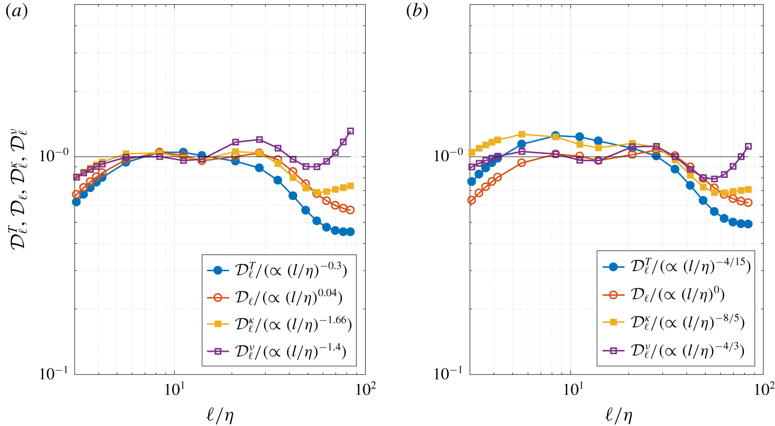
 $\ell \lesssim 5\unicode[STIX]{x1D702}$ scalings change clearly for all observables, but it is hard to extract the slope. As a conjecture we have used the typical exponents related to similarity analysis and the related curves are displayed in figures 4(b)–5(b). To corroborate the picture, we have extracted the scaling exponents via the fitting of our data, and they are presented in table 1 with the corresponding error for
 $Ra=10^{8}$. We present also in figure 6 the compensated plots both for the best fitting exponents and the conjectured ones. It is seen that the numerical exponents are all consistent with the similarity ones, which will be therefore used for the following discussion.
(a) Compensated plots of the budgets terms and the best fitting curves. (b) Compensated plots of the budgets terms and the conjectured scaling exponents related to similarity analysis.

We can now analyse the scalings found from figure 5 in terms of scaling exponents within the general Kolmogorov–Onsager framework presented in § 3.4. From  $\ell \gtrapprox 4\unicode[STIX]{x1D702}$ a Bolgiano scaling is found for
 ${\mathcal{D}}_{\ell }^{\unicode[STIX]{x1D705}}$, so that
 $h^{T}=1/5$. This is in line with the previous empirical estimate of
 $L_{BO}\sim 5\unicode[STIX]{x1D702}$, where we observed that the exchange term becomes more important than the thermal transfer term. However, in the range
 $\unicode[STIX]{x1D702}<\ell \lesssim 30\unicode[STIX]{x1D702}$, the velocity observables follow a Kolmogorov-like scaling with
 ${\mathcal{D}}_{\ell }\sim \ell ^{0},{\mathcal{D}}_{\ell }^{\unicode[STIX]{x1D708}}\sim \ell ^{-4/3}$, such that
 $h^{u}=1/3$. Consistently,
 ${\mathcal{D}}_{\ell }^{T}\sim \ell ^{h^{u}+2h^{T}-1}=\ell ^{-4/15}$, as displayed in figure 5 for
 $\ell \gtrapprox 5\div 10\unicode[STIX]{x1D702}$. Hence, in this range, the buoyancy term remains smaller than the nonlinear inertial term of kinetic energy and a Kolmogorov scaling is observed for the velocity. In the range
 $\ell >30\unicode[STIX]{x1D702}$, the buoyancy effects are dominant with respect to all other terms, and a pure Bolgiano–Oboukhov scaling should be present. Boundary effects and the lack of a sufficient number of scales make this conjecture speculative for the moment. In the discussion section we suggest that anisotropy is responsible for the mixed scaling we obtain. On the other hand, in the range
 $\ell <L_{BO}\approx 5\unicode[STIX]{x1D702}$, all the scalings might be consistent with the Kolmogorov picture, even though we can only analyse a very small range of scales. In particular,
 ${\mathcal{D}}_{\ell }^{T}\sim \ell ^{0}$, and
 ${\mathcal{D}}_{\ell }^{\unicode[STIX]{x1D705}}\sim \ell ^{-4/3}$.
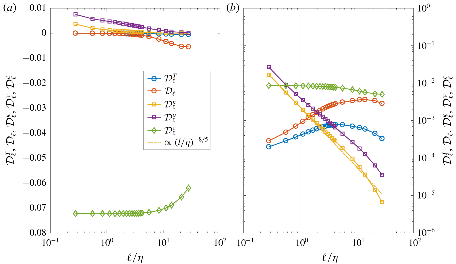
Time- and space-averaged energy balance terms (a) and their time-averaged spatial standard deviations (b), as a function of scale  $\ell$ over the Kolmogorov length scale
 $\unicode[STIX]{x1D702}$, for
 $Ra=10^{8}$. Spatial averages and standard deviations were computed in the boundary-layer region, on a horizontal slice at half-height of the cube. The terms of the energy balance at scale
 $\ell$ are:
 ${\mathcal{D}}_{\ell }^{T}$: thermal energy term;
 ${\mathcal{D}}_{\ell }$: kinetic energy transfer term;
 ${\mathcal{D}}_{\ell }^{\unicode[STIX]{x1D705}}$: thermal dissipation term;
 ${\mathcal{D}}_{\ell }^{\unicode[STIX]{x1D708}}$: viscous dissipation term;
 ${\mathcal{D}}_{\ell }^{c}$: exchange term between kinetic and thermal energy; the vertical black line corresponds to the Kolmogorov scale,
 $\unicode[STIX]{x1D702}$.

It is interesting to look also at statistics in the region near to the walls, that is in the boundary layer. Indeed, as displayed in figure 2, we expect that  $L_{BO}^{local}$ has a minimum in the boundary-layer region very close to the walls, and therefore buoyancy effects should start to be dominant even at a smaller scale. Yet, it is important to note here that, with respect to the results obtained in the bulk region, the boundary-layer statistics should be handled with much care and in no case considered as conclusive, for several reasons. To get these statistics we consider approximately
 $15\unicode[STIX]{x1D6FF}_{\unicode[STIX]{x1D703}}$, which means only the first
 $200$ points near to each boundary, so that the number of scales available is small and no clear scale separation can be expected. Furthermore, these regions are strongly non-homogeneous and impacted by viscous effects, inducing without any doubt spurious effects on the statistics, so that the significance of the results must not be considered certain. In figure 7, we show the results obtained for the different observables at
 $Ra=10^{8}$. Even with the caveat about the applicability of the theory near the boundaries, the results are interesting. In this region a BO scaling seems to be found for both temperature and velocity in the range
 $\unicode[STIX]{x1D702}\lesssim \ell \lesssim 10\unicode[STIX]{x1D702}$, in particular scalings are consistent with
 ${\mathcal{D}}_{\ell }\sim \ell ^{4/5},{\mathcal{D}}_{\ell }^{T}\sim \ell ^{0},{\mathcal{D}}_{\ell }^{\unicode[STIX]{x1D705}}\sim \ell ^{-8/5}$. Yet the viscous term appears to have a scaling
 ${\mathcal{D}}_{\unicode[STIX]{x1D708}}\sim \ell ^{-1}$. It is therefore a little steeper than what is expected in the BO range. These findings confirm the importance of local properties of the fields and the necessity of accurately disentangling them from more global effects. Since near the boundaries
 $L_{BO}$ becomes small, the BO scalings are more effective for both velocity and temperature. The slightly inconsistent behaviour of the velocity dissipation term is thought to be related to finite
 $Re$ effects, since near the boundaries the local
 $Re$ number is not large and the similarity arguments à la Kolmogorov are not expected to hold.
5 Discussion and conclusions
We have carried out a very highly resolved DNS analysis of the small-scale properties of turbulent Rayleigh–Bénard convection in a cubic cell at  $Pr=1$. The unusually accurate resolution allows us to go well below the Kolmogorov length. We have used two simulations at
 $Ra=10^{7}$ and
 $Ra=10^{8}$. It has long been known that there is a transition between a chaotic to a fully developed state around these values of
 $Ra$ (Siggia Reference Siggia1994). Although it is now widely accepted that the transition is not sharp as initially guessed (Castaing et al. Reference Castaing, Gunaratne, Heslot, Kadanoff, Libchaber, Thomae, Wu, Zaleski and Zanetti1989) it is interesting to capture possible signatures of a transition in scaling laws. Our main goal was to apply a new approach based on the weak formulation of the mathematical problem, and to extract in this way scaling exponents.
Previous experiments and numerical simulations have shown that BO scaling should be easier to observe at higher  $Pr$ number (Kaczorowski & Xia Reference Kaczorowski and Xia2013). However, the dependence on the
 $Pr$ number turned out to be moderate, and given that we need a very high resolution to properly compute local scaling at small scales, numerical simulations respecting the level of accuracy we have required in the present work would be unfeasible. Considering also that our main goal here was to show how new insights may come from the weak approach to turbulent problems, this explains why we have simulated a flow with
 $Pr=1$. The question of investigating some local properties at higher
 $Pr$ remains nevertheless relevant in many respects. As already indicated in previous numerical works, we have found that
 $L_{BO}^{local}$ is a strongly varying function of the position, on a horizontal cross-section of the domain, with the maximum at the vertical walls and a minimum approximately at the end of the boundary layer. The complex behaviour of the length is due to its dependence on the thermal and kinetic dissipation. The global
 $L_{BO}$ is found more or less the same for the two
 $Ra$ and of the order of the fluid layer height. Globally speaking, the results concerning the observable statistics of the flow are in good agreement with previous results. Since our simulations have been conducted with a different method than in the other studies, this is an indication of robustness that corroborates the findings. From the theoretical point of view, we have presented the derivation of the weak formulation or coarse-grained version of the Boussinesq equations for turbulent convection, which allows a smoothed treatment of instantaneous fluctuations. The resulting set of equations have been averaged in the present work to get the generalization of the Kármán–Howarth–Monin and Yaglom equation for the fully non-homogeneous problem. In our geometry, these equations are analogous to those obtained in recent work directly from the Boussinesq equations (Rincon Reference Rincon2006) and permit a clear scale-by-scale analysis of the turbulence cascade in the physical space. This original approach is useful to obtain scaling behaviour in a less noisy manner with respect to more standard statistical procedures. Moreover, when applied to the fluctuating equations, it allows us to get information on the probability distribution of fluxes, which is crucial to characterize extreme events and intermittency. Therefore, the approach presented in this work should be valuable to get new insights also in convective turbulence.
Using this filtering approach, we have analysed the scalings characterizing the kinetic energy and temperature variance cascade on a horizontal cross-section of the domain. The different scalings we found are reported in table 2. We have not found evidence of a standard BO scaling, which would mean  $h_{u}=3/5,h_{T}=1/5$. Instead, our numerical experiment points out that only the temperature follows this BO scaling, so that buoyancy effects are found to be dominant on the temperature variance budget at small scales. Yet the velocity follows the Kolmogorov 41 scaling
 $h_{u}=1/3$, at least in the available range of scales.
Such peculiar behaviour can be explained by removing the isotropic condition, and consider that the horizontal velocity increments and the vertical velocity increment scale with a different exponent, respectively  $h_{u}^{H}$ and
 $h_{u}^{V}$. In such a case, it is easy to see that the scaling exponents
 ${\mathcal{D}}$,
 ${\mathcal{D}}^{T}$,
 ${\mathcal{D}}^{\unicode[STIX]{x1D708}}$,
 ${\mathcal{D}}^{\unicode[STIX]{x1D705}}$ will be respectively
 $\min (3h_{u}^{H}-1,3h_{u}^{V}-1)$,
 $\min (h_{u}^{H}+2h_{T},h_{u}^{V}+2h_{T})$,
 $\min (2h_{u}^{H}-2,2h_{u}^{V}-2)$,
 $2h_{T}-2$. If we take
 $h_{u}^{H}=1/3$,
 $h_{u}^{V}=3/5$ and
 $h_{T}=1/5$, we thus get the theoretical results of table 2.
Moreover, the present results are compatible with the previous studies by Kunnen et al. (Reference Kunnen, Clercx, Geurts, van Bokhoven, Akkermans and Verzicco2008), Kaczorowski & Xia (Reference Kaczorowski and Xia2013). Although the scalings were extracted on very few points, temperature structure functions indicated a BO scaling whereas the velocity structure functions were less well defined. More importantly, only the axial functions showed some hint of BO scaling, while the horizontal ones had no conclusive scaling. That points to a possible anisotropic effect which may affect only velocity. Moreover, in the numerical study by Camussi & Verzicco (Reference Camussi and Verzicco2004) a BO scaling for the temperature and a Kolmorgorov 41 for the velocity were also found. In experiments, while evidence of BO scaling on the temperature has been available for some time (Wu et al. Reference Wu, Kadanoff, Libchaber and Sano1990; Cioni et al. Reference Cioni, Ciliberto and Sommeria1995; Ashkenazi & Steinberg Reference Ashkenazi and Steinberg1999), velocity scaling is more elusive and the effect of anisotropy has been also reported (Ching et al. Reference Ching, Chui, Shang, Qiu, Tong and Xia2004; Sun, Zhou & Xia Reference Sun, Zhou and Xia2006; Ching Reference Ching2007).
Then, the presence of lateral walls is found to be key in the possible change of scaling in the core of the flow. Indeed, because of walls: (a)  $L_{BO}^{local}$ experiences large variability and notably may be ten times less than the global one that is of the order of the cell length. This explains why, in horizontal homogeneous simulations, the BO range should not be observed at least in the core of the flow (Lohse & Xia Reference Lohse and Xia2010; Verma, Kumar & Pandey Reference Verma, Kumar and Pandey2017). (b) Since the flow is non-homogeneous, the budget equation for kinetic energy and temperature variance are complex, and transport terms play locally a role, as recently emphasized in a scale-by-scale analysis using another approach (Togni et al. Reference Togni, Cimarelli and De Angelis2015). In particular, it is found that, at variance with the homogeneous case, the coupling term may be locally negative at small scales, and in particular in the vicinity of the boundary layer, so that kinetic energy is converted to potential energy. Our numerical evidence hence confirms a previous theoretical analysis (Lvov Reference Lvov1991; L’vov & Falkovich Reference L’vov and Falkovich1992). Instead, in the homogeneous case the contrary has been found, which may lead to the impossibility of observing a BO scaling (Verma et al. Reference Verma, Kumar and Pandey2017). (c) The contribution of the buoyancy coupling term is found to be important at all scales, as reported previously (Togni et al. Reference Togni, Cimarelli and De Angelis2015), however, its relative importance with respect to other terms differs. Notably, it is found to be dominant in the temperature budget at almost all scales, whereas the inertial term of the kinetic energy budget is the most important term at small scales.
From the above considerations, we can draw the following picture: the presence of vertical walls makes  $L_{BO}^{local}$ small, and buoyancy is effective in the budget of temperature variance over a wide range of scales. That allows the emergence of a BO scaling on the temperature and on the vertical velocity component in the whole core region. On the other hand, in the bulk region, the nonlinear inertial term remains much greater than the buoyancy one and starts decreasing only at scales too large to allow the identification of a possible BO scaling for the horizontal velocity components, hence the Kolmorgorov 41 scaling is observed. In the vertical boundary-layer region,
 $L_{BO}^{local}$ may be much smaller than the global one and the non-homogeneous character of the region makes the redistribution among velocity components important. The local approach used here indicates indeed a possible BO scaling for the temperature and velocity, but some discrepancy in the viscous term that is attributed to a finite
 $Re$ correction. It is worth emphasizing, however, that the small number of points available in the vertical boundary layer and the difficulties inherent to such a non-homogeneous region make our reasoning not at all definitive, and begs a deeper analysis of the issue. In particular, the scaling of the velocity in this region is also compatible with
 $h_{u}=2/3$, which is typical of shear flows (Biferale & Procaccia Reference Biferale and Procaccia2005).
As far as it concerns the effect of Rayleigh number, comparing two set of results obtained at different  $Ra$, we have also shown that some differences are related to the transition from a chaotic (
 $Ra=10^{7}$) to a more turbulent regime (
 $Ra=10^{8}$). In particular, the viscous terms in the energy and temperature budgets are important at all scales at
 $Ra=10^{7}$, and not only in the vertical boundary layer. This indicates that much of the transport is always due to viscous diffusion, whereas it becomes negligible at
 $Ra=10^{8}$ at least in the core of the flow.
In the present paper, we have focused only on average quantities, performing the average over selected portions of the domains. The interest of our formulation, however, is that it also provides an expression for the local transfer quantities. It would be interesting to connect those local energy transfer to possible intermittency of the convective fluids. We leave that for future work.
Acknowledgements
We thank the anonymous reviewers for the careful reading of the first version of the manuscript, and for having pointed out many interesting remarks. This work has been supported by the ANR EXPLOIT, grant agreement no. ANR-16-CE06-0006-01. We acknowledge PRACE for awarding us access to Marconi at CINECA, Italy under the grant no. 2018184426.