


In the United States, it is not only corrupt conduct by elected officials, but also its detection and prosecution that may have significant political consequences. On the one hand, officials may undertake illegal activities to further their political fortunes. For example, an incumbent might seek to further his or her political career by accepting a bribe, rigging a competitive bidding process to secure the support of an influential private citizen, or diverting public resources into his or her reelection campaign. At the same time, the prosecution of corrupt practices—whether real or merely alleged—can also produce political fallout. An investigation or indictment can irreversibly harm the future career prospects of the official under scrutiny, even if that individual is eventually exonerated.
Discretion over whether to bring forward a criminal case lies largely with the prosecutor.Footnote 1 In the enforcement of federal public corruption laws, this authority rests almost entirely in the hands of U.S. Attorneys in the Department of Justice (DOJ). U.S. Attorneys are political appointees, raising the possibility that this discretion might be deployed in public corruption cases on the basis of partisan political motivations. If U.S. Attorneys are motivated to embarrass or discredit political opponents through an indictment, they might decide to bring relatively weak cases they would otherwise decline. Alternatively, those officials might decline to prosecute co-partisans except in the most egregious cases. On the other hand, federal prosecutors might be limited in the degree to which they can act on partisan motivations even to the extent that they harbor them, whether by formal institutional constraints or by informal norms of professional ethical conduct.
The issue of partisan bias in federal corruption prosecutions became the subject of public attention in 2007, when newly empowered Democratic congressional majorities convened hearings to investigate the dismissal of a number of U.S. Attorneys by the administration of George W. Bush in the previous two years. Critics have contended that some of these officials may have been dismissed either because they did not pursue corruption investigations against prominent Democrats with sufficient vigor or because they did pursue investigations against prominent Republicans (Goldstein and Eggen Reference Goldstein and Eggen2007; Lipton Reference Lipton2007a). Others have pointed to high-profile prosecutions of Democrats, such as Alabama Governor Donald Siegelman, as evidence of politicized prosecution (Lipton Reference Lipton2007b).
Moving beyond these high-profile cases, have Bush-appointed U.S. Attorneys systematically targeted Democratic public officials or avoided targeting Republicans for public corruption prosecutions? To the extent that partisan motivations have influenced such prosecutions, has the phenomenon been unique to the Bush administration? This article proposes an approach to address these questions systematically. First, I evaluate the conclusions of a recent, widely cited study suggesting that Democrats were up to seven times more likely to be investigated by the Bush Justice Department than were Republicans (Shields and Cragan Reference Shields and Cragan2007). I argue that our ability to infer partisan bias by the Justice Department from the study's data on publicized investigations is sharply limited. Because U.S. Attorneys nearly always prosecute cases that have been referred by other investigative agencies such as the Federal Bureau of Investigation (FBI) or state and local law enforcement, the absence of information (owing to privacy concerns) on the partisan breakdown of referrals not taken up by prosecutors threatens to invalidate the authors' claims of selective prosecution.
Second, I develop a simple model of prosecutorial discretion in the presence of (possible) partisan bias. Employing an approach from economic models of discrimination, I treat partisan bias as a “taste” or preference for prosecuting one's political opponents (or for not prosecuting allies). This approach, pioneered by Becker (Reference Becker1957), has been employed recently to study discrimination against minorities in setting bail (Ayres Reference Ayres2001; Ayres and Waldfogel Reference Ayres and Waldfogel1994), racial profiling (Knowles, Persico, and Todd Reference Knowles, Persico and Todd2001), and discrimination against female candidates in congressional elections (Anzia and Berry Reference Anzia and Berry2007). In the model, the prosecutor receives a signal of the official's culpability (the referral) and decides whether to pursue the case. A biased prosecutor's relative enthusiasm for pursuing cases against political opponents will lead her to prosecute weaker cases than she would against her allies. The empirical implication of this behavioral effect is that in the presence of partisan bias, observed sentences for the prosecutor's partisan opponents should be lower on average than those of the prosecutor's co-partisans. Critically, because the empirical consequences of partisan bias concern the outcomes of cases actually prosecuted, the approach taken here does not require knowledge of the partisan breakdown of all referrals, and thus sidesteps the selection problem noted previously.
The validity of this approach to detecting partisan bias among prosecutors within a given administration, however, is threatened by the existence of confounding influences on sentencing. In particular, underlying interparty differences in the severity of the typical corruption case might lead to differences in observed average sentences even in the absence of prosecutorial bias. To circumvent this obstacle to inference, my identification strategy exploits additional information emerging from the comparison of sentences handed down during adjacent administrations of different parties. First, patterns of disproportionate prosecution of defendants from one party that persist across administrations may permit the observer to determine the direction of the confounding effect of underlying partisan differences in case severity. For example, disproportionate prosecution of Democratic defendants under both Democratic and Republican administrations would be consistent with more severe corruption on the part of Democrats than Republicans; in that case, evidence of partisan bias based on differences in average sentences would tend to understate the true extent of bias under a Republican administration and overstate it under a Democratic one. Second, differences-in-differences estimation can recover a measure of total partisan bias across those administrations free from the effect of these confounding influences, although it does not permit one to apportion the bias between the administrations.
To implement this strategy, I employ newly collected data on the outcomes of a sample of national priority public corruption prosecutions by U.S. Attorneys in the Bush Justice Department from 2004 to 2006 and the Clinton Justice Department from 1998 to 2000. I find evidence of bias in both samples: under Bush, a Republican president, Republican-affiliated defendants tended to receive sterner sentences than Democrats, while under Clinton, a Democratic president, it was Democratic-affiliated defendants who tended to receive harsher punishments. These patterns persist even after controlling for the region in which the prosecution took place, the partisanship of the president who appointed the sentencing judge, and other features of defendants and cases that might affect the incentives of prosecutors. I also find evidence that defendants with identifiable partisan affiliations are disproportionately Democratic under both administrations. This suggests that the findings concerning disparities in sentencing might understate the actual level of partisan bias under Bush (i.e., the true level of bias under Bush was higher than measured), while overstating partisan bias under Clinton (i.e., the true level of bias under Clinton was lower than measured). I conclude by considering the implications of these findings for our understanding of the autonomy and politicization of government agencies.
BACKGROUND
Official Corruption Abroad and in the United States
Official corruption, conventionally defined as the use of public office—elected or otherwise—for private gain (e.g., Nye Reference Nye1967), is the subject of a fertile research agenda in empirical and theoretical political economy. Scholars working in the comparative context have examined the causal antecedents of corruption, examining its sociodemographic (Lipset, Seong, and Torres Reference Lipset, Seong and Torres1993), cultural (Rose-Ackerman Reference Rose-Ackerman1999; Treisman Reference Treisman2000), and institutional (Brown, Touchton, and Whitford Reference Brown, Touchton and Whitford2006; La Porta et al. Reference La Porta, Lopez-de-Silanes, Shleifer and Vishny1999; Persson, Tabellini, and Trebbi Reference Persson, Tabellini and Trebbi2003) origins.
Corruption has also been the subject of scrutiny for numerous observers of American politics. In Volume II of The American Commonwealth, Lord Bryce endeavors to assess the prevalence of bribery, kickbacks, and misappropriation of public funds in different branches of federal, state, and local governments (Reference Bryce1995 [1888], 832–3). More recently, scholars of domestic governance have sought to explain variation among the states in perceptions of corruption (Boylan and Long Reference Boylan and Long2003) and in federal corruption prosecutions and conviction rates. Goel and Nelson (Reference Goel and Nelson1998) find higher corruption conviction rates in states with larger government expenditures. Meier and Holbrook (Reference Meier and Holbrook1992) detect higher conviction rates in more urban states with less educated citizenries, larger fractions of citizens with Irish or Italian ancestries, lower voter turnout, and higher total government employment. Alt and Lassen (Reference Alt and Lassen2002) find higher perceived levels of corruption in states with closed primaries, restrictive ballot access for voter initiatives, and loose restrictions on campaign finance.
Prosecution of Public Corruption in the United States
The Justice Department prosecuted nearly 5,000 defendants classified as state or local “corrupt government officials” from 1986 to 2008 (Transactional Records Access Clearinghouse [TRAC], Syracuse University). The lead charge in 25% of the indictments was violation of 18 U.S.C. 1951, the Hobbs Act, which prohibits robbery or extortion affecting interstate commerce. The next most common offense was under 18 U.S.C. 666 (19% of prosecutions), which outlaws theft and bribery in entities receiving more than $10,000 in federal funds. Other commonly employed corruption statutes included the mail fraud statute (18 U.S.C. 1341, 12% of cases), the statute governing conspiracies to defraud the federal government (18 U.S.C. 371, 9% of cases), and the Racketeer Influenced and Corrupt Organizations statute (18 U.S.C. 1962, 4% of cases).
Although the 93 U.S. Attorneys and their assistants retain significant discretion over whether to bring a case (cf. Richman Reference Richman1999), they do not operate in a vacuum.Footnote 2 Corruption cases nearly always begin with investigations by other agencies, which may or may not end in referrals to a U.S. Attorney's Office. Of the approximately 16,000 referrals to the Justice Department concerning state and local corruption cases from 1986 to 2008, a large majority (82%) came from the FBI. By comparison, the next largest source, the Internal Revenue Service (IRS), accounted for only 3% of referrals. Figure 1 outlines the typical progression of a case once it is referred to a U.S. Attorney's Office, along with the number of referrals by outcome. The office can drop the referral outright. If it does not, the case becomes a “matter,” typically developed by an Assistant U.S. Attorney and the referring agency. The office can subsequently decline the case or bring it before a grand jury to bring an indictment. (It is exceedingly rare for a grand jury to refuse to indict.) Roughly one third of referrals (4,970 cases) eventually resulted in indictments. Of the indictments, 86% (4,264 cases) resulted in convictions (roughly four fifths of which were guilty pleas, and the remainder guilty verdicts), 5% (243 cases) in jury verdicts of not guilty, and 9% (463 cases) in dismissals.
Disposition of State and Local Corruption Referrals from Investigative Agencies by U.S. Attorneys' Offices, 1986–2008

The use of law enforcement generally, and federal law enforcement in particular, as a means to reduce public corruption at the state and local levels is largely an innovation of the second half of the 20th century (Anechiarico and Jacobs Reference Anechiarico and Jacobs1994). Not surprisingly, this development has been accompanied by concerns that the discretion to investigate and prosecute officials for violating anticorruption statutes could be abused for partisan gain (Abrams and Beale Reference Abrams and Beale2006).
Politicization and Bias
Political scientists and public administration scholars have long recognized efforts by presidents to influence bureaucratic policy making and performance, especially through the placement of loyalist appointees in key positions of authority (e.g., Lewis Reference Lewis2008; Moe Reference Moe1985; Nathan Reference Nathan1975). At the same time, other scholars of bureaucracy have pointed to the success of bureaucratic entrepreneurs in cultivating a degree of policy-making autonomy from their political principals (Carpenter Reference Carpenter2001) or advancing “strategically neutral” (i.e., self-consciously apolitical) procedures (Huber Reference Huber2007).
The possibility that law enforcement might be politicized to serve the president's political aims, and the institutional resilience of the Justice Department against such efforts, has been a recurrent theme throughout the department's history. Throughout much of the 20th century, “Main Justice” (the department's Washington, DC, headquarters) sought to centralize control over the far-flung U.S. Attorneys, who had been largely politically autonomous since the office's creation in 1789 (Eisenstein Reference Eisenstein1978). Whitney North Seymour, Jr., himself a former U.S. Attorney, describes the electoral motivations behind the Nixon Justice Department's prioritization of narcotics prosecution (Reference Seymour1975, 119–35, 226). More recently, Whitford (Reference Whitford2002) finds evidence that U.S. Attorneys' aggregate caseloads respond to national political trends. Meier and Holbrook (Reference Meier and Holbrook1992) find some evidence that public officials from Democratic localities were disproportionately targeted under Reagan, whereas Heidenheimer (Reference Heidenheimer, Heidenheimer, Johnston and LeVine1989, 583–4) discusses anecdotal evidence of disproportionate targeting under Nixon and Ford.
The issue of politicization of law enforcement achieved most recent salience in April 2007, when newly elected Democratic majorities in Congress convened hearings to investigate the dismissal of seven U.S. Attorneys on December 7, 2006, as well as several others in the preceding two years. Critics of the Bush administration contended that a failure to employ public corruption prosecutions for partisan ends lay in part behind the firings, mustering anecdotal evidence to support the claim. One fired attorney, Carol Lam (U.S. Attorney for Southern California), had indicted San Diego Republican Congressman Randy “Duke” Cunningham. A January New York Times editorial posited that the Cunningham investigation had also led her to investigate Republican Representative Jerry Lewis, to the consternation of Republican officials. Another attorney, David Iglesias (New Mexico), testified before the Senate Judiciary Committee that he had received telephone calls from Senator Pete Domeneci and Representative Heather Wilson (both New Mexico Republicans) inquiring about progress in corruption investigations of prominent New Mexico Democrats. A third, John McKay (Western Washington), testified that the Chief of Staff of Representative Doc Hastings (R-WA) had called to inquire about federal investigations into voter fraud following the 2004 Washington gubernatorial election. A fourth, Thomas M. DiBiagio (Maryland), in an interview with the New York Times, claimed his dismissal was the result of his investigation of Republican Governor Robert L. Ehrlich, Jr. (Lichtblau Reference Lichtblau2007). Most recently, a joint report of the DOJ's Office of Professional Responsibility and Inspector General references allegations that the Attorney General's Chief of Staff, Kyle Sampson, removed U.S. Attorney for Eastern Wisconsin Steven Biskupic from a list of potential targets for termination following his prosecution of a Democratic public official (USDOJ 2008, 19).
EVIDENCE OF DISPROPORTIONALITY AS EVIDENCE OF BIAS
To move beyond anecdotal claims of partisan bias in corruption investigations and prosecutions requires a more systematic approach. One such approach would be simply to compare the number of prosecutions of Democratic officials to that of Republican officials. At the time the U.S. Attorney scandal was beginning to break, two communications professors, Donald C. Shields and John F. Cragan, had been compiling data on Justice Department corruption investigations from 2001 through 2006. They published their findings in February in the online journal E Pluribus Media, garnering substantial coverage in the media, including a mention in Paul Krugman's New York Times column and an appearance by Shields on the satirical Colbert Report. Their main finding was that U.S. Attorneys “investigate seven (7) times as many Democratic officials as they investigate Republican officials, a number that exceeds even the racial profiling of African Americans in traffic stops.” They refer to the disparity as “political profiling.” The study does not describe the methodology employed to obtain the sample of investigations; however, in an interview with E Pluribus Media, Shields defined the unit of observation as an instance in which “the popular press (newspapers or television stations) ran a story naming a particular elected official or candidate as being under investigation by the Department of Justice (DOJ) under the direction of a U.S. Attorney-led grand jury or U.S. Attorney's Office.”Footnote 3 Shields updated the study for testimony before the House Judiciary Committee on October 23, 2007.
To evaluate this study and its claim of disproportionate targeting, one must first define the quantity of interest to be measured. Most immediately relevant is the difference between the probability a Democrat is targeted for investigation and the probability a Republican is so targeted:

This difference is logically bounded between −1 (all Republicans and no Democrats targeted) and 1 (all Democrats and no Republicans targeted). Unfortunately, the approach of Shields and Cragan has significant drawbacks and does not permit recovering a reliable estimate of this difference.Footnote 4 First, use of media accounts of grand jury investigations can easily generate selection bias in the authors' sample. These investigations are typically secret, and the U.S. Attorneys' Manual directs that no DOJ personnel may respond to questions about an ongoing investigation except in unusual circumstances (1 U.S.A.M. 7.530). In the interview, Shields maintains that the data could imply selective leaking by the Justice Department, but we cannot be certain that any investigation that becomes public does so through a leak by the Justice Department.
Second, the Shields/Cragan study is implicitly premised on the notion that U.S. Attorneys initiate investigations of public officials de novo. Federal prosecutors, however, are limited by the referrals they receive from investigating agencies such as the FBI, the IRS, and state and local law enforcement. To estimate the quantity of interest in Equation (1), it is necessary to know the distribution of Democrats and Republicans in the pool of referrals—including those not pursued by the U.S. Attorneys' Offices. Unfortunately, the identity of the subjects of declined referrals is strictly confidential, so it would be extremely challenging to determine their partisanship even if one were inclined to do so. It is, further, erroneous to assume that the partisan distribution of referrals mirrors the partisan distribution in the general population, insofar as underlying differences may exist in the rates at which members of each party engage in corrupt activity.Footnote 5
In light of these issues, what inferences can one make from the study's data? Incorporating some additional information not employed in the study, and with no additional assumptions about the partisan distribution of all referrals to the Justice Department, we can calculate logical bounds (Manski Reference Manski1995) on the difference in Equation (1). Based on figures compiled by the Executive Office for U.S. Attorneys and summarized by TRAC, we know that U.S. Attorneys disposed of 10,043 corruption referrals (federal, state, and local) from investigative agencies from 2001 to 2006. The Shields/Cragan data identify 298 investigated Democrats, 67 Republicans, and 10 Independents.Footnote 6 We therefore know that the total number of referred Democrats could range from 298, which would imply a 100% rate of Justice Department investigation of Democrats, to 10,043−67−10 = 9,966, which would imply an investigation rate of 3%. Likewise, the number of Republicans referred could range from 67 (a 100% rate of investigations of Republicans) to 9,735 (a rate of 0.7%). Thus, all we can learn from these data is that Pr(target|Dem)−Pr(target|Rep) must fall somewhere between −0.97 and 0.993.Footnote 7, Footnote 8 In other words, the authors' data do not, by themselves, warrant conclusions about disproportionate targeting, to say nothing of partisan motivation. This indeterminacy suggests the value of an alternative approach.
A MODEL OF DISCRETION IN PUBLIC CORRUPTION PROSECUTIONS
The challenge of inferring bias from aggregate descriptive statistics has parallels in the study of racial and gender discrimination. Accordingly, I adopt a strategy employed in the literature on the economics of discrimination. Echoing an approach first advanced by Becker (Reference Becker1957), I treat partisan bias on the part of prosecutors as a “taste for discrimination,” which may take the form either of an additional benefit associated with prosecuting opponents or an additional cost associated with prosecuting co-partisans. In addition to any partisan motivations, I assume that U.S. Attorneys prefer prosecuting “big” cases (i.e., crimes publicly perceived as more severe). Career concerns may motivate them to pursue high-profile cases (see, e.g., Boylan Reference Boylan2005; Glaeser, Kessler, and Piehl Reference Glaeser, Kessler and Piehl2000); alternatively, they may simply be motivated to root out the most egregious offenders.
The simple model described in this section has two immediate benefits. First, it yields empirical implications concerning the outcomes of public corruption prosecutions, and thus bypasses the problem of uncertainty regarding the partisan composition of the full set of referrals by other agencies to U.S. Attorneys' Offices. A focus on outcomes echoes several recent studies of racial bias in law enforcement. Ayres and Waldfogel (Reference Ayres and Waldfogel1994), for example, argue that if judges act from racial bias when setting bail for defendants, then African-American defendants will be systematically “over-deterred,” and consequently pose less of a flight risk, than their white counterparts. Similarly, Knowles, Persico, and Todd (Reference Knowles, Persico and Todd2001) assess racial bias in traffic stops and searches, arguing that if police officers have an incentive to detect drugs, racial bias will be in evidence if African-American motorists are less likely, conditional on a search, to be carrying drugs.
Second, the model permits a precise examination of a fundamental identification problem: because partisan affiliation of defendants is not randomly assigned, differences in observed case outcomes may be attributable to underlying differences between the parties in the distribution of case characteristics, rather than to prosecutorial partisan bias. The model provides insights concerning what can be learned about bias in the presence of these confounding effects and establishes conditions under which it is possible to assign a direction to the bias associated with them.
Primitives and Equilibrium
There is a prosecuting attorney a and N public officials, indexed by i = 1, . . ., N.Footnote 9 The prosecuting attorney is characterized by her partisan affiliation p a ∈ {D, R}.Footnote 10 A public official is described by his partisan affiliation p i ∈ {D, R} and his type m i ∈ ℝ.Footnote 11 The partisan affiliations of official i and prosecuting attorney a are common knowledge. Type is initially the official's private information and represents the marginal benefit to the official of engaging in (unprosecuted) corruption (described in greater detail later). Types are drawn from party-specific distributions with probability density functions g D(⋅) and g R(⋅). These have continuous support over the real line, and their shape is common knowledge to the players.
The game unfolds in three steps. First, officials observe their types and choose levels of corruption c i ≥ 0. Second, if an official does break the law (c i >0), with probability q the infraction is detected by law enforcement and referred to the prosecutor, and with probability (1−q) it is undetected (or unreferred). Finally, the prosecutor observes the referrals and associated values of c i, and decides whether to prosecute them.Footnote 12
The payoffs to the prosecutor stem from three sources. First, there is an opportunity cost k associated with pursuing a case.Footnote 13 Second, there is a career benefit associated with prosecuting high-profile cases (i.e., those with larger c i). Finally, there is a political benefit  to a prosecutor from party p a associated with prosecuting a public official from party p i. It is this parameter that captures the notion of partisan bias.
Definition. A prosecutor from party p maintains partisan bias if  for p ≠ p′.
In other words, the prosecutor is biased if the political benefit to her of pursuing a case against an official from the opposite party is greater than the benefit of pursuing a case against a co-partisan. To simplify exposition, I will assume throughout that k always exceeds b for all configurations of partisanship; this rules out prosecutions against defendants engaging in de minimis levels of corruption. I will further assume that  for p ≠ p′ (note the weak inequality). This implies that a prosecutor can be biased against her political opponents or unbiased, but not biased against her allies. (I return to this assumption in the Discussion section.)
Rather than fully model procedures following a formal indictment, I adopt the following reduced form: if an official is indicted, he will receive an expected sentence (brought about by a plea bargain or the certainty equivalent of the lottery of a full trial) equal to s(c i), which is continuously differentiable and increasing at an increasing rate for c i ≥ 0, with s(0)=0 and s′(0)=0.
Let Q i be an indicator equal to one if a case is referred and zero otherwise, A i an indicator equal to one if the prosecuting attorney brings a case against official i and zero otherwise, and c an N × 1 vector of corruption levels. Utility functions are given by
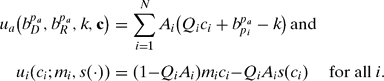
To simplify notation, I henceforth assume without loss of generality that the prosecuting attorney is from party R and label the political benefit from prosecuting a party p official b p.
The subgame perfect Nash equilibria to this game are straightforward, so I defer formal characterization to Lemma 1 in Appendix A. In equilibrium, prosecutors never indict officials against whom no referral is brought. Conditional on observing a referral, the prosecuting attorney will pursue a formal charge against an official if and only the observed level of corruption of an official from party p exceeds a threshold equal to k−b p. Officials fall into one of three relevant categories (a fourth category, described in Lemma 1, is knife's edge): the first consists of those who experience negative marginal utility from corruption (m i < 0) and who therefore do not engage in it (c i* = 0). The second group consists of individuals whose optimal level of corruption given the threat of prosecution falls below the prosecutor's threshold for indictment. These officials will engage in corruption at the threshold level (c i*=k−b p), knowing that even if they are detected, they will not be prosecuted. The remaining officials engage in levels of corruption greater than the prosecutor's threshold; those levels are strictly increasing in the official's type, m i, and decreasing in the probability of referral q.Footnote 14
Empirical Implications and Identification
In this section, I explore the empirical implications of the model, consider potential threats to inferring partisan bias with observational data on corruption prosecutions, and derive a strategy for overcoming these threats. Formal propositions and proofs appear in Appendix A.
The foregoing suggests that a partisan-biased prosecutor will be willing to file weaker cases against political opponents than allies, which will in turn produce lower sentences. Suppose the underlying distribution of official types for party D, g D(⋅), is identical to that of party R, g R(⋅). Partisan bias on the part of a prosecutor from party R should then lead to (1) lower average sentences for defendants from party D than defendants from party R, and (2) a higher proportion of defendants from party D in the set of prosecutions than in the general population.
The assumption that the distribution of benefits to corrupt behavior is the same across the two parties is, of course, unlikely to hold in reality. In the U.S., for example, Democrats tend to be disproportionately concentrated in urban areas, where opportunities for (and rewards to) corruption may be greater. Differences in these distributions threaten to confound efforts to assess bias using cross-sectional data on corruption prosecutions from a given administration.
To make this issue concrete, assume that the party-specific distributions of types are not necessarily equal, but may be ordered by monotone likelihood ratio (MLR) dominance.Footnote 15 Informally, MLR dominance is a common way of characterizing one distribution as “larger” than another; an example would be two normal distributions with the same variance, one of which has a higher mean than the other.Footnote 16 First, suppose g R(⋅) strictly MLR dominates g D(⋅); this would imply officials from party R tend to enjoy higher returns from corruption than officials from party D and will, ceteris paribus, engage in more corrupt activity as a consequence. Given a prosecutor from party R, the expected sentence for officials from party D could be less than the expected sentence for officials from party R in the presence or absence of partisan bias. Figure 2A displays the intuition graphically: the posited difference in distributions will lead to a lower expected level of corruption—and thus lower sentences—from party D than from party R, even when there is no partisan bias on the part of the prosecutor (b D = b R=b). In the presence of partisan bias, it would be impossible to distinguish the effect of the bias from the effect of the difference in the underlying distributions.
Potential Threats to Inferring Bias Stemming from Underlying Interparty Differences in Returns to Corrupt Activity: (A) Confounding Yields Overestimate of Partisan Bias, (B) Confounding Yields Underestimate of Partisan Bias

Next, suppose that g D(⋅) weakly MLR dominates g R(⋅). Given a prosecutor from party R, the expected sentence for officials from party D would be lower than the expected sentence for officials from party R only in the presence of partisan bias. As Figure 2B suggests, dominance of the distribution of party D types pushes the expected sentence for defendants from party D up relative to the expected sentence for defendants from party R. If, in spite of this, we nonetheless observe a significantly lower average sentence for defendants from party D than party R, the source of the difference must be partisan bias.
In terms of estimation, a difference in the underlying party-specific distributions is akin to omitted variables bias (OVB). In the first case, the OVB is away from zero, whereas in the second, the OVB is toward zero. Note that if one is assessing partisan bias of a prosecutor from party D, the potential threats to inference will be reversed: if g R(⋅) dominates g D(⋅), the OVB will be toward zero, whereas if g D(⋅) dominates g R(⋅), the bias will be away from zero.
Rather than assume, implausibly, that the underlying distributions are equal across parties, my identification strategy instead relies on a comparison of corruption case outcomes under both party D and party R prosecutors, under the less stringent assumption that g D(⋅) and g R(⋅) do not change drastically over adjacent administrations.Footnote 17 First, I consider conditions under which one can infer an ordering of the party-specific distributions from the data, which would in turn allow one to sign the OVB. It turns out that patterns in the data would permit this. In particular, if we assume that g D(⋅) and g R(⋅) can be ranked by MLR dominance, then disproportionate targeting of defendants from party D (relative to their proportion in the general population—not the set of referrals) by a prosecutor from party D can occur only if g D(⋅) strictly MLR dominates g R(⋅).
The intuition is simple: the presence of a party D prosecutor will push down the proportion of partisan-affiliated defendants from party D if she is biased, and have no effect on that proportion otherwise. If, in spite of this, we observe that proportion exceed its analog in the general population, then the only possible source of the disproportionality is a discrepancy in the distributions. For similar reasons, disproportionate targeting of officials from party R by prosecutors from party R can occur only if g R(⋅) strictly MLR dominates g D(⋅).Footnote 18 In other words, if we observe disproportionate prosecution of co-partisans by a prosecutor, then differences in observed sentences between the parties under that prosecutor will tend to overstate the extent of that prosecutor's partisan bias (OVB away from zero), whereas differences in observed sentences under a prosecutor from the opposite party will tend to understate the extent of that prosecutor's bias (OVB toward zero).
Second, let E[s|p i, p a] represent the expected sentence of officials from party p i under an administration from party p a. In Appendix A, I demonstrate that the sample analog of the quantity

provides an unconfounded measure of the total extent of partisan bias summed across two adjacent administrations of different parties. Readers may recognize this quantity as a differences-in-differences (DiD). The DiD estimator recovers an unbiased measure of the aggregate effect of partisanship by controlling for (“differencing out”) time-invariant differences between the party-specific type distributions and administration-specific effects (e.g., how much the administration prioritizes public corruption prosecutions generally). Critically, however, the estimator does not permit one to apportion the partisan bias between the two administrations.
Discussion of the Model
Before proceeding to the empirical analysis, I discuss the reasoning behind several important features of the model. First, the model does not distinguish between cases that go to trial and those that result in plea bargains. A simple permutation in which the prosecutor offered the defendant a “take it or leave it” plea bargain to avoid the gamble of a trial and with an exogenously given bargaining breakdown probability would yield results substantively similar to those described previously. Note that in the model, the function s(⋅) represents sentences brought about by plea bargains as well as the expected sentence given the lottery of a full trial; consequently, proper empirical tests for differences in sentencing will include plea bargains, acquittals, dismissals, and guilty verdicts in the calculation of the average observed sentence.
Second, to keep the exposition simple, the model assumes the referral process and the sentence function s(⋅) are not affected by the partisanship of the defendant. With respect to the latter, the fact that federal judges are themselves appointees with political affiliations may call this assumption into question. Later in the article, I discuss my approach for handling this challenge in the empirical analysis. With respect to the former, a plausible case could be made that pressure brought to bear on federal investigators works in the same direction as the partisan bias of the U.S. Attorneys themselves (and, indeed, might be initiated by them). If this is the case, then evidence of partisan bias may be attributed to the Justice Department as a whole, rather than the U.S. Attorneys in isolation.
Third, the model assumes that the referral accurately reflects the level of corruption in which an official engaged. In practice, the referral may contain noise that is (partially or fully) resolved during the discovery period between indictment and a trial. A simple version of the model with uncertainty resolution would have the prosecutor learn the true value of c i conditional on paying the cost k. Such a model would share many features of the model described previously: most important, the prosecutor's strategy would be characterized by a threshold governing whether to indict given the quality of the initial referral, and that threshold would be lower for opponents given partisan bias.
The chief difference between such a model and the one described previously is that these thresholds would incorporate, in addition to any partisan bias, the prosecutor's prior beliefs about a defendant's type. So, for example, suppose the distribution of types from party D dominated the distribution from party R. The prosecutor would respond to this information by lowering the threshold for indictment for party D below that of party R, even in the absence of partisan bias. At the margin—that is, given a referral that makes the prosecutor exactly indifferent between indicting and not indicting—the equilibrium thresholds would exactly offset the difference in the distributions. As an empirical matter, however, we observe the average sentence; uncovering the marginal sentence is considerably more difficult.Footnote 19 To the extent that the model with uncertainty resolution better captures reality, the DiD test for aggregate partisan bias across administrations will be more informative than the tests for determining bias within an administration.
EMPIRICAL RESULTS
Description of Data
To test for systematic partisan bias at the Justice Department, I gathered two samples of state and local corruption prosecutions. The first consists of cases concluded during the Bush administration from 2004 to 2006, during which John Ashcroft and Alberto Gonzales each served as Attorney General. The second consists of cases concluded during the Clinton administration from 1998 to 2000, toward the end of Janet Reno's term as Attorney General. The method employed to compile the data was somewhat involved and is described in detail in Appendix B. These time frames were chosen for two reasons. First, the quality of electronic court records prior to 1998 (particularly in some judicial districts) is dramatically lower than more recent data. Second, using these periods eliminates cases that began under one president and concluded under another. At first glance, such cases may seem particularly attractive, pointing in the direction of a regression discontinuity-type research design. However, my theoretical model offers no coherent predictions for those cases.
For the 2004–2006 sample, I obtained information on the prosecution outcomes of 222 defendants. Before discussing their partisan composition, I note several other interesting features of the data. First, notwithstanding the DOJ's classification of these cases as “official corruption,” 87 of the individuals (39%) are not government officials, but private citizens who may or may not be involved with corrupt officials. These include contractors accused of bribery, party operatives accused of buying votes, and a minister accused of establishing a bogus welfare-to-work program. Second, slightly more than half of the observations (115) are individuals who cannot be readily classified as belonging to one or the other party. In addition to some of the private citizens just mentioned, there are also public officials engaged in routine government operations, such as law enforcement officials (e.g., sheriffs' deputies and probation officers accused of extortion), school superintendents, liquor commission investigators, and water district managers. Officials who can be classified as partisan include mayors and town supervisors, city council members and treasurers, judges, and aides to elected officials. The modal lead charge for defendants is the bribery statute (48 defendants), followed by the Hobbs Act (39), conspiracy to defraud the United States (37), and mail fraud (20). Of the 222 cases, 204 resulted in guilty verdicts: 177 of those from plea bargains and the remainder from jury trials. Approximately two thirds of cases in which the defendant was found guilty (130) resulted in at least some prison time for the defendant. The median length of incarceration given a prison sentence was 21 months. The maximum sentence was 188 months. Of the remaining 18 cases, six were dismissed and 12 concluded with the defendant's acquittal at trial.
There are 223 cases in the 1998–2000 sample. Sixty-six of these were private citizens, and 77 could be readily classified as having a partisan affiliation. Violations of the Hobbs Act constituted the modal lead charge (72 defendants), followed by violations of the bribery statute (56). Of the 210 cases resulting in guilty verdicts, 175 emerged from plea bargains. Seven cases ended with not guilty verdicts, and six with dismissals. Interestingly, a slightly larger proportion of guilty verdicts in the Clinton sample ended in incarceration: 157, or 75%. Of those cases, the median sentence was 24 months, and the maximum 488 months.Footnote 20
Partisan Composition of Defendants
Table 1 displays information on the partisan breakdown of defendants in the two sampling periods. Of the 222 cases for which I have collected data in the 2004–2006 (Bush administration) period, 84 of these individuals could be identified either as Democrats or as affiliated with a Democratic politician (e.g., in a fraudulent transaction). In contrast, only 23 defendants could be classified as either Republican or Republican affiliated. The ratio of 3.65 Democrats to 1 Republican prosecuted echoes the discrepancy observed in the Shields/Cragan study cited previously. The discrepancy becomes even more pronounced if one restricts attention to public officials: over six times as many Democratic public officials are observed in the data as Republican.
Partisan Affiliation of Public Corruption Prosecution Defendants, Bush and Clinton Samples

How do these figures differ from the partisan breakdown of defendants prosecuted under Clinton? Of the 223 cases coded, 77 could be identified with one of the two major parties: 49 Democrats and 28 Republicans. The data indicate that Democrats were disproportionately represented in the sample of defendants relative to Republicans in a Democratic administration. Among all defendants, there were 1.75 times as many Democratic-affiliated defendants as Republican-affiliated ones. Restricting attention to public officials, this ratio climbs to 2.6 to 1.
While I lack precise data on the ratio of Democrats to Republicans in the general population, it is not controversial to assume, based on extant surveys during the period, that the ratio was less than 1.8:1.Footnote 21 The overrepresentation of Democrats in the set of prosecutions under Clinton, although less pronounced than under Bush, suggests that disproportionality cannot by itself be taken to indicate anti-Democratic bias or “profiling” by the Bush administration in corruption prosecutions.
More important for current purposes, the fact that Democrats appear to be disproportionately prosecuted by the Clinton administration, provides evidence that the benefit to engaging in corruption typically tends to be larger at the state and local levels for Democrats than for Republicans. Employing the criteria discussed previously, this pattern in the data allows me to assess the direction in which the following results might be confounded: in particular, estimates of sentencing disparities are likely to overstate the true extent of partisan bias in the Clinton Justice Department, whereas those estimates are likely to understate the true extent of partisan bias in the Bush Justice Department.
Descriptive Results
Having assessed an important issue of potential confounding, I next turn to the specific prediction that in the presence of prosecutorial partisan bias, the average sentence of prosecuted partisan opponents will tend to be lower than that of prosecuted allies. Results appear in Table 2. Because sentences involving probation are not scalable on the same metric as those involving incarceration, I employ two different measures of total punishment. Columns (1) through (3) consider prison sentences in months, treating defendants who received probationary sentences as equivalent to those who were acquitted. In contrast, columns (4) through (6) incorporate information on the length of probationary sentences, under the uncontroversial assumption that the most severe probationary sentence (60 months) is more lenient than the least severe incarcerative sentence (one month). How the “pain” associated with an extra month of probation compares with that of an extra month of prison is unknown, so I present an intermediate case in which an extra month of prison is assumed to be five times as painful. So, for example, five years (60 months) probation would be coded as 12 units of punishment, and one month of incarceration as 13. Results employing different “exchange rates” between prison and probation are qualitatively similar to those reported here. Columns (1) and (4) in Table 2 display average sentences for different categories of defendants with identifiable partisan affiliations prosecuted under the two administrations, using the two measures of punishment. Interestingly, the data suggest that the average prison sentence for partisan-affiliated public corruption defendants under the Bush DOJ (22 months) was slightly longer than under Clinton (16 months), although this difference is not statistically significant.
Descriptive Indicators of Partisan Bias in Sentencing: Administration-specific Differences Between Republican and Democratic Defendants and Differences-in-Differences

Notes: Sentences and differences in columns (1) through (3) denote months of incarceration placing zero value on probation; sentences in columns (4) through (6) are calculated as 0.2 times the number of months of probation in the sentence if the sentence is solely probationary, and 12 plus the number of months of incarceration plus 0.2 times the number of months of probation if the sentence includes imprisonment (see text for additional explanation). One-tailed p values in parentheses.
Next, I turn to tests of administration-specific sentencing differences, reported in columns (2) and (5) of Table 2. The numbers in parentheses are one-tailed p values for corresponding t tests assuming unequal variances. (One-tailed tests are appropriate given the directional nature of the hypotheses tested.) For differences between Republican and Democratic average sentences during the Bush administration, a positive difference is evidence of partisan (pro-Republican) bias, as it is consistent with prosecution of weaker cases against Democrats. Turning to the results for the Bush administration, we find a positive difference pooling across all defendants, consistent with anti-Democratic or pro-Republican bias. However, the pooled results miss statistical significance at conventional levels. Confining attention to the sentences of public employees, however, the difference in means is statistically significant. This difference is substantively large as well: for example, the average imprisonment under Bush for Republican public employees is nearly twice that of the Democratic average.Footnote 22 Confining attention to private citizens with partisan affiliations, differences are quite small and nowhere close to significant. Results employing the alternative punishment measure incorporating probation are broadly similar to those using the imprisonment measure.
For differences between Republican and Democratic average sentences during the Clinton administration, a negative difference is evidence of partisan (pro-Democratic) bias. Pooling over all defendants with identifiable partisan leanings, the data indicate that Democrats received prison sentences approximately six months more severe than Republicans. This difference is statistically significant for both punishment measures reported in Table 2. Confining attention to public employees only, differences are highly significant and of the anticipated sign. Under Clinton, Democratic officials received sentences 10 to 11 months more severe than Republican officials on average.
The data are thus consistent with partisan bias in the prosecution of public officials in both the Clinton and Bush administrations; however, they do not indicate partisan bias in the prosecution of private citizens. Taken together with the results in the previous section concerning confounding, the evidence suggests that observed differences under Bush are attributable to partisan bias and not to underlying differences between defendants from the two parties. The observed differences under Clinton may, however, be wholly or party attributable to such differences.
I report DiD estimates in columns (3) and (6). A positive, significant DiD reflects high total partisan bias summed across the Clinton and Bush administrations. Pooling across all defendants with identifiable partisan affiliations, I detect large, positive effects with both measures of punishment. Confining attention exclusively to public officials prosecuted under public corruption statutes, one observes effects even more pronounced, both in their magnitude and their statistical significance. Across the two administrations, the DiD estimates imply between 30- and 40-month aggregate differences in sentences attributable to partisan bias. As the p values in Table 2 indicate, these effects are very precisely estimated. Last, I detect no significant aggregate partisan effects when confining attention to private citizens.
Conditioning on Covariates
The foregoing analysis assumes that conditional on the partisan affiliation of the defendant, individual cases are exchangeable. In fact, there may be other features of the legal and political environment that affect sentencing. For example, prosecutors may get greater recognition from prosecuting elected officials than private citizens or administrative functionaries. Likewise, prosecutors may obtain scale economies from going forward with cases involving multiple defendants. Finally, judges, who must approve all sentences whether they follow plea bargains or guilty verdicts at trial, are themselves political appointees and may differ in their attitudes toward sentencing.
To account for this potential heterogeneity in cases, I assess the robustness of the descriptive results via three different statistical approaches: least squares regression, exact matching, and genetic matching.Footnote 23 These approaches permit me to estimate the average treatment effect of being a Republican defendant as compared to a Democratic defendant conditional on the previously mentioned features of the environment. The included covariates are whether the defendant was a private citizen, whether he or she was an elected official, whether the sentence was approved by a judge appointed by a Democratic president, and whether the sentence was part of a case with multiple defendants. Because case priorities may vary by the region of the U.S. Attorney's Office (Eistenstein 1978), I also match on regional indicators: Midwest, Northeast, and South (the excluded category is the West). Heteroscedasticity-consistent standard errors are reported for the regression estimates, and bias-corrected standard errors (Abadie and Imbens 2006) for the matching estimates.
In the first four columns of Table C.1 in Appendix C, I report pre- and postmatching balance statistics as a means of diagnosing the success of the genetic matching procedure. (By definition, exact matching entails perfect balance.) Specifically, I employ standardized mean differences and p values for a t test that the covariate means are equal across defendant partisan affiliation (Imai, King, and Stuart Reference Imai, King and Stuart2008; Sekhon n.d.). Balance is indicated by smaller mean differences and larger p values. The diagnostics suggest that excellent balance is obtained on these covariates in both the Bush and Clinton samples. For example, the lowest p value after matching is .7 in the Bush sample and .37 in the Clinton sample.
Table 3 displays estimates for the average effect of being a Republican defendant compared to a Democrat using regression and matching approaches.Footnote 24 Estimates from all three approaches confirm the descriptive results described previously. Pooling over public officials and private citizens, we continue to observe higher sentences for Republicans than Democrats under Bush and lower sentences for Republicans under Clinton, as well as large and highly significant DiD estimates. The most substantial departures from the descriptive results occur in the exact matching estimates, which boost the estimated treatment effect of being a Republican under Bush to more than 27 months. One is hesitant to make too much of this difference, however, because obtaining exact matches requires discarding more than 40% of the cases in the sample.
Regression and Matching Estimates of Administration-specific Differences in Sentences Between Republican and Democratic Defendants and Differences-in-Differences, Excluding Crime-level Covariates

Notes: See notes in Table 2 and text for description of measure incorporating probation. Heteroscedasticity-consistent standard errors reported for regression estimates; Abadie and Imbens (Reference Abadie and Imbens2006) standard errors employed for matching estimates, with standard errors for differences-in-differences matching estimates calculated assuming independence of Bush and Clinton samples.
Note that I do not include controls for observable features of the underlying crime in the list of covariates. This omission is made to avoid posttreatment bias, which can emerge if the analyst controls for variables that are causally dependent on the treatment variable of interest (in this case, the partisanship of the defendant). The theoretical model implies that the distribution of criminal activity itself is, in the presence of bias, affected in equilibrium by the partisanship of the defendant. The sentence is simply a noisy measure of that criminal activity. Other features of crimes aside from the sentence are also dependent on the defendant's partisanship; thus, controlling for them may bias the estimated effect of partisanship.
Nonetheless, it is still useful to see whether matching on these features of the cases changes anything. I therefore reran the analysis from Table 3, including three indicator variables for whether the top charge in the indictment was Racketeering, Fraud, or Bribery (the excluded category is Obstruction of Justice). Balance statistics for the genetic matching appear in the fifth through eighth columns of Table C.1 in Appendix C. Results for regression and matching analysis incorporating crime-level covariates are displayed in Table C.2 in Appendix C, and are quite similar to the estimates that do not include them in the list of covariates. Note that exactly matching on the type of crime drastically reduces the sample size by more than 75%; in fact, in the analysis of sentences of private citizen defendants under Clinton, only four exact matches could be found.
Heterogeneity Across U.S. Attorneys' Offices
The foregoing analysis is premised on the assumption that it is possible to assess the extent of partisan bias in the Justice Department taken in toto. The decision to prosecute a public corruption cases, however, lies largely with the individual U.S. Attorneys and their assistants, who may exercise autonomy in setting office priorities. Accordingly, any heterogeneity in the extent of partisan bias among different U.S. Attorneys may manifest itself in variation across districts in differences in the observed sentences of Republican and Democratic public corruption defendants.
Ideally, one would estimate sentencing differences (and DiDs) for every U.S. Attorney's Office. However, many of the districts have only one or a handful of cases associated with them. An alternative approach is to model heterogeneity in the effects of partisan bias parametrically, in the context of a random coefficient model (see, e.g., Gelman and Hill Reference Gelman and Hill2007, ch. 11), in which district-level differences in Republican and Democratic corruption sentences are assumed to be draws from a normal distribution whose estimated mean and standard deviation reflect, respectively, the typical effect and the extent of heterogeneity.
Table 4 displays estimates from a series of such models. In addition to the estimate of the mean partisan effect, its standard error, and the one-tailed p value, I also report, in columns (4) and (8) the estimated standard deviation of the distribution of partisan differences. Estimates of the mean effect of defendant party and the uncertainty surrounding them are quite similar to the models estimated assuming homogeneous effects across districts. Two features of these estimates are particularly noteworthy, however. First, the magnitude of estimated standard deviation of the effects across districts in the pooled (public and private) sample suggests considerable variation in the differences in sentences for Republican and Democratic defendants. To see which districts departed most significantly from the mean effect, I calculated best linear unbiased predictors for district-level party effects. In the Bush data, the districts of Connecticut, Western North Carolina, and Western Tennessee showed unusually small (but still positive) differences between Republican and Democratic defendants, whereas Eastern California and Northern Illinois featured the largest differences. Interestingly, none of the dismissed U.S. Attorneys served in those districts. In the Clinton data, Southern Florida and Eastern New York displayed unusually small (but still negative) differences, and the difference for Western Oklahoma was the wrong (i.e., positive) sign. Differences for Northern Alabama, Northern Illinois, and Southern Ohio were atypically large in magnitude.
Accounting for Interdistrict Heterogeneity: Random Coefficient Model Estimates of Administration-specific Differences in Sentences Between Republican and Democratic Defendants and Differences-in-Differences, Excluding Crime-level Covariates

Notes: See notes in Table 2 and text for description of measure incorporating probation. Standard errors for differences-in-differences estimates calculated assuming independence of Bush and Clinton samples.
Second, restricting attention to public employee defendants only, the variance of effects across districts remains large for the Bush administration, but is quite small for the Clinton administration. In fact, a likelihood ratio test comparing the random coefficient model to simple linear regression for the Clinton/public employee sample is right at the threshold of rejecting the latter (χ2 = 4.48, p = .11). The apparently greater homogeneity in effects across districts under Clinton relative to Bush is intriguing, and suggests an avenue for future research on the extent of administrative centralization under each.
Although limitations in the data preclude estimating separate sentencing differences for most districts, an important exception to this rule is the Northern District of Illinois, which handles corruption cases from Chicago and its surrounding suburbs. I have data from this district on Democratic and Republican defendants under both the Bush and Clinton administrations. Northern Illinois is also a “hard case” for demonstrating partisan bias because of the reputation of Bush-appointed U.S. Attorney Patrick Fitzgerald for nonpartisanship. The U.S. Attorney for Northern Illinois from 1998 to 2000 was Clinton appointee Scott Lassar.
Table 5 displays the results of regression and matching analyses employing cases only from the Northern District of Illinois. Because of the small sample size, I report only results pooling across both public and private defendants. (Balance statistics for the genetic matching appear in Table C.1 in Appendix C. The procedure failed to produce good balance on the party of the president who appointed the presiding judge in a case.) The results for the single district mirror those for the national sample. We observe Republican defendants receiving substantially and statistically significantly higher sentences under Fitzgerald, and Democrats receiving higher sentences under Lassar. One challenge associated with focusing attention on this particular district is the fact that Democratic-affiliated defendants tend to work in Chicago government, whereas Republican-affiliated defendants tend to work for the state or come from smaller towns such as Cicero. Of course, these differences tend to persist across administrations, affording validity to the DiD estimates as evidence of partisan bias aggregated across the two administrations.
Regression and Matching Estimates of Administration-specific Differences in Sentences Between Republican and Democratic Defendants and Differences-in-Differences, Northern District of Illinois Only

Notes: See notes in Table 2 and text for description of measure incorporating probation. Heteroscedasticity-consistent standard errors reported for regression estimates; Abadie and Imbens (Reference Abadie and Imbens2006) standard errors employed for matching estimates, with standard errors for differences-in-differences matching estimates calculated assuming independence of Bush and Clinton samples.
DISCUSSION
Some Remaining Issues Addressed
Here, I address some remaining challenges to the validity of the model and empirical findings. First, although the model allows for prosecutorial discretion in case selection, it does not consider discretion over what sentence to push or bargain for—presumably, a biased prosecutor would push for more severe sentences against opponents than allies. It is immediate that this behavior would work against my empirical strategy for detecting partisan bias. For example, the model anticipates that under a biased Republican prosecutor, the typical sentence should be lower for Democrats than Republicans, ceteris paribus. Discretion of the sort considered by this objection would push the average sentence for Democrats up and the average sentence for Republicans down. If, in spite of this, we still observe Democrats receiving lower sentences under a Republican prosecutor, the source of this difference is likely to be the bias in case selection considered explicitly in the model (accounting for the possibility of confounding effects discussed previously).
The second issue concerns professional norms of neutrality in their application of the law. Suppose U.S. Attorneys, in an effort to appear politically neutral, devote their limited time toward building a few strong, high-profile cases against officials from their own party. The empirical implications would be similar to those anticipated by my model in the presence of partisan bias. There are two responses to this concern. To begin, it is not clear whether a prosecutor trying to appear neutral would actually benefit from adopting this strategy rather than prosecuting many smaller cases against co-partisans. The posited strategy would open the prosecutor to the very charge of bias (supported by evidence of disproportionality, which is easier to observe than the prosecutor's allocation of costly effort) that she had sought to avoid. Moreover, although prosecutors may be sensitive to professional norms of neutrality, it is unlikely that their political superiors are. Consequently, if prosecutors truly behaved in the posited way, we would expect to see Republican administrations exhibiting a systematic preference for appointing Democratic U.S. Attorneys, and vice versa. The fact that we do not observe this further mitigates against this alternative account.
Third, my analysis examines cases concluded relatively late in the Clinton and Bush administrations. Suppose that U.S. Attorneys tend to prioritize cases against partisan opponents early in their administrations. It could then be that the differences I observe are simply a consequence of the Justice Department having already completed the strongest cases against its opponents. In fact, this is unlikely to be the case. To begin with, it is not the case that each administration starts with a finite supply of corruption cases that it depletes over time; the set of matters under consideration by U.S. Attorneys is constantly replenished by a steady stream of new referrals from investigative agencies. Moreover, the most high-profile cases tend to be those that stretch out over years; thus, for example, some convictions or plea agreements reached in 2006 were initially filed in 2001. Nonetheless, to make sure that these dynamic effects do not drive my results, I divided the data into “early” (1994–1996 and 2001–2003) and “late” (1998–2000 and 2004–2006) strata and reran my analysis for each. If the objection is correct, we would expect to see the partisan differences anticipated by the theory muted for the early strata relative to the late ones. In fact, we observe precisely the opposite.
Implications for the Study of Politicization and Autonomy
Contemporary theories of bureaucratic politics emphasize the tension between the partisan loyalties and expertise of officials. Lewis (Reference Lewis2008), for example, argues that a president will be more apt to politicize agencies (foregoing the opportunity to capitalize on careerist expertise) when careerists do not share his or her underlying policy preferences. Consequently, whether an administration will politicize an agency may depend as much on which administration as on which agency. To the extent that an agency fosters professional norms devoted to the neutral application of the law (e.g., Huber Reference Huber2007), however, presidents from both parties may benefit from seeking to politicize. The evidence presented in this article is consistent with politicization attempts by both Bush and Clinton, although it is not possible to definitively assess relative politicization between the two administrations.
At the same time, accounts of policy making at both the Justice Department (Seymour Reference Seymour1975) and elsewhere (Carpenter Reference Carpenter2001) point to agency culture when accounting for the success of some agencies in some periods at resisting efforts at politicization. To be sure, a strong culture is not an insurmountable obstacle: several U.S. Attorneys have cited their defense of department culture as an immediate cause of their dismissals. More generally, the causal antecedents of strong bureaucratic culture are complex. Carol Lam, one of the fired U.S. Attorneys, suggested that the terminations “so transgressed the unwritten understanding and traditions of the department that, ironically, I think it has now reinforced them” (Fisher Reference Fisher2007). Another fired attorney, David Iglesias, was less sanguine about the department's resilience, writing that “it will take time for the damage done to the Justice Department to be completely remedied” (Iglesias Reference Iglesias and Seay2008, 232).
Finally, to the extent that politicization efforts, once uncovered, can damage an administration politically, it is worth considering the potential role of oversight by either Congress or the media. The U.S. Attorney firing scandal would likely not have received as much attention if the majority control of Congress had not changed in 2006. In this vein, it is worth noting that the sample of corruption prosecutions from the Clinton administration employed in this article was drawn from a period of divided government and intense congressional scrutiny of the Reno Justice Department. It is possible that the mere potential for such scrutiny mutes the incentive to politicize the administration of justice for partisan ends. Likewise, the Bush sample was drawn from a period of unified government. A valuable extension, albeit one beyond the scope of the current article, would be to examine Clinton administration corruption prosecutions during unified Democratic control of government and Bush administration prosecutions during divided government, to better understand this effect.
Conclusion
The 2007 U.S. Attorney firing scandal raised the possibility that federal corruption laws could be deployed for partisan ends. In this article, I have sought to move beyond anecdotes to construct a systematic test of partisan bias in corruption prosecutions. My simple theoretical model anticipates differences in the distribution of observed sentences between defendants from the two major parties in the presence of partisan bias. Based on estimates of those differences, I find strong evidence of aggregate partisan bias across the Justice Departments of Bill Clinton and George W. Bush. Apportioning the bias between the administrations is slightly more challenging. Although evidence of bias is detected under both administrations, these estimates are susceptible to confounding because we cannot directly observe the actual magnitude of the benefit to an individual of engaging in corruption apart from the (potentially incomplete) evidence on which the prosecutor relies. However, under a plausible set of assumptions, evidence pointing to the disproportionate prosecution of Democrats under both Bush and Clinton speaks to the direction of this confounding effect, implying that the effect of partisanship is most likely stronger than implied by my analysis of Bush-era prosecutions, and weaker than implied by my analysis of Clinton-era prosecutions.
I conclude by noting that these results may be interpreted as both good news and bad news for Democrats and Republicans alike. For Democrats, the evidence suggests that the Bush Department of Justice may indeed have discriminated against them. For Republicans, the fact that Democrats were disproportionately targeted under both Clinton and Bush is evidence that Democrats at the state and local level may have access to more substantial opportunities for corruption than Republicans. This is perhaps not surprising given the concentration of Democratic public officials in urban areas. It is important to keep in mind, however, that the presence of opportunities for corruption for some members of a party is not synonymous with a tendency of the typical official from that party to violate the law. Indeed, both the model and data are fully consistent with compliance by the vast majority of officials and private citizens from both parties.
APPENDIX A: FORMAL RESULTS
I begin with a formal characterization of equilibrium to the game described in the text:
lemma 1 (Equilibrium Characterization). In any subgame perfect Nash equilibrium to the game:
(a) The prosecutor prosecutes official i if and only if i is referred and c i > k − b p; and
(b) For any official i ∈ 1, . . ., N:
![\begin{enumerate}
\item[(i)] $c_i=0$ if $m_i<0$,
\item[(ii)] $c_i\in [0,k-b_p]$ if $m_i=0$,
\item[(iii)] $c_i=k-b_p$ if $m_i\in(0,\frac{q}{1-q}s'(k-b_p)]$, and
\item[(iv)] $c_i = s'(\frac{(1-q)}{q}m_i)^{-1}$ if $m_i\in(\frac{q}{1-q}s'(k-b_p),\infty)$.\end{enumerate}](data:image/gif;base64,R0lGODlhAQABAIAAAMLCwgAAACH5BAAAAAAALAAAAAABAAEAAAICRAEAOw==)
![\begin{enumerate}
\item[(i)] $c_i=0$ if $m_i<0$,
\item[(ii)] $c_i\in [0,k-b_p]$ if $m_i=0$,
\item[(iii)] $c_i=k-b_p$ if $m_i\in(0,\frac{q}{1-q}s'(k-b_p)]$, and
\item[(iv)] $c_i = s'(\frac{(1-q)}{q}m_i)^{-1}$ if $m_i\in(\frac{q}{1-q}s'(k-b_p),\infty)$.\end{enumerate}](https://static.cambridge.org/binary/version/id/urn:cambridge.org:id:binary:20151024011237888-0055:S0003055409990207_eqnU3.gif?pub-status=live)
proof. The game is solved via backward induction. To establish (a), note that if i is not referred, under the assumption that k > b p, the marginal utility to the prosecutor associated with bringing a case against i is b p − k < 0, so not prosecuting strictly dominates prosecuting. From the prosecutor's best response correspondence, if i is referred, the prosecutor strictly prefers prosecuting if c i > k − b p, strictly prefers not prosecuting if c i < k − b p, and is indifferent if c i = k−b p.
To establish part (b)(i), note that if m i < 0, official i's expected utility is strictly decreasing in c i, making c i = 0 a dominant strategy. Next, consider officials for whom m i ≥ 0. Let π(c i) be the probability the prosecutor prosecutes an official engaged in corruption c i given a referral, and suppose the prosecutor does not prosecute if c i = k−b p (i.e., π(k−b p) = 0). The expected utility to official i of engaging in corruption c i is

The official's first-order condition is given by

Suppose a candidate solution to Equation (A.1),  , exceeds k−b p, so, via part (a),
 = 1 and
 = 0. Substituting into Equation (A.1) and solving for ĉ i(⋅) yields the optimal value of c i given in part (b)(iv). (Second-order conditions guarantee a unique maximum.) By assumption, s′(c i)>0, s″(c i)>0, and s′(0) = 0, so s′(⋅)−1 exists and is strictly increasing, with s′(0)−1 = 0. This implies ĉ i(m i;q, s(⋅)) is increasing in m i, with ĉ i(0;q, s(⋅)) = 0. Consequently, there exists an m i′ such that for all m i>m i′, ĉ i(m i;q, s(⋅))>k−b p. Substituting the value obtained for ĉ i(m i;q, s(⋅)) into this inequality and solving yields the condition in part (b)(iv).
For values of m i ∈![$(0,\frac{q}{1-q}s'(k-b_p)]$](https://static.cambridge.org/binary/version/id/urn:cambridge.org:id:binary:20151024011237888-0055:S0003055409990207_inline7.gif?pub-status=live) , ĉ i(m i;q, s(⋅))<k−b p, in which case π(ĉ i(⋅)) = 0. In such cases, the official can always benefit from increasing his level of corruption up to c i = k−b p given π(k−b p)=0, establishing part (b)(iii). Officials for whom m i=0 are indifferent between not engaging in corruption and engaging in any level of corruption up to k−b p given π(c i)=0 for any c i≤ k−b p, establishing part (b)(ii).
To see why any strategy profile that includes π(k−b p)≠0 cannot be an equilibrium, suppose otherwise. Then, for any official with type m i ∈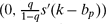 playing strategy c i′<k−b p, there exists an ϵ > 0 such that such an official would benefit from playing c i′ + ϵ.
Let N p be the total number of party p officials in the population, and  the number of officials from party p i prosecuted by a prosecutor from party p a. Let h D(c) be the density of prosecuted corruption levels for party D, and h R(c) the density for party R. The next result summarizes empirical implications of the model under the assumption that party D and party R types are drawn from the same distribution:
Proposition 1 (Empirical Implications Given Equal Type Distributions). Suppose g D(m)=g R(m) for all m. In the presence of a biased prosecutor from party R, (a) the expected sentence for a defendant from party D will be less than the expected sentence for a defendant from party R; and (b) in expectation, the proportion of prosecuted officials from party D will exceed its analog in the population.
proof. (a) From part (a) of Lemma 1, the distribution of prosecuted corruption levels will be left truncated at k−b p for officials from party p. From part (b)(iv), corruption levels prosecuted with positive probability are a strictly increasing function of an official's type m i and are independent of b p. Consequently, if g D(⋅)=g R(⋅), h D(c) and h R(c) will both be left-truncated manifestations of the same underlying density, and the expected level of corruption will be lowest for the party with the lower truncation point—party D in the presence of partisan bias (b D > b R). Because s(⋅) is a strictly increasing function of c, this in turn implies that the expected sentence for prosecuted officials from party D will be less than the expected sentence from party R.
(b) From Lemma 1, the probability an official from party p engages in a prosecutable level of corruption given a prosecutor from party R is given by
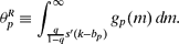
If g D(⋅) = g R(⋅), then  if and only if the prosecutor is biased (b D > b R), in which case

where  is the observed number of prosecuted officials from parties D and R.
Let  and
 denote, respectively, weak and strict monotone likelihood ratio orderings. The next result characterizes threats to inference stemming from differences in g D(⋅) and g R(⋅):
Proposition 2 (Potential Threats to Inference). Given a prosecutor from party R:
(a) If g D(⋅)
g R(⋅), then the expected observed sentence for officials from party D will be smaller than the expected observed sentence for officials from party R only in the presence of partisan bias (b D > b R); and(b) If g R(⋅)
g D(⋅), then the expected observed sentence for officials from party D could be smaller than the expected observed sentence for officials from party R in the presence or absence of partisan bias (b D ≥ b R).
proof. Note two useful properties of the monotone likelihood ratio order: (1), it is preserved under truncation; and (2), if the density of a random variable X MLR dominates that of random variable Y, then the density of ψ(X) MLR dominates that of ψ(Y) for any increasing function ψ(⋅) (see Theorems 1.C.6 and 1.C.8 of Shaked and Shanthikumar Reference Shaked and Shanthikumar2007).
The conjunction of these two properties and part (a) of Lemma 1 imply that in the absence of partisan bias (b D = b R), if g D(⋅) g R(⋅), then the distribution of party D sentences will weakly MLR dominate the distribution of party R sentences. But then the expected observed sentence for party D will be weakly larger than that of party R. The only means for this inequality to be reversed is for the lower bound of the support of prosecuted corruption levels (and thus sentences) to be lower for party D than party R, which can only occur given partisan bias (b D > b R). In contrast, if g R(⋅) g D(⋅), then in the absence of partisan bias the expected observed sentence for party R will exceed that of party D, and the presence of partisan bias will reenforce this difference.
The following result gives conditions under which an ordering of g D(⋅) and g R(⋅) may be inferred from disproportionatility in the data:
Proposition 3 (Sufficient Conditions for Ordering Type Distributions). Suppose g D(⋅) and g R(⋅) can be ordered by monotone likelihood ratio dominance. Then disproportionate targeting of party R by prosecutors from party R will occur in expectation only if g R(⋅) g D(⋅). Likewise, disproportionate targeting of party D by prosecutors from party D will occur in expectation only if g D(⋅)g R(⋅).
proof. Assume a prosecutor from party R. There are two cases to consider: first, suppose the prosecutor is unbiased (b D=b R). If g D(⋅) g R(⋅), then via Equation (A.2), party D officials will be prosecuted with weakly higher probability than party R officials. If g R(⋅) g D(⋅), party R officials will be prosecuted with strictly higher probability than party D officials. Second, suppose the prosecutor is biased (b D > b R). Then the lower threshold for officials from party D (see Lemma 1 and Proposition 1) will entail an increase in the probability party D officials are prosecuted relative to the probability party R officials are prosecuted. g D(⋅) g R(⋅) will further increase the probability for party D officials relative to party R officials. In contrast, if g R(⋅) g D(⋅), the effect of the ordering of the densities will be to to increase the probability party R officials are prosecuted relative to party D officials. The conjunction of these effects could lead to disproportionate prosecution of party R, party D, or neither. Consequently, disproportionate prosecution of party D officials is consistent with any ordering of g D(⋅) and g R(⋅), whereas disproportionate targeting of party R officials is consistent only with g R(⋅) g D(⋅). An analogous proof establishes the proposition for a party D prosecutor.
The final result motivates the DiD estimator described in the text:
Proposition 4 (Aggregate Effect of Partisan Bias). Suppose the party-specific distributions of official types, g D(⋅) and g R(⋅), remain stable across two adjacent administrations of different parties. Then, partisan bias exists within at least one of those administrations if and only if
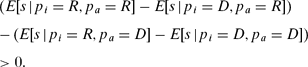
proof. Consider the following model of the conditional expected sentence for defendant i:

where I(⋅) is an indicator function, γp i captures the effect on the expected sentence of the underlying distribution of official types in party p i, αp a captures the effect of prosecutorial priorities under a prosecutor from party p a, βDR is the diminution of sentences attributable to partisan bias by a prosecutor from party R against officials from party D, and βRD is the diminution attributable to bias by a party D prosecutor against party R defendants. Then, E[s|p i = R, p a = R] = γR + αR, E[s|p i = D, p a = R] = γD + αR −βDR, E[s|p i = R, p a = D] = γR + αD − βRD, and E[s|p i = D, p a = D = γD + αD. Substituting into inequality Equation (A.3) and simplifying yields βDR + βRD, which is the sum of the effects of partisan bias across the party D and party R administrations.
APPENDIX B: DATA COLLECTION
The Executive Office of U.S. Attorneys (EOUSA) releases data on prosecutions to two forums: TRAC, cited previously, and the Federal Justice Statistics Resource Center, a subdivision of the Bureau of Justice Statistics (BJS), co-sponsored by the Urban Institute. Although each database contains information on the same universe of cases, each has advantages. For example, TRAC contains DOJ program categories, whereas BJS data contain readily accessible information on case priority: District (D), National (N), or Both National and District (B). I restrict attention to categories N and B (priority D cases are typically clerical workers). Neither data source has the defendant's name. The data universe for this article consists of the intersection of BJS records of the relevant priority levels and TRAC records with DOJ categorized as state and local corruption for the years under consideration.
To locate defendant names, I relied on the federal district courts' Case Management/Electronic Case Files (CM/ECF) system and, when necessary, Nexis. This process was fairly involved. The first step was to enter the filing date from the EOUSA data into a district's CM/ECF system. This typically yielded a list of cases. The second step was to restrict attention to cases in which the United States was a plaintiff and in which the CM/ECF closing date approximated the TRAC closing date. The third was to examine the electronic docket to find the case whose details matched those summarized in TRAC. From there, I obtained the defendant name(s). If this approach did not work, I searched Nexis for articles in state news sources that included the judge's name around the time of sentencing, then searched for the name of the defendant listed in the news story in CM/ECF.
Finally, using the defendant's name and common variants thereof, I obtained information on his or her position and party using Nexis, searching U.S. Attorney press releases, election returns, telephone calls to local city halls, or the Internet more broadly. (A list of sources is available on request.) This approach identified approximately 83% of the defendants.
APPENDIX C: ADDITIONAL TABLES
Balance Tests for Covariates Used in Genetic Matching Analyses on Pooled Samples of Public and Private Defendants

Regression and Matching Estimates of Administration-specific Differences in Sentences Between Republican and Democratic Defendants and Differences-in-Differences, Including Crime-Level Covariates

Notes: See notes in Table 2 and text for description of measure incorporating probation. Heteroscedasticity-consistent standard errors reported for regression estimates; Abadie and Imbens (Reference Abadie and Imbens2006) standard errors employed for matching estimates, with standard errors for differences-in-differences matching estimates calculated assuming independence of Bush and Clinton samples.
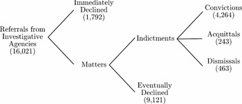
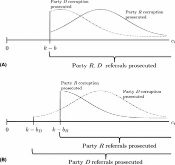
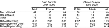
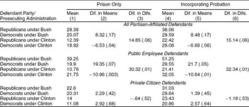
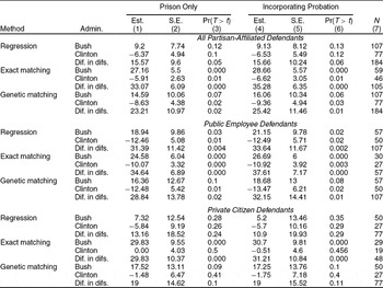
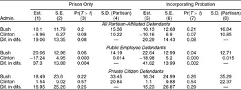
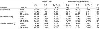
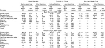
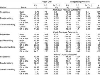



Comments
No Comments have been published for this article.