Resolvent-based study of compressibility effects on supersonic turbulent boundary layers

H. Jane Bae; Scott T. M. Dawson; Beverley J. McKeon

doi:10.1017/jfm.2019.881

Resolvent-based study of compressibility effects on supersonic turbulent boundary layers

Published online by Cambridge University Press: 26 November 2019

and

H. Jane Bae*: Affiliation:
Graduate Aerospace Laboratories, California Institute of Technology, Pasadena, CA91125, USA
Scott T. M. Dawson: Affiliation:
Graduate Aerospace Laboratories, California Institute of Technology, Pasadena, CA91125, USAMechanical, Materials and Aerospace Engineering Department, Illinois Institute of Technology, Chicago, IL60616, USA
Beverley J. McKeon: Affiliation:
Graduate Aerospace Laboratories, California Institute of Technology, Pasadena, CA91125, USA
*: †Email address for correspondence: hjbae@caltech.edu

Article contents

Abstract
Introduction
Resolvent formulation of compressible zero-pressure-gradient turbulent boundary layer
Characteristics of resolvent modes for compressible turbulent boundary layer
Scaling of the principal singular value and resolvent modes
Conclusions
References

Rights & Permissions

Abstract

The resolvent formulation of McKeon & Sharma (J. Fluid Mech., vol. 658, 2010, pp. 336–382) is applied to supersonic turbulent boundary layers to study the validity of Morkovin’s hypothesis, which postulates that high-speed turbulence structures in zero-pressure-gradient turbulent boundary layers remain largely the same as their incompressible counterparts. Supersonic zero-pressure-gradient turbulent boundary layers with adiabatic wall boundary conditions at Mach numbers ranging from 2 to 4 are considered. Resolvent analysis highlights two distinct regions of the supersonic turbulent boundary layer in the wave parameter space: the relatively supersonic region and the relatively subsonic region. In the relatively supersonic region, where the flow is supersonic relative to the free-stream, resolvent modes display structures consistent with Mach wave radiation that are absent in the incompressible regime. In the relatively subsonic region, we show that the low-rank approximation of the resolvent operator is an effective approximation of the full system and that the response modes predicted by the model exhibit universal and geometrically self-similar behaviour via a transformation given by the semi-local scaling. Moreover, with the semi-local scaling, we show that the resolvent modes follow the same scaling law as their incompressible counterparts in this region, which has implications for modelling and the prediction of turbulent high-speed wall-bounded flows. We also show that the thermodynamic variables exhibit similar mode shapes to the streamwise velocity modes, supporting the strong Reynolds analogy. Finally, we demonstrate that the principal resolvent modes can be used to capture the energy distribution between momentum and thermodynamic fluctuations.

JFM classification

Compressible Flows: Compressible boundary layers Turbulent Flows: Compressible turbulence Turbulent Flows: Turbulence modelling

Information

Type: JFM Papers
Information: Journal of Fluid Mechanics , Volume 883 , 25 January 2020, A29
DOI: https://doi.org/10.1017/jfm.2019.881 [Opens in a new window]
Copyright: © 2019 Cambridge University Press

1 Introduction

The prediction and modelling of turbulent high-speed wall-bounded flows remain an active field of study for their tremendous technological importance in the aerospace industry with respect to high-speed vehicles. The turbulent boundary layers determine the aerodynamic drag and heat transfer, which are quantities of interest for accurate performance assessment. For supersonic and hypersonic turbulent boundary layers, a major role has been historically played by experiments, with direct numerical simulations (DNS) becoming more and more common in the last decade.

Experimental investigations of supersonic and hypersonic turbulent boundary layers have been conducted historically with hot-wire anemometry (Kistler Reference Kistler1959; Laderman & Demetriades Reference Laderman and Demetriades1974; Owen, Horstman & Kussoy Reference Owen, Horstman and Kussoy1975; Spina & Smits Reference Spina and Smits1987; Konrad & Smits Reference Konrad and Smits1998) (see also Roy & Blottner Reference Roy and Blottner2006, for a review), which suffers from uncertainties associated with mixed-mode sensitivity (Kovasznay Reference Kovasznay1953) and was later shown to suffer from poor frequency response and spatial resolution (Williams et al. Reference Williams, Sahoo, Baumgartner and Smits2018). In addition to hot-wire anemometry, direct measurements of spatially varying velocity fields of high-speed turbulent boundary layers have been attempted using particle image velocimetry (Ekoto et al. Reference Ekoto, Bowersox, Beutner and Goss2008; Tichenor, Humble & Bowersox Reference Tichenor, Humble and Bowersox2013; Peltier, Humble & Bowersox Reference Peltier, Humble and Bowersox2016; Williams et al. Reference Williams, Sahoo, Baumgartner and Smits2018), which range up to Mach number of 7.5 for a flat-plate turbulent boundary layer.

Complementary to experiments, DNS of high-speed turbulent boundary layers have been conducted to overcome the experimental difficulties and gain access to the full three-dimensional structure of the turbulent flow field. Several DNS have been conducted with an emphasis on studying Morkovin’s scaling in turbulent boundary layers at moderate free-stream Mach numbers (Guarini et al. Reference Guarini, Moser, Shariff and Wray2000; Maeder Reference Maeder2000; Pirozzoli, Grasso & Gatski Reference Pirozzoli, Grasso and Gatski2004; Martín Reference Martín2007; Bernardini & Pirozzoli Reference Bernardini and Pirozzoli2011; Pirozzoli & Bernardini Reference Pirozzoli and Bernardini2011; Shahab et al. Reference Shahab, Lehnasch, Gatski and Comte2011; Hadjadj et al. Reference Hadjadj, Ben-Nasr, Shadloo and Chaudhuri2015; Poggie, Bisek & Gosse Reference Poggie, Bisek and Gosse2015; Modesti & Pirozzoli Reference Modesti and Pirozzoli2016; Trettel & Larsson Reference Trettel and Larsson2016) for both adiabatic and isothermal wall boundary conditions. Hypersonic studies for turbulent boundary layers at higher Mach numbers have also recently been available (Duan, Beekman & Martin Reference Duan, Beekman and Martin2010, Reference Duan, Beekman and Martin2011; Duan & Martin Reference Duan and Martin2011; Lagha et al. Reference Lagha, Kim, Eldredge and Zhong2011; Zhang et al. Reference Zhang, Bi, Hussain and She2014; Zhang, Duan & Choudhari Reference Zhang, Duan and Choudhari2018) with data sets of up to a Mach number of 20.

In spite of the recent developments in numerical experiments, simulations of supersonic turbulent boundary layers still remain a daunting challenge. DNS in the incompressible regime (Simens et al. Reference Simens, Jiménez, Hoyas and Mizuno2009), as well as earlier experiments (Erm & Joubert Reference Erm and Joubert1991), show that a fully developed state of the boundary layer requires the use of an extremely long computational domain, which makes accurate numerical simulations computationally demanding. Simulations in the supersonic regime are further slowed down by the inherently larger computational effort and the possible occurrence of ‘eddy shocklets’. This creates a critical demand for model-based approaches that describe and predict the behaviour of turbulent flows at technologically relevant high Reynolds numbers in the supersonic regime. In particular, assessing Morkovin’s hypothesis (Morkovin Reference Morkovin and Favre1962) has been the focus of many high-speed turbulent boundary layer studies. Morkovin (Reference Morkovin and Favre1962) concluded from the analysis of supersonic boundary layer data available at the time that for moderate Mach numbers ‘the essential dynamics of these shear flows will follow the incompressible pattern’. The hypothesis was used and reformulated by Bradshaw (Reference Bradshaw1974) to indicate that high-speed boundary layers can be computed using the same model as that of low speeds as long as the density fluctuations are weak. Another consequence of Morkovin’s hypothesis is the analogy between the temperature and velocity fields that leads to velocity–temperature relations such as the classical Walz formula (Walz Reference Walz1969) and the strong Reynolds analogy and its variants (Morkovin Reference Morkovin and Favre1962; Gaviglio Reference Gaviglio1987; Huang, Coleman & Bradshaw Reference Huang, Coleman and Bradshaw1995; Zhang et al. Reference Zhang, Bi, Hussain and She2014). It also motivates the so-called ‘compressibility transformations’ that transform the mean velocity and Reynolds stress profiles from a compressible boundary layer to equivalent incompressible profiles by accounting for mean property variations across the thickness of the boundary layer (Van Driest Reference Van Driest1951; Brun et al. Reference Brun, Boiarciuc, Haberkorn and Comte2008; Zhang et al. Reference Zhang, Bi, Hussain, Li and She2012; Trettel & Larsson Reference Trettel and Larsson2016; Yang & Lv Reference Yang and Lv2018). Moreover, previous studies of coherent structures in compressible boundary layers show that the structure of the flow associated with the near-wall region shares several features with the incompressible boundary layer as well as the so-called internal shear layers (Pirozzoli, Bernardini & Grasso Reference Pirozzoli, Bernardini and Grasso2008; Ringuette, Wu & Martin Reference Ringuette, Wu and Martin2008; Lagha et al. Reference Lagha, Kim, Eldredge and Zhong2011), further supporting the hypothesis.

Resolvent analysis provides a tool to understand and predict flows using a low-rank approximation of the linear sub-system with the nonlinear interactions treated as a forcing term. Previous studies on incompressible flows show that resolvent analysis can capture a range of phenomena already observed in wall turbulence from near-wall streaks and quasi-streamwise vortices (McKeon & Sharma Reference McKeon and Sharma2010), hairpin vortices (Sharma & McKeon Reference Sharma and McKeon2013) and the corresponding pressure signature (Luhar, Sharma & McKeon Reference Luhar, Sharma and McKeon2014), very large-scale motions (McKeon & Sharma Reference McKeon and Sharma2010), to scaling of the statistics (Moarref et al. Reference Moarref, Sharma, Tropp and McKeon2013). A similar approach, developed by Jovanović & Bamieh (Reference Jovanović and Bamieh2005), was used to study the roles of various disturbances in laminar boundary layer transition and optimal transient growth in laminar and turbulent boundary layers (Monokrousos et al. Reference Monokrousos, Bottaro, Brandt, Di Vita and Henningson2011; Sipp & Marquet Reference Sipp and Marquet2013; Alizard, Robinet & Filliard Reference Alizard, Robinet and Filliard2015). As such, resolvent analysis yields an efficient basis for the flow, which can be used to provide a low-order representation of the key dynamical processes of turbulence. Several studies have investigated more sophisticated means of shaping the nonlinear forcing from data and analytical considerations (Moarref et al. Reference Moarref, Jovanović, Tropp, Sharma and McKeon2014; Zare, Jovanović & Georgiou Reference Zare, Jovanović and Georgiou2017; Illingworth, Monty & Marusic Reference Illingworth, Monty and Marusic2018; Morra et al. Reference Morra, Semeraro, Henningson and Cossu2019; Towne, Lozano-Durán & Yang Reference Towne, Lozano-Durán and Yang2019). For turbulent channel flows (and consequently for turbulent boundary layers), the resolvent velocity modes have a universal scaling with Reynolds number, and in the overlap region of the mean velocity, admit geometric self-similarity (Moarref et al. Reference Moarref, Sharma, Tropp and McKeon2013, Reference Moarref, Jovanović, Tropp, Sharma and McKeon2014). This observation has strong implications for modelling: resolvent modes throughout the entire region can be described in terms of modes assessed at one wall-normal plane. For example, under the correct scaling of the wall-parallel wavenumbers, the self-similar hierarchies of response modes give rise to self-similar families of vortical structures. However, there has been less work applying this operator-based decomposition to fully developed compressible flows, with the exception of the recent studies on compressible jet flows (Jeun, Nichols & Jovanović Reference Jeun, Nichols and Jovanović2016; Schmidt et al. Reference Schmidt, Towne, Rigas, Colonius and Brès2018; Towne, Schmidt & Colonius Reference Towne, Schmidt and Colonius2018), subsonic aerofoils (Yeh & Taira Reference Yeh and Taira2019), turbulent Couette flows (Dawson & McKeon Reference Dawson and McKeon2019) and hypersonic boundary layer transitions (Cook et al. Reference Cook, Thome, Brock, Nichols and Candler2018; Dwivedi et al. Reference Dwivedi, Gs, Candler, Nichols and Jovanovic2018).

The main goal of this work is to apply the resolvent analysis framework for compressible flows to supersonic turbulent boundary layers. The resolvent framework allows the decomposition of the governing equations in the wavenumber–frequency space, permitting an in-depth comparison of the underlying mechanisms in the flow. We utilise this tool to compare the mechanisms driving the incompressible and compressible boundary layer which will allow us to assess Morkovin’s hypothesis on a mode-by-mode basis.

The paper is organised as follows. We first introduce the compressible Navier–Stokes equations and the resolvent operator in § 2, where we discuss the relevant resolvent norm, boundary conditions, and computational methods. In § 3, we discuss the characteristics of the resolvent modes for the supersonic turbulent boundary layer and define the relatively supersonic and subsonic regions. We show that the response modes in the relatively supersonic region display Mach waves. We also highlight the low-rank behaviour of the resolvent operator and discuss the necessary conditions for the universality of the resolvent modes in the relatively subsonic region. In § 4, we then provide the Reynolds and Mach number scaling for the principal resolvent modes and amplification factor for the inner, logarithmic and outer region of the boundary layer and demonstrate that the leading response mode is enough to predict the energy distribution between momentum and thermodynamic fluctuations. Finally, we conclude the paper in § 5.

2 Resolvent formulation of compressible zero-pressure-gradient turbulent boundary layer

2.1 Compressible Navier–Stokes equations

The non-dimensional compressible Navier–Stokes equations for a perfect gas are given by

(2.1)

$$\begin{eqnarray}\displaystyle & \displaystyle \unicode[STIX]{x1D70C}\left(\frac{\unicode[STIX]{x2202}u_{i}}{\unicode[STIX]{x2202}t}+u_{j}\frac{\unicode[STIX]{x2202}u_{i}}{\unicode[STIX]{x2202}x_{j}}\right)=-\frac{1}{\unicode[STIX]{x1D6FE}M^{2}}\frac{\unicode[STIX]{x2202}p}{\unicode[STIX]{x2202}x_{i}}+\frac{1}{Re}\frac{\unicode[STIX]{x2202}}{\unicode[STIX]{x2202}x_{j}}\left[\unicode[STIX]{x1D707}\left(\frac{\unicode[STIX]{x2202}u_{i}}{\unicode[STIX]{x2202}x_{j}}+\frac{\unicode[STIX]{x2202}u_{j}}{\unicode[STIX]{x2202}x_{i}}\right)+\unicode[STIX]{x1D706}\frac{\unicode[STIX]{x2202}u_{k}}{\unicode[STIX]{x2202}x_{k}}\unicode[STIX]{x1D6FF}_{ij}\right], & \displaystyle\end{eqnarray}$$

(2.2)

$$\begin{eqnarray}\displaystyle & \displaystyle \frac{\unicode[STIX]{x2202}\unicode[STIX]{x1D70C}}{\unicode[STIX]{x2202}t}+u_{j}\frac{\unicode[STIX]{x2202}\unicode[STIX]{x1D70C}}{\unicode[STIX]{x2202}x_{j}}=-\unicode[STIX]{x1D70C}\frac{\unicode[STIX]{x2202}u_{i}}{\unicode[STIX]{x2202}x_{i}}, & \displaystyle\end{eqnarray}$$

(2.3)

$$\begin{eqnarray}\displaystyle \unicode[STIX]{x1D70C}\left(\frac{\unicode[STIX]{x2202}T}{\unicode[STIX]{x2202}t}+u_{j}\frac{\unicode[STIX]{x2202}T}{\unicode[STIX]{x2202}x_{j}}\right) & = & \displaystyle -(\unicode[STIX]{x1D6FE}-1)p\frac{\unicode[STIX]{x2202}u_{i}}{\unicode[STIX]{x2202}x_{i}}+\frac{\unicode[STIX]{x1D6FE}}{PrRe}\frac{\unicode[STIX]{x2202}}{\unicode[STIX]{x2202}x_{j}}\left(k\frac{\unicode[STIX]{x2202}T}{\unicode[STIX]{x2202}x_{j}}\right)\nonumber\\ \displaystyle & & \displaystyle +\,\unicode[STIX]{x1D6FE}(\unicode[STIX]{x1D6FE}-1)\frac{M^{2}}{Re}\unicode[STIX]{x1D707}\left[\frac{\unicode[STIX]{x2202}u_{i}}{\unicode[STIX]{x2202}x_{j}}\frac{\unicode[STIX]{x2202}u_{i}}{\unicode[STIX]{x2202}x_{j}}+\frac{\unicode[STIX]{x2202}u_{i}}{\unicode[STIX]{x2202}x_{j}}\frac{\unicode[STIX]{x2202}u_{j}}{\unicode[STIX]{x2202}x_{i}}+\unicode[STIX]{x1D706}\left(\frac{\unicode[STIX]{x2202}u_{k}}{\unicode[STIX]{x2202}x_{k}}\right)^{2}\right],\end{eqnarray}$$

where $\unicode[STIX]{x1D70C}$, $p$, $u_{i}$, $T$ are, respectively, density, pressure, velocity components and temperature. Variables $\unicode[STIX]{x1D707}$ and $\unicode[STIX]{x1D706}$ are the coefficients of first and second viscosity, respectively, $k$ is the coefficient of thermal conductivity, $\unicode[STIX]{x1D6FE}=c_{p}/c_{v}$ is the ratio of specific heats and $\unicode[STIX]{x1D6FF}_{ij}$ is the Kronecker delta. We formulate the equations in non-dimensionalised form using the Mach, Reynolds and Prandtl numbers, given respectively by

(2.4a-c)

$$\begin{eqnarray}M=\frac{\breve{u}}{\sqrt{\unicode[STIX]{x1D6FE}{\mathcal{R}}\breve{T}}},\quad Re=\frac{\breve{\unicode[STIX]{x1D70C}}\breve{u}\breve{l}}{\breve{\unicode[STIX]{x1D707}}},\quad Pr=\frac{\breve{\unicode[STIX]{x1D707}}c_{p}}{\breve{k}},\end{eqnarray}$$

where $\breve{(\cdot )}$ denotes reference (dimensional) quantities, $l$ is a length scale and ${\mathcal{R}}$ is the universal gas constant. The system is closed with the equation of state, $p=\unicode[STIX]{x1D70C}T$.

Here, we assume constant specific heat coefficients and constant Prandtl number, $Pr=0.72$, and we set $\unicode[STIX]{x1D6FE}=1.4$ (diatomic gas). Furthermore, we assume that viscosity varies with temperature according to the Sutherland formula

(2.5)

$$\begin{eqnarray}\unicode[STIX]{x1D707}(T)=\frac{T^{3/2}(1+C)}{T+C},\end{eqnarray}$$

with $C=S/\breve{T}$, where $S=110.4$ K, and that the second coefficient of viscosity $\unicode[STIX]{x1D706}$ follows the Stokes’ assumption $\unicode[STIX]{x1D706}=-2/3\unicode[STIX]{x1D707}$.

2.2 Resolvent operator

Assuming a fully developed, locally parallel flow with the directions $x_{1}$, $x_{2}$ and $x_{3}$ signifying the streamwise, wall-normal and spanwise directions, respectively, the state variable $\boldsymbol{q}=[q_{1},q_{2},q_{3},q_{4},q_{5}]^{\intercal }=[u_{1},u_{2},u_{3},\unicode[STIX]{x1D70C},T]^{\intercal }$ is decomposed using the Fourier transform in homogeneous directions and time,

(2.6)

$$\begin{eqnarray}\boldsymbol{q}(x_{1},x_{2},x_{3},t)=\iiint _{-\infty }^{\infty }\hat{\boldsymbol{q}}(x_{2};\unicode[STIX]{x1D705}_{1},\unicode[STIX]{x1D705}_{3},\unicode[STIX]{x1D714})\text{e}^{\text{i}(\unicode[STIX]{x1D705}_{1}x_{1}+\unicode[STIX]{x1D705}_{3}x_{3}-\unicode[STIX]{x1D714}t)}\,\text{d}\unicode[STIX]{x1D705}_{1}\,\text{d}\unicode[STIX]{x1D705}_{3}\,\text{d}\unicode[STIX]{x1D714},\end{eqnarray}$$

where $\hat{(\cdot )}$ denotes variables in the transformed domain, $\text{i}=\sqrt{-1}$, and the triplet $(\unicode[STIX]{x1D705}_{1},\unicode[STIX]{x1D705}_{3},\unicode[STIX]{x1D714})$ identifies the streamwise and spanwise wavenumbers and the temporal frequency, respectively. Here, the superscript $\intercal$ denotes transpose and $\dagger$ will denote conjugate transpose.

The mean turbulent state, $\bar{\boldsymbol{q}}(x_{2})=[\bar{u}_{1}(x_{2}),0,0,\bar{\unicode[STIX]{x1D70C}}(x_{2}),\bar{T}(x_{2})]^{\intercal }$, corresponds to $(\unicode[STIX]{x1D705}_{1},\unicode[STIX]{x1D705}_{3},\unicode[STIX]{x1D714})=(0,0,0)$. Furthermore, with the parallel-flow assumption, which is reasonable as the base flow variations of the zero-pressure-gradient turbulent boundary layer depend on the viscous time scale compared to the much faster convective time scale for fluctuations, the mean momentum equation (2.1) gives a constant $\bar{p}(x_{2})$. In the remainder of the paper, we scale the pressure such that $\bar{p}=1$ for simplicity. Note that the spatially developing turbulent boundary layer can still be studied using resolvent analysis, and the associated increase in computational effort is not prohibitive. However, the interpretation of the underlying physical mechanisms is significantly more straightforward for the quasi-parallel, one-dimensional mean.

Following a similar approach to McKeon & Sharma (Reference McKeon and Sharma2010), the governing equations (2.1)–(2.3) can be rewritten in the Fourier domain for each $(\unicode[STIX]{x1D705}_{1},\unicode[STIX]{x1D705}_{3},\unicode[STIX]{x1D714})\neq (0,0,0)$ as

(2.7)

$$\begin{eqnarray}\displaystyle & & \displaystyle -\text{i}\unicode[STIX]{x1D714}\hat{u} _{i}+\bar{u}_{1}\unicode[STIX]{x2202}_{1}\hat{u} _{i}+\hat{u} _{2}\unicode[STIX]{x2202}_{2}\bar{u}_{i}=-\frac{1}{\unicode[STIX]{x1D6FE}M^{2}}\left(\unicode[STIX]{x2202}_{i}\hat{T}+\bar{T}^{2}\unicode[STIX]{x2202}_{i}\hat{\unicode[STIX]{x1D70C}}+\hat{\unicode[STIX]{x1D70C}}\bar{T}\unicode[STIX]{x2202}_{i}\bar{T}+\bar{T}\hat{T}\unicode[STIX]{x2202}_{i}\bar{\unicode[STIX]{x1D70C}}\right)\nonumber\\ \displaystyle & & \displaystyle \qquad +\,\frac{\bar{T}}{Re}\left[\bar{\unicode[STIX]{x1D707}}\unicode[STIX]{x2202}_{j}\left(\unicode[STIX]{x2202}_{j}\hat{u} _{i}+\unicode[STIX]{x2202}_{i}\hat{u} _{j}\right)+\bar{\unicode[STIX]{x1D706}}\unicode[STIX]{x2202}_{i}\left(\unicode[STIX]{x2202}_{j}\hat{u} _{j}\right)+\frac{\unicode[STIX]{x2202}\bar{\unicode[STIX]{x1D707}}}{\unicode[STIX]{x2202}T}\unicode[STIX]{x2202}_{j}\hat{T}\left(\unicode[STIX]{x2202}_{j}\bar{u}_{i}+\unicode[STIX]{x2202}_{i}\bar{u}_{j}\right)\right]+\hat{f}_{i},\end{eqnarray}$$

(2.8)

$$\begin{eqnarray}-\text{i}\unicode[STIX]{x1D714}\hat{\unicode[STIX]{x1D70C}}+\bar{u}_{1}\unicode[STIX]{x2202}_{1}\hat{\unicode[STIX]{x1D70C}}+\hat{u} _{2}\unicode[STIX]{x2202}_{2}\bar{\unicode[STIX]{x1D70C}}=-\bar{\unicode[STIX]{x1D70C}}\unicode[STIX]{x2202}_{i}\hat{u} _{i}+\hat{f}_{4}\end{eqnarray}$$

(2.9)

$$\begin{eqnarray}\displaystyle & & \displaystyle -\text{i}\unicode[STIX]{x1D714}\hat{T}+\bar{u}_{1}\unicode[STIX]{x2202}_{1}\hat{T}+\hat{u} _{2}\unicode[STIX]{x2202}_{2}\bar{T}=-(\unicode[STIX]{x1D6FE}-1)\bar{T}\unicode[STIX]{x2202}_{i}\hat{u} _{i}\nonumber\\ \displaystyle & & \displaystyle \qquad +\,\frac{\unicode[STIX]{x1D6FE}\bar{T}}{PrRe}\left[\bar{\unicode[STIX]{x1D707}}\unicode[STIX]{x2202}_{j}\unicode[STIX]{x2202}_{j}\hat{T}+\frac{\unicode[STIX]{x2202}^{2}\bar{\unicode[STIX]{x1D707}}}{\unicode[STIX]{x2202}T^{2}}(\unicode[STIX]{x2202}_{2}\bar{T})^{2}\hat{T}+2\frac{\unicode[STIX]{x2202}\bar{\unicode[STIX]{x1D707}}}{\unicode[STIX]{x2202}T}\unicode[STIX]{x2202}_{2}\bar{T}\unicode[STIX]{x2202}_{2}\hat{T}+\frac{\unicode[STIX]{x2202}\bar{\unicode[STIX]{x1D707}}}{\unicode[STIX]{x2202}T}\unicode[STIX]{x2202}_{2}^{2}\bar{T}\hat{T}\right]\nonumber\\ \displaystyle & & \displaystyle \qquad +\,\unicode[STIX]{x1D6FE}(\unicode[STIX]{x1D6FE}-1)\frac{M^{2}\bar{T}}{Re}\left[2\bar{\unicode[STIX]{x1D707}}\unicode[STIX]{x2202}_{2}\bar{u}_{1}\unicode[STIX]{x2202}_{2}\hat{u} _{1}+2\bar{\unicode[STIX]{x1D707}}\unicode[STIX]{x2202}_{2}\bar{u}\unicode[STIX]{x2202}_{1}\hat{u} _{2}+\frac{\unicode[STIX]{x2202}\bar{\unicode[STIX]{x1D707}}}{\unicode[STIX]{x2202}T}(\unicode[STIX]{x2202}_{2}\bar{u}_{1})^{2}\hat{T}\right]+\hat{f}_{5},\end{eqnarray}$$

where $\hat{\boldsymbol{f}}$ contains the nonlinear terms, $(\unicode[STIX]{x2202}_{1},\unicode[STIX]{x2202}_{2},\unicode[STIX]{x2202}_{3})=(\text{i}\unicode[STIX]{x1D705}_{1},\text{d}/\text{d}x_{2},\text{i}\unicode[STIX]{x1D705}_{3})$ (see Mack Reference Mack1984, for details on the formation of the linear operator) and the mean state equations are

(2.10a-c)

$$\begin{eqnarray}\frac{\text{d}}{\text{d}x_{2}}\left(\bar{\unicode[STIX]{x1D707}}\frac{\text{d}\bar{u}_{1}}{\text{d}x_{2}}\right)=0,\quad \frac{\text{d}}{\text{d}x_{2}}\left(\frac{\bar{\unicode[STIX]{x1D707}}}{Pr}\frac{\text{d}\bar{T}}{\text{d}x_{2}}\right)+(\unicode[STIX]{x1D6FE}-1)M^{2}\bar{\unicode[STIX]{x1D707}}\frac{\text{d}\bar{u}_{1}}{\text{d}x_{2}}=0,\quad \bar{\unicode[STIX]{x1D70C}}\bar{T}=1.\end{eqnarray}$$

The full set of equations characterised by the mean and the fluctuating equations are unclosed; however, by assuming that the mean velocity profile is known, the shape of the mean profile acts as a constraint on the full closure of the nonlinear terms for the fluctuating equations. The Fourier domain equations can then be equivalently expressed as

(2.11)

$$\begin{eqnarray}\hat{\boldsymbol{q}}(x_{2};\unicode[STIX]{x1D705}_{1},\unicode[STIX]{x1D705}_{3},\unicode[STIX]{x1D714})=\left[-\text{i}\unicode[STIX]{x1D714}\unicode[STIX]{x1D644}+\unicode[STIX]{x1D647}(\unicode[STIX]{x1D705}_{1},\unicode[STIX]{x1D705}_{3},\unicode[STIX]{x1D714})\right]^{-1}\hat{\boldsymbol{f}}(x_{2};\unicode[STIX]{x1D705}_{1},\unicode[STIX]{x1D705}_{3},\unicode[STIX]{x1D714}),\end{eqnarray}$$

where $\unicode[STIX]{x1D644}$ is the identity matrix and $\unicode[STIX]{x1D647}$ is the linearised operator of the governing equations around the supersonic turbulent mean profile. The operator $\unicode[STIX]{x1D643}=[-\text{i}\unicode[STIX]{x1D714}\unicode[STIX]{x1D644}+\unicode[STIX]{x1D647}(\unicode[STIX]{x1D705}_{1},\unicode[STIX]{x1D705}_{3},\unicode[STIX]{x1D714})]^{-1}$ is called the resolvent operator and exists if there are no eigenvalues of $\unicode[STIX]{x1D647}$ equal to $\text{i}\unicode[STIX]{x1D714}$.

2.3 Choice of resolvent norm

From (2.11), we wish to find a decomposition of the resolvent operator that enables us to identify high gain input and output modes with respect to the linear operator. For the resolvent analysis, the decomposition is given by the Schmidt decomposition (called the singular value decomposition for the discrete case). However, this decomposition must be accompanied by a choice of inner product and the corresponding norm. In the case of the incompressible resolvent operator, the natural and physically meaningful norm is the kinetic energy norm, which is defined as

(2.12)

$$\begin{eqnarray}2K=(\boldsymbol{q},\boldsymbol{q})_{K}=\Vert \boldsymbol{q}\Vert _{K}^{2}=\int _{0}^{\infty }\bar{\unicode[STIX]{x1D70C}}u_{i}^{\dagger }u_{i}\,\text{d}x_{2}.\end{eqnarray}$$

Unfortunately, there is no obvious choice for the compressible case and the standard incompressible kinetic energy norm becomes a seminorm on this space; however, Chu (Reference Chu1965) introduced a norm that eliminates pressure-related energy transfer terms (compression work),

(2.13)

$$\begin{eqnarray}2E=(\boldsymbol{q},\boldsymbol{q})_{E}=\Vert \boldsymbol{q}\Vert _{E}^{2}=\int _{0}^{\infty }\left(\bar{\unicode[STIX]{x1D70C}}u_{i}^{\dagger }u_{i}+\frac{\bar{T}}{\unicode[STIX]{x1D6FE}\bar{\unicode[STIX]{x1D70C}}M^{2}}\unicode[STIX]{x1D70C}^{\dagger }\unicode[STIX]{x1D70C}+\frac{\bar{\unicode[STIX]{x1D70C}}}{\unicode[STIX]{x1D6FE}(\unicode[STIX]{x1D6FE}-1)\bar{T}M^{2}}T^{\dagger }T\right)\text{d}x_{2},\end{eqnarray}$$

which has been used in numerous other studies of compressible flows where the definition of an inner product is required (e.g. Hanifi, Schmid & Henningson Reference Hanifi, Schmid and Henningson1996; Malik, Alam & Dey Reference Malik, Alam and Dey2006; Malik, Dey & Alam Reference Malik, Dey and Alam2008; Özgen & Kırcalı Reference Özgen and Kırcalı2008; Bitter & Shepherd Reference Bitter and Shepherd2014; de Pando, Schmid & Sipp Reference de Pando, Schmid and Sipp2014; Dawson & McKeon Reference Dawson and McKeon2019), and this norm will be used for the remainder of the paper. Discussion of other possible inner products and assumptions for compressible flows are given in Rowley, Colonius & Murray (Reference Rowley, Colonius and Murray2004). A study on the sensitivity of the resolvent modes with respect to the compressible inner product and the standard incompressible kinetic energy inner product was performed by Dawson & McKeon (Reference Dawson and McKeon2019) for planar Couette flow, and the differences in mode shapes were attributed to changes in mean profiles and the compressible fluctuation equations rather than the choice of the inner product.

We take the Schmidt decomposition of the resolvent, namely,

(2.14)

$$\begin{eqnarray}\unicode[STIX]{x1D643}=\mathop{\sum }_{j=1}^{\infty }\unicode[STIX]{x1D74D}_{j}(x_{2};\unicode[STIX]{x1D705}_{1},\unicode[STIX]{x1D705}_{3},\unicode[STIX]{x1D714})\unicode[STIX]{x1D70E}_{j}(\unicode[STIX]{x1D705}_{1},\unicode[STIX]{x1D705}_{3},\unicode[STIX]{x1D714})\unicode[STIX]{x1D753}_{j}^{\dagger }(x_{2};\unicode[STIX]{x1D705}_{1},\unicode[STIX]{x1D705}_{3},\unicode[STIX]{x1D714}),\end{eqnarray}$$

with an orthogonality condition

(2.15)

$$\begin{eqnarray}\displaystyle & \displaystyle (\unicode[STIX]{x1D74D}_{i}(x_{2};\unicode[STIX]{x1D705}_{1},\unicode[STIX]{x1D705}_{3},\unicode[STIX]{x1D714}),\unicode[STIX]{x1D74D}_{j}(x_{2};\unicode[STIX]{x1D705}_{1},\unicode[STIX]{x1D705}_{3},\unicode[STIX]{x1D714}))_{E}=\unicode[STIX]{x1D6FF}_{ij}, & \displaystyle\end{eqnarray}$$

(2.16)

$$\begin{eqnarray}\displaystyle & \displaystyle (\unicode[STIX]{x1D753}_{i}(x_{2};\unicode[STIX]{x1D705}_{1},\unicode[STIX]{x1D705}_{3},\unicode[STIX]{x1D714}),\unicode[STIX]{x1D753}_{j}(x_{2};\unicode[STIX]{x1D705}_{1},\unicode[STIX]{x1D705}_{3},\unicode[STIX]{x1D714}))_{E}=\unicode[STIX]{x1D6FF}_{ij}, & \displaystyle\end{eqnarray}$$

and $\unicode[STIX]{x1D70E}_{j}\geqslant \unicode[STIX]{x1D70E}_{j+1}\geqslant 0$. The $\unicode[STIX]{x1D753}_{j}$ and $\unicode[STIX]{x1D74D}_{j}$ form the right and left Schmidt bases (singular vectors) for the forcing and response fields, and the real $\unicode[STIX]{x1D70E}_{j}$ are the singular values. This decomposition is unique up to a pre-multiplying unitary complex factor on both bases corresponding to a phase shift (Young Reference Young1988).

This basis pair can then be used to decompose any arbitrary forcing and the resulting state vector at a particular Fourier component such that

(2.17)

$$\begin{eqnarray}\displaystyle & \displaystyle \hat{\boldsymbol{f}}(x_{2};\unicode[STIX]{x1D705}_{1},\unicode[STIX]{x1D705}_{3},\unicode[STIX]{x1D714})=\mathop{\sum }_{j=1}^{\infty }\unicode[STIX]{x1D753}_{j}(x_{2};\unicode[STIX]{x1D705}_{1},\unicode[STIX]{x1D705}_{3},\unicode[STIX]{x1D714})a_{j}(\unicode[STIX]{x1D705}_{1},\unicode[STIX]{x1D705}_{3},\unicode[STIX]{x1D714}), & \displaystyle\end{eqnarray}$$

(2.18)

$$\begin{eqnarray}\displaystyle & \displaystyle \hat{\boldsymbol{q}}(x_{2};\unicode[STIX]{x1D705}_{1},\unicode[STIX]{x1D705}_{3},\unicode[STIX]{x1D714})=\mathop{\sum }_{j=1}^{\infty }\unicode[STIX]{x1D70E}_{j}(\unicode[STIX]{x1D705}_{1},\unicode[STIX]{x1D705}_{3},\unicode[STIX]{x1D714})\unicode[STIX]{x1D74D}_{j}(x_{2};\unicode[STIX]{x1D705}_{1},\unicode[STIX]{x1D705}_{3},\unicode[STIX]{x1D714})a_{j}(\unicode[STIX]{x1D705}_{1},\unicode[STIX]{x1D705}_{3},\unicode[STIX]{x1D714}). & \displaystyle\end{eqnarray}$$

Clearly, the forcing shape that gives the largest energy is given by $a_{j}=\unicode[STIX]{x1D6FF}_{1j}$, i.e. when the forcing is aligned with the principal singular vector. Moreover, we later show that the resolvent operator is low rank, i.e. $\unicode[STIX]{x1D70E}_{1}\gg \unicode[STIX]{x1D70E}_{2}$, where the flow is most energetic. Thus, in this paper, we focus on the principal Schmidt vectors (singular vectors), i.e. the principal forcing mode $\unicode[STIX]{x1D753}_{1}$ and the principal response mode $\unicode[STIX]{x1D74D}_{1}=[(q_{1})_{1},(q_{2})_{1},(q_{3})_{1},(q_{4})_{1},(q_{5})_{1}]^{\intercal }=[(u_{1})_{1},(u_{2})_{1},(u_{3})_{1},(\unicode[STIX]{x1D70C})_{1},(T)_{1}]^{\intercal }$, and the principal singular value $\unicode[STIX]{x1D70E}_{1}$.

2.4 Boundary conditions for the resolvent operator

For the compressible boundary layer, the boundary conditions at the wall are given by

(2.19a,b)

$$\begin{eqnarray}u_{i}(x_{2}=0)=0,\quad (T-\bar{T})(x_{2}=0)=0.\end{eqnarray}$$

The boundary conditions on the velocity fluctuations are the usual no-slip conditions, and the boundary condition on the temperature fluctuation is consistent for a gas flowing over a solid wall.

The boundary conditions at the free stream are given by

(2.20a-c)

$$\begin{eqnarray}(u_{i}-\bar{u}_{i})(x_{2}\rightarrow \infty ),\quad (\unicode[STIX]{x1D70C}-\bar{\unicode[STIX]{x1D70C}})(x_{2}\rightarrow \infty ),\quad (T-\bar{T})(x_{2}\rightarrow \infty )<\infty ,\end{eqnarray}$$

which are less restrictive than requiring all fluctuations to be zero at infinity. However, in supersonic flow, waves may propagate to infinity and this boundary condition allows the waves with constant amplitude to be included. In practice, this is achieved by imposing a free boundary condition on the top boundary.

2.5 Computational methods

Following the Schmidt decomposition in (2.14), there are formally an infinite number of singular values. However, we solve the discrete equations using a spectral collocation method with the number of points in the wall-normal direction given by $N_{2}$, limiting the number of singular values to $5N_{2}$, the size of the state vector $\boldsymbol{q}$.

The discrete points in $x_{2}$ are given by a rational transformation of the Chebyshev collocation points. The Chebyshev collocation points are defined as $x_{2}^{\prime }=\cos (\unicode[STIX]{x03C0}j/(N_{2}-1))$ for $j=0,1,\ldots ,N_{2}-1$ in the domain $-1\leqslant x_{2}^{\prime }\leqslant 1$. The rational transformation $x_{2}=a(1+x_{2}^{\prime })/(1-x_{2}^{\prime })$ maps $x_{2}^{\prime }$ to the semi-infinite domain, where $a/\unicode[STIX]{x1D6FF}=2$ is the wall-normal location containing $(N_{2}-1)/2$ points (Grosch & Orszag Reference Grosch and Orszag1977; Christov Reference Christov1982) and $\unicode[STIX]{x1D6FF}$ is the boundary layer thickness corresponding to the location where mean velocity reaches $99\,\%$ of the free-stream velocity. With this transformation, the value of a function $\unicode[STIX]{x1D74C}(x_{2})$ can be expressed as

(2.21)

$$\begin{eqnarray}\unicode[STIX]{x1D74C}(x_{2})=\mathop{\sum }_{n=0}^{N_{2}-1}b_{n}T_{n}\left(\frac{x_{2}-a}{x_{2}+a}\right)=\mathop{\sum }_{n=0}^{N_{2}-1}b_{n}T_{n}(x_{2}^{\prime }),\end{eqnarray}$$

where $T_{n}$ is the $n$th-order Chebyshev polynomial and $b_{n}$ is the coefficient for the corresponding Chebyshev polynomial.

The rational transformation of the Chebyshev collocation points allows the use of spectral methods for the semi-infinite domain. The stretching of the collocation points such that the majority of the points lie within $x_{2}/\unicode[STIX]{x1D6FF}\leqslant 2$ is appropriate for most of the energy-containing modes that are located within the boundary layer. However, in supersonic flows, waves may propagate to infinity and thus become under-resolved due to the fact the grid resolution $\unicode[STIX]{x0394}x_{2}\rightarrow \infty$ as $x_{2}\rightarrow \infty$. Nonetheless, the limitation stems from resolving a semi-infinite domain with a finite number of discrete points, and thus any choice of decomposition in the semi-infinite domain suffers from this limitation. The resolvent modes considered for this paper are primarily located within the boundary layer, and thus we are not affected by this limitation.

The turbulent mean profiles for the supersonic case are obtained from Bernardini & Pirozzoli (Reference Bernardini and Pirozzoli2011) and Pirozzoli & Bernardini (Reference Pirozzoli and Bernardini2011), where DNS of a spatially evolving zero-pressure-gradient supersonic turbulent boundary layer with the wall temperature set to its nominally adiabatic value are computed. The results of the resolvent analysis for the compressible boundary layer are compared against the results from the resolvent analysis of the incompressible boundary layer with the mean velocity profile obtained from Jiménez et al. (Reference Jiménez, Hoyas, Simens and Mizuno2010). The cases are chosen such that $Re_{\unicode[STIX]{x1D70F}}$ is similar to the Reynolds number for the incompressible case ($Re_{\unicode[STIX]{x1D70F}}\approx 450$). While $Re_{\unicode[STIX]{x1D70F}}$ is not the ideal Reynolds number scaling for the outer region and a better comparison would be the momentum thickness Reynolds number $Re_{\unicode[STIX]{x1D6FF}_{2}}$, we make use of the friction Reynolds number regardless. An additional case with $M_{\infty }=2$ and $Re_{\unicode[STIX]{x1D70F}}=900$ was chosen to observe Reynolds number effects. The specific cases used are listed in table 1 along with their respective resolution in numerical computations, where $N_{2}$ is the number of collocation grid points in the $x_{2}$ direction, $N_{1}$ and $N_{3}$ are the number of spatial frequencies for $\unicode[STIX]{x1D705}_{1}$ and $\unicode[STIX]{x1D705}_{3}$ and $N_{c}$ is the number of grid points for the wave speed $c=\unicode[STIX]{x1D714}/\unicode[STIX]{x1D705}_{1}$.

Table 1.

The free-stream Mach number $M_{\infty }$, friction Reynolds number $Re_{\unicode[STIX]{x1D70F}}$, momentum thickness Reynolds number based on the wall dynamic viscosity $Re_{\unicode[STIX]{x1D6FF}_{2}}$ and grid resolutions for the different cases. $N_{i}$ is the number of grid points in the $x_{i}$ direction and $N_{c}$ is the number of grid points for the wave speed $c=\unicode[STIX]{x1D714}/\unicode[STIX]{x1D705}_{1}$. $\unicode[STIX]{x0394}\unicode[STIX]{x1D706}_{i}$ and $\unicode[STIX]{x0394}x_{2}$ are the grid resolutions in the wall-parallel and wall-normal directions, respectively.

3 Characteristics of resolvent modes for compressible turbulent boundary layer

Figure 1.

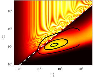
Energy contained in the principal response mode relative to the total response, $\unicode[STIX]{x1D70E}_{1}^{2}/(\sum _{j}\unicode[STIX]{x1D70E}_{j}^{2})$, for different streamwise and spanwise wavelengths for the (a,c) incompressible and (b,d) compressible ($M_{\infty }=4$) turbulent boundary layers at (a,b) $x_{2}^{+}=15$ and (c,d) $x_{2}/\unicode[STIX]{x1D6FF}=0.2$. The contours are 10 %, 50 % and 90 % of the maximum energy of the premultiplied energy spectra for channel flow at $Re_{\unicode[STIX]{x1D70F}}\approx 550$ (Del Alamo et al. Reference Del Alamo, Jiménez, Zandonade and Moser2004) at the corresponding wall-normal locations. The white dashed line indicates the relative Mach number of unity, $\overline{M}_{\infty }=1$.

Figure 2.

Energy contained in the principal response mode relative to the total response, $\unicode[STIX]{x1D70E}_{1}^{2}/(\sum _{j}\unicode[STIX]{x1D70E}_{j}^{2})$, for different streamwise and spanwise wavelengths and wave speeds for the (a) incompressible, (b) $M_{\infty }=2$, $Re_{\unicode[STIX]{x1D70F}}=450$, (c) $M_{\infty }=3$ and (d) $M_{\infty }=4$ cases. The contour surface is $\unicode[STIX]{x1D70E}_{1}^{2}/(\sum _{j}\unicode[STIX]{x1D70E}_{j}^{2})=0.75$ coloured by wall-normal distance from the wall.

We first examine the energy contained in the principal response mode. The energy contribution of $\unicode[STIX]{x1D74D}_{k}$ to the total response subject to broadband forcing in the wall-normal direction can be quantified by $\unicode[STIX]{x1D70E}_{k}^{2}/(\sum _{j}\unicode[STIX]{x1D70E}_{j}^{2})$. Figure 1 shows the principal energy contribution from the principal response mode $\unicode[STIX]{x1D74D}_{1}$ for the incompressible case and the $M_{\infty }=4$ case at two wall-normal locations $x_{2}^{+}=15$ and $x_{2}/\unicode[STIX]{x1D6FF}=0.2$, where the superscript $+$ denotes wall units defined in terms of $\bar{\unicode[STIX]{x1D70C}}$ and $\unicode[STIX]{x1D707}$ at the wall and the friction velocity $u_{\unicode[STIX]{x1D70F}}$.

The results from the incompressible and compressible turbulent boundary layers show similarities in the region where the principal energy contribution of the incompressible boundary layer is concentrated, i.e. where the low-rank approximation is valid for the incompressible regime. This region coincides with the most energetic wavenumbers from DNS of incompressible channel flows identified by the premultiplied energy spectra given by the contour lines in the figure. While the premultiplied energy spectra shown here are from a DNS of channel flow, many studies in the past show similarities in higher-order streamwise statistics for internal and external flows (Mochizuki & Nieuwstadt Reference Mochizuki and Nieuwstadt1996; Metzger & Klewicki Reference Metzger and Klewicki2001; Del Alamo et al. Reference Del Alamo, Jiménez, Zandonade and Moser2004; Jiménez & Hoyas Reference Jiménez and Hoyas2008; Monty et al. Reference Monty, Hutchins, Ng, Marusic and Chong2009), especially in the near-wall region. Moreover, while comparisons between energy spectra of incompressible and compressible boundary layers are not available, first-order statistics of the two cases for adiabatic wall boundary conditions are known to collapse given a correct velocity transformation (Pirozzoli & Bernardini Reference Pirozzoli and Bernardini2011), making the comparison still meaningful. While data such as two-dimensional energy spectra at various wall-normal heights for incompressible and compressible boundary layers are not readily obtainable, access to such data could facilitate the analysis in the future.

The most notable difference between the incompressible and compressible results is the triangular region marked by free-stream relative Mach number (Mack Reference Mack1984), $\overline{M}_{\infty }=\overline{M}(x_{2}\rightarrow \infty )$, greater than unity (figure 1b). The relative Mach number, defined as

(3.1)

$$\begin{eqnarray}\overline{M}(x_{2})=\frac{(\unicode[STIX]{x1D705}_{1}\bar{u}_{1}(x_{2})-\unicode[STIX]{x1D714})M_{\infty }}{(\unicode[STIX]{x1D705}_{1}^{2}+\unicode[STIX]{x1D705}_{3}^{2})^{1/2}\bar{T}(x_{2})^{1/2}},\end{eqnarray}$$

can be understood as the local Mach number of the mean flow in the direction of the wavenumber vector, $[\unicode[STIX]{x1D705}_{1},\unicode[STIX]{x1D705}_{3}]^{\intercal }$, relative to the wave speed at a given wall-normal location $x_{2}$. A three-dimensional depiction of the principal energy contribution as a function of streamwise and spanwise wavenumbers and wave speeds is given in figure 2 for the incompressible case and the compressible case at three different Mach numbers. It is clear that the region with $\overline{M}_{\infty }>1$, i.e. the relatively supersonic region, increases with Mach number and grows from the wall towards the free stream. In linear stability theory, $\overline{M}_{\infty }$ has been used to classify disturbances as subsonic, sonic or supersonic (Mack Reference Mack1984; Schmid & Henningson Reference Schmid and Henningson2000). Moreover, it has been shown that if $\overline{M}_{\infty }>1$, a compressible boundary layer is unstable to inviscid waves regardless of any other feature of the velocity and temperature profiles (Mack Reference Mack1984). Considering that the family of modes with $\overline{M}_{\infty }>1$ does not have any counterpart in incompressible boundary layers, it is expected that the largest deviation between the compressible and incompressible boundary layers occurs in this regime. In particular, the irregular low-rank behaviour present in the relatively supersonic region in figures 1(b) and 2(b–d) is due to the discrete acoustic eigenmodes of the system approaching the wave speed $c$ (appendix A) thus giving resonant amplification of the resolvent operator (Dawson & McKeon Reference Dawson and McKeon2019). This is a consequence of discretisation, and in the continuous case, this resonant amplification effect will be present everywhere in the relatively supersonic region. The extent of the relatively supersonic region, where the incompressible and compressible boundary layers show a significant difference, increases with increasing Mach number, and may be an indicator of why Morkovin’s hypothesis fails for high Mach numbers.

The second, although less significant, difference can be seen for the two spectra at $x_{2}/\unicode[STIX]{x1D6FF}=0.2$ shown in figure 1(c,d), where the region of high energy contribution covers a much wider range of wall-parallel wavelengths for the $M_{\infty }=4$ case, with the ‘nose’ of the spectrum located at a smaller $(\unicode[STIX]{x1D706}_{1}/\unicode[STIX]{x1D6FF},\unicode[STIX]{x1D706}_{3}/\unicode[STIX]{x1D6FF})$.

The first observation regarding the relative Mach number of unity can be explained by the formation of Mach waves in the relatively supersonic region. The second can be comprehended in terms of the correct scaling required for the compressible boundary layer. These main two observations will be discussed in the remainder of this section.

3.1 Relatively supersonic region and Mach waves

As displayed by the energy contribution in figure 1, the resolvent operator is shown to exhibit low-rank behaviour for the supersonic turbulent boundary layer as well as for the incompressible case. Moarref et al. (Reference Moarref, Sharma, Tropp and McKeon2013) showed that significant understanding of the scaling of wall turbulence can be obtained by using the simple rank-1 model. Here, we employ the same rank-1 model by only keeping the most energetic forcing and response directions corresponding to $\unicode[STIX]{x1D70E}_{1}$ and compute the premultiplied one-dimensional energy density of the principal response of $\unicode[STIX]{x1D643}$ defined as

(3.2)

$$\begin{eqnarray}E_{qq}(x_{2},\unicode[STIX]{x1D714})=\mathop{\sum }_{i=1}^{5}\frac{\displaystyle \iint \unicode[STIX]{x1D705}_{1}^{2}\unicode[STIX]{x1D705}_{3}\left[\unicode[STIX]{x1D70E}_{1}(\unicode[STIX]{x1D705}_{1},\unicode[STIX]{x1D705}_{3},\unicode[STIX]{x1D714})|(q_{i})_{1}|(\unicode[STIX]{x1D705}_{1},x_{2},\unicode[STIX]{x1D705}_{3},\unicode[STIX]{x1D714})\right]^{2}\,\text{d}\log \unicode[STIX]{x1D705}_{1}\,\text{d}\log \unicode[STIX]{x1D705}_{3}}{\displaystyle \max \iint \unicode[STIX]{x1D705}_{1}^{2}\unicode[STIX]{x1D705}_{3}\unicode[STIX]{x1D70E}_{1}(\unicode[STIX]{x1D705}_{1},\unicode[STIX]{x1D705}_{3},\unicode[STIX]{x1D714})^{2}\,\text{d}\log \unicode[STIX]{x1D705}_{1}\,\text{d}\log \unicode[STIX]{x1D705}_{3}}.\end{eqnarray}$$

Figure 3.

Premultiplied one-dimensional energy density $E_{qq}$ for the (a) incompressible and (b) compressible ($M_{\infty }=2,Re_{\unicode[STIX]{x1D70F}}=450$) cases, and the energy density for the compressible case conditionally sampled to (c) $\overline{M}_{\infty }<1$ and (d) $\overline{M}_{\infty }>1$. The turbulent mean velocity profile, $\bar{u}_{1}$ (——) and the relative sonic line $\bar{c}$ (- - -) are shown for reference. Colours are in logarithmic scale.

In figure 3(a,b), we plot the energy density as a function of wave speed $c$ and $x_{2}$ for both the incompressible and supersonic ($M_{\infty }=2$, $Re_{\unicode[STIX]{x1D70F}}=450$) turbulent boundary layers. Unlike the incompressible case, where the energy density is localised around the mean velocity profile (solid line), the compressible case shows a second region which is displaced from the mean velocity. The overlaid relative sonic line (dashed line), where the velocity profile corresponds to relative streamwise Mach number of unity at each wall-normal location, shows that the displacement of the areas of high energy density is indicative of Mach waves. The relative sonic line $\bar{c}$ is given by solving

(3.3)

$$\begin{eqnarray}\overline{M}=\frac{(\unicode[STIX]{x1D705}_{1}\bar{u}_{1}-\unicode[STIX]{x1D705}_{1}\bar{c})M_{\infty }}{\left(\unicode[STIX]{x1D705}_{1}^{2}+\unicode[STIX]{x1D705}_{3}^{2}\right)^{1/2}\bar{T}^{1/2}}=1\end{eqnarray}$$

at each $x_{2}$ for $\unicode[STIX]{x1D705}_{3}=0$, i.e. $\bar{c}=\bar{u}_{1}-\bar{T}^{1/2}/M_{\infty }$, and indicates the minimum streamwise velocity at each $x_{2}$ where a relatively supersonic region exists. From conditionally sampling the energy intensity for $\overline{M}_{\infty }<1$ or $\overline{M}_{\infty }>1$ by evaluating (3.2) with the integrand of the numerator multiplied by an indicator function for each case (as shown in figure 3c,d), the two phenomena can clearly be separated, and the second region of high energy density can be attributed entirely to the relatively supersonic region of $\overline{M}_{\infty }>1$ and the existence of modes resembling Mach waves.

In figure 4, we plot a few of the principal streamwise velocity response modes $(u_{1})_{1}$ for both the incompressible and compressible $(M_{\infty }=2,Re_{\unicode[STIX]{x1D70F}}=450)$ cases at $(\unicode[STIX]{x1D706}_{1}/\unicode[STIX]{x1D6FF},\unicode[STIX]{x1D706}_{3}/\unicode[STIX]{x1D6FF})=(0.01,10)$, which lie within the region $\overline{M}_{\infty }>1$ for the compressible case for a variety of wave speeds. Note that the modes under consideration are essentially two-dimensional, as we need $\unicode[STIX]{x1D706}_{1}\ll \unicode[STIX]{x1D706}_{3}$ in order for the relatively supersonic region to exist for a wide range of wall-normal locations. This aspect ratio has not been studied in the past in the context of unforced turbulent boundary layers and the mode shapes that occur here are different from the nominal three-dimensional case.

Examining the principal response modes, we see the modes for the incompressible case (figure 4a) are centred at the critical layer $x_{2}^{c}$, where $\bar{u}_{1}(x_{2}^{c})=c$, but the modes corresponding to $\overline{M}_{\infty }>1$ for the compressible case (figure 4b) are centred at the sonic layer, $x_{2}^{s}$, where $\overline{M}(x_{2}^{s})=1$. Although not shown, the other velocity, density and temperature modes, and consequently the pressure modes, are also centred in the sonic layer. These response modes are consistent with Mach waves that propagate towards the free stream and the concept of eddy shocklets (Phillips Reference Phillips1960; Ffowcs Williams & Maidanik Reference Ffowcs Williams and Maidanik1965), where the instantaneous supersonic events cause local shock-like structures in the boundary layer. However, the analysis of the formation of eddy shocklets from superimposed Mach waves requires additional knowledge of phase for each wave parameter and is not considered here.

Figure 4.

The response modes $(u_{1})_{1}$ for the (a) incompressible and (b) supersonic ($M_{\infty }=2,Re_{\unicode[STIX]{x1D70F}}=450$) turbulent boundary layers with $\unicode[STIX]{x1D706}_{1}/\unicode[STIX]{x1D6FF}=0.01$, $\unicode[STIX]{x1D706}_{3}/\unicode[STIX]{x1D6FF}=10$ and $c=0.14$ (blue), $0.26$ (red), $0.38$ (green). Reference lines are the wall-normal locations of the critical layer, $x_{2}=x_{2}^{c}$ (- - -), and the sonic layer, $x_{2}=x_{2}^{s}$ (– ⋅ – ⋅ –).

3.2 Relatively subsonic region and universality of resolvent modes

In order for the resolvent modes to exhibit universal behaviour for different $Re_{\unicode[STIX]{x1D70F}}$, the modes must have a narrow footprint such that the support of the modes in the wall-normal direction is localised. This is because, otherwise, resolvent modes are affected by the mean velocity at various wall-normal locations that scale differently with $Re_{\unicode[STIX]{x1D70F}}$ (Moarref et al. Reference Moarref, Sharma, Tropp and McKeon2013). Moreover, the necessary condition for the existence of geometrically self-similar resolvent modes is the presence of a logarithmic region in the turbulent mean velocity profile.

Figure 5.

(a) Turbulent mean streamwise velocity profile $\bar{u}_{1}^{+}(x_{2}^{+})$, (b) the transformed velocity profile $\bar{u}_{1}^{\ast }(x_{2}^{\ast })$ given by (3.5), (c) the defect velocity $\bar{u}_{1,\infty }^{+}-\bar{u}_{1}^{+}(x_{2}/\unicode[STIX]{x1D6FF})$ with respect to the free stream and (d) the transformed defect velocity $\bar{u}_{1,\infty }^{\star }-\bar{u}_{1}^{\star }(x_{2}/\unicode[STIX]{x1D6FF})$ given by (3.7). Lines indicate $M_{\infty }=0$ (- - -), $M_{\infty }=2,Re_{\unicode[STIX]{x1D70F}}=450$ (

, blue),

$M_{\infty }=2,Re_{\unicode[STIX]{x1D70F}}=900$ (

, blue),

$M_{\infty }=3$ (

, red) and

$M_{\infty }=4$ (

, green).

In order for the resolvent modes to be universal for the supersonic boundary layer, not only do the modes have to be localised in $x_{2}$, but the mean velocity profile must have a scaling law similar to that of the incompressible case such that different regions of the mean profiles collapse for various $M_{\infty }$ and $Re_{\unicode[STIX]{x1D70F}}$. In compressible flows, viscous heating causes non-uniform mean density and viscosity, which results in a mean velocity profile that no longer satisfies the scaling of its incompressible counterpart. Many attempts have been made to recover the scalings in this regime (Wilson Reference Wilson1950; Van Driest Reference Van Driest1951; Coles Reference Coles1964; Zhang et al. Reference Zhang, Bi, Hussain, Li and She2012; Trettel & Larsson Reference Trettel and Larsson2016, among others), with particular emphasis on the logarithmic region. Most of these attempts have been made by seeking a transformation of $\bar{u}_{1}$ and $x_{2}$ such that the compressible velocity profile maps onto an equivalent incompressible profile. The most recent of these approaches given by Trettel & Larsson (Reference Trettel and Larsson2016) utilises a semi-local scaling in $x_{2}$ and an integrated stress-balance condition, which assumes that the sum of viscous and Reynolds stresses in both the raw and transformed states must be equal, for the scaling of $\bar{u}_{1}$ such that

(3.4)

$$\begin{eqnarray}\displaystyle & \displaystyle x_{2}^{\ast }=\frac{\bar{\unicode[STIX]{x1D70C}}\left(\unicode[STIX]{x1D70F}_{w}/\bar{\unicode[STIX]{x1D70C}}\right)^{1/2}x_{2}}{\bar{\unicode[STIX]{x1D707}}}, & \displaystyle\end{eqnarray}$$

(3.5)

$$\begin{eqnarray}\displaystyle & \displaystyle \bar{u}_{1}^{\ast }=\int _{0}^{\bar{u}_{1}^{+}}\left(\frac{\bar{\unicode[STIX]{x1D70C}}}{\bar{\unicode[STIX]{x1D70C}}_{w}}\right)^{1/2}\left(1+\frac{1}{2\bar{\unicode[STIX]{x1D70C}}}\frac{\text{d}\bar{\unicode[STIX]{x1D70C}}}{\text{d}x_{2}}x_{2}-\frac{1}{\bar{\unicode[STIX]{x1D707}}}\frac{\text{d}\bar{\unicode[STIX]{x1D707}}}{\text{d}x_{2}}x_{2}\right)\,\text{d}\bar{u}_{1}^{+}. & \displaystyle\end{eqnarray}$$

Here, the subscript $w$ indicates quantities evaluated at the wall, and $\unicode[STIX]{x1D70F}_{w}$ is the wall shear stress. The results of this transformation are illustrated in figure 5(a,b), and an improved collapse of the mean velocity profile in the inner and logarithmic regions for the various Mach numbers is achieved. The semi-local scaling $x_{2}^{\ast }$ used here was introduced by Lobb, Winkler & Persh (Reference Lobb, Winkler and Persh1955), revisited by Coleman, Kim & Moser (Reference Coleman, Kim and Moser1995) and Huang et al. (Reference Huang, Coleman and Bradshaw1995) and generalised by Trettel & Larsson (Reference Trettel and Larsson2016). This scaling gives rise to a semi-local Reynolds number (Cebeci & Bradshaw Reference Cebeci and Bradshaw2012; Patel et al. Reference Patel, Peeters, Boersma and Pecnik2015) at each wall-normal location

(3.6)

$$\begin{eqnarray}Re_{\unicode[STIX]{x1D70F}}^{\ast }(x_{2})=\frac{\bar{\unicode[STIX]{x1D70C}}(\unicode[STIX]{x1D70F}_{w}/\bar{\unicode[STIX]{x1D70C}})^{1/2}\unicode[STIX]{x1D6FF}}{\bar{\unicode[STIX]{x1D707}}}\end{eqnarray}$$

such that $x_{2}^{\ast }=(x_{2}/\unicode[STIX]{x1D6FF})Re_{\unicode[STIX]{x1D70F}}^{\ast }$. While the transformation proposed by Trettel & Larsson (Reference Trettel and Larsson2016) works well for the inner and logarithmic regions, the collapse is not as good for the outer region. We find that the best collapse for the outer region is achieved with the transformation

(3.7)

$$\begin{eqnarray}\bar{u}_{1}^{\star }=\bar{u}_{1}^{+}\left(\frac{\bar{\unicode[STIX]{x1D70C}}}{\bar{\unicode[STIX]{x1D70C}}_{w}}\right)^{1/2},\end{eqnarray}$$

which is equivalent to scaling the velocity with the semi-local $u_{\unicode[STIX]{x1D70F}}^{\ast }=\sqrt{\unicode[STIX]{x1D70F}_{w}/\bar{\unicode[STIX]{x1D70C}}}$ instead of $u_{\unicode[STIX]{x1D70F}}=\sqrt{\unicode[STIX]{x1D70F}_{w}/\bar{\unicode[STIX]{x1D70C}}_{w}}$, and the results are given in figure 5(c,d). A different transformation for the outer layer is expected since the transformation given in (3.5) is based on the idea that momentum conservation can be achieved by satisfying the stress-balance condition, which only holds in the inner layer of nearly parallel shear flow at reasonable turbulence Mach numbers. Note that despite the better scaling in the outer region, the collapse is not perfect, which is a known issue for low Reynolds number boundary layer flows. Still, a universal mean velocity profile for the inner, logarithmic and outer layers can be achieved by utilising the semi-local scaling.

Figure 6.

Energy contained in the principal response mode relative to the total response for different streamwise and spanwise wavelengths for the (a) incompressible ($Re_{\unicode[STIX]{x1D70F}}=1040$) and (b) compressible ($M_{\infty }=4$, $Re_{\unicode[STIX]{x1D70F}}^{\ast }=1020$) turbulent boundary layer at $x_{2}/\unicode[STIX]{x1D6FF}=0.2$. The contours are 10 %, 50 % and 90 % of the maximum energy of the premultiplied energy spectra for channel flow at $Re_{\unicode[STIX]{x1D70F}}\approx 950$ (Del Alamo et al. Reference Del Alamo, Jiménez, Zandonade and Moser2004) at the corresponding wall-normal location.

Given that the transformation of the turbulent supersonic mean velocity profile in (3.4)–(3.7) produces a reasonable match to the incompressible profile in the inner, outer and logarithmic regions, the relatively subsonic ($\overline{M}_{\infty }<1$) resolvent modes are expected to have a universal behaviour in both Reynolds and Mach number, as the one-dimensional energy density conditioned to $\overline{M}_{\infty }<1$ in figure 3(c) shows a localisation with respect to $x_{2}$. Moreover, the existence of a logarithmic region in the transformed mean streamwise velocity profile satisfies the necessary condition for the geometrically self-similar modes to be present. Due to the transformation in both $\bar{u}_{1}$ and $x_{2}$, the scaling of the resolvent modes should be with respect to the semi-local variables, $x_{2}^{\ast }$ and $Re_{\unicode[STIX]{x1D70F}}^{\ast }$. The detailed scaling laws for response modes of the inner, outer and logarithmic regions are given in § 4.1.

The semi-local scaling also explains the discrepancy between the principal energy contribution in the incompressible boundary layer (figure 1c) and the supersonic one (figure 1d). For the supersonic case of $M_{\infty }=4$, the semi-local Reynolds number at $x_{2}/\unicode[STIX]{x1D6FF}=0.2$ is $Re_{\unicode[STIX]{x1D70F}}^{\ast }=1020$, which is significantly larger than the Reynolds number of the incompressible case ($Re_{\unicode[STIX]{x1D70F}}=450$). In figure 6, we instead compare against the results from the incompressible turbulent boundary at $Re_{\unicode[STIX]{x1D70F}}=1040$ with the mean velocity profile from Schlatter & Örlü (Reference Schlatter and Örlü2010) and the premultiplied energy spectra from turbulent channel flow at $Re_{\unicode[STIX]{x1D70F}}=950$ (Del Alamo et al. Reference Del Alamo, Jiménez, Zandonade and Moser2004), which show a better qualitative comparison between the two principal energy contribution spectra than the comparison given in figure 1.

Figure 7.

Semi-local friction Reynolds number $Re_{\unicode[STIX]{x1D70F}}^{\ast }$ as a function of $x_{2}$ for $M_{\infty }=2,Re_{\unicode[STIX]{x1D70F}}=450$ (

, blue),

$M_{\infty }=2,Re_{\unicode[STIX]{x1D70F}}=900$ (

, blue),

$M_{\infty }=3$ (

, red) and

$M_{\infty }=4$ (

, green).

4 Scaling of the principal singular value and resolvent modes

4.1 Scaling of the principal response mode

As discussed in § 3.2, the mean streamwise velocity profile with the semi-local scaling collapses to the incompressible boundary layer profile. This implies that the same scaling used in Moarref et al. (Reference Moarref, Sharma, Tropp and McKeon2013) for the incompressible channel flow can be extended to the compressible boundary layer by using the length scale $x_{2}^{\ast }$ and Reynolds number $Re_{\unicode[STIX]{x1D70F}}^{\ast }$.

Note that $Re_{\unicode[STIX]{x1D70F}}^{\ast }$ depends on Mach number through the variation in density and temperature (see figure 7). For an adiabatic wall, the mean temperature profile is given by

(4.1)

$$\begin{eqnarray}\frac{\bar{T}}{\bar{T}_{\infty }}=1+r\frac{\unicode[STIX]{x1D6FE}-1}{2}M_{\infty }^{2}\left[1-\left(\frac{\bar{u}_{1}}{\bar{u}_{1,\infty }}\right)^{2}\right],\end{eqnarray}$$

where $r=Pr^{1/3}$ is the recovery factor (Walz Reference Walz1969). Given the definition of the semi-local Reynolds number (3.6) and the mean equation of state $\bar{p}=\bar{\unicode[STIX]{x1D70C}}\bar{T}=1$, we have

(4.2)

$$\begin{eqnarray}Re_{\unicode[STIX]{x1D70F}}^{\ast }=Re_{\unicode[STIX]{x1D70F}}\frac{\bar{\unicode[STIX]{x1D707}}/\bar{\unicode[STIX]{x1D707}}_{w}}{\sqrt{\bar{\unicode[STIX]{x1D70C}}/\bar{\unicode[STIX]{x1D70C}}_{w}}}=Re_{\unicode[STIX]{x1D70F}}\frac{(\bar{T}/\bar{T}_{w})^{3/2}+C_{w}}{(\bar{T}/\bar{T}_{w})^{3/2}(1+C_{w})},\end{eqnarray}$$

where $C_{w}=S/T_{w}$. When $x_{2}=0$, we have that $Re_{\unicode[STIX]{x1D70F}}^{\ast }=Re_{\unicode[STIX]{x1D70F}}$ as expected. In the limit $x_{2}\rightarrow \infty$, $\bar{T}/\bar{T}_{w}=1/(1+r(\unicode[STIX]{x1D6FE}-1)M_{\infty }^{2}/2)$ and we have

(4.3)

$$\begin{eqnarray}Re_{\unicode[STIX]{x1D70F}}^{\ast }(x_{2}\rightarrow \infty )=Re_{\unicode[STIX]{x1D70F}}\frac{1+C_{w}(1+r(\unicode[STIX]{x1D6FE}-1)M_{\infty }^{2}/2)^{3/2}}{1+C_{w}},\end{eqnarray}$$

giving approximately a $M_{\infty }^{3}$ dependence for high Mach numbers.

Table 2.

Expected length scales for the universal modes of the resolvent operator for the turbulent boundary layer.

In order for a fair comparison between the incompressible and compressible response modes to be made, the compressible velocity response modes must be normalised by the kinetic energy content in the response modes due to the orthonormality constraint of the singular vectors and the different norms used for the two cases. We define turbulent kinetic energy and turbulent thermodynamic energy as

(4.4a,b)

$$\begin{eqnarray}E_{K}=(\boldsymbol{q},\boldsymbol{q})_{K}=\int _{0}^{\infty }\bar{\unicode[STIX]{x1D70C}}u_{i}^{\dagger }u_{i}\,\text{d}x_{2},\quad E_{T}=\int _{0}^{\infty }\frac{1}{\unicode[STIX]{x1D6FE}M_{\infty }^{2}}\left(\frac{\unicode[STIX]{x1D70C}^{\dagger }\unicode[STIX]{x1D70C}}{\bar{\unicode[STIX]{x1D70C}}^{2}}+\frac{T^{\dagger }T}{\bar{T}^{2}}\right)\,\text{d}x_{2},\end{eqnarray}$$

respectively. We normalise the velocity, density and temperature modes such that

(4.5a-c)

$$\begin{eqnarray}\widetilde{(u_{i})}_{1}=\frac{\bar{\unicode[STIX]{x1D70C}}^{1/2}(u_{i})_{1}}{\sqrt{E_{K}}},\quad \widetilde{(\unicode[STIX]{x1D70C})}_{1}=\frac{(\unicode[STIX]{x1D70C})_{1}/(\unicode[STIX]{x1D6FE}M_{\infty }^{2}\bar{\unicode[STIX]{x1D70C}}^{2})^{1/2}}{\sqrt{E_{T}}},\quad \widetilde{(T)}_{1}=\frac{(T)_{1}/(\unicode[STIX]{x1D6FE}M_{\infty }^{2}\bar{T}^{2})^{1/2}}{\sqrt{E_{T}}}.\end{eqnarray}$$

The relationship between $E_{K}$ and $E_{T}$ is discussed later in § 4.3. The proposed scaling of the resolvent for the different classes of the compressible boundary layer is summarised in table 2. Note that the combined scaling of the normalised response modes, the singular values and the ratio of $E_{K}$ to $E_{T}$ is of importance when examining the response mode of the resolvent operator.

4.1.1 Outer region

Figure 8.

Normalised and scaled response modes in the outer region for streamwise velocity (a) $\widetilde{(u_{1})}_{1}^{out,+}$ and (b) $\widetilde{(u_{1})}_{1}^{out,\ast }$, density (c) $\widetilde{(\unicode[STIX]{x1D70C})}_{1}^{out,+}$ and (d) $\widetilde{(\unicode[STIX]{x1D70C})}_{1}^{out,\ast }$ and temperature (e) $\widetilde{(T)}_{1}^{out,+}$ and (f) $\widetilde{(T)}_{1}^{out,\ast }$. Lines indicate $M_{\infty }=0$ (- - -), $M_{\infty }=2,Re_{\unicode[STIX]{x1D70F}}=450$ (

, blue),

$M_{\infty }=2,Re_{\unicode[STIX]{x1D70F}}=900$ (

, blue),

$M_{\infty }=3$ (

, red) and

$M_{\infty }=4$ (

, green).

Because the difference between $Re_{\unicode[STIX]{x1D70F}}$ and $Re_{\unicode[STIX]{x1D70F}}^{\ast }$ grows as $x_{2}$ increases (see figure 7), the difference between the two scalings is expected to be most pronounced in the outer region, defined as $(\bar{u}_{1,\infty }^{\star }-\bar{u}_{1}^{\star })\lesssim 6$ with $\unicode[STIX]{x1D705}_{3}/\unicode[STIX]{x1D705}_{1}\gtrsim \unicode[STIX]{x1D716}Re_{\unicode[STIX]{x1D70F}}^{\ast }/Re_{\unicode[STIX]{x1D70F},min}^{\ast }$, $\unicode[STIX]{x1D716}^{2}\approx 10$ (see appendix B and Moarref et al. Reference Moarref, Sharma, Tropp and McKeon2013, for details). In this region, the $x_{2}$ dependent coefficients of $\unicode[STIX]{x1D643}$ such as $\bar{u}_{1}-c$ (and $\bar{T}$ and $\bar{\unicode[STIX]{x1D70C}}$) are independent of $Re_{\unicode[STIX]{x1D70F}}$. And in the incompressible case, the balance between the viscous dissipation term and the mean advection term in the resolvent requires scaling of the spanwise coordinate in $\unicode[STIX]{x1D6FF}$ and the streamwise coordinate with $\unicode[STIX]{x1D6FF}^{+}$ (Moarref et al. Reference Moarref, Sharma, Tropp and McKeon2013). Thus, the universal modes in the outer region for the incompressible case are given by the wave parameters

(4.6)

$$\begin{eqnarray}(q_{i})_{1}^{out,+}=(q_{i})_{1}\left(\unicode[STIX]{x1D705}_{1}=\unicode[STIX]{x1D705}_{1}^{ref}\frac{Re_{\unicode[STIX]{x1D70F}}^{ref}}{Re_{\unicode[STIX]{x1D70F}}},\unicode[STIX]{x1D705}_{3}=\unicode[STIX]{x1D705}_{3}^{ref},c=c^{ref}\right)\end{eqnarray}$$

in wall units. Using semi-local variables, we expect the wave parameters for the compressible case to be

(4.7)

$$\begin{eqnarray}(q_{i})_{1}^{out,\ast }=(q_{i})_{1}\left(\unicode[STIX]{x1D705}_{1}=\unicode[STIX]{x1D705}_{1}^{ref}\frac{Re_{\unicode[STIX]{x1D70F}}^{ref}}{Re_{\unicode[STIX]{x1D70F}}^{\ast }},\unicode[STIX]{x1D705}_{3}=\unicode[STIX]{x1D705}_{3}^{ref},c=c^{ref}\right).\end{eqnarray}$$

Due to the scaling of the wall-normal distance in outer units as well as the orthonormality condition for the response modes, i.e. $((\boldsymbol{q})_{1},(\boldsymbol{q})_{1})_{E}=1$, the mode height is expected to scale in outer units. In figure 8, we plot the normalised and scaled principal streamwise velocity, density and temperature response modes, with the reference parameters $Re_{\unicode[STIX]{x1D70F}}^{ref}=445.5$, $\unicode[STIX]{x1D705}_{1}^{ref}\unicode[STIX]{x1D6FF}=1$, $\unicode[STIX]{x1D705}_{3}^{ref}\unicode[STIX]{x1D6FF}=10$ and $c^{ref}/\bar{u}_{1,\infty }=0.98$. These reference parameters correspond to the very large scale structures for the incompressible case. The collapse among different Mach numbers is excellent for the semi-local scaling, and the streamwise velocity modes for the supersonic cases are indistinguishable from the incompressible response modes. By comparison, the modes do not collapse for various Mach numbers when scaled in wall units, with the modes becoming narrower in $x_{2}$ and the peak of the modes shifting closer to the wall with increasing Mach number. Although not shown, the wall-normal velocity response modes exhibit a similar collapse when scaled with $Re_{\unicode[STIX]{x1D70F}}^{\ast }$ as opposed to $Re_{\unicode[STIX]{x1D70F}}$, the proposed scaling in Sharma, Moarref & McKeon (Reference Sharma, Moarref and McKeon2017) for the incompressible case. The collapse is not as good for the spanwise velocity response modes (not shown), although the mode shape is still very similar among different Mach numbers. Furthermore, the mode shapes are comparable for the streamwise velocity, density and temperature. The resemblance of the density and temperature response modes can be explained by the fact that from the equation of state, the two are linked with the pressure fluctuations. Moreover, the similarity between the streamwise velocity and thermal modes reinforces the strong Reynolds analogy, which links the transport of momentum and heat transfer, and it can be concluded that the velocity and temperature profiles are correlated.

4.1.2 Inner region

In the case of the inner region, the deviation of $Re_{\unicode[STIX]{x1D70F}}$ and $Re_{\unicode[STIX]{x1D70F}}^{\ast }$ is not as significant, as can be seen in figure 7, leading to a similar result for both the wall-unit scaling and the semi-local scaling. For the universal modes in the inner region, where the streamwise and spanwise coordinates are given in inner units, we expect the universal wave parameters to be

(4.8)

$$\begin{eqnarray}(q_{i})_{1}^{in,\ast }=(q_{i})_{1}\left(\unicode[STIX]{x1D705}_{1}=\unicode[STIX]{x1D705}_{1}^{ref}\frac{Re_{\unicode[STIX]{x1D70F}}^{\ast }}{Re_{\unicode[STIX]{x1D70F}}^{ref}},\unicode[STIX]{x1D705}_{3}=\unicode[STIX]{x1D705}_{3}^{ref}\frac{Re_{\unicode[STIX]{x1D70F}}^{\ast }}{Re_{\unicode[STIX]{x1D70F}}^{ref}},c^{\ast }=c^{ref\ast }\right)\end{eqnarray}$$

for $x_{2}^{ref\ast }<30$ and $\unicode[STIX]{x1D705}_{3}/\unicode[STIX]{x1D705}_{1}\gtrsim \unicode[STIX]{x1D716}$, and analogously defined for $(q_{i})_{1}^{in,+}$. In figure 9, we plot the normalised and scaled principal streamwise velocity, density and temperature response modes for reference Reynolds number, $Re_{\unicode[STIX]{x1D70F}}^{ref}=445.5$ and wave parameters $\unicode[STIX]{x1D705}_{1}^{ref}\unicode[STIX]{x1D6FF}=1$, $\unicode[STIX]{x1D705}_{3}^{ref}\unicode[STIX]{x1D6FF}=10$ and $x_{2}^{ref\ast }=10$ (and $x_{2}^{ref+}=10$ for comparison). Here, the scaling of the wall-normal distance is in semi-local (or wall) units. Thus, the orthonormality condition for the velocity and thermodynamic modes requires that the response mode height is expected to scale as $1/\sqrt{Re_{\unicode[STIX]{x1D70F}}^{\ast }}$ (or $1/\sqrt{Re_{\unicode[STIX]{x1D70F}}}$). Again, the collapse of the response modes among different Mach numbers is good for both cases, and the streamwise velocity response modes also collapse with the incompressible case. The wall-normal and spanwise velocity response modes also collapse for the various Mach numbers to the incompressible case but are not shown for brevity. The mode shapes for density and temperature are almost identical for the same reasons discussed above. The temperature and density modes scaled in wall units are not shown, but they are almost identical to the ones given in semi-local units.

Figure 9.

Normalised and scaled response modes in the inner region for streamwise velocity (a) $\widetilde{(u_{1})}_{1}^{in,+}$ and (b) $\widetilde{(u_{1})}_{1}^{in,\ast }$, (c) density, $\widetilde{(\unicode[STIX]{x1D70C})}_{1}^{in,\ast }$ and (d) temperature $\widetilde{(T)}_{1}^{in,\ast }$ scaled by either $Re_{\unicode[STIX]{x1D70F}}^{-1/2}$ (a) or $Re_{\unicode[STIX]{x1D70F}}^{\ast -1/2}$ (b,c,d) for reference parameters $Re_{\unicode[STIX]{x1D70F}}^{ref}=445.5$, $\unicode[STIX]{x1D705}_{1}^{ref}\unicode[STIX]{x1D6FF}=1$, $\unicode[STIX]{x1D705}_{3}^{ref}\unicode[STIX]{x1D6FF}=10$ and $x_{2}^{\ast /+,\text{ref}}=10$. Lines indicate $M_{\infty }=0$ (- - -), $M_{\infty }=2,Re_{\unicode[STIX]{x1D70F}}=450$ (

, blue),

$M_{\infty }=2,Re_{\unicode[STIX]{x1D70F}}=900$ (

, blue),

$M_{\infty }=3$ (

, red) and

$M_{\infty }=4$ (

, green).

4.1.3 Logarithmic region

Figure 10.

Normalised and scaled response modes in the logarithmic region for streamwise velocity (a) $\widetilde{(u_{1})}_{1}^{log,+}$ and (b) $\widetilde{(u_{1})}_{1}^{log,\ast }$, (c) density $\widetilde{(\unicode[STIX]{x1D70C})}_{1}^{log,\ast }$ and (d) temperature $\widetilde{(T)}_{1}^{log,\ast }$ scaled by $\sqrt{x_{2}^{c}}$. Lines indicate $M_{\infty }=0$ (- - -), $M_{\infty }=2,Re_{\unicode[STIX]{x1D70F}}=450$ (

, blue),

$M_{\infty }=2,Re_{\unicode[STIX]{x1D70F}}=900$ (

, blue),

$M_{\infty }=3$ (

, red) and

$M_{\infty }=4$ (

, green).

Finally, while the $Re_{\unicode[STIX]{x1D70F}}$ for the cases under consideration is too small for a clearly defined logarithmic region, we consider the self-similar response modes. The wave parameters in this region are given by

(4.9)

$$\begin{eqnarray}(q_{i})_{1}^{log,\ast }=(q_{i})_{1}\left(\unicode[STIX]{x1D705}_{1}=\unicode[STIX]{x1D705}_{1}^{ref}\frac{x_{2}^{ref}x_{2}^{ref\ast }}{x_{2}^{c}x_{2}^{c\ast }},\unicode[STIX]{x1D705}_{3}=\unicode[STIX]{x1D705}_{3}^{ref}\frac{x_{2}^{ref}}{x_{2}^{c}},c\right)\end{eqnarray}$$

for wave speeds $c$ in the logarithmic region ($30/Re_{\unicode[STIX]{x1D70F}}^{\ast }<x_{2}/\unicode[STIX]{x1D6FF}<0.15$) (Tennekes & Lumley Reference Tennekes and Lumley1972), where $x_{2}^{ref}$ denotes the critical layer for $c^{ref}$. The wave parameters in wall units are given analogously for $(q_{i})_{1}^{log,+}$. In figure 10, we plot the normalised and scaled principal streamwise velocity, density and temperature response modes for reference Reynolds number, $Re_{\unicode[STIX]{x1D70F}}^{ref}=445.5$, and reference wave parameters $\unicode[STIX]{x1D705}_{1}^{ref}\unicode[STIX]{x1D6FF}=1$, $\unicode[STIX]{x1D705}_{3}^{ref}\unicode[STIX]{x1D6FF}=10$ and $c^{ref}/\bar{u}_{1,\infty }=0.5$. The orthonormality condition for the velocity and thermodynamic quantities give the response mode height scaling of $\sqrt{x_{2}^{c}/\unicode[STIX]{x1D6FF}}$. Similar to the outer region, the semi-local scaling gives a better collapse among the supersonic response modes for various Mach numbers. While the agreement with the incompressible case is not perfect, some improvement is made from the use of the semi-local scale. As mentioned earlier, the $Re_{\unicode[STIX]{x1D70F}}$ for cases under consideration is too low for an actual logarithmic layer and a better collapse is expected for higher Reynolds numbers. Additionally, as in the case of the inner and outer region, the temperature and density modes are identical and are similar to the streamwise velocity mode shape as well.

4.2 Scaling of the principal singular values

Figure 11.

Principal singular value in the relatively subsonic region for (a) $c=\bar{u}_{1,\infty }(x_{2}^{\ast }=10)$ for the inner layer, (b) $c/\bar{u}_{1,\infty }=0.7$ for the logarithmic layer and (c) $c/\bar{u}_{1,\infty }=0.88$ for the outer layer. Contour lines are (a) $(10^{2},10^{4},10^{6},10^{8})/\sqrt{Re_{\unicode[STIX]{x1D70F}}^{\ast }Re_{\unicode[STIX]{x1D70F}}^{\star }}$, (b) $(10^{-3},10^{-1},10^{1},10^{3})\times x_{2}^{\ast }x_{2}^{\star }x_{2}/\unicode[STIX]{x1D6FF}$ and (c) $(10^{-7},10^{-4},10^{-1},10^{2})\times Re_{\unicode[STIX]{x1D70F}}^{\star }Re_{\unicode[STIX]{x1D70F}}^{\ast }$. Lines indicate $M_{\infty }=0$ (- - -), $M_{\infty }=2,Re_{\unicode[STIX]{x1D70F}}=450$ (

, blue),

$M_{\infty }=2,Re_{\unicode[STIX]{x1D70F}}=900$ (

, blue),

$M_{\infty }=3$ (

, red) and

$M_{\infty }=4$ (

, green). Arrows indicate direction of increasing

$\unicode[STIX]{x1D70E}_{1}$.

In addition to the universality and self-similarity of the response modes, the scaling of the principal singular values is also investigated. The expected scaling of the singular values for the incompressible case is given by $1/Re_{\unicode[STIX]{x1D70F}}$ in the inner region, $x_{2}^{+2}x_{2}/\unicode[STIX]{x1D6FF}$ in the logarithmic region and $Re_{\unicode[STIX]{x1D70F}}^{2}$ in the outer region (Moarref et al. Reference Moarref, Sharma, Tropp and McKeon2013; Sharma et al. Reference Sharma, Moarref and McKeon2017). The scaling of the principal singular values can be found by performing a scaling analysis on the resolvent operator $\unicode[STIX]{x1D643}$ by assessing the Reynolds number dependency of the terms in the linearised operator $\unicode[STIX]{x1D647}$ (see appendix B for details). The elements of the resolvent operator matrix, and thus the leading singular value, can be shown to follow $1/\sqrt{Re_{\unicode[STIX]{x1D70F}}^{\ast }Re_{\unicode[STIX]{x1D70F}}^{\star }}$ in the inner region, $x_{2}^{\star }x_{2}^{\ast }x_{2}/\unicode[STIX]{x1D6FF}$ in the logarithmic region and $Re_{\unicode[STIX]{x1D70F}}^{\ast }Re_{\unicode[STIX]{x1D70F}}^{\star }$ in the outer region, where $Re_{\unicode[STIX]{x1D70F}}^{\star }=\bar{\unicode[STIX]{x1D70C}}u_{\unicode[STIX]{x1D70F}}\unicode[STIX]{x1D6FF}/\bar{\unicode[STIX]{x1D707}}$ and $x_{2}^{\star }=Re_{\unicode[STIX]{x1D70F}}^{\star }x_{2}/\unicode[STIX]{x1D6FF}$. This is due to the presence of the factor $\bar{T}\bar{\unicode[STIX]{x1D707}}/Re$ (or equivalently $\bar{\unicode[STIX]{x1D707}}/(Re\bar{\unicode[STIX]{x1D70C}})$) in the governing equations combined with the semi-local scaling of $\unicode[STIX]{x1D705}_{1}$, $\unicode[STIX]{x1D705}_{3}$ and $x_{2}$. The proposed scaling for the principal singular values is given in figure 11. Note that this scaling will converge to the scaling given in Moarref et al. (Reference Moarref, Sharma, Tropp and McKeon2013) in the incompressible limit.

4.3 Scaling of the kinetic and thermodynamic energy ratio

Due to the orthonormality constraint of the resolvent modes, the comparison between the compressible and incompressible resolvent modes in the previous section was for normalised response modes $\widetilde{(q_{i})}_{1}$. However, it is equally important to assess the distribution of energy among the kinetic and thermodynamic variables for the supersonic cases.

Figure 12.

The spectra of the ratio of turbulent thermodynamic and kinetic energy, $E_{T}/E_{K}$ computed from the principal resolvent modes at (a) $x_{2}^{s}=15$, (b) $x_{2}/\unicode[STIX]{x1D6FF}=0.2$ and (c) $x_{2}/\unicode[STIX]{x1D6FF}=0.5$ for the $M_{\infty }=2$, $Re_{\unicode[STIX]{x1D70F}}=450$ case. The relative sonic line $\bar{c}$ (

) is shown for reference. (d) The values of

$E_{T}/E_{K}$ at the most energetic wave parameters as defined in (4.11) for the principal resolvent modes (

$\times$) and DNS (——) for

$M_{\infty }=2$,

$Re_{\unicode[STIX]{x1D70F}}=450$ (blue),

$M_{\infty }=3$ (red) and

$M_{\infty }=4$ (green).

In figure 12(a–c), we plot the spectra of the ratio of thermodynamic energy and kinetic energy $E_{T}/E_{K}$ for the resolvent modes for $M_{\infty }=2$ and $Re_{\unicode[STIX]{x1D70F}}=450$ for two different wall-normal heights. For the incompressible case, this ratio would be uniformly zero. Close to the wall, where a relatively supersonic region is present, the thermodynamic energy clearly dominates in the relatively supersonic region as expected. Further away from the wall at $x_{2}/\unicode[STIX]{x1D6FF}=0.2$ and $x_{2}/\unicode[STIX]{x1D6FF}=0.5$, the thermodynamic energy still dominates in a smaller region with $\unicode[STIX]{x1D706}_{3}>\unicode[STIX]{x1D706}_{1}$ with the strongest amplification centred around $\unicode[STIX]{x1D705}_{1}\unicode[STIX]{x1D6FF}\approx 0.5$. This may be explained by the observation from Pirozzoli & Bernardini (Reference Pirozzoli and Bernardini2011) that in this region, the thermal streaks are more elongated in the spanwise direction compared to the velocity streaks. It is also consistent with the observation that large-scale pressure-carrying eddies or wavepackets, which are correlated with thermodynamic fluctuations, are more coherent in the spanwise direction for both incompressible (Sillero, Jiménez & Moser Reference Sillero, Jiménez and Moser2014) and hypersonic (Duan, Choudhari & Zhang Reference Duan, Choudhari and Zhang2016) boundary layers.

We also plot the ratio of turbulent kinetic energy to the sum of the mean-square density and temperature fluctuations obtained from DNS (Bernardini & Pirozzoli Reference Bernardini and Pirozzoli2011; Pirozzoli & Bernardini Reference Pirozzoli and Bernardini2011) as a function of $x_{2}$ in figure 12(d). In particular, we plot

(4.10)

$$\begin{eqnarray}\left(\frac{E_{T}}{E_{K}}\right)^{DNS}=\unicode[STIX]{x1D6FE}M_{\infty }^{2}\frac{\bar{\unicode[STIX]{x1D70C}}u_{i,rms}u_{i,rms}/(\bar{u}_{j}\bar{u}_{j})}{\unicode[STIX]{x1D70C}_{rms}^{2}/\bar{\unicode[STIX]{x1D70C}}^{2}+T_{rms}^{2}/\bar{T}^{2}},\end{eqnarray}$$

where rms denotes the root-mean-squared fluctuations from DNS. For all wall-normal locations, the ratio increases with Mach number. Moreover, the ratio increases as a function of $x_{2}$ for a fixed Mach number. In order to compare the results from the resolvent modes to DNS, we define the energy ratio of the most energetic mode as

(4.11)

$$\begin{eqnarray}\left(\frac{E_{T}}{E_{K}}\right)^{res}=\frac{E_{T}}{E_{K}}\left(\text{arg}\,\text{max}_{\unicode[STIX]{x1D705}_{1},\unicode[STIX]{x1D705}_{3}}\,\unicode[STIX]{x1D6F7}_{u_{1}u_{1}}(\unicode[STIX]{x1D705}_{1},\unicode[STIX]{x1D705}_{3})\right),\end{eqnarray}$$

where $\unicode[STIX]{x1D6F7}_{u_{1}u_{1}}$ is the premultiplied streamwise energy spectrum for the channel flow at $Re_{\unicode[STIX]{x1D70F}}=550$ obtained a priori from Del Alamo et al. (Reference Del Alamo, Jiménez, Zandonade and Moser2004). The $(E_{T}/E_{K})^{res}$ given by these wave parameters is plotted in figure 12(d). The agreement between the ratio of kinetic and thermodynamic energy given by the most energetic principal response mode of the resolvent analysis and the DNS is excellent in the logarithmic region. While DNS data are used to identify the wave parameters of the most energetic mode, note that the spectra are for incompressible channel flow rather than the compressible turbulent boundary layer. The discrepancy in the outer region, especially for the higher Mach numbers, may be due to the fact that the difference in the spectra of the boundary layer and channel flow, which was used to choose the wave parameters for the most energetic modes, becomes more pronounced in this region. This may possibly be mitigated by utilising energy spectra from boundary layer simulations. In the inner region, the estimated energy ratio plateaus, deviating from the DNS profile. This could be due to the increased contributions from relatively supersonic region, which is more prevalent in the near-wall region (see figures 1 and 2). Additionally, it is shown in LeHew, Guala & McKeon (Reference LeHew, Guala and McKeon2011) that the energetic contribution of structures with convection velocities less than $10u_{\unicode[STIX]{x1D70F}}$ is negligible in real turbulent flows, which corresponds to the region where the mismatch is pronounced.

5 Conclusions

We have applied resolvent analysis for the compressible Navier–Stokes equations to a supersonic zero-pressure-gradient turbulent boundary layer. From the low-rank approximation formulated for individual wall-parallel wavenumbers and frequencies, we have identified two distinct regions in the wave parameter space: the relatively supersonic region and the relatively subsonic region.

In the relatively supersonic region, marked by relative Mach number greater than unity, we show that the resolvent modes are centred around the relative sonic line rather than the critical layer and that the majority of the energy is carried by the thermodynamic fluctuations. These response modes are consistent with acoustic Mach waves propagating towards the free stream and the idea of eddy shocklets, where the instantaneous supersonic events cause local shock-like structures in the boundary layer. Additionally, the modes in this region are also shown to follow a modal amplification mechanism. The range of wave parameters corresponding to the relatively supersonic region, where the compressibility effects are concentrated, grows with Mach number, which might be an indicator of why Morkovin’s hypothesis fails for high Mach numbers.

In the relatively subsonic region, we show that the principal response modes are localised around the critical layer corresponding to the mean velocity profile. Furthermore, with the semi-local scaling proposed by Trettel & Larsson (Reference Trettel and Larsson2016), the mean velocity profiles collapse for various Reynolds and Mach numbers. This provides the necessary condition for the resolvent modes to exhibit universality and geometrical self-similarity when scaled with the semi-local Reynolds number and wall-normal distance. We show that the principal response modes are indeed universal and self-similar and that they follow the same scaling laws as the incompressible boundary layer when normalised by the fluctuating kinetic energy. This validates the notion of Morkovin’s hypothesis for the relatively subsonic region on a mode-by-mode basis. Moreover, the velocity modes and the temperature and density modes are qualitatively similar, consistent with the strong Reynolds analogy. We also provide scaling laws for the amplification factor of the principal response mode.

Finally, we show that the energy distribution between the velocity fluctuations and the thermodynamic fluctuations can be predicted from the energy distribution of the most energetic response mode. Coupled with the universality and self-similarity of the resolvent modes in the relatively subsonic region, this has implications in modelling and prediction of high-speed turbulence. As in the incompressible case, the self-similar resolvent modes facilitate analytical developments in the logarithmic region of the boundary layer. Additionally, this allows prediction tools developed for resolvent analysis of incompressible fluids to be applied to supersonic boundary layers.

The results show that the main difference between the compressible Navier–Stokes equations and the incompressible equations are due to a different scaling law originating from density variations in the wall-normal direction and the acoustic contribution in the relatively supersonic region. The full nonlinear closure then propagates the deviation through triadic interactions, which results in variations in the mean velocity profile. Future efforts will be focused on studying the effect of the feedback loop by incorporating limited self-interactions to estimate the forcing term as in Rosenberg, Symon & McKeon (Reference Rosenberg, Symon and McKeon2019) for the incompressible Navier–Stokes equations. Also, further efforts are necessary to study the effects of higher Mach numbers and different wall boundary conditions such as cooled walls.

Acknowledgement

The authors acknowledge support from the Air Force Office of Scientific Research grant FA9550-16-1-0232. The authors also thank Dr A. Lozano-Durán and Dr M. Cho for their insightful comments on the manuscript.

Appendix A. Modal amplification mechanism in the relatively supersonic region

The spectrum of the linear operator $\unicode[STIX]{x1D647}$ is obtained from solving the eigenvalue problem $\unicode[STIX]{x1D647}\boldsymbol{q}=\text{i}\unicode[STIX]{x1D714}\boldsymbol{q}$. Here, we plot the results for the $M_{\infty }=4$ case in terms of the complex wave speed $c=\text{Re}(c)+\text{i}\text{Im}(c)$ in figure 13 for two different grid resolutions in $x_{2}$, $N_{2}=401$ and $N_{2}=801$. We also tested finite domain heights, compared to the semi-infinite domain, and the resulting spectra are robust to this change (not shown). We see that besides the discrete modes, the spectra consist of continuous branches that are represented as discrete points which either converge towards a vertical line, as expected for the viscous modes in both incompressible and compressible boundary layers, or form a horizontal line close to the real axis for the acoustic modes. For the spectrum of $(\unicode[STIX]{x1D705}_{1}\unicode[STIX]{x1D6FF},\unicode[STIX]{x1D705}_{3}\unicode[STIX]{x1D6FF})=(0.2,2)$, relative Mach number, $\overline{M}_{\infty }=0.39$, is subsonic, and thus relatively supersonic modes are absent in this case. However, the spectrum for $(\unicode[STIX]{x1D705}_{1}\unicode[STIX]{x1D6FF},\unicode[STIX]{x1D705}_{3}\unicode[STIX]{x1D6FF})=(1,2)$ (figure 13b), where the relatively supersonic region is present, shows an additional feature indicative of a continuous branch of ‘acoustic’ eigenmodes close to $\text{Im}(c)=0$. In the relatively supersonic region, the resolvent norm shows peaks in both the leading singular value and the energy contained in the principal resolvent mode due to spectral amplification, i.e. the resonant effects from the operator becoming close to normal as the wave speed approaches the discrete acoustic eigenvalues. This shows that the irregular patterns in figure 1(b) are the consequence of discretisation, and that the resonant effects will be universally present in the continuous case.

For a given wave speed $c$, we can plot the distance $d_{\unicode[STIX]{x1D6EC}}$, under the norm given in (2.13), from $\unicode[STIX]{x1D714}=c\unicode[STIX]{x1D705}_{1}$ to the closest discrete acoustic eigenvalue as a function of wavenumbers $\unicode[STIX]{x1D705}_{1}$ and $\unicode[STIX]{x1D705}_{3}$. In figure 14, the inverse of the minimum eigenvalue distance is shown to correlate well with the leading singular value, which leads to correlation with the principal energy contribution $\unicode[STIX]{x1D70E}_{1}^{2}/(\sum _{j}\unicode[STIX]{x1D70E}_{j}^{2})$. As mentioned before, this is due to the resonant amplification of the resolvent operator through modal amplification mechanisms. The change in the discrete location of the acoustic eigenvalues as a function of $\unicode[STIX]{x1D705}_{1}$ and $\unicode[STIX]{x1D705}_{3}$ explains the irregular patterns in figure 1(b) in the relatively supersonic region. However, the patterns are a purely numerical phenomenon and are indicative of the fact that the resolvent operator does not exist.

Figure 13.

Eigenvalues for the linearised operator $\unicode[STIX]{x1D647}$ for the compressible ($M_{\infty }=4$) turbulent boundary layer for wave parameters (a) $(\unicode[STIX]{x1D705}_{1}\unicode[STIX]{x1D6FF},\unicode[STIX]{x1D705}_{3}\unicode[STIX]{x1D6FF})=(0.2,2)$ and (b) $(\unicode[STIX]{x1D705}_{1}\unicode[STIX]{x1D6FF},\unicode[STIX]{x1D705}_{3}\unicode[STIX]{x1D6FF})=(1,2)$ for $N_{2}=401$ ($\times$) and $N_{2}=801$ (

Figure 14.

Inverse of the distance of the wave speed to the closest acoustic eigenvalue with $\text{Im}(c)=0$, $\unicode[STIX]{x1D705}_{1}/d_{\unicode[STIX]{x1D6EC}}$ (——), compared with the premultiplied principal singular value $\unicode[STIX]{x1D705}_{1}\unicode[STIX]{x1D6FF}\unicode[STIX]{x1D70E}_{1}$ (

) and energy contribution from the leading singular value

$\unicode[STIX]{x1D70E}_{1}^{2}/(\sum _{j}\unicode[STIX]{x1D70E}_{j}^{2})$ (

) for

$\unicode[STIX]{x1D705}_{3}\unicode[STIX]{x1D6FF}=2$.

Appendix B. Reynolds number scaling of the principal singular value

In the inner region where the collapse of the mean velocity profile is achieved through the semi-local scaling, the coordinates scale as

(B 1a-c)

$$\begin{eqnarray}\unicode[STIX]{x1D705}_{1}\sim Re_{\unicode[STIX]{x1D70F}}^{\ast },\quad \unicode[STIX]{x1D705}_{3}\sim Re_{\unicode[STIX]{x1D70F}}^{\ast },\quad \text{d}/\text{d}x_{2}\sim Re_{\unicode[STIX]{x1D70F}}^{\ast }.\end{eqnarray}$$

We then analyse the scaling of the linear operator $\unicode[STIX]{x1D643}$ by assessing the Reynolds number dependency of the terms in the linearised operator $\unicode[STIX]{x1D647}$. In this process, we assume that the Mach number plays a secondary role, since we know $Re_{\unicode[STIX]{x1D70F}}^{\ast }$ (or $Re_{\unicode[STIX]{x1D70F}}^{\star }$) reflects the Mach number dependency as seen in § 4.1. Doing so, the linear operator $\unicode[STIX]{x1D647}$ approximately scales as

(B 2)

$$\begin{eqnarray}\unicode[STIX]{x1D647}\sim \left[\begin{array}{@{}ccccc@{}}Re_{\unicode[STIX]{x1D70F}}^{\ast }+{\displaystyle \frac{Re_{\unicode[STIX]{x1D70F}}^{\ast 2}}{Re_{\unicode[STIX]{x1D70F}}^{\star }}} & Re_{\unicode[STIX]{x1D70F}}^{\ast }+{\displaystyle \frac{Re_{\unicode[STIX]{x1D70F}}^{\ast 2}}{Re_{\unicode[STIX]{x1D70F}}^{\star }}} & Re_{\unicode[STIX]{x1D70F}}^{\ast }+{\displaystyle \frac{Re_{\unicode[STIX]{x1D70F}}^{\ast 2}}{Re_{\unicode[STIX]{x1D70F}}^{\star }}} & Re_{\unicode[STIX]{x1D70F}}^{\ast } & Re_{\unicode[STIX]{x1D70F}}^{\ast }+{\displaystyle \frac{Re_{\unicode[STIX]{x1D70F}}^{\ast 2}}{Re_{\unicode[STIX]{x1D70F}}^{\star }}}\\ {\displaystyle \frac{Re_{\unicode[STIX]{x1D70F}}^{\ast 2}}{Re_{\unicode[STIX]{x1D70F}}^{\star }}} & Re_{\unicode[STIX]{x1D70F}}^{\ast }+{\displaystyle \frac{Re_{\unicode[STIX]{x1D70F}}^{\ast 2}}{Re_{\unicode[STIX]{x1D70F}}^{\star }}} & {\displaystyle \frac{Re_{\unicode[STIX]{x1D70F}}^{\ast 2}}{Re_{\unicode[STIX]{x1D70F}}^{\star }}} & Re_{\unicode[STIX]{x1D70F}}^{\ast } & Re_{\unicode[STIX]{x1D70F}}^{\ast }+{\displaystyle \frac{Re_{\unicode[STIX]{x1D70F}}^{\ast 2}}{Re_{\unicode[STIX]{x1D70F}}^{\star }}}\\ {\displaystyle \frac{Re_{\unicode[STIX]{x1D70F}}^{\ast 2}}{Re_{\unicode[STIX]{x1D70F}}^{\star }}} & {\displaystyle \frac{Re_{\unicode[STIX]{x1D70F}}^{\ast 2}}{Re_{\unicode[STIX]{x1D70F}}^{\star }}} & Re_{\unicode[STIX]{x1D70F}}^{\ast }+{\displaystyle \frac{Re_{\unicode[STIX]{x1D70F}}^{\ast 2}}{Re_{\unicode[STIX]{x1D70F}}^{\star }}} & Re_{\unicode[STIX]{x1D70F}}^{\ast } & Re_{\unicode[STIX]{x1D70F}}^{\ast }\\ Re_{\unicode[STIX]{x1D70F}}^{\ast } & Re_{\unicode[STIX]{x1D70F}}^{\ast } & Re_{\unicode[STIX]{x1D70F}}^{\ast } & Re_{\unicode[STIX]{x1D70F}}^{\ast } & 0\\ Re_{\unicode[STIX]{x1D70F}}^{\ast }+{\displaystyle \frac{Re_{\unicode[STIX]{x1D70F}}^{\ast 2}}{Re_{\unicode[STIX]{x1D70F}}^{\star }}} & Re_{\unicode[STIX]{x1D70F}}^{\ast }+{\displaystyle \frac{Re_{\unicode[STIX]{x1D70F}}^{\ast 2}}{Re_{\unicode[STIX]{x1D70F}}^{\star }}} & Re_{\unicode[STIX]{x1D70F}}^{\ast } & 0 & Re_{\unicode[STIX]{x1D70F}}^{\ast }+{\displaystyle \frac{Re_{\unicode[STIX]{x1D70F}}^{\ast 2}}{Re_{\unicode[STIX]{x1D70F}}^{\star }}}\end{array}\right].\end{eqnarray}$$

As $Re_{\unicode[STIX]{x1D70F}}^{\ast }\approx Re_{\unicode[STIX]{x1D70F}}^{\star }$ in this region, the scaling can be seen as $\unicode[STIX]{x1D647}\sim \sqrt{Re_{\unicode[STIX]{x1D70F}}^{\ast }Re_{\unicode[STIX]{x1D70F}}^{\star }}$, giving $\unicode[STIX]{x1D643}=(\text{i}\unicode[STIX]{x1D714}\unicode[STIX]{x1D644}+\unicode[STIX]{x1D647})^{-1}\sim 1/\sqrt{Re_{\unicode[STIX]{x1D70F}}^{\ast }Re_{\unicode[STIX]{x1D70F}}^{\star }}$. Thus, the leading singular value is expected to be proportional to $1/\sqrt{Re_{\unicode[STIX]{x1D70F}}^{\ast }Re_{\unicode[STIX]{x1D70F}}^{\star }}$.

In the outer region, the coordinates scale as

(B 3a-c)

$$\begin{eqnarray}\unicode[STIX]{x1D705}_{1}\sim 1/Re_{\unicode[STIX]{x1D70F}}^{\ast },\quad \unicode[STIX]{x1D705}_{3}\sim 1,\quad \text{d}/\text{d}x_{2}\sim 1.\end{eqnarray}$$

Additionally, if we assume that $\unicode[STIX]{x1D705}_{3}^{2}$ dominates $\unicode[STIX]{x1D705}_{1}^{2}$ for all values of $Re_{\unicode[STIX]{x1D70F}}^{\ast }$, such that for the streamwise wavenumber in the outer coordinate given by $\unicode[STIX]{x1D705}_{1}^{-}=Re_{\unicode[STIX]{x1D70F}}^{\ast }\unicode[STIX]{x1D705}_{1}$ we have $\unicode[STIX]{x1D705}_{3}/\unicode[STIX]{x1D705}_{1}^{-}>\unicode[STIX]{x1D716}/Re_{\unicode[STIX]{x1D70F}}^{\ast }$, the linear operator $\unicode[STIX]{x1D647}$ scales as

(B 4)

$$\begin{eqnarray}\unicode[STIX]{x1D647}\sim \left[\begin{array}{@{}ccccc@{}}{\displaystyle \frac{1}{Re_{\unicode[STIX]{x1D70F}}^{\ast }}}+{\displaystyle \frac{1}{Re_{\unicode[STIX]{x1D70F}}^{\star }}} & {\displaystyle \frac{1}{Re_{\unicode[STIX]{x1D70F}}^{\ast }Re_{\unicode[STIX]{x1D70F}}^{\star }}} & {\displaystyle \frac{1}{Re_{\unicode[STIX]{x1D70F}}^{\ast }Re_{\unicode[STIX]{x1D70F}}^{\star }}} & {\displaystyle \frac{1}{Re_{\unicode[STIX]{x1D70F}}^{\ast }}} & {\displaystyle \frac{1}{Re_{\unicode[STIX]{x1D70F}}^{\ast }}}+{\displaystyle \frac{1}{Re_{\unicode[STIX]{x1D70F}}^{\star }}}\\ {\displaystyle \frac{1}{Re_{\unicode[STIX]{x1D70F}}^{\ast }Re_{\unicode[STIX]{x1D70F}}^{\star }}} & {\displaystyle \frac{1}{Re_{\unicode[STIX]{x1D70F}}^{\ast }}}+{\displaystyle \frac{1}{Re_{\unicode[STIX]{x1D70F}}^{\star }}} & {\displaystyle \frac{1}{Re_{\unicode[STIX]{x1D70F}}^{\star }}} & 1 & {\displaystyle \frac{1}{Re_{\unicode[STIX]{x1D70F}}^{\ast }Re_{\unicode[STIX]{x1D70F}}^{\star }}}\\ {\displaystyle \frac{1}{Re_{\unicode[STIX]{x1D70F}}^{\ast }Re_{\unicode[STIX]{x1D70F}}^{\star }}} & {\displaystyle \frac{1}{Re_{\unicode[STIX]{x1D70F}}^{\star }}} & {\displaystyle \frac{1}{Re_{\unicode[STIX]{x1D70F}}^{\ast }}}+{\displaystyle \frac{1}{Re_{\unicode[STIX]{x1D70F}}^{\star }}} & 1 & 1\\ {\displaystyle \frac{1}{Re_{\unicode[STIX]{x1D70F}}^{\star }}} & 1 & 1 & {\displaystyle \frac{1}{Re_{\unicode[STIX]{x1D70F}}^{\star }}} & 0\\ {\displaystyle \frac{1}{Re_{\unicode[STIX]{x1D70F}}^{\ast }}}+{\displaystyle \frac{1}{Re_{\unicode[STIX]{x1D70F}}^{\star }}} & {\displaystyle \frac{1}{Re_{\unicode[STIX]{x1D70F}}^{\ast }Re_{\unicode[STIX]{x1D70F}}^{\star }}} & 1 & 0 & {\displaystyle \frac{1}{Re_{\unicode[STIX]{x1D70F}}^{\ast }}}+{\displaystyle \frac{1}{Re_{\unicode[STIX]{x1D70F}}^{\star }}}\end{array}\right].\end{eqnarray}$$

The resolvent $\unicode[STIX]{x1D643}$ then scales as $Re_{\unicode[STIX]{x1D70F}}^{\ast }Re_{\unicode[STIX]{x1D70F}}^{\star }$, which gives the scaling for the leading singular value $\unicode[STIX]{x1D70E}_{1}$.

Finally, for the logarithmic region, the differential operators are scaled as

(B 5a-c)

$$\begin{eqnarray}\unicode[STIX]{x1D705}_{1}\sim 1/(x_{2}^{c\ast }x_{2}^{c}),\quad \unicode[STIX]{x1D705}_{3}\sim 1/x_{2}^{c},\quad \text{d}/\text{d}x_{2}\sim 1/x_{2}^{c}.\end{eqnarray}$$

We also assume that the spanwise coordinate dominates the spanwise coordinate, i.e. $(\unicode[STIX]{x1D705}_{3}/\unicode[STIX]{x1D705}_{1})>\unicode[STIX]{x1D716}$ with a conservative estimation of $\unicode[STIX]{x1D716}\approx \sqrt{10}$, and arrive at

(B 6)

$$\begin{eqnarray}\unicode[STIX]{x1D647}\sim \left[\begin{array}{@{}ccccc@{}}{\displaystyle \frac{1}{x_{2}^{c\ast }x_{2}^{c}}}+{\displaystyle \frac{1}{x_{2}^{c\star }x_{2}^{c}}} & {\displaystyle \frac{1}{x_{2}^{c\star }x_{2}^{c}}} & {\displaystyle \frac{1}{x_{2}^{c\ast }x_{2}^{c\star }}} & {\displaystyle \frac{1}{x_{2}^{c\ast }x_{2}^{c}}} & {\displaystyle \frac{1}{x_{2}^{c\ast }x_{2}^{c}}}+{\displaystyle \frac{1}{x_{2}^{c\star }x_{2}^{c}}}\\ {\displaystyle \frac{1}{x_{2}^{c\ast }x_{2}^{c\star }}} & {\displaystyle \frac{1}{x_{2}^{c\ast }x_{2}^{c}}}+{\displaystyle \frac{1}{x_{2}^{c\star }x_{2}^{c}}} & {\displaystyle \frac{1}{x_{2}^{c\star }x_{2}^{c}}} & {\displaystyle \frac{1}{x_{2}^{c}}} & {\displaystyle \frac{1}{x_{2}^{c\ast }x_{2}^{c\star }x_{2}^{c}}}\\ {\displaystyle \frac{1}{x_{2}^{c\ast }x_{2}^{c\star }x_{2}^{c}}} & {\displaystyle \frac{1}{x_{2}^{c\star }x_{2}^{c}}} & {\displaystyle \frac{1}{x_{2}^{c\ast }x_{2}^{c}}}+{\displaystyle \frac{1}{x_{2}^{c\star }x_{2}^{c}}} & {\displaystyle \frac{1}{x_{2}^{c}}} & {\displaystyle \frac{1}{x_{2}^{c}}}\\ {\displaystyle \frac{1}{x_{2}^{c\ast }x_{2}^{c}}} & {\displaystyle \frac{1}{x_{2}^{c}}} & {\displaystyle \frac{1}{x_{2}^{c}}} & {\displaystyle \frac{1}{x_{2}^{c\ast }x_{2}^{c}}} & 0\\ {\displaystyle \frac{1}{x_{2}^{c\ast }x_{2}^{c}}}+{\displaystyle \frac{1}{x_{2}^{c\star }x_{2}^{c}}} & {\displaystyle \frac{1}{x_{2}^{c\ast }x_{2}^{c\star }x_{2}^{c}}} & {\displaystyle \frac{1}{x_{2}^{c}}} & 0 & {\displaystyle \frac{1}{x_{2}^{c\ast }x_{2}^{c}}}+{\displaystyle \frac{1}{x_{2}^{c\star }x_{2}^{c}}}\end{array}\right].\end{eqnarray}$$

And a similar analysis as the inner and outer regions reveals that the singular values scale with $x_{2}^{\ast }x_{2}^{\star }x_{2}$.

References

Alizard, F., Robinet, J.-C. & Filliard, G. 2015 Sensitivity analysis of optimal transient growth for turbulent boundary layers. Eur. J. Mech. (B/Fluids) 49, 373–386.CrossRef Google Scholar

Bernardini, M. & Pirozzoli, S. 2011 Wall pressure fluctuations beneath supersonic turbulent boundary layers. Phys. Fluids 23 (8), 085102.CrossRef Google Scholar

Bitter, N. & Shepherd, J.2014 Transient growth in hypersonic boundary layers. In 7th AIAA Theoretical Fluid Mechanics Conference, Atlanta, GA, AIAA Paper 2014-2497.Google Scholar

Bradshaw, P. 1974 The effect of mean compression or dilatation on the turbulence structure of supersonic boundary layers. J. Fluid Mech. 63 (3), 449–464.CrossRef Google Scholar

Brun, C., Boiarciuc, M. P., Haberkorn, M. & Comte, P. 2008 Large eddy simulation of compressible channel flow. Theor. Comput. Fluid Dyn. 22 (3-4), 189–212.CrossRef Google Scholar

Cebeci, T. & Bradshaw, P. 2012 Physical and Computational Aspects of Convective Heat Transfer. Springer Science & Business Media.Google Scholar

Christov, C. I. 1982 A complete orthonormal system of functions in L ²(-∞, ∞) space. SIAM J. Appl. Maths 42 (6), 1337–1344.CrossRef Google Scholar

Chu, B.-T. 1965 On the energy transfer to small disturbances in fluid flow (Part I). Acta Mech. 1 (3), 215–234.CrossRef Google Scholar

Coleman, G. N., Kim, J. & Moser, R. D. 1995 A numerical study of turbulent supersonic isothermal-wall channel flow. J. Fluid Mech. 305, 159–183.CrossRef Google Scholar

Coles, D. 1964 The turbulent boundary layer in a compressible fluid. Phys. Fluids 7 (9), 1403–1423.CrossRef Google Scholar

Cook, D. A., Thome, J., Brock, J. M., Nichols, J. W. & Candler, G. V.2018 Understanding effects of nose-cone bluntness on hypersonic boundary layer transition using input–output analysis. In 2018 AIAA Aerospace Sciences Meeting, AIAA Paper 2018-0378.Google Scholar

Dawson, S. T. M. & McKeon, B. J. 2019 Studying the effects of compressibility in planar Couette flow using resolvent analysis. In AIAA SciTech, p. 2139.Google Scholar

Del Alamo, J. C., Jiménez, J., Zandonade, P. & Moser, R. D. 2004 Scaling of the energy spectra of turbulent channels. J. Fluid Mech. 500, 135–144.CrossRef Google Scholar

Duan, L., Beekman, I. & Martin, M. P. 2010 Direct numerical simulation of hypersonic turbulent boundary layers. Part 2. Effect of wall temperature. J. Fluid Mech. 655, 419–445.CrossRef Google Scholar

Duan, L., Beekman, I. & Martin, M. P. 2011 Direct numerical simulation of hypersonic turbulent boundary layers. Part 3. Effect of Mach number. J. Fluid Mech. 672, 245–267.CrossRef Google Scholar

Duan, L., Choudhari, M. M. & Zhang, C. 2016 Pressure fluctuations induced by a hypersonic turbulent boundary layer. J. Fluid Mech. 804, 578–607.CrossRef Google Scholar

Duan, L. & Martin, M. P. 2011 Direct numerical simulation of hypersonic turbulent boundary layers. Part 4. Effect of high enthalpy. J. Fluid Mech. 684, 25–59.CrossRef Google Scholar

Dwivedi, A., Gs, S., Candler, G. V., Nichols, J. W. & Jovanovic, M.2018 Input–output analysis of shock boundary layer interaction. In AIAA 2018 Fluid Dynamics Conference, AIAA Paper 2018-3220.Google Scholar

Ekoto, I. W., Bowersox, R. D. W., Beutner, T. & Goss, L. P. 2008 Supersonic boundary layers with periodic surface roughness. AIAA J. 46 (2), 486–497.CrossRef Google Scholar

Erm, L. P. & Joubert, P. N. 1991 Low-Reynolds-number turbulent boundary layers. J. Fluid Mech. 230, 1–44.CrossRef Google Scholar

Ffowcs Williams, J. E. & Maidanik, G. 1965 The Mach wave field radiated by supersonic turbulent shear flows. J. Fluid Mech. 21 (4), 641–657.CrossRef Google Scholar

Gaviglio, J. 1987 Reynolds analogies and experimental study of heat transfer in the supersonic boundary layer. Intl J. Heat Mass Transfer 30 (5), 911–926.CrossRef Google Scholar

Grosch, C. E. & Orszag, S. A. 1977 Numerical solution of problems in unbounded regions: coordinate transforms. J. Comput. Phys. 25 (3), 273–295.CrossRef Google Scholar

Guarini, S. E., Moser, R. D., Shariff, K. & Wray, A. 2000 Direct numerical simulation of a supersonic turbulent boundary layer at Mach 2.5. J. Fluid Mech. 414, 1–33.CrossRef Google Scholar

Hadjadj, A., Ben-Nasr, O., Shadloo, M. S. & Chaudhuri, A. 2015 Effect of wall temperature in supersonic turbulent boundary layers: a numerical study. Intl J. Heat Mass Transfer 81, 426–438.CrossRef Google Scholar

Hanifi, A., Schmid, P. J. & Henningson, D. S. 1996 Transient growth in compressible boundary layer flow. Phys. Fluids 8 (3), 826–837.CrossRef Google Scholar

Huang, P. G., Coleman, G. N. & Bradshaw, P. 1995 Compressible turbulent channel flows: DNS results and modelling. J. Fluid Mech. 305, 185–218.CrossRef Google Scholar

Illingworth, S. J., Monty, J. P. & Marusic, I. 2018 Estimating large-scale structures in wall turbulence using linear models. J. Fluid Mech. 842, 146–162.CrossRef Google Scholar

Jeun, J., Nichols, J. W. & Jovanović, M. R. 2016 Input–output analysis of high-speed axisymmetric isothermal jet noise. Phys. Fluids 28 (4), 047101.CrossRef Google Scholar

Jiménez, J. & Hoyas, S. 2008 Turbulent fluctuations above the buffer layer of wall-bounded flows. J. Fluid Mech. 611, 215–236.CrossRef Google Scholar

Jiménez, J., Hoyas, S., Simens, M. P. & Mizuno, Y. 2010 Turbulent boundary layers and channels at moderate Reynolds numbers. J. Fluid Mech. 657, 335–360.CrossRef Google Scholar

Jovanović, M. R. & Bamieh, B. 2005 Componentwise energy amplification in channel flows. J. Fluid Mech. 534, 145–183.CrossRef Google Scholar

Kistler, A. L. 1959 Fluctuation measurements in a supersonic turbulent boundary layer. Phys. Fluids 2 (3), 290–296.CrossRef Google Scholar

Konrad, W. & Smits, A. J. 1998 Turbulence measurements in a three-dimensional boundary layer in supersonic flow. J. Fluid Mech. 372, 1–23.CrossRef Google Scholar

Kovasznay, L. S. G. 1953 Turbulence in supersonic flow. J. Aero. Sci. 20 (10), 657–674.CrossRef Google Scholar

Laderman, A. J. & Demetriades, A. 1974 Mean and fluctuating flow measurements in the hypersonic boundary layer over a cooled wall. J. Fluid Mech. 63 (1), 121–144.CrossRef Google Scholar

Lagha, M., Kim, J., Eldredge, J. D. & Zhong, X. 2011 A numerical study of compressible turbulent boundary layers. Phys. Fluids 23 (1), 015106.CrossRef Google Scholar

LeHew, J., Guala, M. & McKeon, B. J. 2011 A study of the three-dimensional spectral energy distribution in a zero pressure gradient turbulent boundary layer. Exp. Fluids 51 (4), 997–1012.CrossRef Google Scholar

Lobb, R. K., Winkler, E. M. & Persh, J.1955 NOL hypersonic tunnel No. 4, results 7: experimental investigation of turbulent boundary layers in hypersonic flow. Tech. Rep. Naval Ordnance Lab, White Oak, MD.CrossRef Google Scholar

Luhar, M., Sharma, A. S. & McKeon, B. J. 2014 On the structure and origin of pressure fluctuations in wall turbulence: predictions based on the resolvent analysis. J. Fluid Mech. 751, 38–70.CrossRef Google Scholar

Mack, L. M.1984 Boundary-layer linear stability theory. AGARD Report No. 709, Part 3. NASA Jet Propulsion Laboratory.Google Scholar

Maeder, T. 2000 Numerical Investigation of Supersonic Turbulent Boundary Layers, vol. 394. ETH Zurich.Google Scholar

Malik, M., Alam, M. & Dey, J. 2006 Nonmodal energy growth and optimal perturbations in compressible plane Couette flow. Phys. Fluids 18 (3), 034103.CrossRef Google Scholar

Malik, M., Dey, J. & Alam, M. 2008 Linear stability, transient energy growth, and the role of viscosity stratification in compressible plane Couette flow. Phys. Rev. E 77 (3), 036322.CrossRef Google Scholar PubMed

Martín, M. P. 2007 Direct numerical simulation of hypersonic turbulent boundary layers. Part 1. Initialization and comparison with experiments. J. Fluid Mech. 570, 347–364.CrossRef Google Scholar

McKeon, B. J. & Sharma, A. S. 2010 A critical-layer framework for turbulent pipe flow. J. Fluid Mech. 658, 336–382.CrossRef Google Scholar

Metzger, M. M. & Klewicki, J. C. 2001 A comparative study of near-wall turbulence in high and low Reynolds number boundary layers. Phys. Fluids 13 (3), 692–701.CrossRef Google Scholar

Moarref, R., Jovanović, M. R., Tropp, J. A., Sharma, A. S. & McKeon, B. J. 2014 A low-order decomposition of turbulent channel flow via resolvent analysis and convex optimization. Phys. Fluids 26 (5), 051701.CrossRef Google Scholar

Moarref, R., Sharma, A. S., Tropp, J. A. & McKeon, B. J. 2013 Model-based scaling of the streamwise energy density in high-Reynolds-number turbulent channels. J. Fluid Mech. 734, 275–316.CrossRef Google Scholar

Mochizuki, S. & Nieuwstadt, F. T. M. 1996 Reynolds-number-dependence of the maximum in the streamwise velocity fluctuations in wall turbulence. Exp. Fluids 21 (3), 218–226.CrossRef Google Scholar

Modesti, D. & Pirozzoli, S. 2016 Reynolds and Mach number effects in compressible turbulent channel flow. Intl J. Heat Fluid Flow 59, 33–49.CrossRef Google Scholar

Monokrousos, A., Bottaro, A., Brandt, L., Di Vita, A. & Henningson, D. S. 2011 Nonequilibrium thermodynamics and the optimal path to turbulence in shear flows. Phys. Rev. Lett. 106 (13), 134502.CrossRef Google Scholar PubMed

Monty, J. P., Hutchins, N., Ng, H. C. H., Marusic, I. & Chong, M. S. 2009 A comparison of turbulent pipe, channel and boundary layer flows. J. Fluid Mech. 632, 431–442.CrossRef Google Scholar

Morkovin, M. V. 1962 Effects of compressibility on turbulent flows. In Mécanique de la Turbulence (ed. Favre, A.), pp. 367–380. CNRS.Google Scholar

Morra, P., Semeraro, O., Henningson, D. S. & Cossu, C. 2019 On the relevance of Reynolds stresses in resolvent analyses of turbulent wall-bounded flows. J. Fluid Mech. 867, 969–984.CrossRef Google Scholar

Owen, F. K., Horstman, C. C. & Kussoy, M. I. 1975 Mean and fluctuating flow measurements of a fully-developed, non-adiabatic, hypersonic boundary layer. J. Fluid Mech. 70 (2), 393–413.CrossRef Google Scholar

Özgen, S. & Kırcalı, S. A. 2008 Linear stability analysis in compressible, flat-plate boundary-layers. Theor. Comp. Fluid Dyn. 22 (1), 1–20.CrossRef Google Scholar

de Pando, M. F., Schmid, P. J. & Sipp, D. 2014 A global analysis of tonal noise in flows around aerofoils. J. Fluid Mech. 754, 5–38.CrossRef Google Scholar

Patel, A., Peeters, J. W. R., Boersma, B. J. & Pecnik, R. 2015 Semi-local scaling and turbulence modulation in variable property turbulent channel flows. Phys. Fluids 27 (9), 095101.CrossRef Google Scholar

Peltier, S. J., Humble, R. A. & Bowersox, R. D. W. 2016 Crosshatch roughness distortions on a hypersonic turbulent boundary layer. Phys. Fluids 28 (4), 045105.CrossRef Google Scholar

Phillips, O. M. 1960 On the generation of sound by supersonic turbulent shear layers. J. Fluid Mech. 9 (1), 1–28.CrossRef Google Scholar

Pirozzoli, S. & Bernardini, M. 2011 Turbulence in supersonic boundary layers at moderate Reynolds number. J. Fluid Mech. 688, 120–168.CrossRef Google Scholar

Pirozzoli, S., Bernardini, M. & Grasso, F. 2008 Characterization of coherent vortical structures in a supersonic turbulent boundary layer. J. Fluid Mech. 613, 205–231.CrossRef Google Scholar

Pirozzoli, S., Grasso, F. & Gatski, T. B. 2004 Direct numerical simulation and analysis of a spatially evolving supersonic turbulent boundary layer at M = 2. 25. Phys. Fluids 16 (3), 530–545.CrossRef Google Scholar

Poggie, J., Bisek, N. J. & Gosse, R. 2015 Resolution effects in compressible, turbulent boundary layer simulations. Comput. Fluids 120, 57–69.CrossRef Google Scholar

Ringuette, M. J., Wu, M. & Martin, M. P. 2008 Coherent structures in direct numerical simulation of turbulent boundary layers at Mach 3. J. Fluid Mech. 594, 59–69.CrossRef Google Scholar

Rosenberg, K., Symon, S. & McKeon, B. J. 2019 The role of parasitic modes in nonlinear closure via the resolvent feedback loop. Phys. Rev. Fluids 4, 052601(R).CrossRef Google Scholar

Rowley, C. W., Colonius, T. & Murray, R. M. 2004 Model reduction for compressible flows using POD and Galerkin projection. Physica D 189 (1-2), 115–129.CrossRef Google Scholar

Roy, C. J. & Blottner, F. G. 2006 Review and assessment of turbulence models for hypersonic flows. Prog. Aerosp. Sci. 42 (7-8), 469–530.CrossRef Google Scholar

Schlatter, P. & Örlü, R. 2010 Assessment of direct numerical simulation data of turbulent boundary layers. J. Fluid Mech. 659, 116–126.CrossRef Google Scholar

Schmid, P. J. & Henningson, D. S. 2000 Stability and transition in shear flows. Applied Mathematical Sciences, vol. 142. Springer Science & Business Media.Google Scholar

Schmidt, O. T., Towne, A., Rigas, G., Colonius, T. & Brès, G. A. 2018 Spectral analysis of jet turbulence. J. Fluid Mech. 855, 953–982.CrossRef Google Scholar

Shahab, M. F., Lehnasch, G., Gatski, T. B. & Comte, P. 2011 Statistical characteristics of an isothermal, supersonic developing boundary layer flow from DNS data. Flow Turbul. Combust. 86 (3–4), 369–397.CrossRef Google Scholar

Sharma, A. S. & McKeon, B. J. 2013 On coherent structure in wall turbulence. J. Fluid Mech. 728, 196–238.CrossRef Google Scholar

Sharma, A. S., Moarref, R. & McKeon, B. J. 2017 Scaling and interaction of self-similar modes in models of high Reynolds number wall turbulence. Phil. Trans. R. Soc. Lond. A 375 (2089), 20160089.CrossRef Google Scholar PubMed

Sillero, J. A., Jiménez, J. & Moser, R. D. 2014 Two-point statistics for turbulent boundary layers and channels at Reynolds numbers up to 𝛿⁺ ≈ 2000. Phys. Fluids 26 (10), 105109.CrossRef Google Scholar

Simens, M. P., Jiménez, J., Hoyas, S. & Mizuno, Y. 2009 A high-resolution code for turbulent boundary layers. J. Comput. Phys. 228 (11), 4218–4231.CrossRef Google Scholar

Sipp, D. & Marquet, O. 2013 Characterization of noise amplifiers with global singular modes: the case of the leading-edge flat-plate boundary layer. Theor. Comput. Fluid Dyn. 27 (5), 617–635.CrossRef Google Scholar

Spina, E. F. & Smits, A. J. 1987 Organized structures in a compressible, turbulent boundary layer. J. Fluid Mech. 182, 85–109.CrossRef Google Scholar

Tennekes, H. & Lumley, J. L. 1972 A First Course in Turbulence. MIT Press.Google Scholar

Tichenor, N. R., Humble, R. A. & Bowersox, R. D. W. 2013 Response of a hypersonic turbulent boundary layer to favourable pressure gradients. J. Fluid Mech. 722, 187–213.CrossRef Google Scholar

Towne, A., Lozano-Durán, A. & Yang, X. I. A.2019 Resolvent-based estimation of space–time flow statistics. arXiv:1901.07478 [physics. flu-dyn]; J. Fluid Mech. to appear.Google Scholar

Towne, A., Schmidt, O. T. & Colonius, T. 2018 Spectral proper orthogonal decomposition and its relationship to dynamic mode decomposition and resolvent analysis. J. Fluid Mech. 847, 821–867.CrossRef Google Scholar

Trettel, A. & Larsson, J. 2016 Mean velocity scaling for compressible wall turbulence with heat transfer. Phys. Fluids 28 (2), 026102.CrossRef Google Scholar

Van Driest, E. R. 1951 Turbulent boundary layer in compressible fluids. J. Aero. Sci. 18 (3), 145–160.CrossRef Google Scholar

Walz, A. 1969 Boundary Layers of Flow and Temperature. MIT press.Google Scholar

Williams, O. J. H., Sahoo, D., Baumgartner, M. L. & Smits, A. J. 2018 Experiments on the structure and scaling of hypersonic turbulent boundary layers. J. Fluid Mech. 834, 237–270.CrossRef Google Scholar

Wilson, R. E. 1950 Turbulent boundary-layer characteristics at supersonic speeds-theory and experiment. J. Aero. Sci. 17 (9), 585–594.CrossRef Google Scholar

Yang, X. I. A. & Lv, Y. 2018 A semi-locally scaled eddy viscosity formulation for LES wall models and flows at high speeds. Theor. Comput. Fluid Dyn. 32 (5), 617–627.CrossRef Google Scholar

Yeh, C.-A. & Taira, K. 2019 Resolvent-analysis-based design of airfoil separation control. J. Fluid Mech. 867, 572–610.CrossRef Google Scholar

Young, N. 1988 An Introduction to Hilbert Space. Cambridge University Press.CrossRef Google Scholar

Zare, A., Jovanović, M. R. & Georgiou, T. T. 2017 Colour of turbulence. J. Fluid Mech. 812, 636–680.CrossRef Google Scholar

Zhang, C., Duan, L. & Choudhari, M. M. 2018 Direct numerical simulation database for supersonic and hypersonic turbulent boundary layers. AIAA J. 56 (11), 4297–4311.CrossRef Google Scholar

Zhang, Y.-S., Bi, W.-T., Hussain, F., Li, X.-L. & She, Z.-S. 2012 Mach-number-invariant mean-velocity profile of compressible turbulent boundary layers. Phys. Rev. Lett. 109 (5), 054502.Google Scholar PubMed

Zhang, Y.-S., Bi, W.-T., Hussain, F. & She, Z.-S. 2014 A generalized Reynolds analogy for compressible wall-bounded turbulent flows. J. Fluid Mech. 739, 392–420.CrossRef Google Scholar

Table 1.The free-stream Mach number $M_{\infty }$, friction Reynolds number $Re_{\unicode[STIX]{x1D70F}}$, momentum thickness Reynolds number based on the wall dynamic viscosity $Re_{\unicode[STIX]{x1D6FF}_{2}}$ and grid resolutions for the different cases. $N_{i}$ is the number of grid points in the $x_{i}$ direction and $N_{c}$ is the number of grid points for the wave speed $c=\unicode[STIX]{x1D714}/\unicode[STIX]{x1D705}_{1}$. $\unicode[STIX]{x0394}\unicode[STIX]{x1D706}_{i}$ and $\unicode[STIX]{x0394}x_{2}$ are the grid resolutions in the wall-parallel and wall-normal directions, respectively.

Figure 1.Energy contained in the principal response mode relative to the total response, $\unicode[STIX]{x1D70E}_{1}^{2}/(\sum _{j}\unicode[STIX]{x1D70E}_{j}^{2})$, for different streamwise and spanwise wavelengths for the (a,c) incompressible and (b,d) compressible ($M_{\infty }=4$) turbulent boundary layers at (a,b) $x_{2}^{+}=15$ and (c,d) $x_{2}/\unicode[STIX]{x1D6FF}=0.2$. The contours are 10 %, 50 % and 90 % of the maximum energy of the premultiplied energy spectra for channel flow at $Re_{\unicode[STIX]{x1D70F}}\approx 550$ (Del Alamo et al.2004) at the corresponding wall-normal locations. The white dashed line indicates the relative Mach number of unity, $\overline{M}_{\infty }=1$.

Figure 2.Energy contained in the principal response mode relative to the total response, $\unicode[STIX]{x1D70E}_{1}^{2}/(\sum _{j}\unicode[STIX]{x1D70E}_{j}^{2})$, for different streamwise and spanwise wavelengths and wave speeds for the (a) incompressible, (b) $M_{\infty }=2$, $Re_{\unicode[STIX]{x1D70F}}=450$, (c) $M_{\infty }=3$ and (d) $M_{\infty }=4$ cases. The contour surface is $\unicode[STIX]{x1D70E}_{1}^{2}/(\sum _{j}\unicode[STIX]{x1D70E}_{j}^{2})=0.75$ coloured by wall-normal distance from the wall.

Figure 3.Premultiplied one-dimensional energy density $E_{qq}$ for the (a) incompressible and (b) compressible ($M_{\infty }=2,Re_{\unicode[STIX]{x1D70F}}=450$) cases, and the energy density for the compressible case conditionally sampled to (c) $\overline{M}_{\infty }<1$ and (d) $\overline{M}_{\infty }>1$. The turbulent mean velocity profile, $\bar{u}_{1}$ (——) and the relative sonic line $\bar{c}$ (- - -) are shown for reference. Colours are in logarithmic scale.

Figure 4.The response modes $(u_{1})_{1}$ for the (a) incompressible and (b) supersonic ($M_{\infty }=2,Re_{\unicode[STIX]{x1D70F}}=450$) turbulent boundary layers with $\unicode[STIX]{x1D706}_{1}/\unicode[STIX]{x1D6FF}=0.01$, $\unicode[STIX]{x1D706}_{3}/\unicode[STIX]{x1D6FF}=10$ and $c=0.14$ (blue), $0.26$ (red), $0.38$ (green). Reference lines are the wall-normal locations of the critical layer, $x_{2}=x_{2}^{c}$ (- - -), and the sonic layer, $x_{2}=x_{2}^{s}$ (– ⋅ – ⋅ –).

Figure 5.(a) Turbulent mean streamwise velocity profile $\bar{u}_{1}^{+}(x_{2}^{+})$, (b) the transformed velocity profile $\bar{u}_{1}^{\ast }(x_{2}^{\ast })$ given by (3.5), (c) the defect velocity $\bar{u}_{1,\infty }^{+}-\bar{u}_{1}^{+}(x_{2}/\unicode[STIX]{x1D6FF})$ with respect to the free stream and (d) the transformed defect velocity $\bar{u}_{1,\infty }^{\star }-\bar{u}_{1}^{\star }(x_{2}/\unicode[STIX]{x1D6FF})$ given by (3.7). Lines indicate $M_{\infty }=0$ (- - -), $M_{\infty }=2,Re_{\unicode[STIX]{x1D70F}}=450$ (, blue), $M_{\infty }=2,Re_{\unicode[STIX]{x1D70F}}=900$ (, blue), $M_{\infty }=3$ (, red) and $M_{\infty }=4$ (, green).

Figure 6.Energy contained in the principal response mode relative to the total response for different streamwise and spanwise wavelengths for the (a) incompressible ($Re_{\unicode[STIX]{x1D70F}}=1040$) and (b) compressible ($M_{\infty }=4$, $Re_{\unicode[STIX]{x1D70F}}^{\ast }=1020$) turbulent boundary layer at $x_{2}/\unicode[STIX]{x1D6FF}=0.2$. The contours are 10 %, 50 % and 90 % of the maximum energy of the premultiplied energy spectra for channel flow at $Re_{\unicode[STIX]{x1D70F}}\approx 950$ (Del Alamo et al.2004) at the corresponding wall-normal location.

Figure 7.Semi-local friction Reynolds number $Re_{\unicode[STIX]{x1D70F}}^{\ast }$ as a function of $x_{2}$ for $M_{\infty }=2,Re_{\unicode[STIX]{x1D70F}}=450$ (, blue), $M_{\infty }=2,Re_{\unicode[STIX]{x1D70F}}=900$ (, blue), $M_{\infty }=3$ (, red) and $M_{\infty }=4$ (, green).

Table 2.Expected length scales for the universal modes of the resolvent operator for the turbulent boundary layer.

Figure 8.Normalised and scaled response modes in the outer region for streamwise velocity (a) $\widetilde{(u_{1})}_{1}^{out,+}$ and (b) $\widetilde{(u_{1})}_{1}^{out,\ast }$, density (c) $\widetilde{(\unicode[STIX]{x1D70C})}_{1}^{out,+}$ and (d) $\widetilde{(\unicode[STIX]{x1D70C})}_{1}^{out,\ast }$ and temperature (e) $\widetilde{(T)}_{1}^{out,+}$ and (f) $\widetilde{(T)}_{1}^{out,\ast }$. Lines indicate $M_{\infty }=0$ (- - -), $M_{\infty }=2,Re_{\unicode[STIX]{x1D70F}}=450$ (, blue), $M_{\infty }=2,Re_{\unicode[STIX]{x1D70F}}=900$ (, blue), $M_{\infty }=3$ (, red) and $M_{\infty }=4$ (, green).

Figure 9.Normalised and scaled response modes in the inner region for streamwise velocity (a) $\widetilde{(u_{1})}_{1}^{in,+}$ and (b) $\widetilde{(u_{1})}_{1}^{in,\ast }$, (c) density, $\widetilde{(\unicode[STIX]{x1D70C})}_{1}^{in,\ast }$ and (d) temperature $\widetilde{(T)}_{1}^{in,\ast }$ scaled by either $Re_{\unicode[STIX]{x1D70F}}^{-1/2}$ (a) or $Re_{\unicode[STIX]{x1D70F}}^{\ast -1/2}$ (b,c,d) for reference parameters $Re_{\unicode[STIX]{x1D70F}}^{ref}=445.5$, $\unicode[STIX]{x1D705}_{1}^{ref}\unicode[STIX]{x1D6FF}=1$, $\unicode[STIX]{x1D705}_{3}^{ref}\unicode[STIX]{x1D6FF}=10$ and $x_{2}^{\ast /+,\text{ref}}=10$. Lines indicate $M_{\infty }=0$ (- - -), $M_{\infty }=2,Re_{\unicode[STIX]{x1D70F}}=450$ (, blue), $M_{\infty }=2,Re_{\unicode[STIX]{x1D70F}}=900$ (, blue), $M_{\infty }=3$ (, red) and $M_{\infty }=4$ (, green).

Figure 10.Normalised and scaled response modes in the logarithmic region for streamwise velocity (a) $\widetilde{(u_{1})}_{1}^{log,+}$ and (b) $\widetilde{(u_{1})}_{1}^{log,\ast }$, (c) density $\widetilde{(\unicode[STIX]{x1D70C})}_{1}^{log,\ast }$ and (d) temperature $\widetilde{(T)}_{1}^{log,\ast }$ scaled by $\sqrt{x_{2}^{c}}$. Lines indicate $M_{\infty }=0$ (- - -), $M_{\infty }=2,Re_{\unicode[STIX]{x1D70F}}=450$ (, blue), $M_{\infty }=2,Re_{\unicode[STIX]{x1D70F}}=900$ (, blue), $M_{\infty }=3$ (, red) and $M_{\infty }=4$ (, green).

Figure 11.Principal singular value in the relatively subsonic region for (a) $c=\bar{u}_{1,\infty }(x_{2}^{\ast }=10)$ for the inner layer, (b) $c/\bar{u}_{1,\infty }=0.7$ for the logarithmic layer and (c) $c/\bar{u}_{1,\infty }=0.88$ for the outer layer. Contour lines are (a) $(10^{2},10^{4},10^{6},10^{8})/\sqrt{Re_{\unicode[STIX]{x1D70F}}^{\ast }Re_{\unicode[STIX]{x1D70F}}^{\star }}$, (b) $(10^{-3},10^{-1},10^{1},10^{3})\times x_{2}^{\ast }x_{2}^{\star }x_{2}/\unicode[STIX]{x1D6FF}$ and (c) $(10^{-7},10^{-4},10^{-1},10^{2})\times Re_{\unicode[STIX]{x1D70F}}^{\star }Re_{\unicode[STIX]{x1D70F}}^{\ast }$. Lines indicate $M_{\infty }=0$ (- - -), $M_{\infty }=2,Re_{\unicode[STIX]{x1D70F}}=450$ (, blue), $M_{\infty }=2,Re_{\unicode[STIX]{x1D70F}}=900$ (, blue), $M_{\infty }=3$ (, red) and $M_{\infty }=4$ (, green). Arrows indicate direction of increasing $\unicode[STIX]{x1D70E}_{1}$.

Figure 12.The spectra of the ratio of turbulent thermodynamic and kinetic energy, $E_{T}/E_{K}$ computed from the principal resolvent modes at (a) $x_{2}^{s}=15$, (b) $x_{2}/\unicode[STIX]{x1D6FF}=0.2$ and (c) $x_{2}/\unicode[STIX]{x1D6FF}=0.5$ for the $M_{\infty }=2$, $Re_{\unicode[STIX]{x1D70F}}=450$ case. The relative sonic line $\bar{c}$ () is shown for reference. (d) The values of $E_{T}/E_{K}$ at the most energetic wave parameters as defined in (4.11) for the principal resolvent modes ($\times$) and DNS (——) for $M_{\infty }=2$, $Re_{\unicode[STIX]{x1D70F}}=450$ (blue), $M_{\infty }=3$ (red) and $M_{\infty }=4$ (green).

Figure 13.Eigenvalues for the linearised operator $\unicode[STIX]{x1D647}$ for the compressible ($M_{\infty }=4$) turbulent boundary layer for wave parameters (a) $(\unicode[STIX]{x1D705}_{1}\unicode[STIX]{x1D6FF},\unicode[STIX]{x1D705}_{3}\unicode[STIX]{x1D6FF})=(0.2,2)$ and (b) $(\unicode[STIX]{x1D705}_{1}\unicode[STIX]{x1D6FF},\unicode[STIX]{x1D705}_{3}\unicode[STIX]{x1D6FF})=(1,2)$ for $N_{2}=401$ ($\times$) and $N_{2}=801$ ().

Figure 14.Inverse of the distance of the wave speed to the closest acoustic eigenvalue with $\text{Im}(c)=0$, $\unicode[STIX]{x1D705}_{1}/d_{\unicode[STIX]{x1D6EC}}$ (——), compared with the premultiplied principal singular value $\unicode[STIX]{x1D705}_{1}\unicode[STIX]{x1D6FF}\unicode[STIX]{x1D70E}_{1}$ () and energy contribution from the leading singular value $\unicode[STIX]{x1D70E}_{1}^{2}/(\sum _{j}\unicode[STIX]{x1D70E}_{j}^{2})$ () for $\unicode[STIX]{x1D705}_{3}\unicode[STIX]{x1D6FF}=2$.

Article contents

Resolvent-based study of compressibility effects on supersonic turbulent boundary layers

Abstract

JFM classification

Information

1 Introduction

2 Resolvent formulation of compressible zero-pressure-gradient turbulent boundary layer

2.1 Compressible Navier–Stokes equations

2.2 Resolvent operator

2.3 Choice of resolvent norm

2.4 Boundary conditions for the resolvent operator

2.5 Computational methods

3 Characteristics of resolvent modes for compressible turbulent boundary layer

3.1 Relatively supersonic region and Mach waves

3.2 Relatively subsonic region and universality of resolvent modes

4 Scaling of the principal singular value and resolvent modes

4.1 Scaling of the principal response mode

4.1.1 Outer region

4.1.2 Inner region

4.1.3 Logarithmic region

4.2 Scaling of the principal singular values

4.3 Scaling of the kinetic and thermodynamic energy ratio

5 Conclusions

Acknowledgement

Appendix A. Modal amplification mechanism in the relatively supersonic region

Appendix B. Reynolds number scaling of the principal singular value

References

Save article to Kindle

Save article to Dropbox

Save article to Google Drive

Reply to: Submit a response

Your details

You have entered the maximum number of contributors

Conflicting interests