

1. Introduction
The substantial reduction in wall friction exhibited by solutions of macromolecules or of worm-like micelle surfactant solutions that exhibit viscoelastic characteristics, has motivated a wealth of research following Toms’ report (Toms Reference Toms1948) due to its potentially important engineering applications. Recently, direct numerical simulations (DNS) of viscoelastic fluids have gained prominence in the search for physical insight into this phenomenon, although being significantly more expensive than their equivalent Newtonian DNS. The simulations are usually carried out for fluids described by the finitely extensible nonlinear elastic constitutive equation (Bird et al. Reference Bird, Curtiss, Armstrong and Hassager1987), with the dumbbell spring force described by the simplified Peterlin's closure (Bird, Dotson & Johnson Reference Bird, Dotson and Johnson1980), henceforth denoted as the FENE-P model.
For obvious reasons, the majority of investigations of this problem have focused on wall bounded flows e.g. (Li & Graham Reference Li and Graham2007; White & Mungal Reference White and Mungal2008; Graham Reference Graham2014) but many recent investigations of the effect of viscoelasticity on inertial turbulence have focused on homogenous isotropic turbulence (HIT) where the absence of walls and inhomogeneities allows for the investigation of the kinetic energy cascade mechanism in great detail (De Angelis et al. Reference De Angelis, Casciola, Benzi and Piva2005; Ouellette, Xu & Bodenschatz Reference Ouellette, Xu and Bodenschatz2009; Li et al. Reference Li, Cai, Zhang and Wang2012; Valente, da Silva & Pinho Reference Valente, da Silva and Pinho2014). In particular, the most recent investigations of HIT of polymer solutions have shown a reduction of the classical (nonlinear) energy cascade flux with a concomitant increase of the energy directly dissipated by the polymers (Valente et al. Reference Valente, da Silva and Pinho2014). However, at high Weissenberg numbers (defined as the ratio between the maximum polymer relaxation time scale and the Kolmogorov time  $Wi = \tau _p/\tau _{\eta }$) the polymers become incapable of dissipating all the energy transferred from the large scales and deliver an increasingly proportion of this energy into the small scales of the solvent, thus effectively creating a polymer-induced energy cascade from the large into the small scales (Valente et al. Reference Valente, da Silva and Pinho2014), and these changes in the energy transfer mechanisms are also accompanied by modifications in the shape of the energy spectra, provided the Weissenberg number (
 $Wi$) or Deborah number (
 $De$) are moderate, whereas a classical (
 $-5/3$) kinetic energy spectrum shape is recovered for higher values of
 $Wi$ (Valente, da Silva & Pinho Reference Valente, da Silva and Pinho2016).
The present investigation is motivated by another problem in turbulence physics that has not enjoyed the recent progress observed in the understanding of the polymer-induced modifications to the turbulence dynamics in wall and HIT flows. It concerns the spreading of a turbulent flow region into a region of irrotational flow for a viscoelastic fluid. Specifically, if the turbulence is surrounded by a sea of irrotational fluid, how does the propagation of the turbulence of polymer-laden fluid takes place? This problem is linked to the mechanism of turbulent entrainment (TE) that governs the growth rates of turbulent free-shear layers such as jets, mixing layers and wakes, and also boundary layers (Townsend Reference Townsend1976). TE governs also the rates of mixing and heat transfer in these flows and is therefore very important to many industrial applications. TE takes place across a turbulent/non-turbulent interface (TNTI) layer, that separates the flow field into two distinct regions: (i) a region where the flow is turbulent (T) and, (ii) a region where the flow is irrotational (or non-turbulent – NT). The key variable associated with the mechanism of TE is the vorticity field, since in the NT region the vorticity is zero, whereas in the T region the vorticity is non-zero, and thus TE can be understood as the mechanism by which fluid from the NT region is drawn into the T core region of the flow while crossing the TNTI layer, and how it acquires vorticity in this process (da Silva et al. Reference da Silva, Hunt, Eames and Westerweel2014a).
The detailed investigation of the TE (for a Newtonian fluid) has started in the late 1940s with Townsend's experiments (Townsend Reference Townsend1948) with much progress being achieved by Corrsin & Kistler (Reference Corrsin and Kistler1955), who provided the first examination of the physical processes at the interfacial layer separating the turbulent flow region from the irrotational flow region in jets and wakes. They proposed the existence of a very thin viscous dominated layer, henceforth denoted the viscous superlayer (VSL), with a length scale comparable to the Kolmogorov scale, between the two flow regions, associated with the diffusion of vorticity from the turbulent region. This VSL has only been observed very recently and is a continuous layer at the external interface separating the turbulent and non-turbulent flow regions, with a mean thickness of approximately  $5 \eta$, where
 $\eta$ is the Kolmogorov micro-scale (Taveira & da Silva Reference Taveira and da Silva2014). Many subsequent experimental and numerical investigations led to the present understanding of the TNTI layer separating the two flow regions as being composed of two sublayers: the VSL on the external side of the TNTI layer, and a new layer (closer to the T region), designated as the turbulent sublayer (TSL) (da Silva et al. Reference da Silva, Hunt, Eames and Westerweel2014a). The TSL is associated with the sharp rise of vorticity across the TNTI layer caused by the dominating effect of vorticity production by vortex stretching (Holzner et al. Reference Holzner, Liberzon, Nikitin, Kinzelbach and Tsinober2007; da Silva & Pereira Reference da Silva and Pereira2008, Reference da Silva and Pereira2009). The thickness of this sublayer at high Reynolds numbers has recently been shown to be one order of magnitude larger than the Kolmogorov scale i.e. (Silva, Zecchetto & da Silva Reference Silva, Zecchetto and da Silva2018). Thus, both sublayers ensure the transition between the intense and zero vorticity regions characterising the turbulent and non-turbulent regions, respectively.
Two mechanisms are identified as being responsible for the TE, with the consequent transport of vorticity from the turbulent into the irrotational fluid region: engulfment and nibbling. Engulfment refers to the large scale inviscid motion of the fluid into the turbulent region caused by the large scale vortices near the interface, whereas nibbling is associated with the small scale vorticity transfer taking place along the entire interface by a viscous diffusion process. Engulfment was considered to be the dominating mechanism causing the entrainment (Townsend Reference Townsend1966, Reference Townsend1976), however, it has been shown recently that, at least for jets, nibbling is more important (Westerweel et al. Reference Westerweel, Fukushima, Pedersen and Hunt2005, Reference Westerweel, Fukushima, Pedersen and Hunt2009; Taveira et al. Reference Taveira, Diogo, Lopes and da Silva2013).
While much attention has been given to the physics of TE in Newtonian fluids, much less has been devoted to understanding TE for a viscoelastic fluid, despite its importance to many industrial processes e.g. in mixers. Since dilute polymer solutions are known to produce macroscopic changes in turbulent flows through the interactions between the smallest velocity gradients and the polymer chains, it is natural to expect that the entrainment in a viscoelastic fluid will be strongly affected by the viscoelasticity of the fluid.
Liberzon et al. (Reference Liberzon, Holzner, Luthi, Guala and Kinzelbach2009) carried out measurements of a turbulent front spreading into a region of still fluid for a (i) Newtonian (water) and (ii) a viscoelastic (dilute polymer solution in water) fluid. He observed that the polymers modified the large scale shape of the TNTI layer and that the entrainment velocity is lower for the polymeric solution than for water. Cocconi et al. (Reference Cocconi, De Angelis, Frohnapfel, Baevsky and Liberzon2017) analysed the same flow case both experimentally and through DNS using the FENE-P model, and concluded that a reduced vortex stretching near the TNTI layer for the viscoelastic fluids explains the reduced entrainment and reduced advancement of the turbulent flow region, compared with the Newtonian case. Recently, Guimarães et al. (Reference Guimarães, Pimentel, Pinho and da Silva2020) has shown that turbulent viscoelastic jets exhibit significantly smaller spreading rates than classical (Newtonian) turbulent jets, which also supports the view of a reduced entrainment rate for viscoelastic turbulent shear flows compared with similar types of Newtonian flows.
In the present work we intend to extend the present knowledge of certain aspects of turbulent entrainment and of the dynamics of the TNTI layer for viscoelastic fluids, by analysing DNS of a turbulent front expanding into an irrotational flow region, where the fluid (in both flow regions) consists of a homogeneous dilute solution of long chained (polymer) molecules dissolved into a Newtonian fluid (solvent), and is described by the FENE-P rheological model. Specifically, we intend to analyse for a viscoelastic fluid (i) the vorticity dynamics at the TNTI layer, (ii) the structure of the TNTI layer, (iii) the geometry of the TNTI layer and (iv) the entrainment rate.
This paper is organised as follows: the next section (§ 2) describes the numerical methods and the several simulations carried out in the present work. Sections 3 and 4 address the enstrophy and its governing mechanisms across the TNTI layer for viscoelastic fluids. Sections 5 and 6 describe the structure of the TNTI layer and the effects of viscoelasticity in the TE. The work ends (§ 7) with an overview of the main results and conclusions.
2. DNS of shear-free turbulent fronts in a viscoelastic fluid
The viscoelastic fluid simulated here consists of a Newtonian solvent carrying long chain polymer molecules, that represent a small fraction of the total fluid i.e. a dilute polymeric solution. To represent the rheological behaviour of the polymeric solutions, we use the finitely extensible nonlinear elastic constitutive model closed with Peterlin's approximation (FENE-P model) proposed by Bird et al. (Reference Bird, Dotson and Johnson1980).
2.1. Governing equations
The flow field described by the FENE-P rheological model (Bird et al. Reference Bird, Dotson and Johnson1980) is governed by the continuity, momentum and rheological constitutive equations. The continuity equation is the same as for incompressible Newtonian fluids
 \begin{equation} \frac{\partial u_j}{\partial x_j} = 0, \end{equation}
whereas the momentum equation is expressed as
 \begin{equation} \frac{\partial u_i}{\partial t} + u_j \frac{\partial u_i}{\partial x_j} = -\frac{1}{\rho} \frac{\partial p}{\partial x_i} + \frac{1}{\rho} \frac{\partial \sigma_{ij}}{\partial x_j}, \end{equation}
where  $u_i(\boldsymbol {x},t)$ is the velocity vector,
 $\rho$ is the fluid density and
 $p(\boldsymbol {x},t)$ is the pressure. The extra-stress tensor
 $\sigma _{ij}$ represents the sum of the Newtonian (solvent) and polymer contributions
 \begin{equation} \sigma_{ij} \equiv \sigma^{[s]}_{ij} + \sigma^{[p]}_{ij}. \end{equation}
The Newtonian (solvent) stress is given by Newton's viscosity law
 \begin{equation} \sigma^{[s]}_{ij} = 2 \rho \nu^{[s]} S_{ij}, \end{equation}
where  $\nu ^{[s]}$ is the Newtonian kinematic viscosity,
 $S_{ij} = ( \partial u_i / \partial x_j + \partial u_j / \partial x_i )/2$ is the rate-of-deformation tensor and
 $\beta = \nu ^{[s]} / ( \nu ^{[p]} + \nu ^{[s]} )$ is the ratio between the solvent and the total zero-shear-rate viscosity of the solution.
The ensembles of polymer chains are represented by a coarse-grained model, namely the dumbbell model, in which two beads are connected by a nonlinear spring, in which the two beads represent subsets of chains and the spring accounts for their interactions (Bird et al. Reference Bird, Curtiss, Armstrong and Hassager1987). In this so-called FENE context, the polymer stress contribution for the FENE-P fluid model is given by
 \begin{equation} \sigma^{[p]}_{ij} = \frac{\rho \nu^{[p]}}{\tau_p} \left[ f(C_{kk}) C_{ij} - \delta_{ij} \right], \end{equation}
where  $\tau_p$ is the longest relaxation time of the polymer,
 $\nu^{[p]}$ is the polymer contribution to the zero shear rate kinematic viscosity and
 $C_{ij}$ is the conformation tensor, that characterises the rheological behaviour of an ensemble of polymer chains, and is defined as the second-order moment of the end-to-end vector connecting the ends of the polymer chain, normalised by the square of its equilibrium length
 $\left \langle r^2 \right \rangle _0$
 \begin{equation} C_{ij} = \frac{\left\langle r_i r_j \right\rangle}{\left\langle r^2 \right\rangle_0}, \end{equation}
where  $\left \langle r^2 \right \rangle$ is the (squared) ensemble averaged length of the polymers (
 $\delta _{ij}$ is the Kronecker delta).
Finally, the Peterlin function is defined by
 \begin{equation} f(C_{kk}) = \frac{(L_p)^2 - 3}{(L_p)^2 - C_{kk}}, \end{equation}
where  $\sqrt {C_{kk}}$ is the square root of the trace of the conformation tensor, thus a measure of its normalised extension length, while
 $L_p$ is the normalised maximum extensibility of the polymer chains.
The conformation tensor is governed by
 \begin{equation} \frac{{\rm D} C_{ij}}{{\rm D} t} \equiv \frac{\partial C_{ij}}{\partial t} + u_k \frac{\partial C_{ij}}{\partial x_k} = C_{jk} \frac{\partial u_i}{\partial x_k} + C_{ik} \frac{\partial u_j}{\partial x_k} - \frac{1}{\tau_p} \left[ f(C_{kk}) C_{ij} - \delta_{ij} \right], \end{equation}
where the material derivative is on the left-hand side, the first two terms on the right-hand side of (2.8) represent the production by velocity–polymer interactions (polymer stretching/distortion) and the last term is associated with the storage of elastic energy by the polymer molecules.
2.2. Numerical methods
The numerical code employed here has been used by the authors to simulate shear-free turbulence (SFT) and a temporally developing planar jet for Newtonian fluids (Silva et al. Reference Silva, Zecchetto and da Silva2018), and forced HIT in Newtonian and viscoelastic fluids described by the FENE-P model (Teixeira & da Silva Reference Teixeira and da Silva2012; Valente et al. Reference Valente, da Silva and Pinho2014).
The momentum equations for an incompressible fluid are integrated in a triple periodic domain with  $N^3$ collocation points using a pseudo-spectral method (de-aliased with the 2/3 rule) and a third-order Runge–Kutta scheme in time. The transport equation for the conformation tensor is solved using the central differences algorithm proposed by Vaithianathan et al. (Reference Vaithianathan, Robert, Brasseur and Collins2006) based on the Kurganov–Tadmor method, which guarantees that the conformation tensor remains symmetric and positive definite and avoids the need to add artificial diffusion in (2.8). More details are given in Ferreira, Pinho & da Silva (Reference Ferreira, Pinho and da Silva2017), Silva et al. (Reference Silva, Zecchetto and da Silva2018) and references therein.
2.3. Physical and computational parameters of the simulations
We carry out four DNS of SFT, i.e. of a turbulent front evolving into an irrotational flow region, without the presence of mean shear, for a viscoelastic fluid, and an additional Newtonian simulation is also used for reference. These types of simulation have been used before by the authors for Newtonian fluids using a procedure that has now been extensively described in Silva et al. (Reference Silva, Zecchetto and da Silva2018) and references therein, and that has been applied to the case of viscoelastic fluids. The simulations begin from statistically stationary (forced) HIT simulations of viscoelastic fluids similar to the ones recently published by the authors and described in e.g. Valente et al. (Reference Valente, da Silva and Pinho2014) and Ferreira et al. (Reference Ferreira, Pinho and da Silva2017).
For all the simulations the computational domain size extends to  $2 {\rm \pi}\times 2 {\rm \pi}\times 2 {\rm \pi}$ and is represented by
 $( N_x \times N_y \times N_z ) = (768 \times 768 \times 768 )$ collocation points, which, to the authors knowledge, make these viscoelastic fluid (FENE-P) simulations the biggest published until now. Table 1 summarises the main physical and computational parameters of the simulations. All simulations use the same kinematic viscosity of the solvent
 $\nu ^{[s]} = 0.0023$ and the four viscoelastic simulations differ in the maximum relaxation time of the polymer molecules which is equal to
 $\tau _p = [0.025, 0.05, 0.100, 0.200 ]$ s. This imposes the Weissenberg number, which is defined as the ratio between the maximum polymer relaxation time scale and the Kolmogorov time
 $Wi = \tau _p/\tau _{\eta }$, where for the viscoelastic cases
 $\tau _{\eta } = (\nu ^{[s]}/\varepsilon ^{[s]})^{1/2}$. The polymer concentration and maximum extensibility of all the simulations are equal to
 $\beta = 0.8$ and
 $(L_p)^2 = 100^2$, respectively.
Physical and computational parameters of the reference (Newtonian – ‘Newt.’) and viscoelastic DNS. Variables with superscript ‘ ${0}$’ are taken at the HIT instant before the start of the SFT simulation, while variables without this superscript correspond to the instant used in the analysis (computed inside the turbulent core region): Weissenberg number (
 $Wi$); initial (HIT) Weissenberg number (
 $Wi^{0}$); maximum relaxation time of the polymer molecules (
 $\tau _p$); Reynolds number based on the Taylor scale (
 $Re_{\lambda }$); initial (HIT) Reynolds number based on the Taylor scale (
 $Re_{\lambda }^{0}$); initial (HIT) root-mean-square (r.m.s.) velocity fluctuations (
 $u^{0}$); initial (HIT) integral scale (
 $l^{0}$); turbulent kinetic energy (
 $K$); solvent viscous dissipation rate (
 $\varepsilon ^{[s]}$); polymer dissipation rate (
 $\varepsilon ^{[p]}$); Taylor micro-scale (
 $\lambda$); Kolmogorov micro-scale (
 $\eta$); initial (HIT) maximum effective wavenumber (
 $k_{max}$) normalised by the initial Kolmogorov micro-scale (
 $k_{max} \eta ^{0}$). SI units have been used for all dimensional quantities.

The SFT simulations start from DNS of (forced) HIT, and subsequently, a shear-free boundary between a turbulent and a non-turbulent flow region is generated by instantaneously inserting this initial HIT into the middle of a quiescent flow. Specifically, the SFT simulations are done in two steps. The first one consists in the generation of a forced homogeneous isotropic field by using a forcing scheme (Alvelius Reference Alvelius1999) with a peak forcing concentrated in three wavenumbers centred at  $k_p = 3$, with a total power input equal to
 $P = 10$. In table 1 all the variables with the superscript ‘
 ${0}$’ are taken from the (statistically stationary) HIT instant, at the end of this first step, while the other variables e.g. the Taylor
 $\lambda$, and Kolmogorov micro-scales
 $\eta$, are computed from the data inside the turbulent core region of the flow.
Subsequently, part of the HIT velocity field taken from the centre of the computational domain  $(\vert y\vert \leq {\rm \pi}/ 4 )$, (the origin of the coordinate system is
 $(x, y, z) = (0, 0, 0)$), is inserted into a new
 $2 {\rm \pi}\times 2 {\rm \pi}\times 2 {\rm \pi}$ computational box, with quiescent (zero velocity fluid), and
 $C_{ij}= \delta _{ij}$ (for the viscoelastic cases), through a smoothing (hyperbolic tangent) profile (see Silva et al. (Reference Silva, Zecchetto and da Silva2018) for more details). With this initial field the actual SFT simulation is initiated, consisting of a central turbulence region that expands into the two adjacent irrotational regions in the absence of mean shear or of any forcing.
These SFT simulations were originally conceived by Perot & Moin (Reference Perot and Moin1995) (for Newtonian fluids), and were for the first time applied in DNS of viscoelastic fluids by Cocconi et al. (Reference Cocconi, De Angelis, Frohnapfel, Baevsky and Liberzon2017). This artificial initialisation generates initial discontinuities in the velocity components in the two planes defined by  $y = \pm {\rm \pi}/ 4$, however, the pressure redistributes the energy among the velocity components very quickly, so that at the end of the first iteration the velocity field is divergence free. Perot & Moin (Reference Perot and Moin1995) observed that the key to eliminating the initial velocity discontinuities is by drastically reducing the initial time step of the second phase in these simulations.
After a number of (500) initial iterations, the SFT simulations are allowed to evolve further using the typical time step of the earlier HIT simulations, consisting of a central turbulent region, where the turbulence slowly decays, spreading into the non-turbulent flow region in the absence of mean shear. The subsequent analysis of the flow is carried out using only a single instantaneous field from each SFT simulation, where the flow variables have already evolved from their initial HIT values (see table 1), and where it was checked that the periodic boundaries have no influence on the development of the SFT, since the computational box is large enough. The next section describes how the statistics from the turbulent fronts are obtained.
3. Enstrophy profiles across a TNTI layer in a viscoelastic fluid
In order to investigate the detailed dynamics of the enstrophy across the TNTI layer a new metric is needed without the usual limitations of the classical statistics where, due to the highly convoluted shape of the interface, the statistics of a given flow quantity computed using spatial averages at a fixed position contain samples from both turbulent and non-turbulent events, which limits the analysis of the flow variable near the TNTI.
In order to circumvent this limitation we use conditional statistics in relation to the distance from a particular position within the TNTI layer. This procedure has been extensively used in many previous works and is only briefly described here (see e.g. Silva et al. (Reference Silva, Zecchetto and da Silva2018) and references therein).
3.1. Detecting the irrotational boundary
Since by definition the irrotational region has no vorticity the TNTI layer is defined in terms of the vorticity/no-vorticity content of the flow. In practice one looks for a low vorticity magnitude threshold  $\omega _{th}$, below which the flow region can be considered to be (approximately) irrotational.
The procedure to obtain these conditional statistics starts with the detection of the irrotational boundary (IB) which corresponds to a low vorticity iso-surface, with vorticity magnitude equal to  $(\omega _i \omega _i)^{1/2} = \omega _{th}$ that defines the outer surface of the TNTI layer, in a procedure developed by Taveira et al. (Reference Taveira, Diogo, Lopes and da Silva2013).
It turns out that, in many flows with TNTI, many statistics related to the position of the interface layer (e.g. conditional vorticity profiles in relation to the distance from the TNTI, the geometric shape of the TNTI) are insensitive to the particular value assumed by  $\omega _{th}$ to define a reference position within the TNTI layer. This is true, provided
 $\omega _{th}$ is taken from a range of values where from, by changing
 $\omega _{th}$, the position of this reference value within the TNTI layer remains virtually the same.
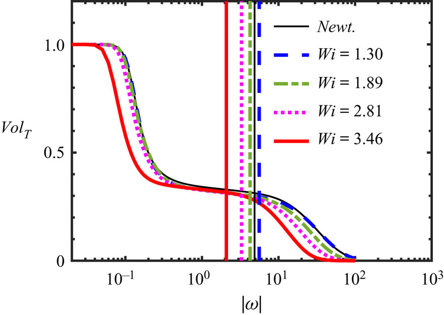
This is well illustrated in figure 1 which shows the volume fraction of the flow defined as turbulent ( $Vol_T (\omega _{th})$), whenever the local vorticity magnitude
 $(\omega _i \omega _i)^{1/2}$ is greater than
 $\omega _{th}$, for all the DNS used in the present work. It is clear that for a range of values of
 $\omega _{th}$,
 $1 \lesssim \omega _{th} \lesssim 10$ i.e. while varying
 $\omega _{th}$ by approximately one order of magnitude,
 $Vol_T (\omega _{th})$ changes very slowly, exhibiting a near plateau region. Similar profiles of
 $Vol_T (\omega _{th})$ have been observed in TNTI from many different flow types, e.g. da Silva, Taveira & Borrell (Reference da Silva, Taveira and Borrell2014b), which reflects the ‘sharpness’ of the TNTI, which was clearly apparent even from the early visualisations of this layer, e.g. Silva et al. (Reference Silva, Zecchetto and da Silva2018) observed that changing
 $\omega _{th}$ by more than 2 orders of magnitude resulted in this reference position moving about
 $\approx 1 \eta$.
Turbulent volume fraction ( $Vol_T$) as function of the vorticity magnitude threshold
 $|\omega |$, for all the DNS used in the present work, at the instants used in the subsequent SFT analysis. The vertical lines represent the detected thresholds for each case, obtained with the second derivative method i.e.
 ${\rm d}^2 Vol_T / {\rm d}|\omega |^2 (\omega _{th}) = 0$ (see main text for details).

The particular value of  $\omega _{th}$ used for each simulation is obtained from
 ${\rm d}^2 Vol_T / {\rm d} |\omega |^2 (\omega _{th}) = 0$ and is represented by a vertical line in figure 1, but it must be stressed that any other value taken from the same plateau of constant, or slowly evolving,
 $Vol_T (\omega _{th})$, results in virtually the same conditional statistics. The computation of
 $\omega _{th}$ using the above procedure can be difficult for some cases because the function
 $Vol_T (\omega _{th})$ may exhibit small scale oscillations for small values of
 $\omega _{th}$. In these cases one may need to apply a filter to the function
 $Vol_T (\omega _{th})$ before computing
 ${\rm d}^2 Vol_T / {\rm d} |\omega |^2$. No filtering was needed in the present cases.
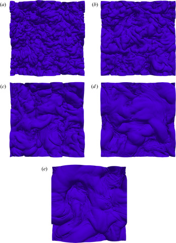
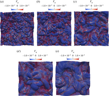
Figure 2 shows iso-surfaces of vorticity magnitude corresponding to the several simulations analysed in the present work. The IB corresponding to the Newtonian case (figure 2a) exhibits the typical features that have been observed in IB from many other flows (da Silva et al. Reference da Silva, Taveira and Borrell2014b). The IB is highly convoluted and exhibits a number of crests and troughs, spanning a range of large and small scales, which are imposed from the turbulent characteristics of the turbulent flow region. For the other (non-Newtonian) cases the size of the largest scales imprinted in the IB seems to increase as the Weissenberg number increases. This reflects the important modifications that the flow experiences due to the viscoelastic effects of the fluid, both from inside the turbulent core region of the flow, as well as from within the TNTI layer, as we will discuss below. In particular, the increasing size of the large scale convolutions of the IB reflects the increase of the turbulent integral scale of the flow as  $Wi$ increases, as observed in Valente et al. (Reference Valente, da Silva and Pinho2014). The values of
 $l_0$ in table 1 support this view. The increase of the integral scale of turbulence for a viscoelastic fluid, when compared with a Newtonian reference case, has been documented before in Liberzon et al. (Reference Liberzon, Holzner, Luthi, Guala and Kinzelbach2009) who compared turbulent fronts of water and of a viscoelastic fluid. In these experiments the integral scale was observed to have increased by approximately 30 % in the viscoelastic fluid (compared with water). This is precisely the increase of
 $l_0$ we observe here when comparing the Newtonian and the viscoelastic case with the highest Weissenberg number (see table 1).
Top view iso-surfaces of the IB, detected with the vorticity magnitude equal to the selected threshold ( $|\omega | = \omega _{th}$) for all the DNS used in the present work, at the instant used in the analysis: (a) Newtonian reference case; (b)
 $Wi = 1.30$; (c)
 $Wi = 1.89$; (d)
 $Wi = 2.81$; (e)
 $Wi = 3.46$.

3.2. Conditional statistics in relation to the TNTI layer
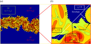
In the present work we compute statistics in relation to the distance from the ‘real’ IB surface, and not its envelope, which has been used in the great majority of the previous works dealing with the TNTI layer. Figure 3(a) shows contours of enstrophy in a side view of the entire flow domain in the  $(x,y)$ plane, for the Newtonian reference simulation. In the turbulent core region (TR) the enstrophy is above the enstrophy threshold detected, as explained in the previous section (
 $\omega > \omega _{th}$), whereas the irrotational region (IR) is represented by flow points below this threshold (
 $\omega < \omega _{th}$). The IB is represented by a solid dark line and corresponds to points with
 $\omega = \omega _{th}$.
Sketch of the procedure used to compute the conditional statistics in relation to the position of the IB for the Newtonian reference simulation. (a) Contours of enstrophy in a  $(x,y)$ plane showing the entire flow domain. The IB is represented by a solid dark line, which separates the TR and the IR flow regions; (b) magnification of a flow region near the TNTI layer showing the IB (solid dark line) and the IB interface (dashed white line). The figure shows also the local axis (normal to the local IB) that is used to collect the flow statistics in relation to the IB position. The origin of this axis coincides with the IB (
 $y_I = 0$) and the coordinates with
 $y_I>0$ and
 $y_I<0$ correspond to the turbulent and irrotational flow regions, respectively. The figure shows also that points from a nearby hole of non-turbulent flow within the turbulent region are not accounted for in the conditional statistics of the turbulent region.

Figure 3(b) shows the difference between the ‘true’ IB, which is used here to compute the conditional statistics, and the envelope of the IB. The local enstrophy gradient is used to define a three-dimensional (3-D) normal at each point of the IB, in the upper and lower shear layers, and any flow quantity of interest is collected into a grid defined on this 3-D axis at fixed distances  $y_I$, using a trilinear interpolation. The orientation of this 3-D normal is such that
 $y_I<0$ and
 $y_I>0$ correspond to the irrotational and turbulent regions, respectively (the IB is located at
 $y_I=0$). We denote the mean of a general quantity
 $\phi$ computed with this procedure as
 $\left \langle \phi \right \rangle _I$.
As in Westerweel et al. (Reference Westerweel, Fukushima, Pedersen and Hunt2009), points belonging to bubbles of irrotational flow within the turbulent region, and islands of turbulent flow inside the non-turbulent region, are automatically discarded from the statistical sample. In the present work, a single instantaneous field is used to compute the conditional statistics corresponding to each individual simulation, which is sufficient to obtain a good level of convergence of the desired quantities because of the large number of grid points available.
3.2.1. Conditional profiles of mean enstrophy and mean trace of the conformation tensor
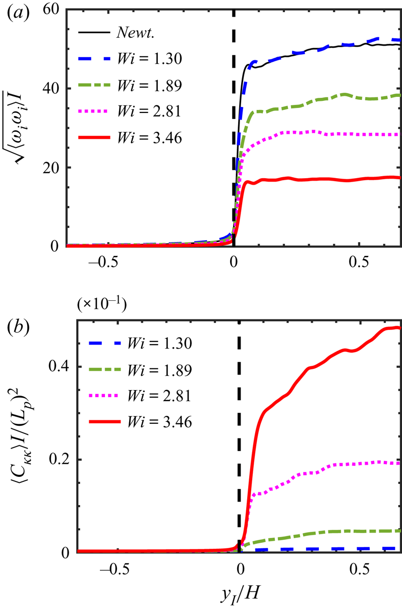
Figure 4(a,b) shows the conditional mean profiles of vorticity magnitude  $\left \langle ( \omega _i \omega _i )^{1/2} \right \rangle _I$ and (normalised) trace of the conformation tensor,
 $\left \langle C_{kk} \right \rangle _I / (L_{p})^2$, for each one of the simulations used in the present work. The distance to the IB is normalised with the size of the initial turbulent region
 $H$.
Conditional mean profiles of (a) vorticity magnitude  $\left \langle \sqrt { \omega _i \omega _i} \right \rangle _I$ and (b) (normalised) trace of the conformation tensor,
 $\left \langle C_{kk} \right \rangle _I / (L_{p})^2$, as a function of the distance from the IB position, for all the DNS used in the present work, at the instant used in the analysis.

In the Newtonian simulation the vorticity magnitude is virtually zero in the non-turbulent region and tends to a near constant value inside the turbulent core region, after experiencing a very sharp jump right after the IB position ( $0 \le y_I/H \le 0.05$). This jump occurs inside the TNTI layer, whereas the smaller vorticity increase observed afterward (
 $y_I/H > 0.05$) is associated with large scale inhomogeneities in the turbulent core region (Zecchetto & da Silva Reference Zecchetto and da Silva2021). Similar conditional enstrophy profiles have been reported in many different shear flows, including jets, mixing layers and boundary layers (e.g. Bisset, Hunt & Rogers Reference Bisset, Hunt and Rogers2002; Westerweel et al. Reference Westerweel, Fukushima, Pedersen and Hunt2005; Holzner et al. Reference Holzner, Liberzon, Nikitin, Kinzelbach and Tsinober2007; Watanabe, da Silva & Nagata Reference Watanabe, da Silva and Nagata2019).
Comparing these profiles for all the simulations used in the present work one observes that as  $Wi$ increases the enstrophy magnitude in the turbulent core region decreases. This result reflects one of the well-known effects of viscoelasticity in turbulent flows, namely that it depletes the turbulence at the small scales of motion (Valente et al. Reference Valente, da Silva and Pinho2014), a fact that is clearly apparent from the values of solvent viscous dissipation
 $\varepsilon ^{[s]}$ listed in table 1. For the Newtonian case the vorticity magnitude inside the turbulent core region
 $\omega ' = \sqrt {\left \langle \omega _i \omega _i \right \rangle _I}$ is well approximated by the relation
 $\omega ' \sim \tau _{\eta }^{-1}$, where
 $\tau _{\eta } = (\nu /\varepsilon )^{1/2}$ is the Kolmogorov time scale (Zecchetto & da Silva Reference Zecchetto and da Silva2021). Note that the same relation holds in the viscoelastic cases if we replace
 $\varepsilon$ and
 $\nu$ by
 $\varepsilon ^{[s]}$ and
 $\nu ^{[s]}$, respectively i.e.
 $\omega ' \sim (\varepsilon ^{[s]}/\nu ^{[s]})^{1/2}$. However, for high
 $Wi$ the theory of Lumley (Reference Lumley1973) can be employed to estimate
 $\omega '$. In short, at high
 $Wi$ the fluctuating polymer stresses and velocity gradients are strongly ‘coupled’ for length scales
 $r$ below a scale
 $r^{\ast }$, known as Lumley's scale, so that the time scale of the flow
 $\tau (l)$, associated with a given eddy size
 $l$, is imposed by the polymers relaxation time scale,
 $\tau (l) \sim \tau _p$. By using the inertial range scaling for the velocity scale
 $u(l) \sim (\varepsilon ^{[s]} l)^{1/3}$, and since
 $\tau (l) \sim l/u(l)$, one obtains Lumley's length and velocity scales,
 $r^{\ast } = \sqrt {\varepsilon ^{[s]} \tau _p^3}$ and
 $u^{\ast } = \sqrt {\varepsilon ^{[s]} \tau _p}$, respectively. Since for high
 $Wi$ the smallest time scale is
 $\tau _p$, the vorticity magnitude should scale as
 $\omega ' \sim \tau _p^{-1}$. This relation is reasonably well observed in the present data for the highest
 $Wi$, and explains why the vorticity magnitude in the turbulent core region of the flow decreases as
 $Wi$ (and
 $\tau _p$) increases. Apart from this, it is difficult to observe the effects of viscoelasticity in the details of the enstrophy jump across the TNTI layer, since the magnitude of the enstrophy jump at the interface and the thickness of this jump are not clearly dependent on the value of
 $Wi$.
The conditional mean profiles of trace of the conformation tensor,  $\left \langle C_{kk} \right \rangle _I / (L_{p})^2$ are also virtually zero (actually
 $3/(L_{p})^2$) in the non-turbulent region and display a constant or slowly evolving growth in the turbulent region. Since this quantity is proportional to the elastic energy stored in the polymer molecules the fact that
 $\left \langle C_{kk} \right \rangle _I / (L_{p})^2$ increases with
 $Wi$ is consistent with the behaviour of the enstrophy. Specifically, because part of the kinetic energy in the energy cascade is diverted into the polymer molecules, as
 $Wi$ increases, less energy is directly dissipated by the solvent and more is diverted to the polymers for storage/dissipation. The conditional mean profiles of the trace of the conformation tensor display also a sharp jump after the IB for all the simulations used in the present work, but have an associated thickness that seems to be slightly larger than the thickness of the corresponding enstrophy jump. This may imply that, compared with the enstrophy, the viscoelastic mechanisms need more time to adjust to the dramatic inhomogeneity characteristic of TNTIs.
In the next section we address the detailed enstrophy budgets across the TNTI in order to understand this interplay between the solvent and polymer dynamics within TNTI layers from viscoelastic fluids.
4. Enstrophy budgets in TNTIs of viscoelastic fluids
By applying the curl operator to (2.2) and after multiplying by the vorticity vector  $\omega _i = \epsilon _{ijk} \partial u_k / \partial x_j$ we obtain the equation governing the enstrophy
 $\varOmega = \omega _i \omega _i/2$ for a viscoelastic fluid
 \begin{equation} \underbrace{{\dfrac{{\rm D}}{{\rm D}t} \left( \dfrac{\omega_i \omega_i}{2} \right)}}_{T_{\varOmega}} = \underbrace{\omega_i \omega_j S_{ij} }_{P_\varOmega} + \underbrace{\nu^{[s]} \dfrac{\partial^2}{\partial x_j \partial x_j} \left( \dfrac{\omega_i \omega_i}{2} \right)}_{D_\varOmega} - \underbrace{\nu^{[s]} \left( \dfrac{\partial \omega_i}{\partial x_j} \dfrac{\partial \omega_i}{\partial x_j} \right) }_{\varepsilon_\varOmega} + \underbrace{\omega_i \epsilon_{nji} \dfrac{\partial^2 \sigma_{mj}^{[p]}}{\partial x_m \partial x_n} }_{V_\varOmega},\end{equation}
where the first three terms on the right-hand side of (4.1) represent the total variation of enstrophy ( $T_{\varOmega }$), caused by enstrophy production (
 $P_{\varOmega }$), viscous diffusion (
 $D_{\varOmega }$) and viscous dissipation (
 $\varepsilon _{\varOmega }$), respectively. The last term represents the viscoelastic production resulting from the interactions between the vorticity field and the viscoelastic stresses, and is absent in classical (Newtonian) turbulence.
Figure 5 shows the conditional enstrophy budgets, obtained by averaging all the terms in (4.1) in relation to the distance from the IB, for all the simulations used in the present work. As in figure 4 the IB is located at  $y_I/H=0$ and the non-turbulent and turbulent regions are at
 $y_I<0$ and
 $y_I>0$, respectively.
Conditional enstrophy budgets for all the simulations used in the present work, obtained by averaging all the terms in (4.1) in relation to the distance from the IB as described in § 3.2.1: thin/solid/dark line – total variation ( $T_{\varOmega }$); long dashed/blue line – enstrophy production (
 $P_{\varOmega }$); dashed/green line – viscous diffusion (
 $D_{\varOmega }$); dotted/magenta line – viscous dissipation (
 $\varepsilon _{\varOmega }$); solid/red line – viscoelastic production (
 $V_{\varOmega }$). The IB is located at
 $y_I/H=0$ and the non-turbulent and turbulent regions are at
 $y_I<0$ and
 $y_I>0$, respectively. The distance from the IB (
 $y_I$) is normalised by the size of the initial turbulent region
 $H$: (a) Newtonian (reference) case; (b)
 $Wi = 1.30$; (c)
 $Wi = 1.89$; (d)
 $Wi = 2.81$; (e)
 $Wi = 3.46$.

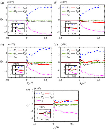
The enstrophy budgets for the Newtonian case (figure 5a) are similar to the ones observed in numerous other works (da Silva et al. Reference da Silva, Hunt, Eames and Westerweel2014a): all the enstrophy governing terms are virtually zero in the non-turbulent region  $y_I/H < 0$, while deep inside the turbulent core region (
 $y_I/H \gtrsim 0.3$) the enstrophy production and viscous dissipation roughly balance
 $\left \langle P_{\varOmega } \right \rangle _I \approx \left \langle \varepsilon _{\varOmega } \right \rangle _I$, and the viscous diffusion is negligible
 $\left \langle D_{\varOmega } \right \rangle _I \approx 0$. It is noteworthy that, in the turbulent core region and for the Newtonian and low
 $Wi$ cases, the enstrophy production normalised by the Kolmogorov time scale is
 $P_{\varOmega } \tau _{\eta }^3 = P_{\varOmega } / (u_{\eta }/\eta )^3 \approx 0.2$, which is the same observed for a Newtonian fluid (Zecchetto & da Silva Reference Zecchetto and da Silva2021), where in the viscoelastic cases the Kolmogorov time scale is computed as described before,
 $\tau _{\eta } = (\nu ^{[s]} / \varepsilon ^{[s]})^{1/2}$. This relation falls to
 $P_{\varOmega } \tau _{\eta }^3 \approx 0.12$ for the highest
 $Wi$ case, likely due to the decrease in the alignment between the vorticity and strain induced by the viscoelasticity (Cocconi et al. Reference Cocconi, De Angelis, Frohnapfel, Baevsky and Liberzon2017). When moving from the non-turbulent into the turbulent region the enstrophy increases initially (
 $y_I/H \approx 0.01$) by viscous diffusion, which is the most important term at that location
 $\left \langle D_{\varOmega } \right \rangle _I \gg \left \langle P_{\varOmega } \right \rangle _I$, while later on (
 $0.01 \lesssim y_I/H \lesssim 0.03$) enstrophy production takes over,
 $\left \langle P_{\varOmega } \right \rangle _I \gg \left \langle D_{\varOmega } \right \rangle _I$. The slower increase observed in the enstrophy production
 $\left \langle P_{\varOmega } \right \rangle _I$ between
 $0.1 \lesssim y_I/H \lesssim 0.3$ is caused by the adjustment of the flow to large scale inhomogeneities (Zecchetto & da Silva Reference Zecchetto and da Silva2021).
In the viscoelastic cases (figure 5b–e) a new term exists – viscoelastic production ( $V_{\varOmega }$) – which adds new complexity to the mechanism of enstrophy increase across the TNTI layer. The first observation regarding this term is that its source/sink nature (mean positive/negative) inside the turbulent core region depends on the Weissenberg number. Whereas the viscoelastic production is negative, and thus tends to decrease the mean value of enstrophy in the turbulent core region, for
 $Wi = 1.30$ and
 $Wi = 1.89$, it becomes positive (increasing the mean value of enstrophy) for
 $Wi = 2.81$ and
 $Wi = 3.46$. Moreover, the mean value of
 $\left \langle V_{\varOmega } \right \rangle _I$ well inside the turbulent core, seems to be a monotonic increasing function of
 $Wi$ for all the cases considered. We recover
 $\left \langle V_{\varOmega } \right \rangle _I = -3998.0, -1380.0, 457.3$ and
 $598.5$ at
 $y_I/H = 0.67$ for the cases with
 $Wi = 1.30, 1.89, 2.81$ and
 $3.46$ respectively. Furthermore, for the simulation with the highest value of
 $Wi$ the viscoelastic production is as important as the production by vortex stretching,
 $\left \langle V_{\varOmega } \right \rangle _I \approx \left \langle P_{\varOmega } \right \rangle _I$.
This changing nature of  $V_{\varOmega }$, i.e. its dependence on
 $Wi$, is certainly linked with the modified energy cascade mechanism that exists in viscoelastic turbulence (compared with Newtonian turbulence) and which changes with the Weissenberg number. As described in e.g. Valente et al. (Reference Valente, da Silva and Pinho2014, Reference Valente, da Silva and Pinho2016) for low values of
 $Wi$ the kinetic energy spectrum exhibits a classical Kolmogorov–Obukhov inertial range
 $E(k) \sim k^{-5/3}$, which is recovered also at very high values of
 $Wi$, while for intermediate values of
 $Wi$ the kinetic energy spectrum displays an inertial–elastic region with
 $E(k) \sim k^{-3}$. The rational for this behaviour is the following. While at low
 $Wi$ the energy cascade mechanism remains similar to Newtonian turbulence, although with an additional dissipation mechanism caused by the polymer molecules, at very high values of
 $Wi$ the solvent and polymer dynamics are totally de-correlated, because the energy input created by the large scales of motion is transferred into the polymers at large scales. However, for intermediate values of
 $Wi$, a fraction of the energy injected by the large scales of motion into the solvent is transferred and stored in the polymers, thereby decreasing the ‘activity’ in the intermediate and small scales of motion in the solvent.
In agreement with the energy cascade picture described above, figure 5(b,c) corresponding to low  $Wi$, shows that adding the polymer molecules results in a new (additional) dissipation mechanism, as shown by the negative value of the viscoelastic production (
 $V_{\varOmega }$). In contrast, for very high values of
 $Wi$, figure 5d,e), the enstrophy production becomes positive, which is consistent with the mechanism described in Valente et al. (Reference Valente, da Silva and Pinho2014), where the energy cascade is altered by the existence of a new mechanism in which the polymers gain energy from the flow at small scales but cannot dissipate this extra energy and inject it back into the solvent dissipative scales. It is interesting to observe, however, that for all cases, even for low
 $Wi$ where we have
 $\left \langle V_{\varOmega } \right \rangle _I < 0$, in the turbulent core region, the viscoelastic production is always positive at the IB i.e.
 $\left \langle V_{\varOmega } \right \rangle _I \ge 0$ at
 $y_I/H \approx 0$. This result is interesting because it suggests that the mechanisms influencing the viscoelastic production may work differently inside the TNTI layer and in the turbulent core region.
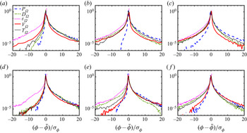
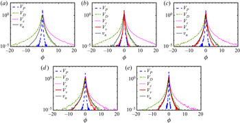
In order to analyse this in more detail figure 6 shows the probability density functions (p.d.f.s) of the several terms governing the enstrophy (4.1) for the two limiting viscoelastic simulations –  $Wi=1.30$ and
 $Wi = 3.46$ – at several locations within the TNTI: at the VSL, at the TSL, and inside the turbulent core region.
The p.d.f.s of the several terms governing the enstrophy transport equation (4.1) for the viscoelastic simulations with  $Wi=1.30$ (a–c) and
 $Wi = 3.46$ (d–f), at several locations within the TNTI layer: (a,d) at the VSL (in the point of maximum enstrophy viscous diffusion); (b,e) at the TSL (in middle of the region of growing enstrophy production); and at the turbulent core region (c,f).

As expected the general shape of the p.d.f.s of enstrophy production and viscous dissipation ( $P_{\varOmega }$ and
 $\varepsilon _{\varOmega }$) do not change while crossing the TNTI layer i.e. when moving from the IB into the turbulent core region: the p.d.f. of the dissipation is always negatively skewed (indeed all instantaneous values of
 $\varepsilon _{\varOmega }$ are negative), whereas the p.d.f.s of
 $P_{\varOmega }$ is positively skewed, with a predominance of production by vortex stretching over dissipation by vortex compression. Also, the p.d.f. of enstrophy diffusion changes from being positively skewed in the VSL into being negatively skewed in the TSL and in the turbulent core regions, which implies a viscous transport of enstrophy from the turbulent core region into the non-turbulent region. The behaviour of the viscous diffusion in the present viscoelastic TNTIs is then similar to virtually all reported TNTIs of Newtonian fluids (da Silva et al. Reference da Silva, Hunt, Eames and Westerweel2014a). Thus, the viscoelasticity does not affect, at least in a direct way, the behaviour of the other enstrophy governing equation terms, apart from decreasing the magnitude of each one of these terms as
 $Wi$ increases.
Recall that the p.d.f.s of the terms governing (4.1) have been analysed in isotropic turbulence by Cai, Li & Zhang (Reference Cai, Li and Zhang2010), and that the shape of the present p.d.f.s (in the turbulent core region – figure 6c–f), as well as their dependence on  $Wi$ closely resemble the ones from Cai et al. (Reference Cai, Li and Zhang2010), including the fact that increasing
 $Wi$ results on a depletion of the activity in the small scales of motion, and a concomitant decrease in the frequency of the extreme events in these terms.
In contrast the shape of the p.d.f. of the viscoelastic production term ( $V_{\varOmega }$) changes both with the position within the TNTI layer and with
 $Wi$. As expected from the conditional mean values of
 $V_{\varOmega }$ analysed above, for the lower
 $Wi$ values e.g.
 $Wi = 1.30$ (figure 6b,c) and
 $Wi = 1.89$ (not shown) the viscoelastic production is negative both in the TSL and in the turbulent core region of the flow, causing therefore a decrease of enstrophy in the flow at these locations. In contrast, for the higher
 $Wi$
 $V_{\varOmega }$ is always positively skewed.
However, for all (low and high) values of  $Wi$ the p.d.f. of
 $V_{\varOmega }$ is always positively skewed at the IB (
 $y_I/H=0$ – not shown) and also inside the VSL (figure 6a,d) i.e. even though
 $V_{\varOmega }$ can represent either a source or a sink of the total enstrophy in the turbulent core region of the flow, depending on
 $Wi$, the positive (source) contributions always dominate close to the IB, showing that the mechanisms of the viscoelastic production are somehow affected by the peculiar dynamics of the flow near the IB.
Again, while the changing nature of the viscoelastic production inside the turbulent core region of the flow, i.e. its  $Wi$ dependence, can surely be attributed to the changing energy cascade mechanism described above when discussing the mean value of this quantity
 $\left \langle V_{\varOmega } \right \rangle _I$, this cannot explain what happens near the IB or in the VSL, since no true kinetic energy cascade exists at these locations (Watanabe et al. Reference Watanabe, da Silva and Nagata2019). The particular dynamics of the flow near the IB must be somehow responsible for this particular feature of the viscoelastic production.
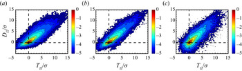
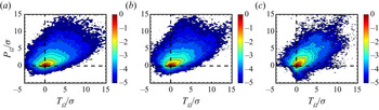
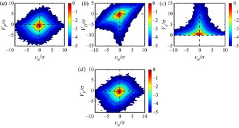
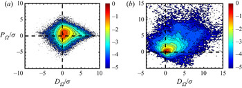
In order to assess this further the following figures show joint probability density functions (j.p.d.f.) of several of the terms governing the enstrophy at several locations inside the TNTI layer. The j.p.d.f.s between the total variation ( $T_{\varOmega }$) and viscous diffusion (
 $D_{\varOmega }$) (figure 7), and between total variation (
 $T_{\varOmega }$) and production (
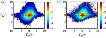
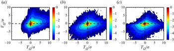
 $P_{\varOmega }$) (figure 8) essentially show that the same results already described in Taveira et al. (Reference Taveira, Diogo, Lopes and da Silva2013) for a Newtonian fluid, are also valid for the present viscoelastic flow. Specifically, that moving from the non-turbulent into the turbulent region, the enstrophy increases initially (in the VSL) by the action of viscous diffusion and latter (in the TSL) by vortex stretching. The new results obtained for the viscoelastic cases show only a mild effect of
 $Wi$ on these facts, and suggest that as
 $Wi$ increases the enstrophy viscous diffusion (inside the VSL) and the enstrophy production (inside the TSL), contribute slightly less to the growth of the total enstrophy, as
 $Wi$ increases.
The j.p.d.f.s of enstrophy variation ( $T_{\varOmega }$) and enstrophy viscous diffusion (
 $D_{\varOmega }$) at the VSL for the simulations with (a)
 $Wi=0$ (Newtonian), (b)
 $Wi=1.30$ and (c)
 $Wi = 3.46$. The variables are centred and normalised by their r.m.s. values. In these and all the other j.p.d.f.s of this paper the lower limit of the iso-lines displayed corresponds to the level
 $10^{-5}$, and the j.p.d.f.s are normalised so that
 $\iint p (x,y)\,{{\rm d}\kern0.06em x}\,{{\rm d}y} =1$.

The j.p.d.f.s of enstrophy variation ( $T_{\varOmega }$) and enstrophy production (
 $P_{\varOmega }$) at the turbulent superlayer (TSL) for the simulations with (a)
 $Wi=0$ (Newtonian), (b)
 $Wi=1.30$ and (c)
 $Wi = 3.46$. The variables are centred and normalised by their r.m.s. values.

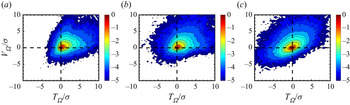
Figure 9 shows the j.p.d.f. between the total variation ( $T_{\varOmega }$) and the viscoelastic production (
 $V_{\varOmega }$). The slight positive correlation between the two quantities attests that this mechanism indeed contributes to the growth of enstrophy right at the IB position (
 $y_I/H=0$), and the next sets of three figures show the evolution of these j.p.d.f.s across the TNTI layer for
 $Wi=1.30$ (figure 10) and
 $Wi = 3.46$ (figure 11). The j.p.d.f.s at the VSL confirm the result observed at the IB for both simulations
 $Wi=1.30$ and
 $3.46$, showing a more well-defined positive correlation between
 $T_{\varOmega }$ and
 $V_{\varOmega }$. However, it is clear that the shapes of the j.p.d.f.s at the TSL for
 $Wi=1.30$ (figure 10b) and
 $Wi=3.46$ (figure 11b) are qualitatively different. Whereas for
 $Wi=1.30$ the correlation between
 $T_{\varOmega }$ and
 $V_{\varOmega }$ comes from negative values of both quantities i.e. the enstrophy decreases due to negative values of
 $V_{\varOmega }$ (see figure 10b), for
 $Wi=3.46$ it clearly comes from positive values of both quantities (see figure 11b). The same is true in the turbulent core region, although the correlation between
 $T_{\varOmega }$ and
 $V_{\varOmega }$ seems to be always stronger for
 $Wi=3.46$ than for
 $Wi=1.30$.
The j.p.d.f.s of enstrophy variation ( $T_{\varOmega }$) and viscoelastic production (
 $V_{\varOmega }$) at the IB for the simulations with (a)
 $Wi=1.30$ and (b)
 $Wi = 3.46$. The variables are centred and normalised by their r.m.s. values.

The j.p.d.f.s of enstrophy variation ( $T_{\varOmega }$) and viscoelastic production (
 $V_{\varOmega }$) for the simulation with
 $Wi=1.30$, at the VSL (a); TSL (b) and turbulent core region (c). The variables are centred and normalised by their r.m.s. values.

The j.p.d.f.s of enstrophy variation ( $T_{\varOmega }$) and viscoelastic production (
 $V_{\varOmega }$) for the simulation with
 $Wi=3.46$, at the VSL (a); TSL (b) and turbulent core region (c). The variables are centred and normalised by their r.m.s. values.

To summarise, the analysis of the terms governing the enstrophy equation (4.1) across the TNTI layer show that in viscoelastic fluids a new term exists – the viscoelastic production – that contributes significantly to the dynamics of the enstrophy in the layer (as in the turbulent core region). While this term can be positive or negative in the turbulent core region, depending on  $Wi$, it is consistently positive near the IB and within the VSL. Thus, the mechanism of enstrophy generation across the TNTI layer is different to the one observed in Newtonian fluids, and this may have an impact on the structure of the TNTI layer itself. This issue is addressed in the next section.
5. The structure of the TNTI layer for viscoelastic flows
As described in the introduction the structure of the TNTI layer in Newtonian fluids has been extensively analysed. Its definition is based on the relative importance of the two mechanisms driving the growth of the enstrophy from the non-turbulent region into the turbulent core region of the flow. The TNTI layer is comprised of two sublayers: the viscous superlayer (VSL) where the viscous diffusion dominates, and the turbulent sublayer (TSL) where the production by vortex stretching becomes dominant (see Silva et al. (Reference Silva, Zecchetto and da Silva2018) and references therein).
Since the TNTI layer in viscoelastic flows has an additional new physical mechanism due to the interaction between the vorticity and polymer stresses (viscoelastic production,  $V_{\varOmega }$), it is important to analyse whether the classical (Newtonian) structure of the TNTI layer holds also in viscoelastic flows, or if, on the contrary, the new mechanism leads to the emergence of a sublayer within the TNTI layer.
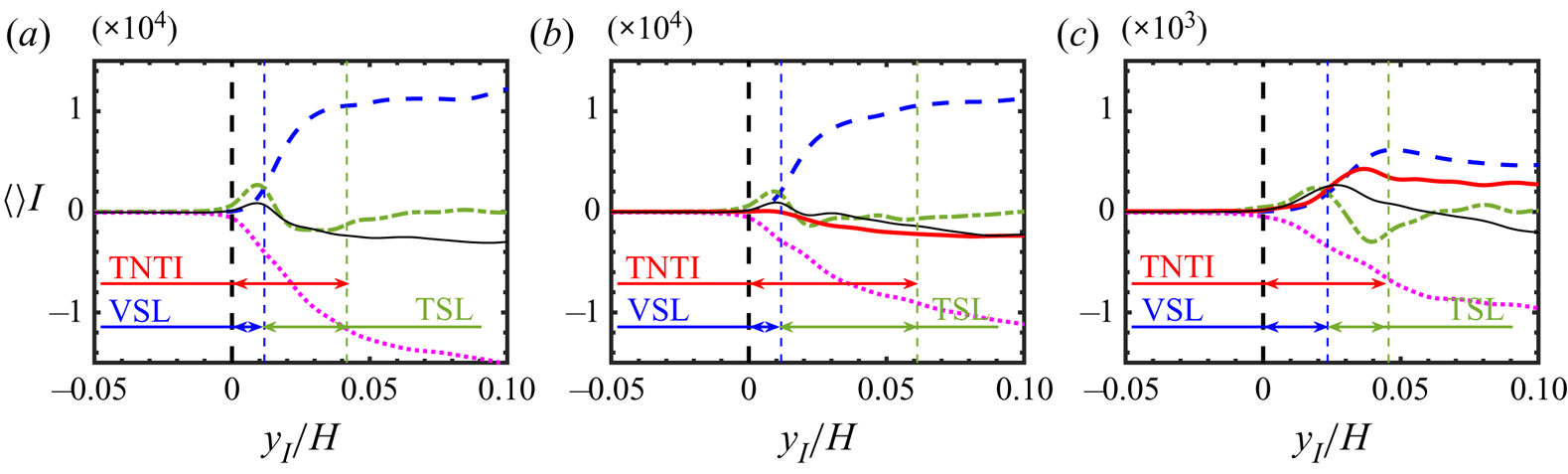
To clarify this, figure 12 shows the conditional enstrophy budgets for the Newtonian (reference) simulation, and for the simulations with  $Wi=1.30$ and
 $Wi=3.46$, indicating the extents of the VSL and TSL, which added together define the total extent of the TNTI layer. The Newtonian case (figure 12a) allows one also to recall the exact definitions used for the two sublayers: the VSL is defined as the distance from the IB to the point where the enstrophy viscous diffusion crosses the enstrophy production,
 $D_{\varOmega } = P_{\varOmega }$, while the TSL is defined as the distance between this point and the location of the first maximum of enstrophy (which is not shown in figure 12). As in Silva et al. (Reference Silva, Zecchetto and da Silva2018) we define the boundary between the VSL and TSL by the point where the enstrophy viscous diffusion intersects the enstrophy production,
 $D_{\varOmega } = P_{\varOmega }$.
Conditional mean profiles of the terms in (4.1) showing the extent of the VSL, TSL and the total extent of the TNTI layer, for the simulations with: (a) Newtonian fluid; (b)  $Wi=1.30$; (c)
 $Wi=3.46$. The colours and line types for each term are the same as in figure 5 e.g. the viscoelastic production (
 $V_{\varOmega }$) is represented in solid/red line.

Looking into the enstrophy budgets for the case  $Wi=1.30$ it is clear that the conditional mean viscoelastic production,
 $V_{\varOmega }$, never overtakes any of the other enstrophy equation terms, since the mean profile of this term is always slightly negative (except at the IB). For
 $Wi=3.46$ the viscoelastic production closely follows the production by vortex stretching,
 $P_{\varOmega } \approx V_{\varOmega }$, until
 $y_I/H \approx 0.04$ without ever becoming more important. Therefore we conclude that, at least for the range of values of
 $Wi$ considered in this study, a viscoelastic sublayer i.e. a sublayer where this term might be dominant, cannot be observed, so that the structure of the TNTI layer remains the same as for Newtonian fluids. However, the relative size of each one of these sublayers is affected by the Weissenberg number as the results listed in table 2 clearly show.
Mean thickness of the VSL  $\left \langle \delta _{VSL} \right \rangle$, TSL
 $\left \langle \delta _{TSL} \right \rangle$ and the total extent of the TNTI layer
 $\left \langle \delta _{TNTI} \right \rangle$, for the simulations with Newtonian and viscoelastic fluids analysed in the present work. The several mean thicknesses are normalised by the size of the initial turbulent region (
 $H$) and by the Kolmogorov micro-scale (
 $\eta$).

This table lists the values of the mean thicknesses of the TNTI layer, and of its two sublayers, for all the simulations used in the present work. The mean thicknesses are normalised by the size of the initial turbulent region  $H$, and by the Kolmogorov micro-scale
 $\eta$, computed at the turbulent core region of the flow. It is instructive to start this analysis by looking into the values of the mean thicknesses using the normalisation with
 $H$. It is clear that
 $\left \langle \delta _{TNTI} \right \rangle / H$ is not a monotonic function of
 $Wi$, as its value starts to increase with
 $Wi$, reaching
 $\left \langle \delta _{TNTI} \right \rangle / H \approx 0.07$ until
 $Wi=1.89$, but subsequently decreases to
 $\left \langle \delta _{TNTI} \right \rangle / H \approx 0.040$ for
 $Wi=2.81$ and
 $3.46$. This is explained mainly by a similar non-monotonic behaviour of the mean thickness of the TSL,
 $\left \langle \delta _{TSL} \right \rangle / H$, since the mean thickness of the VSL, which, as expected is always much smaller than the TSL, is approximately constant with
 $\left \langle \delta _{VSL} \right \rangle / H \approx 0.01-0.02$ for all cases.
Recently, it has been demonstrated that, for a Newtonian fluid, provided the Reynolds number is sufficiently high, the mean (and local) thicknesses of the TNTI layer and its two sublayers, all scale with the Kolmogorov micro-scale (Silva et al. Reference Silva, Zecchetto and da Silva2018). The explanation has to do with the fact that the sharp vorticity jump observed across the TNTI layer is caused by the first row of structures of intense vorticity, with mean diameters close to  $D_{ivs} \approx 10 \eta$, which themselves define the contours and shape of the IB surface and the size of the thickness of the TNTI layer.
The results in table 2 show that for the smaller values of the Weissenberg number  $Wi=1.30$ and
 $1.89$, the mean values of the TNTI thickness are in the range
 $\left \langle \delta _{TNTI} \right \rangle / \eta \approx 10-14$ which is very close to the values observed for Newtonian fluids (Silva et al. Reference Silva, Zecchetto and da Silva2018). This is consistent with the idea that at low or moderate values of the Weissenberg number turbulent viscoelastic flows display small scale eddy structures that are similar to the ones observed in Newtonian turbulence. The slightly smaller value obtained here for the Newtonian case is consistent with the relatively low Reynolds number corresponding to this simulation.
However, for  $Wi=2.81$ and
 $3.46$ we obtain
 $\left \langle \delta _{TNTI} \right \rangle / \eta \approx 6$ which shows that the scaling of the TNTI layer for these high Weissenberg number cases is clearly different to the one obtained for Newtonian fluids. This comes as no surprise as it is well known, e.g. Ferreira et al. (Reference Ferreira, Pinho and da Silva2017), that for high Weissenberg numbers the regions of intense vorticity are organised into sheets, which have a smaller thickness than the typical diameter of the intense vorticity structures. Since the IB is defined by a low vorticity threshold created at the edge of these structures it is normal to expect a smaller thickness of the TNTI layer, when this thickness is normalised by the Kolmogorov micro-scale. Note, however, that for the higher Weissenberg number cases the Kolmogorov micro-scale is actually much higher than in similar Newtonian or low Weissenberg number flows, so the question here is more of deciding what is the smallest characteristic scale of motion in viscoelastic turbulent flows (at high Weissenberg number), a topic that is probably outside the scope of the present paper. The slightly smaller value of the mean thickness of the TSL observed in the Newtonian case,
 $\left \langle \delta _{TNTI} \right \rangle / \eta \approx 7$ compared with
 $\left \langle \delta _{TNTI} \right \rangle / \eta \approx 11$ for
 $Wi=1.30$ and
 $Wi=1.89$, can probably be attributed to the method employed for this estimation not being very accurate - it measures the end of the TSL (and TNTI) by the location of the first maximum in the conditional mean enstrophy profiles (compare figure 12a,b). The more accurate methods described in Silva et al. (Reference Silva, Zecchetto and da Silva2018) and Zecchetto & da Silva (Reference Zecchetto and da Silva2021) cannot be used in the present viscoelastic cases until the size of the smallest scales of motion in these flows is finally settled. A final remark concerns the mean thickness of the VSL. Table 2 shows that in all cases the mean thickness of the VSL is almost the same, with
 $\left \langle \delta _{VSL} \right \rangle / \eta \approx 2-3$, which is close to the values typically observed in Newtonian turbulence.
To summarise, the present results show that, for the range of Weissenberg numbers investigated, the structure of the TNTI layer is similar to the one found in Newtonian interfaces, and is comprised of a VSL, dominated by the enstrophy solvent viscous diffusion, followed by a TSL, dominated by the enstrophy production (for low and moderate  $Wi$), or simultaneously by the enstrophy production and viscoelastic production (for high
 $Wi$). Moreover, the scaling of the TNTI layer, for low and moderate values of
 $Wi$ is similar to the scaling of the TNTI layer for Newtonian fluids, however, for high
 $Wi$ a different scaling exists, probably associated with the size of the sheet structures that dominate the flow for high
 $Wi$.
In the next section we investigate how the several features of the TNTI layer described above explain the smaller spreading rates observed in viscoelastic fluids compared with Newtonian fluids.
6. TE for viscoelastic flows
One notable feature of viscoelastic turbulent free flows is the spectacular decrease of the entrainment rates compared with Newtonian flows. In turbulent viscoelastic planar jets this decreased entrainment rate is manifested by much smaller spreading rates, compared with the typical (Newtonian) reference values (Guimarães et al. Reference Guimarães, Pimentel, Pinho and da Silva2020). Liberzon et al. (Reference Liberzon, Holzner, Luthi, Guala and Kinzelbach2009) and Cocconi et al. (Reference Cocconi, De Angelis, Frohnapfel, Baevsky and Liberzon2017) observed a similar trend in free-shear turbulence, where the mean propagating speed of the turbulent front is smaller for a solution of water carrying polymer molecules, than for water alone.
This issue is analysed here by looking into the entrainment velocity  $v_n$, which is the velocity of the turbulent front relative to the fluid, and the entrainment rate
 $Q_l$, which can be estimated by
 $Q_l \sim v_n A_{IB}$, where
 $A_{IB}$ is the area of the IB.
The local entrainment velocity  $v_n$ can be computed by considering that the velocity of an iso-surface of constant enstrophy, e.g. the iso-surface of low enstrophy corresponding to the IB,
 $u^{B}_i$, can be computed as the sum of the local fluid velocity
 $u_i$, and the velocity of the IB relative to the fluid,
 $u^{R}_i$ (
 $u^{B}_i = u_i + u^{R}_i$), where the local entrainment velocity, i.e. the velocity of the IB relative to the fluid is
 $u^{R}_i = v_n n_i$, where
 \begin{equation} \boldsymbol{n} = \dfrac{\boldsymbol{\nabla} \left( \dfrac{\omega_i \omega_i}{2} \right)}{\left\vert \boldsymbol{\nabla} \left( \dfrac{\omega_i \omega_i}{2} \right)\right\vert} \end{equation}
is the local surface normal at the IB (Wolf et al. Reference Wolf, Luthi, Holzner, Krug and Kinzelbach2012). Since the iso-surface of enstrophy corresponding to the IB, where the enstrophy is  $\omega ^{th}_i \omega ^{th}_i / 2$, moves with constant enstrophy, we can write
 \begin{equation} \frac{{\rm D} \left( \omega^{th}_i \omega^{th}_i / 2 \right)}{{\rm D} t} = \frac{\partial \left( \omega^{th}_i \omega^{th}_i / 2 \right)}{\partial t} + (u_j + u^{R}_j) \frac{\partial \left( \omega^{th}_i \omega^{th}_i / 2 \right)}{\partial x_j} = 0, \end{equation}
where the entrainment velocity can be computed as
 \begin{equation} v_n ={-} \frac{1}{\left\vert \boldsymbol{\nabla} \left( \dfrac{\omega_i \omega_i}{2} \right) \right\vert} \dfrac{{\rm D} \left( \dfrac{\omega_i \omega_i}{2} \right)}{{\rm D} t}, \end{equation}
which leads to the final equation for the computation of the entrainment velocity after substitution by (4.1) for the enstrophy variation, (Wolf et al. Reference Wolf, Luthi, Holzner, Krug and Kinzelbach2012; Watanabe et al. Reference Watanabe, Sakai, Nagata, Ito and Hayase2015)
 \begin{equation} v_n ={-} \underbrace{\dfrac{\omega_i \omega_j S_{ij}}{\left|\boldsymbol{\nabla} \left( \dfrac{\omega_i \omega_i}{2} \right) \right|} }_{V_P} - \underbrace{\dfrac{\nu^{[s]} \dfrac{\partial^2}{\partial x_j \partial x_j} \left( \dfrac{\omega_i \omega_i}{2} \right)}{\left|\boldsymbol{\nabla} \left( \dfrac{\omega_i \omega_i}{2} \right) \right|}}_{V_D} + \underbrace{\dfrac{\nu^{[s]} \left( \dfrac{\partial \omega_i}{\partial x_j} \dfrac{\partial \omega_i}{\partial x_j} \right)}{\left|\boldsymbol{\nabla} \left( \dfrac{\omega_i \omega_i}{2} \right) \right|} }_{V_{\varepsilon}} - \underbrace{\dfrac{\omega_i \epsilon_{nji} \dfrac{\partial^2 \sigma_{mj}^{[p]}}{\partial x_m \partial x_n}}{\left|\boldsymbol{\nabla} \left( \dfrac{\omega_i \omega_i}{2} \right) \right|} }_{V_V}, \end{equation}
and where all the terms in the equation are to be evaluated at the IB i.e. at  $y_I=0$. The first three terms on the right-hand side of (6.4) represent the contributions from the enstrophy production (
 $V_P$), viscous diffusion (
 $V_D$) and viscous dissipation (
 $V_{\varepsilon }$) and exist also for Newtonian fluids, while the last contribution, due to the viscoelastic production (
 $V_V$), exists only for viscoelastic fluids. The derivation of (6.4) was first done by Holzner & Luthi (Reference Holzner and Luthi2011) for a Newtonian fluid, while the form shown above represents a natural extension for viscoelastic fluids.
Note that  $v_n$ adopts positive values when the entrainment velocity is oriented in the direction of the enstrophy gradient, which means that the local
 $v_n$ on a section of the surface spreading into the irrotational flow region is negative, while locally positive values of
 $v_n$ imply that the fluid at the IB is moving in the direction of the turbulent region.
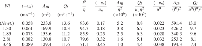
Table 3 shows the values of the mean entrainment velocity  $v_n$, surface area of the IB
 $A_{IB}$ and estimated flow rate
 $Q_l$ for all the simulations used in the present work. The mean entrainment velocity is always negative, both for the Newtonian case, which agrees with Wolf et al. (Reference Wolf, Luthi, Holzner, Krug and Kinzelbach2012) and Watanabe et al. (Reference Watanabe, Sakai, Nagata, Ito and Hayase2015), and for the viscoelastic case, which agrees with Cocconi et al. (Reference Cocconi, De Angelis, Frohnapfel, Baevsky and Liberzon2017). The mean entrainment velocity varies significantly with the Weissenberg number, increasing with
 $Wi$ and exhibiting higher values for the simulation with the higher Weissenberg number,
 $Wi = 3.46$, with
 $\left \langle -v_n \right \rangle = 0.089$, in contrast to
 $\left \langle -v_n \right \rangle = 0.061$ for
 $Wi=1.30$. Liberzon et al. (Reference Liberzon, Holzner, Luthi, Guala and Kinzelbach2009) mentions that in his experiments the entrainment velocity is larger for a viscoelastic fluid than for water, which is consistent with what is observed in the present DNS. Notice, however, that the present simulations are different from the experiments of Liberzon et al. (Reference Liberzon, Holzner, Luthi, Guala and Kinzelbach2009) and the experiments and simulations of Cocconi et al. (Reference Cocconi, De Angelis, Frohnapfel, Baevsky and Liberzon2017) in one aspect. Whereas in Liberzon et al. (Reference Liberzon, Holzner, Luthi, Guala and Kinzelbach2009) a constant energy input drives the turbulent front both in the case of water and of water carrying polymers, in the present DNS the turbulence inside the turbulent core region is actually (slowly) decaying in time, and for this reason different levels of energy are driving the different simulated interfaces. The power input
 $P$ in all cases can be estimated by using the data (in table 1) from the large scales of motion,
 $P \sim K^{3/2}/l \sim (u^0)^3/l^0$, and consistently decreases as
 $Wi$ increases. Additionally, the integral scale of turbulence increases with
 $Wi$ and it is natural to expect that bigger sized large scale eddies will result in bigger tangential velocities in their periphery, and therefore also in bigger entrainment velocities.
Mean entrainment velocity  $\left \langle v_{n} \right \rangle$, surface area of the IB
 $A_{IB}$ and flow rate
 $Q_l$, for all the simulations carried out in the present work. These quantities are also shown when normalised by the Kolmogorov velocity
 $u_{\eta }$ and length scale
 $\eta$, computed inside the turbulent core region, and also with the initial (HIT) r.m.s. velocity
 $u^{0}$ and integral scale
 $l^0$.

The surface area on the other hand decreases significantly with increasing  $Wi$. This effect can be traced back to the decrease of the solvent dissipation rate, which in turn increases the Kolmogorov micro-scale, and to the increase of the integral scale of the turbulence, observed when increasing the Weissenberg number (see the discussion related to the fractal dimension of the IB further below). Indeed, it is well known that the surface of the IB results from the underlying eddy motions in the nearby turbulence region, which define the large and small scales of the ‘roughness’ observed in this surface (da Silva, dos Reis & Pereira Reference da Silva, dos Reis and Pereira2011). Table 1 shows that, as the Weissenberg number increases, the integral scale of turbulence,
 $l_0$, associated with the largest eddy motions, increases, but the Kolmogorov micro-scale, increases (proportionally) even faster so that the ‘roughness’ of the IB surface is much attenuated, decreasing the IB surface area. This can be easily confirmed by the results shown in table 3 where it is clear that the area of the IB (
 $A_{IB}$) is not proportional to the (square of the) Kolmogorov micro-scale or integral scale i.e. neither
 $A_{IB} \sim l^2$ or
 $A_{IB} \sim \eta ^2$ are correct (notice that we use the integral scale computed in HIT assuming
 $l \sim l^0$). However, there is a deeper reason for this decrease of the surface area explained further below.
The combined effects of the Weissenberg number on the entrainment velocity and on the surface area of the IB more or less cancel when combined to obtain  $Q_l$, as shown in the values of
 $Q_l \approx 10-11$ shown in table 3, however, the entrainment rate is smaller in the viscoelastic than in the Newtonian reference case. Because the several simulations analysed correspond to different values of the Reynolds number it is important to analyse the values of
 $\left \langle -v_n \right \rangle$,
 $A_{IB}$, and
 $Q_l$ normalised with the Kolmogorov and integral velocity and length scales. Table 3 shows these variables with these normalisations, where the Kolmogorov velocity and Kolmogorov micro-scale are taken from the turbulent core region of the flow, for each instantaneous field used in the analysis.
For the Newtonian case the mean entrainment velocity is  $\left \langle -v_n \right \rangle \approx 0.17 u_{\eta }$, which is very similar to the values obtained by Wolf et al. (Reference Wolf, Luthi, Holzner, Krug and Kinzelbach2012); Watanabe et al. (Reference Watanabe, Sakai, Nagata, Ito and Hayase2015). For the viscoelastic cases
 $\left \langle -v_n \right \rangle / u_{\eta }$ increases with the Weissenberg number, and again the normalised area of the IB,
 $A_{IB} /\eta ^2$ consistently decreases as
 $Wi$ increases which leads to a consistent decrease of the entrainment rate
 $Q_l/ (u_{\eta } \eta ^2)$ for increasing values of
 $Wi$.
The normalisation with the integral scales uses the r.m.s. of the velocity fluctuations  $u_0$ and the integral scale
 $l_0$ taken from the HIT instants, prior to the generation of the SFT simulations, which may be slightly different from the ones observed at the SFT instants analysed, but allows one to analyse the main trends exhibited by the normalised
 $v_n$,
 $A_{IB}$ and
 $Q_l$. As before, the normalised area of the IB,
 $A_{IB}/(l_0)^2$, consistently decreases with increasing
 $Wi$, and this seems to be the most important cause leading to the decrease of the entrainment rate in viscoelastic flows, for low and intermediate values of
 $Wi$. To conclude, when normalising the entrainment rate by the small or by large scales of the flow we observe that the entrainment rate decreases as
 $Wi$ increases, the reason being the substantial decrease of the surface area of the IB. This explains the decrease of the spreading rates recently observed in turbulent viscoelastic planar jets by Guimarães et al. (Reference Guimarães, Pimentel, Pinho and da Silva2020), compared with the classical Newtonian spreading rates observed for the same flow.
Recently, it has been observed that TNTIs from gravity currents exhibit significantly smaller surface areas with increasing stratification, leading to a substantial decrease of the entrainment rate (Krug et al. Reference Krug, Holzner, Marusic and Reeuwijk2017). The reduction of the surface area of these TNTIs is explained by a substantial decrease of its fractal dimension (Krug et al. Reference Krug, Holzner, Marusic and Reeuwijk2017). Can we observe the same phenomenon in the present viscoelastic flows?
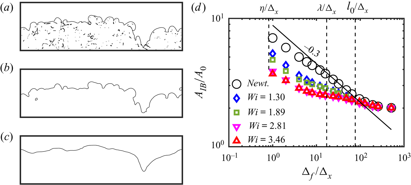
In order to respond to this question (prompted by an anonymous referee) we have carried out here a similar investigation as described in de Silva et al. (Reference de Silva, Philip, Chauhan, Meneveau and Marusic2013), Mistry et al. (Reference Mistry, Philip, Dawson and Marusic2017) and Krug et al. (Reference Krug, Holzner, Marusic and Reeuwijk2017). Indeed, the viscoelastic IB should be a fractal just like the IBs from Newtonian fluids (de Silva et al. Reference de Silva, Philip, Chauhan, Meneveau and Marusic2013), where the surface areas measured at the Kolmogorov and integral scales are related by
 \begin{equation} A_{\eta} = A_l (\eta/l)^{2-D_f}, \end{equation}
where (for Newtonian fluids)  $D_f \approx 7/3$ is the fractal dimension (Sreenivasan Reference Sreenivasan1991; de Silva et al. Reference de Silva, Philip, Chauhan, Meneveau and Marusic2013).
In the present work we have made use of the so-called ‘filtering method’ to determine the fractal dimension of the IB (de Silva et al. Reference de Silva, Philip, Chauhan, Meneveau and Marusic2013; Krug et al. Reference Krug, Holzner, Marusic and Reeuwijk2017; Mistry et al. Reference Mistry, Philip, Dawson and Marusic2017). The procedure starts with the application of a 3-D box filter to the vorticity magnitude field used to detect the IB surfaces as described in § 3.1. Figure 13(a–c) shows a single line from the upper IB corresponding to the Newtonian case (no filtering), together with the IBs obtained after the application of a box filter with sizes  $\Delta _f/\Delta _x = 8$ and
 $64$. As expected the filtering operation has a smoothing effect on the IB which is similar to what is observed in similar curves obtained in numerical and experimental works e.g. de Silva et al. (Reference de Silva, Philip, Chauhan, Meneveau and Marusic2013) and Krug et al. (Reference Krug, Holzner, Marusic and Reeuwijk2017).
(a–c) A single line of the upper IB for the Newtonian case in a fixed spanwise plane ( $z$) and showing entire extent in the
 $x$ direction (
 $L_x$) (a), followed by the same curve obtained after filtering the vorticity magnitude with a box filter with
 $\Delta _f/\Delta _x = 8$ and
 $64$ (b,c) respectively. Bubbles and islands are removed from the curves prior to the computation of the total surface area of each IB. (d) Fractal characteristics of the IB for the present DNS of Newtonian and viscoelastic fluid obtained with the ‘filtering method’ (de Silva et al. Reference de Silva, Philip, Chauhan, Meneveau and Marusic2013; Krug et al. Reference Krug, Holzner, Marusic and Reeuwijk2017; Mistry et al. Reference Mistry, Philip, Dawson and Marusic2017; Balamurugan et al. Reference Balamurugan, Rodda, Philip and Mandal2020). Here,
 $A_{IB}$ is the total area of the (upper and lower) IB surfaces and
 $A_0 = L_x \times L_z$ is a reference area. The filter size
 $\Delta _f$ is normalised by the grid size
 $\Delta _x$ and the figure shows results (for all the simulations) for filter sizes equal to
 $\Delta _f / \Delta _x =$ 2, 4, 6, 8, 12, 16, 24, 32, 48, 64, 96, 128, 192 and 256. The vertical lines show the locations of the Kolmogorov, Taylor and integral scales (these values are taken from the Newtonian reference simulation). The fractal dimension is obtained from the exponent of the power laws computed with the points between the Taylor and integral scales. The solid dark line has a slope of
 $-0.3$ which corresponds to a fractal dimension of
 $D_f = 2.3$ for the surface defining the IB in the Newtonian case. Smaller values of the fractal dimension are recovered for the viscoelastic cases.

The second step consists in computing the slope of the curves of  $A_{IB} = A_{IB} (\Delta _f)$, where
 $A_{IB}$ is the area of the IB surface as shown in figure 13(d). It is crucial that this slope is computed between appropriate ‘inner’ and ‘outer’ scales of motion, because the fractal characteristics of turbulence are not observed near the Kolmogorov and integral scales of motion (de Silva et al. Reference de Silva, Philip, Chauhan, Meneveau and Marusic2013; Krug et al. Reference Krug, Holzner, Marusic and Reeuwijk2017; Mistry et al. Reference Mistry, Philip, Dawson and Marusic2017; Balamurugan et al. Reference Balamurugan, Rodda, Philip and Mandal2020). As in, e.g. Balamurugan et al. (Reference Balamurugan, Rodda, Philip and Mandal2020), we have selected the Taylor (
 $\lambda$) and integral
 $l_0$ scales of motion as ‘inner’ and ‘outer’ scales, respectively. It is clear that in all cases a power law
 $A_{IB} \sim \Delta _f^{-\alpha }$ is observed. For the Newtonian case we get
 $\alpha \approx 0.30$ and from (6.5) we have
 $2-D_f = - \alpha$ so that the fractal dimension (for the Newtonian case) can be estimated to be
 $D_f \approx 2.30$, which is very close to the values of
 $D_f \approx 2.3-2.4$ obtained in the literature e.g. de Silva et al. (Reference de Silva, Philip, Chauhan, Meneveau and Marusic2013).
Figure 13(d) shows also the fractal dimension corresponding to the viscoelastic cases. It is clear that the fractal dimension decreases as the Weissenberg number increases, and we get  $\alpha = 0.14, 0.15, 0.08$ and
 $0.06$ for the viscoelastic simulations with
 $Wi=1.30, 1.89, 2,81$ and
 $3.46$, respectively, which correspond to the fractal dimensions of these surfaces being equal to
 $D_f = 2.14, 2.15, 2.08$ and
 $2.06$. Interestingly, the value of
 $D_f$ seems to be reaching the limit of
 $D_f \approx 2$ i.e. the surfaces become almost regular i.e. non-fractal for very high values of the Weissenberg number. This result is similar to what is observed in stably stratified flows where the entrainment rate decreases (compared with non-stratified flows) because of a strong decrease of the interface area (Reeuwijk, Krug & Holzner Reference Reeuwijk, Krug and Holzner2018).
Thus the strong decrease of the surface area of the IB observed in viscoelastic flows shown in table 3, which ultimately explains their diminished entrainment rate, is caused by a decrease in the ‘roughness’ of the IB surface, consistent with a depletion of the scales of motion imprinted on the IB.
In order to observe the local entrainment velocity figure 14 shows the surface of the IB, coloured by the instantaneous (local) values of the entrainment velocity, for all the simulations of the present work. It is clear that for the Newtonian case negative values of  $v_n$ are preferentially associated with the crests of the IB surface, while positive values emerge from the throughs. This agrees again with the findings of Wolf et al. (Reference Wolf, Luthi, Holzner, Krug and Kinzelbach2012) and Watanabe et al. (Reference Watanabe, Sakai, Nagata, Ito and Hayase2015) for a Newtonian fluid. Moreover, the regions with
 $v_n<0$ appear to be slightly more frequent than the regions of
 $v_n>0$, which is also consistent with the mean values of
 $\left \langle v_n \right \rangle <0$ shown in table 3. The effect of increasing
 $Wi$ for the viscoelastic cases can be also appreciated in these figures. As
 $Wi$ increases the “roughness” of the IB decreases, and this leads to a simultaneous decrease of the magnitude of the surface area, and also a decrease of the frequency of the regions with
 $v_n >0$, which explains therefore why the mean value of
 $\left \langle - v_n \right \rangle$ augments with
 $Wi$.
Top view of the iso-surfaces of the IB – obtained using the selected vorticity magnitude threshold – for all the simulations carried out in the present work: (a) Newtonian; (b)  $Wi=1.30$; (c)
 $Wi=1.89$; (d)
 $Wi=2.81$; (e)
 $Wi=3.46$. The IB is coloured by the magnitude of the entrainment velocity
 $v_{n}$. Negative values mean that the fluid at the IB is moving into the irrotational flow region.

For the range of  $Wi$ used in the present work, although the entrainment rate decreases when increasing
 $Wi$, it is clear that the entrainment velocity steadily increases with
 $Wi$. It is therefore important to investigate more in detail the contribution for this fact arising from the several terms in (6.4).
Table 4 lists the mean values of the entrainment velocity  $v_n$ (same as in table 3) decomposed into its several contributions defined in (6.4). For the Newtonian case and, in agreement with Watanabe et al. (Reference Watanabe, Sakai, Nagata, Ito and Hayase2014), the mean values of the two viscous contributions
 $\left \langle V_D \right \rangle$ and
 $\left \langle V_{\varepsilon } \right \rangle$ are the highest but nearly cancel as they are being approximately symmetric (
 $\left \langle V_D \right \rangle \approx - \left \langle V_{\varepsilon } \right \rangle$), so that mean vortex stretching contribution
 $\left \langle V_P \right \rangle$ becomes important in determining
 $\left \langle v_n \right \rangle$. A similar cancelation somehow exists also in the viscoelastic cases, but the viscoelastic contribution (
 $V_V$) increases with the Weissenberg number and becomes by far the most important contribution to the entrainment velocity for higher
 $Wi$.
Mean entrainment velocity  $\left \langle - v_{n} \right \rangle$ decomposed into its several contributions defined in (6.4), computed at the IB, for all the simulations used in the present work. Negative values mean that the fluid at the IB is moving into the irrotational flow region.

In order to understand the interplay between the several terms as the Weissenberg number increases we need to look into the p.d.f.s of all the contributions to the entrainment velocity, which are shown in figure 15 for the Newtonian case (figure 15a) and for the simulations with the lowest (figure 15b,c) and highest Weissenberg numbers (figure 15d,e).
The p.d.f.s of the entrainment velocity  $v_n$, and of its several contributions defined in (6.4) computed at the IB: (a) Newtonian; (b)
 $Wi=1.30$; (c)
 $Wi=1.89$; (d)
 $Wi=2.81$; (e)
 $Wi=3.46$. Negative values mean that the fluid at the IB is moving into the irrotational flow region.

It is clear that the local values of the enstrophy production term ( $V_P$) are always very small compared with the other terms. This is not surprising because
 $v_n$ is computed using the terms from (6.4) computed at the IB where the enstrophy production is negligible i.e.
 $P_{\varOmega } \approx 0$ and therefore
 $V_P \approx 0$. On the other hand the magnitude of the local viscoelastic contribution (
 $V_V$) increases with
 $Wi$. For the highest
 $Wi$ number cases the p.d.f. of the entrainment velocity seems to collapse onto the p.d.f. of the viscoelastic contribution (figure 15d,e), which suggests that in this case the entrainment velocity is effectively imposed by the viscoelastic contribution. It is also clear that the increase of the Weissenberg number is concomitant with a general decrease of the local values of the viscous contributions
 $V_D$ and
 $V_{\varepsilon }$.
The analysis of several j.p.d.f.s between the several contributions of (6.4) allow us to shed some light into the interplay between these terms in imposing the entrainment velocity. Figure 16 shows the j.p.d.f.s between the entrainment velocity  $v_n$ and its contributions (production –
 $V_P$, diffusion –
 $V_D$, dissipation –
 $V_{\varepsilon }$, viscoelastic
 $V_V$) for the case with
 $Wi=3.46$. Surprisingly, these j.p.d.f.s are very similar for all the cases (not shown), including the Newtonian case where the last j.p.d.f. does not exist and shows that the contributions from viscous diffusion, production by vortex stretching and viscoelastic production, all exhibit positive correlations with
 $v_n$ for a large range of values of these quantities. Interestingly, the j.p.d.f. for viscoelastic production is remarkably similar to the j.p.d.f. of the production but the j.p.d.f. of these two terms show that they are not correlated (not shown). Numerous other j.p.d.f.s between these terms themselves, and between these terms and the entrainment velocity (not shown) seem to be relatively independent of
 $Wi$ i.e. do not show any dramatic change when moving from the lower to the higher
 $Wi$ cases. This suggests that the observed increase of the entrainment velocity with
 $Wi$, caused by the (increase) of the viscoelastic production is not due to a fundamentally different relation between the several physical mechanisms involved, but rather by the local intensification of the local values of the viscoelastic production, together with a decrease of the local values of the viscous terms and production, observed in figure 15.
The j.p.d.f.s between the entrainment velocity  $v_n$ and several of its contributions for the simulation with
 $Wi=3.46$: (a) enstrophy production contribution
 $V_P$, (b) enstrophy diffusion contribution
 $V_D$, (c) enstrophy dissipation contribution
 $V_{\varepsilon }$, (d) viscoelastic production contribution
 $V_V$.

To summarise, although viscoelasticity increases the entrainment velocity with  $Wi$, through the local intensification of viscoelastic production,
 $V_V$, and local reduction of the viscous and vortex stretching terms, it has an even greater impact on the surface area of the IB, leading to a reduction of the entrainment rate. In contrast to classical (Newtonian) fully developed turbulence where IB typically exhibits a fractal character which explains the important transfers of mass, momentum and scalars that take place across turbulent fluid interfaces, in viscoelastic flows the fractal dimension of the IB is strongly attenuated, which leads to the reduction of the effective surface area and thus of the entrainment rate.
We end this section with a couple of remarks that are important to bear in mind when considering (4.1) and (6.4) simultaneously, in any future analysis similar to the ones carried out in the present work. At first sight one may be tempted to infer that the relations between the individual terms discussed in connection to the analysis of (4.1) are similar to the relations observed (for the same terms) in connection to (6.4). After all one can write for instance that  $V_{D} = D_{\varOmega } / | \boldsymbol {\nabla } (\omega _i \omega _i / 2) |$ and
 $v_n = T_{\varOmega } / | \boldsymbol {\nabla } (\omega _i \omega _i / 2) |$ and thus it is normal to expect the relation between
 $D_{\varOmega }$ and
 $T_{\varOmega }$ in connection to (4.1) to be similar to the relation between
 $V_{D}$ and
 $v_n$ in (6.4). This reasoning cannot be made, however, because, whereas (4.1) makes sense in the entire flow domain, (6.4), is designed to compute the entrainment velocity solely at the IB. In other words, whereas the discussion of the individual terms in (4.1) was carried out in the entire flow domain, the analysis of the terms in (6.4) described above relates to their behaviour at the IB only. It is important to clarify this point because important differences arise in the flow dynamics between locations as closely spaced as the IB and the VSL. To illustrate this point figure 17(a,b) shows the j.p.d.f.s between the enstrophy production (
 $P_{\varOmega }$) and enstrophy diffusion (
 $D_{\varOmega }$) for the simulation with
 $Wi=3.46$ at the IB and at the VSL, respectively. It is clear that the two plots are very different. Whereas at the IB no correlation between the two terms can be observed, in the VSL the two terms already display a positive correlation. Many other similar examples could be shown exhibiting similar differences.
The j.p.d.f.s between the enstrophy production ( $P_{\varOmega }$) and enstrophy diffusion (
 $D_{\varOmega }$) for the simulation with
 $Wi=3.46$ at two closely spaced locations: (a) IB; (b) VSL.

7. Conclusions
Numerous experimental results and recent numerical simulations noted that turbulent viscoelastic free-shear flows display a substantial decrease of the entrainment rates compared with the classical values observed for Newtonian fluids. The present work uses several DNS of SFT, i.e. turbulent fronts evolving in the absence of mean shear, in order to address the small scale mechanisms associated with the TE mechanism in viscoelastic fluids.
The simulations use the FENE-P model and rely on pseudo-spectral schemes for spatial discretisation, and in the algorithm proposed by Vaithianathan et al. (Reference Vaithianathan, Robert, Brasseur and Collins2006) which is based on the Kurganov–Tadmor method, to handle the conformation tensor governing equations. The simulations are based on the biggest simulations of forced isotropic turbulence (FHIT) using the FENE-P model yet published, where the Weissenberg and turbulence Reynolds numbers vary in the ranges  $1.30 \le Wi \le 3.46$ and
 $206 \le Re_{\lambda }^{0} \le 404$, respectively. The SFT are started with the FHIT simulations by employing a procedure previously used in several works, as described in Silva et al. (Reference Silva, Zecchetto and da Silva2018), that creates a turbulent front evolving ahead of a turbulent region, in the absence of mean shear, with Reynolds numbers varying in the range
 $98 \le Re_{\lambda } \le 192$ at the time instant used in the subsequent analysis. A reference Newtonian simulation is also carried out using the same procedure, to allow a comparison with the several viscoelastic cases.
The IB is detected using an analysis of the volume of the turbulent region as a function of the vorticity magnitude threshold, described and used in numerous works, and, for the reference Newtonian simulation, exhibits the characteristic large number of crests and troughs, spanning a wide range of scales, characteristic of a fractal surface, that has been observed in IBs from other Newtonian fluids. For the viscoelastic cases as the Weissenberg number increases the size of the largest scales imprinted on the IB also increases, reflecting the increase of the turbulent integral scale of the flow, but a depletion of the small scale ‘roughness’ of the IB is also observed, which is caused by the increase of the size of the smallest scales of motion within the flow. These two facts explain the strong attenuation of the fractal dimension of the IB observed in the viscoelastic cases.
The conditional mean profiles of the enstrophy governing transport equations in the Newtonian case resemble the ones observed in numerous other works. Specifically, while in the turbulent core region production by vortex stretching is balanced by enstrophy viscous dissipation, within the TNTI layer, at the IB the enstrophy increases initially by viscous diffusion (in the viscous superlayer), and later by enstrophy production by vortex stretching (in the TSL). In the viscoelastic cases a new term – the viscoelastic production – associated with the interaction between the vorticity field and polymer stresses, adds new complexity to the dynamics of the enstrophy within TNTIs for viscoelastic fluids. This term is always positive in the viscous superlayer (including at the IB), and thus contributes to the initial growth of the enstrophy in the TNTI layer. It can be positive or negative in the turbulent core region, depending on the values of the Weissenberg number and becomes as important as the enstrophy production term for the cases with the highest  $Wi$.
The structure of the TNTI layer is equal in the Newtonian and in the viscoelastic cases, comprising a VSL and a TSL i.e. for the range of values of  $Wi$ considered in this work, no new region arises within the TNTI layer (viscoelastic superlayer) due to the interactions between the vorticity and the polymeric stresses. For low and moderate values of
 $Wi$ the sizes of the TNTI layer and of its two sublayers are close to the ones typically observed for Newtonian fluids, however, for high
 $Wi$, the scaling is different, since the Kolmogorov micro-scale is no longer the characteristic length scale of the TNTI layer in these cases.
The entrainment rate was investigated by computing the surface area of the IB and the entrainment velocity. The entrainment velocity increases with the Weissenberg number, but the decisive factor explaining the decreased entrainment rates observed in the viscoelastic cases, compared with the Newtonian case, is the substantial reduction of the surface area of the IB observed to occur as the Weissenberg number increases. This area reduction is explained by a reduced scale separation arising in the fluid solvent as  $Wi$ increases that causes a dramatic decrease of the fractal dimension of the IB.
Acknowledgements
The authors are grateful to Professor K. Horiuti for interesting discussions. We acknowledge PRACE for awarding us access to resource Marenostrum IV based in Spain at https://www.bsc.es. The authors acknowledge Minho Advanced Computing Center for providing HPC computing and consulting resources that have contributed to the research results reported within this paper (https://macc.fccn.pt).
Funding
C.B.S. acknowledges Fundação para a Ciência e Tecnologia (FCT) through IDMEC, under LAETA, project UIDB/50022/2020. F.T.P. is thankful for funding by FCT via project PTDC/EMS- ENE/2390/2014 and by FCT and Centro de Estudos de Fenómenos de Transporte through projects UIDB/00532/2020 and UIDP/00532/2020. H.A. acknowledges the University of Lisbon (UL), Instituto Superior Ténico (IST) and the Mechanical Engineering Institute (IDMEC). C.B.S. acknowledges Fundação para a Ciência e Tecnologia (FCT) through projects PCIF/GFC/0109/2017 and PTDC/CTA-MET/3392/2020.
Declaration of interests
The authors report no conflict of interest.