INTRODUCTION
The East Asian winter monsoon (EAWM), a major component of the Asian climate system, is characterized by prevailing low-level cold and dry northwesterly winds associated with the Siberian–Mongolian High (Ding, Reference Ding1994). The EAWM encompasses a larger meridional domain than the East Asian summer monsoon (EASM), and it transmits climate signals from the high-latitude North Atlantic to mid- and low-latitude regions (Porter and An, Reference Porter and Zhisheng1995; Ding et al., Reference Ding, Rutter, Liu, Sun, Ren, Rokosh and Xiong1998; Oppo and Sun, Reference Oppo and Youbin2005; Nagashima et al., Reference Nagashima, Tada, Tani, Sun, Isozaki, Toyoda and Hasegawa2011), strongly influencing about one-third of the global population (Ding et al., Reference Ding, Liu, Rutter, Yu, Guo and Zhu1995; An, Reference An2000). Therefore, understanding past changes in the EAWM is of broad scientific and socioeconomic importance.
Over the past several decades, changes in the natural variability and dynamics of EAWM intensity have been investigated using paleoclimate proxies recorded in loess deposits (e.g., Ding et al., Reference Ding, Liu, Rutter, Yu, Guo and Zhu1995; Porter and An, Reference Porter and Zhisheng1995; An, Reference An2000; Guo et al., Reference Guo, Peng, Hao, Biscaye, An and Liu2004; Sun et al., Reference Sun, Wang, Liu and Clemens2010; Hao et al., Reference Hao, Wang, Oldfield, Peng, Qin, Song, Xu, Qiao, Bloemendal and Guo2012), marine sediments (e.g., Wang et al., Reference Wang, Sarnthein, Erlenkeuser, Grimalt, Grootes, Heilig, Ivanova, Kienast, Pelejero and Pflaumann1999; de Garidel-Thoron et al., Reference de Garidel-Thoron, Beaufort, Linsley and Dannenmann2001; Tian et al., Reference Tian, Wang, Chen and Cheng2005; Steinke et al., Reference Steinke, Mohtadi, Groeneveld, Lin, Löwemark, Chen and Rendle-Bühring2010; Huang et al., Reference Huang, Tian and Steinke2011), lake sediments (e.g., Yancheva et al., Reference Yancheva, Nowaczyk, Mingram, Dulski, Schettler, Negendank, Liu, Sigman, Peterson and Haug2007; Wang et al., Reference Wang, Lu, Liu, Gu, Mingram, Chu and Li2008, Reference Wang, Li, Lu, Gu, Rioual, Hao and Mackay2012, Reference Wang, Jiang, Jiang, Zou, Liu, Zhang and Hao2018; Jia et al., Reference Jia, Bai, Yang, Xie, Wei, Ouyang, Chu, Liu and Peng2015; Zhang et al., Reference Zhang, Wang, Sun and Shen2016), and peat sequences (e.g., Yu et al., Reference Yu, Zhou, Liu and Kang2011) and by data–model integration studies (e.g., Sun et al., Reference Sun, Clemens, Morrill, Lin, Wang and An2012, Reference Sun, Yin, Crucifix, Clemens, Araya-Melo, Liu and Qiang2019; Li and Morrill, Reference Li and Morrill2015; Zhang et al., Reference Zhang, Jin and Li2015). Despite the resulting advances in our understanding of orbital-scale and millennial-scale EAWM variability, which have confirmed that monsoon changes are sensitive to astronomical and ice-sheet factors (deMenocal and Rind, Reference deMenocal and Rind1993; Ding et al., Reference Ding, Liu, Rutter, Yu, Guo and Zhu1995; Guo et al., Reference Guo, Peng, Hao, Biscaye, An and Liu2004; Sun et al., Reference Sun, Yin, Crucifix, Clemens, Araya-Melo, Liu and Qiang2019), the relative influence of the possible forcing factors remain controversial. They include insolation forcing (e.g., Imbrie et al., Reference Imbrie, Hays, Martinson, McIntyre, Mix, Morley, Pisias, Prell, Shackleton, Berger, Imbrie, Hays, Kukla and Saltzman1984; Ruddiman et al., Reference Ruddiman, Raymo, Martinson, Clement and Backman1989; Shi et al., Reference Shi, Liu, Sun, An, Liu and Kutzbach2011; Sagawa et al., Reference Sagawa, Kuwae, Tsuruoka, Nakamura, Ikehara and Murayama2014; Wen et al., Reference Wen, Liu, Wang, Cheng and Zhu2016), Northern Hemisphere ice-sheet dynamics (e.g., Liu and Ding, Reference Liu and Ding1993, Reference Liu and Ding1998; Ding et al., Reference Ding, Liu, Rutter, Yu, Guo and Zhu1995; Jian et al., Reference Jian, Huang, Kuhnt and Lin2001; Hao et al., Reference Hao, Wang, Oldfield, Peng, Qin, Song, Xu, Qiao, Bloemendal and Guo2012), atmospheric carbon dioxide (CO2) concentrations (e.g., Hori and Ueda, Reference Hori and Ueda2006; Liu et al., Reference Liu, Carlson, He, Brady, Otto-Bliesner, Briegleb and Wehrenberg2012; Jiang and Tian, Reference Jiang and Tian2013), and the Atlantic meridional overturning circulation (AMOC) (e.g., Huang et al., Reference Huang, Tian and Steinke2011; Sun et al., Reference Sun, Clemens, Morrill, Lin, Wang and An2012; Wen et al., Reference Wen, Liu, Wang, Cheng and Zhu2016).
The causes of these diverse interpretations are complex and beyond the varying sensitivities of both models and different proxies to the forcing factors (Ding et al., Reference Ding, Liu, Rutter, Yu, Guo and Zhu1995; Wang et al., Reference Wang, Lu, Liu, Gu, Mingram, Chu and Li2008; Lu et al., Reference Lu, Yi, Liu, Mason, Jiang, Cheng and Stevens2013; Liu et al., Reference Liu, Wen, Brady, Otto-Bliesner, Yu, Lu and Cheng2014). An additional important reason may be the lack of investigations of the driving mechanisms of spatial differences in EAWM variability in China on the orbital timescale, which impedes our understanding of EAWM behavior and the underlying forcing mechanisms. Modern climatological studies on annual to multi-decadal scales (Wang et al., Reference Wang, Wu, Chang, Liu, Li and Zhou2010; Chen et al., Reference Chen, Wu and Chen2014), and studies of the Holocene on centennial and millennial timescales (Zhang et al., Reference Zhang, Jin and Li2015), suggest that EAWM variability varied spatially between its northern and southern modes as a result of different driving mechanisms (Wang et al., Reference Wang, Wu, Chang, Liu, Li and Zhou2010; Chen et al., Reference Chen, Wu and Chen2014; Li and Morrill, Reference Li and Morrill2015; Kim et al., Reference Kim, An, Jun, Park and Yeh2017).
Here we present a new reconstruction of EAWM intensity since the last glacial maximum (LGM) based on the variation of a specific sedimentary grain-size component together with high-precision optically stimulated luminescence (OSL) dating from the southeastern margin of the Chinese Loess Plateau (CLP) in northern China. This new EAWM record from northern China was then compared with a high-resolution and chronologically well-constrained EAWM proxy record from the South China Sea (SCS) to assess the spatial variability of the EAWM on the orbital timescale. The proxy data are also compared with model results from transient simulations of the EAWM since the LGM to evaluate the spatiotemporal characteristics of EAWM evolution. The relative impacts of insolation, ice sheets, and atmospheric CO2 on EAWM variability are then evaluated using sensitivity experiments with the Community Climate System Model 3 (CCSM3). Our objectives were to evaluate spatial differences in EAWM variability throughout China during the last glacial–interglacial transition on the basis of proxy data and model simulations to elucidate the mechanisms driving EAWM variability on orbital timescale.
MATERIALS AND METHODS
Study site
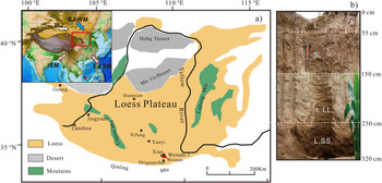
The Weinan loess section (109°34′17.2″E, 34°24′11.3″N, 670 m asl) is located in the central part of a “Yuan” (stable loess tableland) in the southeastern margin of the CLP (Fig. 1a). The section is located far from dust-source regions, and therefore fluctuations in the extent of distant deserts have little impact on the grain size (Smith, Reference Smith1942; Rea, Reference Rea1994; Nugteren and Vandenberghe, Reference Nugteren and Vandenberghe2004; Sun et al., Reference Sun, Chen, Clemens, Liu, Ji and Tada2006), although the grain size of loess in the CLP can be affected by the intensity of the transporting winds (e.g., Liu, Reference Liu1985; Ding et al., Reference Ding, Liu, Rutter, Yu, Guo and Zhu1995; Hao et al., Reference Hao, Wang, Oldfield, Peng, Qin, Song, Xu, Qiao, Bloemendal and Guo2012) and the source-to-sink distance (e.g., Ding et al., Reference Ding, Sun, Rutter, Rokosh and Liu1999; Yang and Ding, Reference Yang and Ding2008). Therefore, the grain-size record from Weinan can be regarded as a reliable proxy of variations in the intensity of the EAWM. The modern mean annual temperature and precipitation at Weinan are 13.6°C and 645 mm, respectively.
(color online) (a) Site location, showing major atmospheric circulation regimes in East Asia and locations of the Gulang, Jingyuan, Huanxian, Xifeng, Xunyi, and Shiguanzhai loess profiles and the record of the sea surface temperature (SST) gradient in the South China Sea. (b) Profile of the sampled loess–paleosol sequence (L0, S0, L1LL1 and L1SS1) at Weinan. EAWM, East Asian winter monsoon; EASM, East Asian summer monsoon; WJ, Westerly jet; ISM, Indian Summer Monsoon.

The studied section is ~3.2 m thick (Fig. 1b) and is composed of loess layer L0 (0–55 cm), the Holocene brownish paleosol S0 (55–150 cm), the last glacial yellowish loess layer L1LL1 (150–250 cm), and the weakly developed paleosol L1SS1 (250–320 cm). The loess (L1)/paleosol (S0) boundary can be identified in the field on the basis of soil color and texture. Bulk samples were collected at a 2 cm interval for grain size and magnetic susceptibility measurements.
Laboratory methods
Grain size and magnetic susceptibility
For grain-size analysis, 0.15 g of sample was first treated with 10 ml of 30% H2O2 and heated to 140°C to remove organic matter (Diao and Wen, Reference Diao and Wen1988; An et al., Reference An, Kukla, Porter and Xiao1991b). After the reaction was completed, the sample was removed from the heat and 10 ml of 10% HCl was added to remove carbonates. Distilled water was then added to reduce the acidity, and the sample was left to stand for 24 h. Subsequently, the supernatant was siphoned off using latex tubing, and the samples were then dispersed for 10 min in an ultrasonic bath with 10 ml 10% (NaPO3)6 solution. Finally, the grain-size distributions were measured using a Coulter LS 13 320 laser grain-size analyzer with a measurement range of 0.375–2000 μm. After oven drying at 40°C, the magnetic susceptibility of the bulk samples (10 g) was measured at a frequency of 0.47 kHz using a Bartington Instruments MS2 meter and MS2B sensor. The samples were measured three times, and the results were averaged.
Numerical partitioning of grain-size components
The grain-size characteristics of sediments are sensitive to changes in transport processes (Visher, Reference Visher1969) and have been widely used to reconstruct the eolian depositional environment, which in northern China is closely related to the EAWM. Significant scientific advances have consequently been made in understanding the long-term behavior of the EAWM (An et al., Reference An, Kukla, Porter and Xiao1991b; Xiao et al., Reference Xiao, Porter, An, Kumai and Yoshikawa1995; Sun et al., Reference Sun, Bloemendal, Rea, Vandenberghe, Jiang, An and Su2002). The sedimentary processes of modern or geological aeolian deposits are usually influenced by multiple transport mechanisms; for example, the median and coarse silt components are transported mainly in short-term suspension mode at low levels in the atmosphere and can therefore be easily trapped by vegetated and moist surfaces and by topographic irregularities (Pye, Reference Pye1987, Reference Pye1995; Tsoar and Pye, Reference Tsoar and Pye1987; Sun et al., Reference Sun, Bloemendal, Rea, Vandenberghe, Jiang, An and Su2002, Reference Sun, An, Su, Lu and Sun2003, Reference Sun, Bloemendal, Rea, An, Vandenberghe, Lu, Su and Liu2004; Qin et al., Reference Qin, Cai and Liu2005). Finer particles are transported in long-term suspension over a larger vertical height range and can be distributed over a large area before deposition, usually by rainfall (Tsoar and Pye, Reference Tsoar and Pye1987). Grain-size components reflect different sediment transport processes, and the components potentially preserve environmental information about these processes. Therefore, grain-size parameters of bulk samples cannot simply be used as environmental indicators in sedimentary sections, and it is necessary to separate specific grain-size components in bulk samples.
In this study, we used the partitioning method of Sun et al. (Reference Sun, Bloemendal, Rea, Vandenberghe, Jiang, An and Su2002) to define various grain-size components in the Weinan section. The method involves fitting a designated distribution function (e.g., the Weibull function) to the measured grain-size data, which enables calculation of the function parameters of the individual grain-size components. The grain-size function of a sample is the sum of all of the individual components, and the mean grain size of individual components can be plotted versus time to provide temporal information about the transport process responsible for each component (Sun et al., Reference Sun, Bloemendal, Rea, Vandenberghe, Jiang, An and Su2002, Reference Sun, An, Su, Lu and Sun2003, Reference Sun, Su, Bloemendal and Lu2008).
Chronology
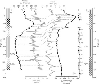
OSL dating allows the direct and accurate determination of the burial ages of lithogenic sediments and has been widely applied to loess-paleosol sequences (e.g., Stevens et al., Reference Stevens, Armitage, Lu and Thomas2006; Stevens and Lu, Reference Stevens and Lu2009; Kang et al., Reference Kang, Lu and Wang2011, Reference Kang, Wang and Lu2013; Marković et al., Reference Marković, Timar-Gabor, Stevens, Hambach, Popov, TomiĆ and Obreht2014). The chronology of the Weinan loess section was established by correlating with the nearby profile with high-resolution (10–20 cm intervals) quartz OSL dating (named Weinan-1) (Kang et al., Reference Kang, Wang and Lu2013), located 2.8 km from our section in the central part of the same Yuan (Fig. 1) and with a very similar sedimentary environment indicated by paleoclimatic proxies (see Fig. 2 and Supplementary Fig. 1).
Records of lithology, magnetic susceptibility, and mean grain-size records and the location of optically stimulated luminescence (OSL) dates for the Weinan (WN) and Weinan-1 (WN-1) sections. The chronology for WN is based on OSL dates from WN-1. (a) Lithology for WN; (b) magnetic susceptibility record for WN; (c) mean grain-size record for WN; (d) mean grain-size record for WN-1 (Kang et al., Reference Kang, Wang and Lu2013); (e) magnetic susceptibility record for WN-1 (Kang et al., Reference Kang, Wang and Lu2013); (f) OSL ages and errors (1σ error bars) for WN-1 (Kang et al., Reference Kang, Wang and Lu2013); (g) lithology for WN-1 (Kang et al., Reference Kang, Wang and Lu2013). Dashed lines link the age control points for WN and WN-1.

The similarity of the OSL ages of the three uppermost L0 samples from Weinan-1 (WN-1, 0 cm; WN-1, 10 cm; and WN-1, 20 cm), with OSL ages of 0.8 ± 0 ka, 0.7 ± 0 ka, 0.6 ± 0 ka, respectively, suggests possible anthropogenic disturbance of the uppermost 20 cm (Kang et al., Reference Kang, Wang and Lu2013). Therefore, these dates were excluded from the final OSL age model for WN-1 (Kang et al., Reference Kang, Wang and Lu2013), and consequently we assigned the age of 0 ka to the uppermost part of L0.
Since the loess-paleosol stratigraphy and variations paleoclimatic proxies (mean grain size and magnetic susceptibility) are correlative between the two sections (Fig. 2), the chronology of the Weinan-1 section can be transferred to the Weinan section. Fourteen chronostratigraphic tie points were selected, including stratigraphic boundaries (i.e., L0/S0 and S0/L1LL1 boundaries), rapid shifts, and the peak of paleoclimatic proxies (MS and MGS). Then the ages of the sampling horizons can be calculated by using a magnetic susceptibility model (Kukla et al., Reference Kukla, Heller, Liu, Xu, Liu and An1988; Kukla and An, Reference Kukla and An1989). Consequently, an independent timescale for the Weinan section for the past 35,000 years was obtained.
The resulting OSL ages of the L0/S0 and S0/L1LL1 boundaries are 4 ka and 13.1 ka, respectively. In addition, 14C dating results suggested that the calendar age of the base of S0 at Weinan is ~12.8 ka (Liu et al., Reference Liu, Chen, Nie, Song, Guo, Li, Gao, Qiao and Ma1994), which is in good agreement with the results obtained from our section. Although this correlated chronology may contain a few errors, we consider it to be acceptable for the analysis of orbital-scale climate changes because the magnetic susceptibility and mean grain-size records from the two sections are comparable.
EAWM proxy record from marine sediments of the SCS
The EAWM influence may extend far toward the equator via the northerly winds over eastern China (Wang et al., Reference Wang, Wu, Chang, Liu, Li and Zhou2010). In this study, a published, well-dated sea surface temperature (SST) gradient index in the SCS (Huang et al., Reference Huang, Tian and Steinke2011) was used for characterizing EAWM variation in southern China. This SST gradient index is derived by subtracting the southwestern SST stack (cores located within the modern “cold tongue” area) from the southeastern SST stack (cores outside the “cold tongue” area), which dominates the region (109–115°E, 5–10°N) in the southern SCS (Fig. 1), using a variety of alkenone-based SST records (Huang et al., Reference Huang, Tian and Steinke2011). The northerly EAWM advects cold and dry continental air to the southwestern SCS along the Vietnam coast, forming a cold tongue and in turn a positive west-to-east SST gradient. A stronger west–east SST gradient is therefore produced by a stronger northerly EAWM (Yu et al., Reference Yu, Huang, Chin, Mii and Chen2006; Tian et al., Reference Tian, Huang and Pak2010; Huang et al., Reference Huang, Tian and Steinke2011). Furthermore, both modern observations for the period of 1948–2009 (Kalnay et al., Reference Kalnay, Kanamitsu, Kistler, Collins, Deaven, Gandin, Iredell, Saha, White, Woollen, Zhu, Leetmaa, Reynolds, Chelliah, Ebisuzaki, Higgins, Janowiak, Mo, Ropelewski, Wang, Jenne and Joseph1996) and the TraCE21 simulation since the LGM (Wen et al., Reference Wen, Liu, Wang, Cheng and Zhu2016) show that the winter west–east SST gradient is in agreement with the winter surface vector wind speed in the SCS, supporting the use of the west–east SST gradient as an index of the EAWM.
EAWM simulations
To investigate the possible forcing mechanisms of EAWM variability, we compared the reconstructions with a transient simulation of climatic evolution of the past 21 ka (TraCE21) (Liu et al., Reference Liu, Otto-Bliesner, He, Brady, Tomas, Clark and Carlson2009, Reference Liu, Wen, Brady, Otto-Bliesner, Yu, Lu and Cheng2014). The TraCE21 simulation was performed using a state-of-the-art coupled ocean–atmosphere model, the CCSM3 of the National Center for Atmospheric Research, with a spatial resolution of T31 (3.75° × 3.75°) (Collins et al., Reference Collins, Bitz, Blackmon, Bonan, Bretherton, Carton, Chang and Doney2006). The full TraCE simulation is forced by realistic external forcing of orbitally induced insolation (ORB) (Berger, Reference Berger1978), atmospheric greenhouse gases (GHGs) (Joos and Spahni, Reference Joos and Spahni2008), meltwater fluxes (MWFs) (Liu et al., Reference Liu, Otto-Bliesner, He, Brady, Tomas, Clark and Carlson2009), and continental ice sheets (ICE) (ICE-5G, Peltier, Reference Peltier2004). TraCE21 is proven to have a reasonable ability to simulate long-term changes in the EASM and EAWM from the LGM onward (Liu et al., Reference Liu, Wen, Brady, Otto-Bliesner, Yu, Lu and Cheng2014; Wen et al., Reference Wen, Liu, Wang, Cheng and Zhu2016). More information about the performance of the CCSM3 model for simulating changes in Asian paleoclimate are detailed in Meehl et al. (Reference Meehl, Arblaster, Lawrence, Seth, Schneider, Kirtman and Min2006) and Otto-Bliesner et al. (Reference Otto-Bliesner, Brady, Clauzet, Tomas, Levis and Kothavala2006).
To explore the relative importance of ORB, glacial factors, and atmospheric CO2 changes in driving orbital-scale EAWM variability, four single-forcing transient simulations (ORB, GHG, ICE, and MWF) were conducted in the same way as the full TraCE simulation, except that each sensitivity experiment was forced by a single forcing with the other transient forcings fixed at the start of each simulation. Simulations ORB and GHG were initialized from the full TraCE state at 22 ka, while simulations ICE and MWF were initialized at the full TraCE state of 19 ka.
In this study, the EAWM index was defined as the area-averaged winter (December–January–February [DJF]) meridional wind in East China (110–120°E, 27–37°N) at the 1000 hPa level. To evaluate spatial differences in the impacts of astronomical, glacial forcing, and CO2, the EAWM index was averaged over northern China (NC, 30–40°N, 110–120°E) and southern China (SC, 20–30°N, 110–130°E). The two regions for definition of southern China and northern China are representative to capture the typical regional differences in EAWM (i.e., Wen et al., Reference Wen, Liu, Wang, Cheng and Zhu2016; Xie et al., Reference Xie, Liu, Chen and Korty2019), although they are not exactly identical to the Weinan profile in the CLP in northern China and the region (5–10°N; 109–115°E) in the southern SCS in reconstruction.
RESULTS
Distribution functions for the grain-size components
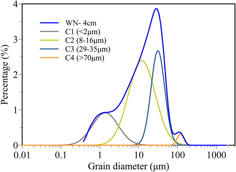
In the case of the Weinan loess samples, partitioning resulted in the clear definition of four grain-size components (Fig. 3). The first component (C1) (modal size <2 μm) probably reflects the influence of chemical or biochemical processes associated with pedogenesis (Paton, Reference Paton1978; Guo et al., Reference Guo, Biscaye, Wei, Chen, Peng and Liu2000, Reference Guo2010). The second component (C2) (modal size 8–16 μm), with a Uf /u* ratio (a suitable criterion for determining the degree of suspension) (Tsoar and Pye, Reference Tsoar and Pye1987) <0.1, is associated with typical windstorms. Dust, once mobilized, can be dispersed across a wide altitudinal range and is transported mainly by upper-level air flow (Pye, Reference Pye1987, Reference Pye1995; Tsoar and Pye, Reference Tsoar and Pye1987; Sun et al., Reference Sun, Bloemendal, Rea, Vandenberghe, Jiang, An and Su2002). The third component (C3) (modal size 29–35 μm), with a Uf /u* ratio in the range of 0.7–0.1, can ascend to a height of several hundred meters (Pye, Reference Pye1987, Reference Pye1995; Tsoar and Pye, Reference Tsoar and Pye1987; Sun et al., Reference Sun, Lu, Rea, Sun and Wu2000). Local surface winds are believed to be the main mechanism of dust transport (Pye, Reference Pye1987, Reference Pye1995; Tsoar and Pye, Reference Tsoar and Pye1987), which in the study area are dominated by the EAWM (An et al., Reference An, Kukla, Porter and Xiao1991a, Reference An, Kukla, Porter and Xiao1991b). Thus, the third component can be used as a proxy index of the intensity of the winter monsoon circulation. The fourth component (C4) (modal size >70 μm) would be able to be suspended for a only very short interval and at very low altitude, even in the case of very strong winds (Pye, Reference Pye1987, Reference Pye1995; Tsoar and Pye, Reference Tsoar and Pye1987).
(color online) Grain-size frequency distribution of a typical sample from Weinan (WN) and its four numerically partitioned components.

Time series of the partitioned grain-size components
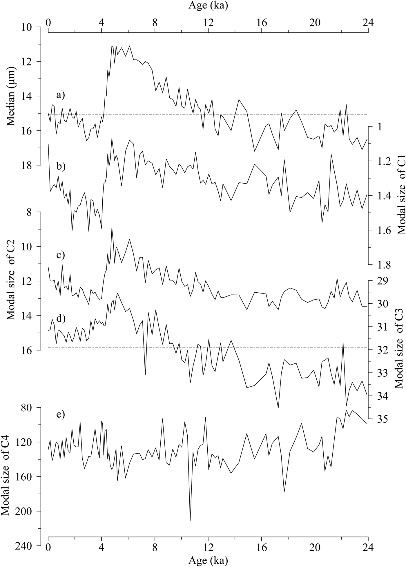
The changes in the extracted grain-size components and median grain size of the Weinan section since the LGM are illustrated in Figure 4. All of the components exhibit a similar pattern of variation, except the fourth component, which has an irregular “saw-tooth” shape and lacks clear long-term trends (Fig. 4e). The first three components exhibit the same pattern of variation as the median grain size, which demonstrates that the grain size was extremely coarse during the LGM, with a maximum during 24–16 ka, gradually becoming finer during 16–8 ka and reaching a trough during 8–4 ka, with a renewed coarsening thereafter. Nevertheless, there is a significant difference between the variation of component 3 (29–35 μm) (C3) (Fig. 4d) and the median grain size (Fig. 4a): the latter has similarly high values during 4–0 ka and the LGM, while the values of C3 are significantly lower during 4–0 ka than at the LGM. As mentioned previously, component C3 is a more reliable proxy of EAWM variations, and it is illustrated in Figures 5b and 6e.
Variations of median grain size and of four numerically partitioned grain-size components from Weinan (WN) since the last glacial maximum (LGM). (a) Median grain size; (b) C1 (grain size <2 μm); (c) C2 (grain size 8–16 μm); (d) C3 (grain size 29–35 μm); (e) C4 (grain size >70 μm). Dashed lines represent the mean values of the median grain size and component C3.

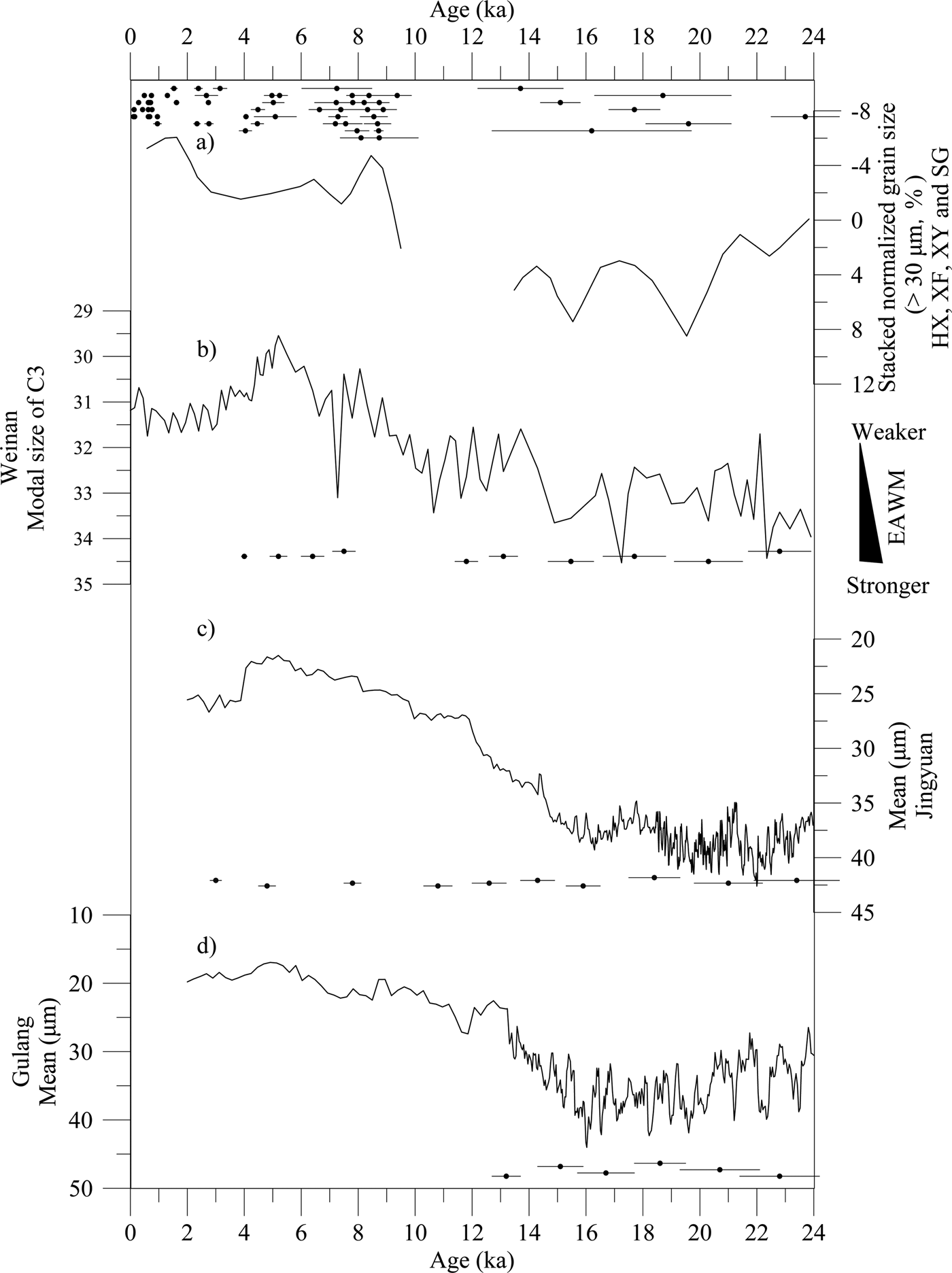
Comparison of various grain-size records of East Asian winter monsoon (EAWM) intensity since the last glacial maximum (LGM). (a) Stacked normalized grain size (% >30 μm) record from the Huanxian (HX), Xifeng (XF), Xunyi (XY), Shiguanzhai (SG) section in the Chinese Loess Plateau (CLP) (Stevens and Lu, Reference Stevens and Lu2009; Lu et al., Reference Lu, Mason, Stevens, Zhou, Yi and Miao2011); (b) record of grain-size component 3 (29–35 μm) from the Weinan (WN) section; (c) mean grain-size record from the Jingyuan section in the western CLP (Sun et al., Reference Sun, Clemens, Morrill, Lin, Wang and An2012); (d) Mean grain-size record from the Gulang section in the western CLP (Sun et al., Reference Sun, Clemens, Morrill, Lin, Wang and An2012). Optically stimulated luminescence (OSL) ages and errors (1σ error bars) for the four sequences are indicated. The locations of the loess profiles are shown in Figure 1.

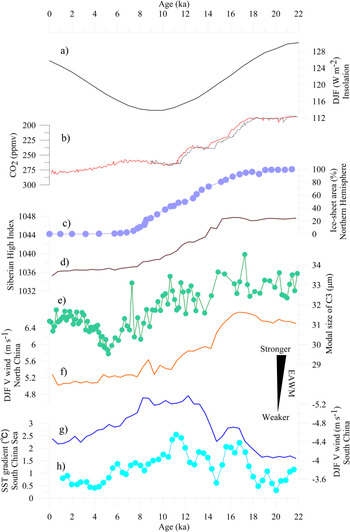
(color online) Response of proxy- and model-derived East Asian winter monsoon (EAWM) changes to insolation, ice sheets, and atmospheric carbon dioxide (CO2) forcing. (a) Winter (December–January–February [DJF]) insolation at 30°N (Berger and Loutre, Reference Berger and Loutre1991); (b) atmospheric CO2 concentration from Dome Concordia, Antarctica (Lüthi et al., Reference Lüthi, Le Floch, Bereiter, Blunier, Barnola, Siegenthaler and Raynaud2008; Parrenin et al., Reference Parrenin, Masson-Delmotte, Köhler, Raynaud, Paillard, Schwander, Barbante, Landais, Wegner and Jouzel2013); (c) Northern Hemisphere ice-sheet area (Dyke, Reference Dyke, Ehlers and Gibbard2004) (right scale); (d) Siberian High Index (SHI) from the TraCE simulation, which was based on the maximum value of sea-level pressure (SLP) in winter (DJF) (Sahsamanoglou et al., Reference Sahsamanoglou, Makrogiannis and Kallimopoulos1991) over the region (40–55°N, 90–120°E); (e) EAWM record based on the variation of grain-size component 3 (29–35 μm) from the Weinan (WN) section in northern China (this study) (right scale); (f) changes in EAWM wind index in northern China in the full TraCE simulation; (g) changes in EAWM wind index in southern China in the full TraCE simulation (right scale); (h) EAWM reconstruction based on alkenone-based west–east SST gradient from the southern South China Sea (SCS) (Huang et al., Reference Huang, Tian and Steinke2011).

The magnetic susceptibility and mean grain size exhibit almost reversal fluctuations at Weinan (Fig. 2). The magnetic susceptibility values of interglacial paleosols are greater than those found in the loess units during the glacial period (Fig. 2). In detail, the magnetic susceptibility gradually increases from L1 to S0, reaching a peak from 8 to 4 ka, followed by a decrease.
Variation of the EAWM between southern and northern China since the LGM
The proxy records demonstrating the spatial pattern of EAWM variability since the LGM are shown in Figure 6. Grain-size component C3 from Weinan indicates a decline in EAWM intensity since the LGM over northern China, reaching a minimum during the period 8–4 ka followed by a renewed increase during the late Holocene (Fig. 6e). The alkenone-based west–east SST gradient in the southern SCS shows that the EAWM intensity over southern China gradually intensified from the LGM into the early Holocene, followed by a weakening in the late Holocene (Fig. 6h). Overall, these trends demonstrate an asynchronous pattern of evolution of the EAWM in northern and southern China since the LGM.
This different pattern of EAWM evolution between southern China and northern China since the LGM (Fig. 6e and h) is reproduced by the TraCE21 simulation (Fig. 6f and g). For northern China, the simulation indicates a continuous decline of the EAWM (Fig. 6f); for southern China, a strengthened EAWM from the LGM to the early Holocene is followed by a subsequent decline (Fig. 6g).
DISCUSSION
Comparison with previous studies of EAWM evolution
In this study, the history of EAWM variability in northern China since the LGM was reconstructed on the basis of numerical partitioning of a loess grain-size record combined with a numerical chronology provided by OSL dating. The results suggest a gradual weakening of the EAWM since the LGM but with an enhancement in the late Holocene (Fig. 5b). In terms of the general trend, the reconstruction is broadly consistent with the TraCE21 simulation on an orbital scale, although it deviated from the simulation during the late Holocene (Fig. 6f). In addition, during the LGM, the stronger-than-present EAWM intensity in northern China (Fig. 6e) was consistent with the multiple Paleoclimate Modelling Intercomparison Project (PMIP) model results (Jiang and Lang, Reference Jiang and Lang2010). This variability of the EAWM is consistent with that indicated by other grain-size records from Chinese loess records in the northern CLP (Lu et al., Reference Lu, Mason, Stevens, Zhou, Yi and Miao2011) (e.g., a normalized grain-size record [>30 μm percentage]) (Fig. 5a) and with the mean grain-size records from the Jingyuan (Fig. 5c) and Gulang (Fig. 5d) sections in the western CLP (Sun et al., Reference Sun, Chen, Clemens, Liu, Ji and Tada2006, Reference Sun, Wang, Liu and Clemens2010; Stevens et al., Reference Stevens, Thomas, Armitage, Lunn and Lu2007; Lu et al., Reference Lu, Mason, Stevens, Zhou, Yi and Miao2011; Sun et al., Reference Sun, Clemens, Morrill, Lin, Wang and An2012; Li and Morrill, Reference Li and Morrill2015). It is also consistent with geochemical records from the Gonghe Basin in the northeastern QTP (Liu et al., Reference Liu, Jin, Sun, Sun and Su2013) and with a record of EAWM intensity based on primary productivity in the Sulu Sea (de Garidel-Thoron et al., Reference de Garidel-Thoron, Beaufort, Linsley and Dannenmann2001).
Note that there is a deviation between the reconstruction and the simulation during the late Holocene. The former indicates a strengthening EAWM, while the latter from TraCE simulation and multiple PMIP models (Tian and Jiang, Reference Tian and Jiang2018) shows a weakening EAWM. The significance of human activity of northern China in the late Holocene (Jing, Reference Jing1991; Dong et al., Reference Dong, Gao and Jin1993; Rhode et al., Reference Rhode, Haiying, Madsen, Xing, Jeffrey Brantingham, Haizhou and Olsen2007; Li et al., Reference Li, Dodson, Zhou and Xinying2009; Schlütz and Lehmkuhl, Reference Schlütz and Lehmkuhl2009; Zhou et al., Reference Zhou, Li, Zhao, Dodson, Sun and Yang2011; Yu et al., Reference Yu, Guo, Wu and Finke2012, Reference Yu, Wu, Finke and Guo2016) can account for the observed deviation. The coarsening of the grain size during the late Holocene in Weinan and other profiles from CLP (Fig. 5) is more likely to reflect a disturbance of the sedimentary record by human activity rather than a genuine strengthening of the EAWM.
However, in southern China, different proxies yield conflicting results regarding the variability of the EAWM, which presents a major challenge for achieving a fundamental understanding of EAWM dynamics. A weakened EAWM from the early to the late Holocene has been suggested by records of diatom assemblages, TOC concentrations, and δ15N from Huguang Maar Lake (Wang et al., Reference Wang, Lu, Liu, Gu, Mingram, Chu and Li2008, Reference Wang, Li, Lu, Gu, Rioual, Hao and Mackay2012; Jia et al., Reference Jia, Bai, Yang, Xie, Wei, Ouyang, Chu, Liu and Peng2015) and by the SST gradient from the southern SCS (Huang et al., Reference Huang, Tian and Steinke2011). By contrast, a high-resolution record of sedimentary Ti concentration from Huguang Maar Lake indicates that the EAWM intensified from the early Holocene to the late Holocene (Yancheva et al., Reference Yancheva, Nowaczyk, Mingram, Dulski, Schettler, Negendank, Liu, Sigman, Peterson and Haug2007). The main cause of these contrasting interpretations of EASM history is the use of ambiguous proxies. In contrast to the SST index in the SCS, which is determined by large-scale dynamics closely related to the EAWM, Lake Huguang Maar is located in a region of complex terrain, and lake sedimentation can be affected by processes within the river's catchment and by various local hydrological processes (Zhou et al., Reference Zhou, Guan and Chi2007; Wen et al., Reference Wen, Liu, Wang, Cheng and Zhu2016). Therefore, the sedimentary Ti record may be linked not only with EAWM intensity but also with the local hydrology. In this regard, the SST gradient is a potentially superior indicator of EAWM variations in southern China because alkenones are considered to record winter SST conditions rather than annual average SST conditions in the SCS (Huang et al., Reference Huang, Wu, Chen, Wang, Tu and Yuan1997; Steinke et al., Reference Steinke, Yu, Kucera and Chen2008).
The EAWM variability indicated by the SST gradient (Fig. 6h) is in agreement with that from the TraCE21 simulation (Fig. 6g) in southern China, which revealed a strengthened EAWM from the LGM to the early Holocene followed by a weakening trend. The stronger- than-present EAWM intensity during the mid-Holocene (Fig. 6g and h) is supported by the results of Tian and Jiang (Reference Tian and Jiang2018) in southern China, whereas the EAWM intensity change, slight or similar to the present (Fig. 6g and h), during the LGM was not exactly identical to the PMIP model results of Jiang and Lang (Reference Jiang and Lang2010).
For the loess grain-size records, individual grain-size components, linked to specific sediment transport processes, can be used to reflect various climatic factors such as the winter monsoon and effective moisture (Tsoar and Pye, Reference Tsoar and Pye1987; Prins et al., Reference Prins, Postma and Weltje2000; Sun et al., Reference Sun, Bloemendal, Rea, Vandenberghe, Jiang, An and Su2002; Xiao et al., Reference Xiao, Li, Jiang, Li, Huang and Xu2005). Therefore, it is important to separate different components in bulk samples and to use specific components for reconstructing changes in the EAWM. In this study, the C3 component (29–35 μm), which is closely related to the EAWM, was selected to indicate EAWM variability. The resulting EAWM record, combined with that of the SST gradient in the southern SCS and the proxy-model comparison, suggests a pronounced spatial difference in EAWM variability between northern and southern China on the orbital scale (Fig. 6e–h). This suggests a weakened EAWM since the LGM in northern China but a strengthened EAWM from the LGM to the early Holocene, followed by a weakening trend, in southern China.
Possible forcing mechanisms of EAWM variability
The difference in the orbital-scale evolution of the EAWM between southern and northern China indicated by both geological records and a TraCE21 simulation likely implies the operation of different forcing factors. Past investigations of the natural variability and forcing of the EAWM based on various geological records (e.g., Porter and An, Reference Porter and Zhisheng1995; An, Reference An2000; de Garidel-Thoron et al., Reference de Garidel-Thoron, Beaufort, Linsley and Dannenmann2001; Tian et al., Reference Tian, Wang, Chen and Cheng2005; Wang et al., Reference Wang, Lu, Liu, Gu, Mingram, Chu and Li2008; Steinke et al., Reference Steinke, Mohtadi, Groeneveld, Lin, Löwemark, Chen and Rendle-Bühring2010; Sun et al., Reference Sun, Wang, Liu and Clemens2010; Huang et al., Reference Huang, Tian and Steinke2011; Chu et al., Reference Chu, Sun, Zhu, Shan, Shang, Ling, Su, Xie, Wang and Liu2017) and paleoclimate models (Zhou and Zhao, Reference Zhou and Zhao2009; Jiang and Lang, Reference Jiang and Lang2010; Shi et al., Reference Shi, Liu, Sun, An, Liu and Kutzbach2011; Wen et al., Reference Wen, Liu, Wang, Cheng and Zhu2016; Xie et al., Reference Xie, Liu, Chen and Korty2019), as well as data–model integration studies (Sun et al., Reference Sun, Clemens, Morrill, Lin, Wang and An2012; Li and Morril, Reference Li and Morrill2015; Zhang et al., Reference Zhang, Jin and Li2015), have significantly improved our understanding of the EAWM. However, the dominant driver of the orbital-scale variations of the EAWM remains unclear due to the varying sensitivity of both proxies and models to the potential forcings, which include insolation (e.g., Imbrie et al., Reference Imbrie, Hays, Martinson, McIntyre, Mix, Morley, Pisias, Prell, Shackleton, Berger, Imbrie, Hays, Kukla and Saltzman1984; Ruddiman et al., Reference Ruddiman, Raymo, Martinson, Clement and Backman1989; Shi et al., Reference Shi, Liu, Sun, An, Liu and Kutzbach2011; Sagawa et al., Reference Sagawa, Kuwae, Tsuruoka, Nakamura, Ikehara and Murayama2014; Wen et al., Reference Wen, Liu, Wang, Cheng and Zhu2016), Northern Hemisphere ice sheets (e.g., Liu and Ding, Reference Liu and Ding1993,1998; Ding et al., Reference Ding, Liu, Rutter, Yu, Guo and Zhu1995; Jian et al., Reference Jian, Huang, Kuhnt and Lin2001; Hao et al., Reference Hao, Wang, Oldfield, Peng, Qin, Song, Xu, Qiao, Bloemendal and Guo2012), atmospheric CO2 (Hori and Ueda, Reference Hori and Ueda2006; Liu et al., Reference Liu, Carlson, He, Brady, Otto-Bliesner, Briegleb and Wehrenberg2012; Jiang and Tian, Reference Jiang and Tian2013), and the AMOC (e.g., Huang et al., Reference Huang, Tian and Steinke2011; Sun et al., Reference Sun, Clemens, Morrill, Lin, Wang and An2012; Wen et al., Reference Wen, Liu, Wang, Cheng and Zhu2016).
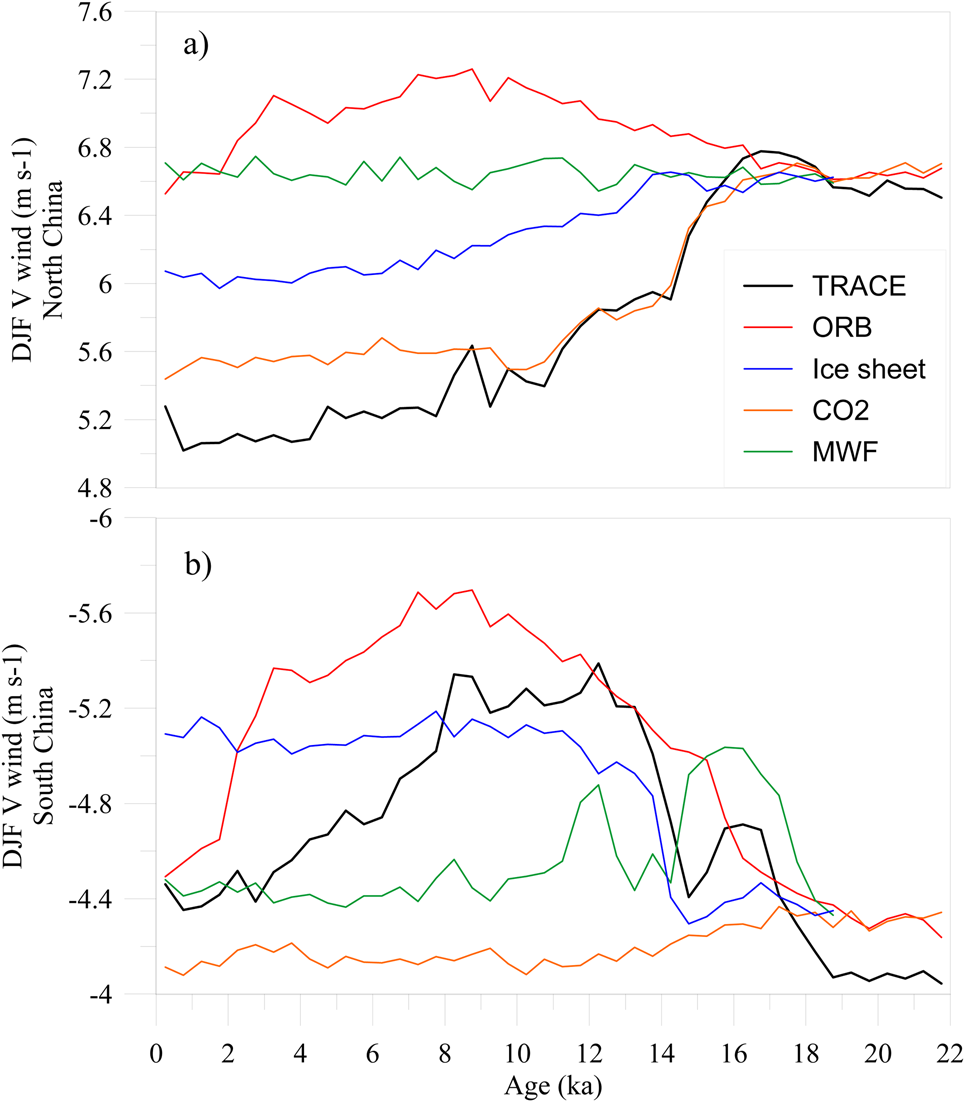
In this study, the TraCE21 simulation of EAWM evolution agrees with the reconstructed EAWM variability in both northern (Fig. 6e and f) and southern China (Fig. 6g and h). It is clear that the weakening trend of the EAWM in northern China (Fig. 6e) is in accordance with the persistent increase in CO2 concentration (Fig. 6b) and the reduction in Northern Hemisphere ice sheets (Fig. 6c). Furthermore, forcing of the northern EAWM by CO2 concentration and ice sheets is supported by the comparison of the full-forcing run with the single-forcing sensitivity experiments (Fig. 7a), which suggests that the EAWM in northern China weakened since the LGM, mainly due to the effects of changes in CO2 concentrations and ice sheets. The impact of diminished ice sheets and increased CO2 would have substantially warmed northern high latitudes (Braconnot et al., Reference Braconnot, Otto-Bliesner, Harrison, Joussaume, Peterchmitt, Abe-Ouchi, Crucifix, Driesschaert, Fichefet, Hewitt, Kageyama, Kitoh, Laîné, Loutre, Marti, Merkel, Ramstein, Valdes, Weber and Zhao2007; Yanase and Abe-Ouchi, Reference Yanase and Abe-Ouchi2007; Liu et al., Reference Liu, Otto-Bliesner, He, Brady, Tomas, Clark and Carlson2009, Reference Liu, Carlson, He, Brady, Otto-Bliesner, Briegleb and Wehrenberg2012; Jiang et al., Reference Jiang, Lang, Tian and Guo2011) and thus decreased the meridional (latitudinal) temperature gradient, which greatly weakened the Siberian High and thus the EAWM (Kutzbach et al., Reference Kutzbach, Guetter, Behling, Selin and Wright1993; Ding et al., Reference Ding, Yu, Rutter and Liu1994; Ding and Yu, Reference Ding and Yu1995; Chen and Huang, Reference Chen and Huang1998; Ruddiman, Reference Ruddiman2008; Hao et al., Reference Hao, Wang, Oldfield, Peng, Qin, Song, Xu, Qiao, Bloemendal and Guo2012).
(color online) Modeled East Asian winter monsoon (EAWM) index for northern China (a) and southern China (b) in full and single forcing experiments from the TraCE21 simulation. Full TraCE simulation (labeled “TRACE”) with changes in transient forcing by insolation, greenhouse gases (GHGs), ice sheets, and meltwater fluxes (MWFs); ORB (only insolation forcing); ice sheet (only ice-sheet forcing); CO2 (only GHG forcing); MWF (only MWF forcing). DJF, December–January–February.

By contrast, in southern China, the reconstructed EAWM based on the SST gradient in the southern SCS (Fig. 6h) varies broadly in concert with changes in insolation (Fig. 6a) and ice sheets before ~8 ka (Fig. 6c). The model results from the single-forcing and full-forcing experiments of the TraCE21 simulation confirm the strong influence of insolation and global ice volume on EAWM variability in southern China (Fig. 7b). It is suggested that ORB changes in the Northern Hemisphere were responsible for the changes in zonal land–sea thermal contrast and thus the sea-level pressure gradient between the ocean and the Asian continent, thereby driving the variability of the EAWM on the orbital scale (Kutzbach, Reference Kutzbach1981; Kutzbach and Guetter, Reference Kutzbach and Guetter1986; Li and Morill, Reference Li and Morrill2015; Wen et al., Reference Wen, Liu, Wang, Cheng and Zhu2016; Xie et al., Reference Xie, Liu, Chen and Korty2019).
The difference in the pattern of evolution of the EAWM between southern and northern China, and the different corresponding forcing mechanisms, reveal the spatially inhomogeneity of EAWM dynamics, which is determined by geographical location and the characteristics of the large-scale atmospheric circulation. For southern China, located in low latitudes and relatively close to the sea, the EAWM circulation is dominated by the land–sea thermal contrast, which is sensitive to changes in insolation (Kutzbach and Guetter, Reference Kutzbach and Guetter1986). However, over northern China, which is much further from the sea, the EAWM circulation is strongly affected by the intensity of the Siberian High in winter, which is sensitive to changes in CO2 concentration and ice sheets via their impact on the meridional temperature gradient. During the last deglaciation, the large fluctuations of the AMOC also significantly affected the intensity of EAWM over northern China (e.g., Huang et al., Reference Huang, Tian and Steinke2011; Sun et al., Reference Sun, Clemens, Morrill, Lin, Wang and An2012; Wen et al., Reference Wen, Liu, Wang, Cheng and Zhu2016).
These different patterns of EAWM evolution between northern and southern China are consistently manifested in geological records and model simulations. Furthermore, the corresponding mechanisms underlying this spatial divergence are also revealed by the sensitivity experiments accompanying the TraCE21 simulation. That is, changes in ice sheets and CO2 concentration dominated the evolution of the EAWM over northern China, while changes in insolation dominated its evolution over southern China. Therefore, the impact on the EAWM of a specific external forcing, such as ice sheets, CO2 concentration, and insolation, was spatially inhomogeneous.
CONCLUSIONS
We have used high-resolution proxy records and TraCE21 climate simulations to investigate the spatially divergent pattern of EAWM evolution since the LGM on the orbital timescale. The results indicate a general weakening of the EAWM since the LGM in northern China but a strengthening of the EAWM from the LGM to the early Holocene, followed by a weakening trend, in southern China. Sensitivity experiments with the TraCE21 simulation indicate that the evolution of the EAWM in northern China was driven mainly by variations in atmospheric CO2 and Northern Hemisphere ice sheets, whereas orbitally driven insolation and ice sheets, especially the former, were the major drivers in southern China. Our results provide improved knowledge of orbital-scale EAWM variability and its forcing mechanisms, especially with regard to spatial differences, which may help understand the response of the East Asian monsoon system to global climate changes in the past and future.
ACKNOWLEDGMENTS
This study was supported by the Strategic Priority Research Program of the Chinese Academy of Sciences (grant XDA13010106, XDB26020503), the National Key Research and Development Program of China (grant 2016YFA0600504), and the National Natural Science Foundation of China (NSFC) (grants 41888101, 41502177, 41690110).
SUPPLEMENTARY MATERIAL
The supplementary material for this article can be found at https://doi.org/10.1017/qua.2020.101