

Introduction
Peter Townsend, best known for his work on poverty and for setting up the Child Poverty Action Group, was one of Britain’s most celebrated twentieth-century social scientists (Renwick, Reference Renwick2023). Townsend defined poverty as relative deprivation, which viewed it as falling seriously below the common or customary living standards of a particular society at a particular time, and he was the first to suggest measuring poverty with a line ‘at, say, 50 per cent or 66 per cent of the [national] average’ (Townsend, Reference Townsend1962, p. 222). His landmark 1968/69 study included an income poverty line set at ‘50 per cent of the [UK] mean’ (Townsend, Reference Townsend1979, p. 248), and it pioneered another measure that was based on ‘deprivation indicators’, such as having no fresh meat most days of the week. Both of Townsend’s poverty measurement ideas are widely used today, albeit after amendments made them more reflective of public experience. While the now conventional ‘60 per cent of median income’ poverty line is often located at about the same income level as Townsend’s ‘50 per cent of mean’ measureFootnote 1 , it is more closely connected to an income people usually experience, as median income is unaffected by the tiny minority of extremely high incomes. Mack and Lansley’s (Reference Mack and Lansley1985) now widely used ‘consensual deprivation’ method has deprivation indicators like Townsend’s, but it incorporates public attitudes and preferences; for possessions and activities to be included they must be classed as ‘necessities’ by at least 50 per cent of survey respondents, and, building on Piachaud’s (Reference Piachaud2010 [Reference Piachaud1981]) landmark critique of Townsend’s (Reference Townsend1979) major work, if a respondent lacks a ‘necessity’ through choice this is not counted as deprivation. These amended versions of Townsend’s income and deprivation measures comprise the present UK government’s strategy to track its progress in reducing child poverty; ‘overall poverty’, the main metric, includes all those in households living on under 60 per cent of median income, while ‘deep material poverty’ consists of those lacking at least four of thirteen items deemed ‘essential’ by majorities of Family Resources Survey respondents (HM Government, 2025a).
It is noteworthy that both Townsend’s response to Piachaud (Townsend, Reference Townsend2010 [Reference Townsend1981]) and his review of Mack and Lansley’s (Reference Mack and Lansley1985) book (Townsend, Reference Townsend1985) argued powerfully against incorporating the public’s attitudes and choices into poverty measurement. Advocating the ‘pursuit of objective social science’, he disregarded the ‘indoctrinated’ public’s feelings and consumer decisions because they are manifestations of prevailing norms and standards in the society being studied (Townsend, Reference Townsend2010 [Reference Townsend1981], p. 234). Detachedly observing social patterns could, he believed, advance poverty measurement by replacing arbitrary lines, such as his ‘50 per cent of mean income’ measure, with a scientifically meaningful one. When interviewed later in life he described the goal of achieving such a meaningful cut-off point separating the poor from the non-poor as ‘extraordinarily important’; using the importance of ‘Geiger counters’ in identifying dangerous levels of radiation as an example, Townsend asserted that ‘the idea of a threshold is dominant in science’, and so therefore ‘poverty is a phenomenon which can only be regarded as scientific if we’re talking about a level of income and other resources where it really matters whether you have a certain amount or a higher amount’ (see Thompson, Reference Thompson2019). His attempt to find such a level was based on a ‘deprivation index’ that simply counted how many of a selected twelve ‘deprivation indicators’ his 1968/69 respondents lacked; the twelve are highlighted with an asterisk [*] in this article’s Appendix, which lists all sixty. Townsend (Reference Townsend and Townsend1970) believed he would find a point in the income distribution below which scores on his index would increase at a faster rate as income fell, and that the poverty line should be placed at this income ‘threshold’. After his major study’s publication (Townsend, Reference Townsend1979) the existence or otherwise of this threshold was ‘hotly debated’ (Nolan and Whelan, Reference Nolan and Whelan1996, p. 63). Townsend (Reference Townsend1979, p. 255) initially stated that the evidence is ‘inconclusive, but suggests that such a threshold may exist’. However, he later claimed (Townsend, Reference Townsend and Townsend1993, p. 56) its existence had been confirmed by a ‘more sophisticated analysis of the same evidence’ carried out by Desai (Reference Desai and Golding1986) and Desai and Shah (Reference Desai and Shah1988). Gordon (Reference Gordon, Bradshaw and Sainsbury2000, p. 41) drew the same conclusion, but other senior academics have disputed the claim (examples include Glennerster, Reference Glennerster2011, Hirsch et al., Reference Hirsch, Padley, Stone and Valadez-Martinez2020).
The research presented in this article casts new light on the threshold controversy in two ways. Firstly, it uses all sixty of Townsend’s deprivation indicators; computer-based data analysis was far more time-consuming in the 1970s, and Townsend later reflected that it was a ‘pity’ he and his research team had not included more of the sixty in their analysis, as doing so would be ‘a better basis for the [measurement] of poverty’ (quoted in Thompson, Reference Thompson2019). Secondly, the research is informed by key insights from critics of the methods used by Townsend and others to establish the ‘threshold’.
The next part of this article revisits the controversy surrounding Townsend and others’ claim of a poverty ‘threshold’ – i.e. an income level below which deprivation index scores increase more rapidly. It explores the theoretical basis for assuming such a threshold will or will not exist, before examining the threshold’s empirical record. Findings from a new analysis of Townsend’s data, which featured both his approach and one informed by his critics, are then presented. A conclusion reflects on how these empirical findings sit with points made by Townsend and his critics, and what lessons they might hold for contemporary poverty research.
The debate about Townsend’s poverty ‘threshold’
Theoretical issues
In a paper he first presented in 1967, Townsend revealed that his ‘research team are experimenting with a ‘deprivation’ index, based on a list of activities and customs which are common for a majority of the population of the United Kingdom’ and that ‘we assume…there will be a ‘threshold’ of resources below which deprivation will be marked’ (Townsend, Reference Townsend and Townsend1970, p. 29). He did not indicate why his team assumed this. Indeed, considering the subsequent controversy surrounding the ‘threshold’, it is remarkable how little space has been devoted to explaining why it might be expected to exist. Townsend appeared to offer an explanation in his response to Piachaud (Reference Piachaud2010 [Reference Piachaud1981]) when he wrote that ‘with diminishing income, people restrict the nature of, say, a summer holiday, but below some level of income decide to not have a holiday at all’ (Townsend, Reference Townsend2010 [Reference Townsend1981], p. 236). In his example, neither middle/higher class people nor those on working-class incomes that just enable them to afford the cheapest holiday would add to their ‘deprivation index’ score, whereas those below that income level would add one to theirs. Thus, a faster increase in deprivation would exist below the threshold-level income, as the cheapest versions of various necessities became unaffordable more rapidly in relation to falling income.
Piachaud (Reference Piachaud2010 [Reference Piachaud1981, pp. 231–232]) had argued that because ‘poverty is relative’ and there is ‘diversity’ in ‘styles of living’, Townsend’s ‘hypothesis that such a threshold would exist is intrinsically implausible’. His insistence that there is a ‘continuum from great wealth to chronic poverty’ (op. cit., p. 231) had echoes of the lauded statistician and poverty researcher Arthur Bowley’s (Reference Bowley1915, p. 170) assertion that there ‘cannot be any such division [between poor and non-poor] except an arbitrary one, for every quantity involved varies continuously from grade to grade’. Other critics of Townsend highlighted the disjuncture between deprivation and income. In an article best known for casting income-based poverty lines as merely ‘indirect’ measures of poverty, Ringen (Reference Ringen1988, p. 363) stated that ‘since income (as we are able to measure it) is such a poor indicator of consumption, the existence of such a threshold should not be expected’. Indeed, those identified as ‘poor’ by deprivation-based measures and income-based ones differ considerably (Bradshaw and Finch, Reference Bradshaw and Finch2003). Recent UK evidence suggests that income remains a poor indicator of actual deprivation. For example, in 2023/24, of the 2 million children in ‘deep material poverty’ according to the UK government’s deprivation measure, 0.9 million (nearly half) were not among the 4.5 million (31 per cent) in income-based ‘overall poverty’ (HM Government, 2025b, p. 12). Current income is a poor predictor of deprivation because deprivation levels are also affected by accumulated wealth (including savings), gifts, loans, debt repayments, diverse consumer behaviour and living costs being higher in some regions and for some groups, notably disabled people (see Berthoud & Bryan, Reference Berthoud and Bryan2011; Nolan & Whelan, Reference Nolan and Whelan1996; Ringen, Reference Ringen1988). Townsend’s 1968/69 dataset provides a striking example of the relationship between low income and deprivation being potentially impacted by another variable; the over-65s had over three times more savings than respondents in general (a mean of £53.97, compared with £17.11), yet 40.2 per cent of them were below the now conventional ‘60 per cent of median household income’ poverty line, compared to just 13.9 per cent of all respondentsFootnote 2 .
Perhaps surprisingly, Townsend did not discuss the possible effect of any other variable on the relationship between deprivation and income. Indeed, apart from his holiday example and a similar one about Christmas celebrations (see Townsend, Reference Townsend1979, p. 249), neither of which Piachaud (Reference Piachaud1987) or anyone else responded to, Townsend never argued back against those who questioned the theoretical basis of his threshold. Thus, the debate about whether a threshold should be expected to exist was noticeably limited.
Empirical issues
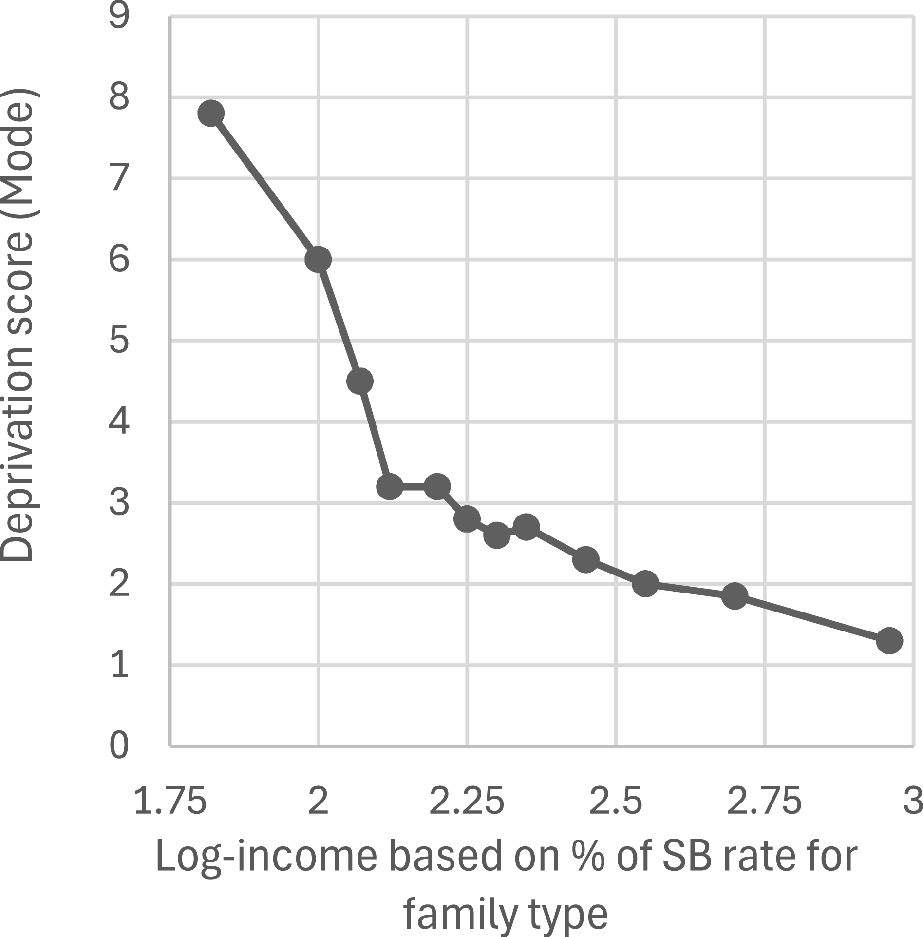
Townsend’s (Reference Townsend1979, p. 261) evidence for a threshold was presented in an often-reproduced graph (including by Piachaud, Reference Piachaud2010 [Reference Piachaud1981], p. 230) that plotted log-transformed income against the ‘mode’ deprivation scores for various income levels. Townsend had standardised income for different family sizes and types by calculating it as a percentage of what the family would receive if it was entitled to Supplementary Benefit (from hereon SB), the main 1960s UK means-tested state benefit. The graph featured an arrow marked ‘140 per cent’ that indicated the threshold’s position, at 140 per cent of SB rates. The coordinates shown in Figure 1 are taken from measuring an enlarged version of Townsend’s (Reference Townsend1979, p. 261) graph. While its gradient clearly changes at around the fourth point from the left, Nolan and Whelan (Reference Nolan and Whelan1996, p. 64) observed that criticisms centred on Townsend’s ‘use of both modal values and a logarithmic income score’ being ‘questionable’ and him applying ‘no statistical tests’ to establish the threshold’s existence.
Threshold graph plotted with points from Townsend’s graph (Reference Townsend1979, p. 261).

Mansfield (Reference Mansfield1986) criticised Townsend’s unexplained and unusual decision to use a mode deprivation score (i.e. the most frequent deprivation score among those in a particular income range) rather than a mean one (whereby deprivation scores in each income range are aggregated and then divided by the number of respondents in that range). He accused Townsend of pursuing a ‘tortuous itinerary’ (Mansfield, Reference Mansfield1986, p. 54) to show that widespread poverty was scientifically proven to exist. Agreeing with Ashton (Reference Ashton1984), he pointed to Abel-Smith and Townsend’s (Reference Abel-Smith and Townsend1965) earlier study, in which they set a poverty line at an arbitrary 140 per cent of means-tested benefit level ‘to produce the shock-figure of 10.1 per cent ‘poverty”’ (Mansfield, Reference Mansfield1986, p. 50). Indeed, as Kincaid (Reference Kincaid1975, p. 179) observed nearer the time, their rejection of a more conventional (at that time) state benefit level poverty line in favour of one ‘40 per cent’ higher delivered an ‘almost fourfold’ increase in the poverty rate. Mansfield (Reference Mansfield1986) suggested Townsend (Reference Townsend1979) had favoured the mode over the mean purely because the former showed a much faster increase in deprivation below his preferred 140 per cent of SB ‘threshold’ level. Townsend did not counter Mansfield’s points. Nor did he comment on whether a threshold would still be visible if modes had been calculated for income ranges that were equal distances apart, unlike the twelve in his analysis (see Townsend, Reference Townsend1979, p. 1001).
Townsend did not explain why he log-transformed his income data, despite it being usual for researchers to justify such decisions. For example, the present author provided a rationale for log-transforming an outcome variable with the natural logarithm ‘Ln’; doing so enabled the inclusion of all cases in a regression analysis without distortions caused by outliers (see Dunn, Reference Dunn2025). While Desai’s (Reference Desai and Golding1986) analysis of Townsend’s (Reference Townsend1979) data used the same log-transformed SB-based income measure without explanation, it compared mean deprivation scores above and below 150 per cent of the family’s SB rate. Desai found a statistically significant difference between the two groups, which led him to ‘confirm the existence of a threshold’ (Desai, Reference Desai and Golding1986, p. 18). However, as Piachaud (Reference Piachaud1987) noted, Desai (Reference Desai and Golding1986) did not measure significance levels at any other income cut-off point. Piachaud (Reference Piachaud1987, p. 162) suggested that if Desai had ‘split the data at around 130 per cent of SB level then he would have shown a more marked split between two patterns’. The other study involving Desai that Townsend cited as evidence of a threshold (see Townsend, Reference Townsend and Townsend1993, p. 56) presented no new relevant evidence; its authors merely cited Desai (Reference Desai and Golding1986) to confirm the threshold’s existence (see Desai and Shah, Reference Desai and Shah1988, p. 513).
Drawing on evidence other than his 1968/69 study, Townsend (Reference Townsend, Bradshaw and Sainsbury2000, p. 13) was later confident enough to accuse the World Bank of being in ‘denial’ about the existence of such a threshold. He wrote of the ‘strong empirical support’ (Townsend, Reference Townsend, Bradshaw and Sainsbury2000, p. 12) provided by his own co-authored work (Gordon and Townsend, Reference Gordon and Townsend1990) and by Sandra Hutton (Reference Hutton1991), but a closer look suggests their evidence is unconvincing. Gordon and Townsend (Reference Gordon and Townsend1990) applied discriminant analysis to a 1985/86 London survey to separate the poor from the non-poor at the point at which the two groups’ other characteristics differed most; as it took account of variables other than deprivation and income in determining the threshold’s position, it cannot be considered to have established a relationship between the two variables of interest. Hutton (Reference Hutton1991) analysed Family Expenditure Survey and General Household Survey data. She established a threshold at around 150 per cent of family means-tested benefit entitlement for only one of five family types studied – elderly women living alone; thresholds for the other four were established at income levels above 200 per cent, which few would consider low enough to position a poverty line.
Thus, Townsend claimed there was a poverty threshold without acknowledging limitations in studies he referred to, without responding to some widely known and telling criticisms, and without offering justifications for his more questionable methodological decisions. The research project discussed in the rest of this article was designed with the unanswered criticisms in mind. Statistical tests are applied to Townsend’s data to find out if a threshold exists, using mean (not just mode) measures of central tendency. Income ranges are equal distances apart, and the income measure used in the present UK government’s poverty measurement strategy is employed alongside Townsend’s SB measure. Variables other than income and deprivation are excluded from the analysis when deciding where any potential threshold should be positioned, but they are included when exploring the possibility that ‘third’ variables might account for all or part of any change in the relationship between income and deprivation.
Methods
The ‘Poverty in the United Kingdom’ study covered many localities, and its large sample was well matched to the country’s population (see Land, Reference Land and Townsend1979; Townsend, Reference Townsend1979, pp. 98–100). Those classed by the original research team as having ‘incomplete data’ are excluded from the present analysis, as are cases with a below 90 per cent rate of clear deprived/non-deprived responses on the deprivation measures’ questions, or with missing values on any other variable of interest. This reduced the sample from 6,043 to 4,847 – close to the 4,853 that featured in earlier analyses (see Townsend, Reference Townsend1979, p. 1001; Desai, Reference Desai and Golding1986, p. 11).
To help deliver transparency and thoroughness on a controversial topic, four deprivation indexes (DIs), each featuring a particular combination of the sixty deprivation indicators, are employed. Townsend’s sub-set of twelve indicators (from hereon called DI12) is supplied as an already computed variable in the available datasetFootnote 3 . Food and social events are emphasised more in DI12 than in the other three DIs. The composition of the other DIs reflects a wish to include as many of the sixty as possible while being mindful of the shortcomings of using DIs that do not apply to the whole sample. DI40 includes only the forty that are relevant to all adults. It therefore excludes the six children’s items, one that applies only to married women (number 10, see Appendix), and those that only apply to the employed – the twelve ‘conditions at work’ indicators and the health indicator about sickness absence from employment (number 41). DI46 is the DI40 plus the six children’s deprivation indicators; both are included to balance concerns that DI40 ignores children’s deprivation and that DI46 might inflate the deprivation scores of households with children relative to those without. Finally, for completeness and transparency, DI60 includes all indicators in Townsend’s study, despite it being likely to overemphasise the deprivation of the employed relative to the jobless.
The SB rate household income measure used by Townsend (Reference Townsend1979) and Desai (Reference Desai and Golding1986) comes already calculated in the dataset. Townsend (Reference Townsend1979, pp. 980–81) provided details of what he included as income. Both Townsend’s income measure and the ‘adjusted household income’ (AHI) measure favoured here deducted the already calculated ‘housing cost’ variable from respondents’ past year’s income before adjusting it for household size and type. Like the current UK government’s income poverty calculations, the AHI divides household income after housing costs by the modified Organisation for Economic Co-operation and Development (OECD) equivalence scale, which counts the first adult as one, any additional adults and 15–17 year-olds as 0.5, and under-15 year-olds as 0.3; income calculations in this article use this method, unless it is stated otherwise. While SB rates were determined by politicians, they might have achieved a similar equivalising effect through reflecting, to some extent, different families’/households’ material needs.
Statistical tests seeking possible correlations between income and deprivation focus on the stretch of income from around the average (mean) down to just above the very lowest. The higher limit is due to the researcher’s interest in only sections of society that could reasonably be considered relatively poor and deprived; mean income for the 4,847 was £597.73 (AHI) and 204.72 per cent (of SB), and this study’s higher income limits fall just below these levels. The lower limit is imposed for the same reason given by Berthoud and Bryan (Reference Berthoud and Bryan2011) and Edmiston (Reference Edmiston2022) – that those on the very lowest incomes tend to have surprisingly low deprivation scores, often due to them underreporting their income (see Brewer et al., Reference Brewer, Etheridge and O’Dea2017).
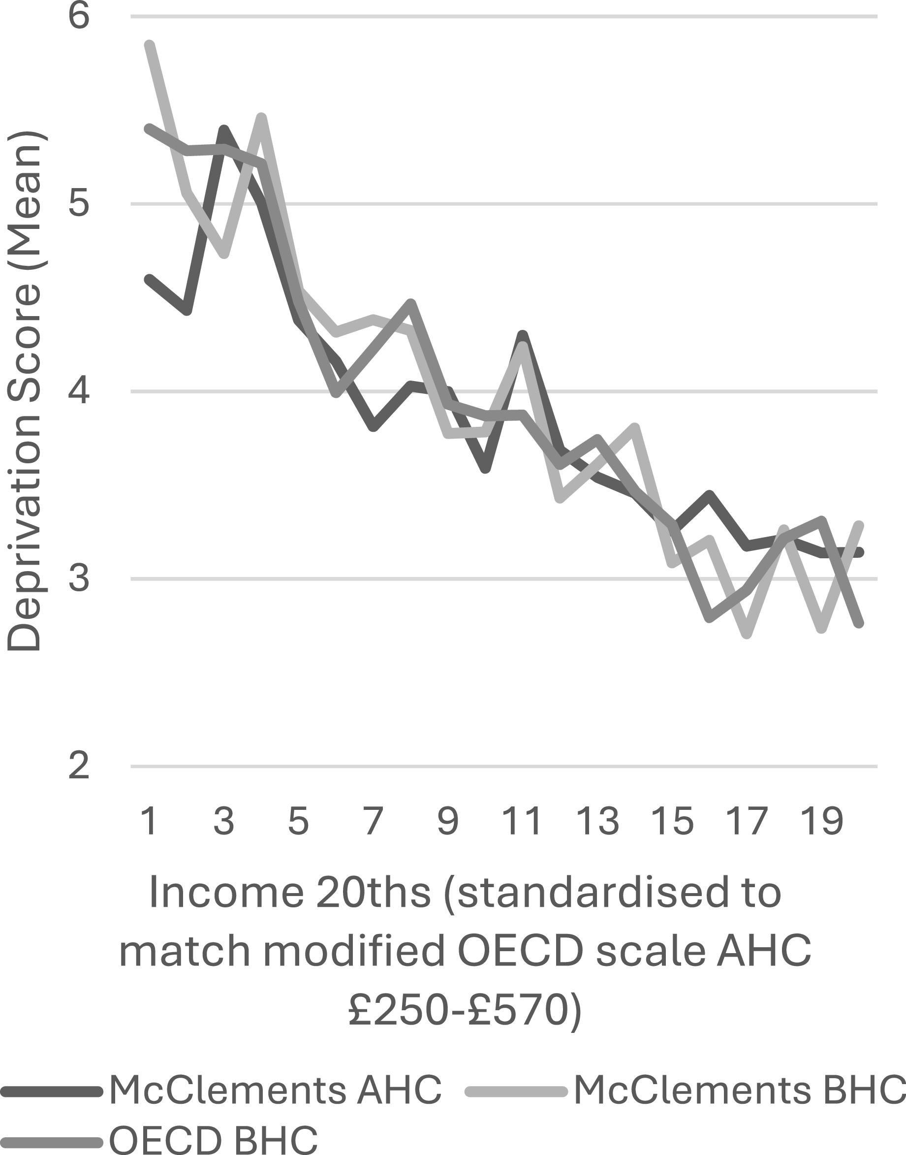
A decision to have numerically convenient cut-off points for twenty levels of income meant that the exact range of incomes differed slightly between the SB and AHI measures. The SB-based measure covered incomes of 100–199 per cent of SB rates, which allowed for twenty income levels each covering 5 per cent; 5.6 per cent of the 4,847 respondents lived on less than 100 per cent of their household’s SB rate, and 39.4 per cent lived on 200 per cent or more, which leaves 2,664 (55.0 per cent) included respondents. For AHI, a range from £250–£569.99 was chosen, with its twentieths covering £16 each; 6.2 per cent of the 4,847 had AHI under £250, while 41.7 per cent had £570 or more, leaving 2,524 (52.1 per cent) included. Cutting income into twentieths enabled statistical comparison of adjacent income groups, and it balanced the need for an acceptable number of measurement points with the need for adequately populated income groups. All SB twentieths contained between 90 and 167 respondents, and all AHI twentieths between 94 and 156. While the ‘mean’ measure of central tendency is used for statistical tests, ‘modes’ and ‘medians’ are included in graphs to enable comparison. To check the findings against other income measures, a limited number of tests used a ‘before’ housing costs (BHC) income measure (not ‘after’ [AHC]) and/or the widely used McClements (Reference McClements1977) equivalence scale; the latter assigns more weight (than the modified OECD scale) to household members other than the first adult. These other income measures were ‘standardised’ by changing them in proportion to the gap between their mean and the AHI’s mean. Standardised incomes were then divided into the same ‘twentieths’ as the AHI, from £250 to £569.99.
To facilitate statistical tests to identify a possible threshold, the following procedure was undertaken. First, ‘Expected DI’ scores were derived. Linear regression equations, in which an income variable predicted deprivation scores across the study’s narrowed income ranges, produced predicted deprivation values for the midpoint of all income ‘twentieths’. DI scores were then standardised by subtracting Expected DI scores from actual DI scores. Cohen’s ‘d’ scores, which are derived from ‘t’ tests for comparing two means, were then used to measure the extent to which standardised DI scores in neighbouring income twentieths differed. If Townsend’s threshold could be said to exist, these Cohen’s ‘d’ scores would be positive and high as income levels decreased below the threshold level. In view of the arbitrary cut-off points in the twenty SB/AHI income categories, if any noteworthy changes in the statistical associations were identified, tests of strength of the deprivation differences either side of more precise income levels were employed to find the optimal cut-off point in the income distribution where a threshold could be positioned.
If any such cut-off point was identified, multivariate analysis would investigate whether the pattern could be wholly or partly accounted for by the role of other variables (such as family forms, age, gender, etc.). This would include logistic regression, as income categories either side of a dividing point can form a dichotomous outcome variable. The relevant DI variable would be included as a predictor, alongside other variables that might help explain any noted shift in the relationship between deprivation and income.
Findings
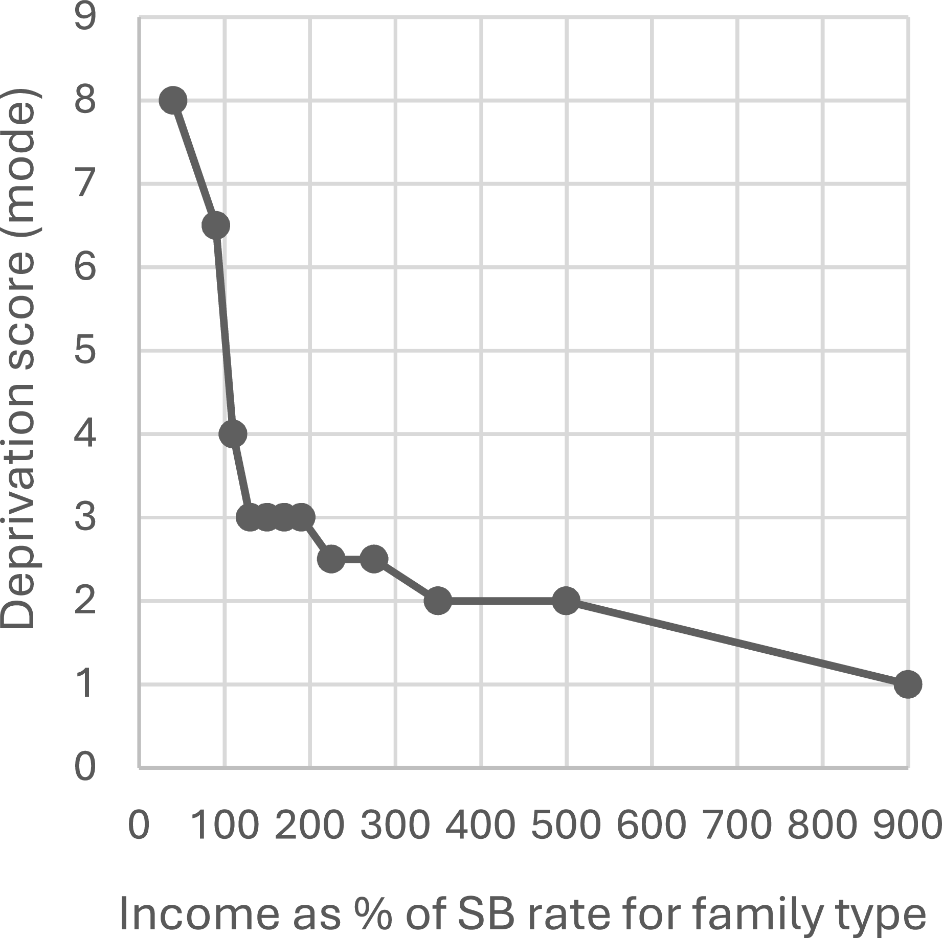
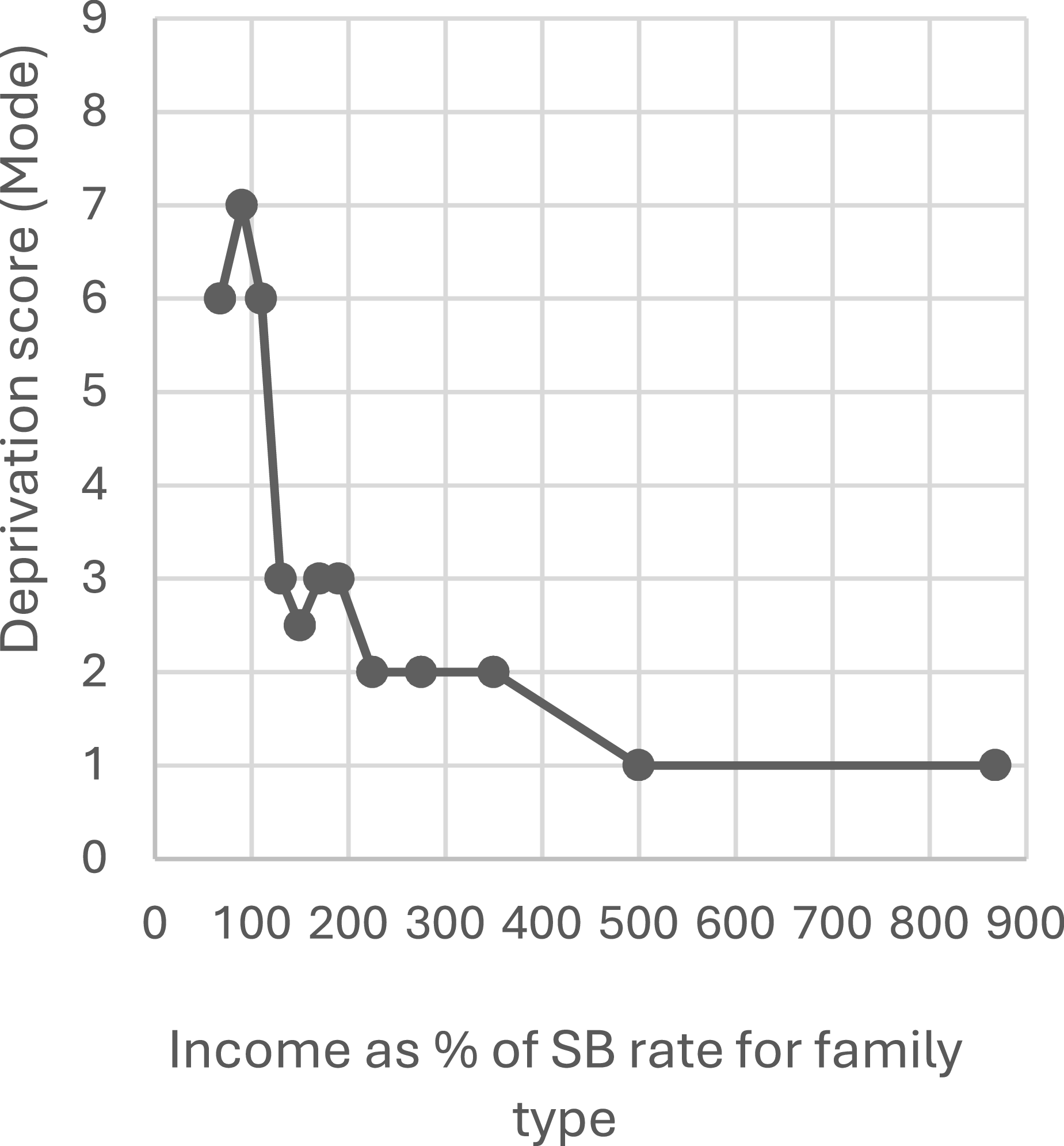
To set the scene and enable comparisons to be made later, Figures 1, 2 and 3 are all versions of the graph Townsend presented when evidencing his poverty ‘threshold’ claim. All three use his ‘modal’ measure of his sub-set of twelve deprivation indicators, and his income measure (a rounded percentage of the family’s SB rate) across his chosen income ranges.
Threshold graph using figures from Townsend (Reference Townsend1979, p. 1001), with income NOT log-transformed.

Threshold graph based on the present author’s analysis of the raw data.

If the log-income scores of between around 1.82 and 2.96 for the twelve points in Figure 1 are considered in connection with corresponding figures tabulated elsewhere (see Townsend, Reference Townsend1979, p. 1001; Desai, Reference Desai and Golding1986, p. 11), it becomes clear that Townsend log-transformed his data with the often-used ‘Lg10’ logarithm. That 1979 graph plotted the tabulated income figures at their mid-points so, for example, the income range of 120–139 per cent of SB rates is at about 2.11 log-income on the x axis, which converts back to 130 per cent of SB rates. Given the nature of modal scores, and the mode figures tabulated by Townsend and Desai, it is surprising that only four of the twelve plotted on Townsend’s graph are integers (i.e. whole/round numbers). With this inaccuracy in mind, Figure 2 uses the tabulated figures. Its income levels are mid-points in the twelve income ranges that Townsend chose to calculate modal scores for, except that the two income ranges at either end (0–79 per cent and >499 per cent of SB) use median incomes, because incomes are far less evenly distributed at these extreme levels.
Figure 2’s similarity to Figure 1 shows that Townsend’s threshold is visible regardless of whether his data is log-transformed. Figure 3 is based on the present author’s analysis using Townsend’s DI12 measure. Its curve is similar to those in Figures 1 and 2, except that modal deprivation drops at the lowest income level (under 80 per cent) to six; it is eight in Townsend (Reference Townsend1979, p. 1001) and Desai’s (Reference Desai and Golding1986, p. 11) tabulated figures. This discrepancy cannot be explained by differences in the composition of reduced samples used by different researchers: of those with less than 80 percent of SB income, sixteen respondents have a DI12 score of six in this reduced (4,847) sample yet there are fewer (fifteen) with a DI12 of eight in the full (6,043) sample. Likewise, it is strange that a mode of 6.5 was calculated for the 80-99 per cent income range, as that range has forty respondents with a DI12 score of seven in the 4,847 sample, while only thirty-four of the 6,043 score six. Importantly, with these recalculated modes, while deprivation leaps as income falls from 130 per cent to 110 per cent of SB, it does not increase more rapidly as income falls to its lowest level; thus, Figure 3 shows that Townsend’s threshold was not established even when all his research decisions were replicated.
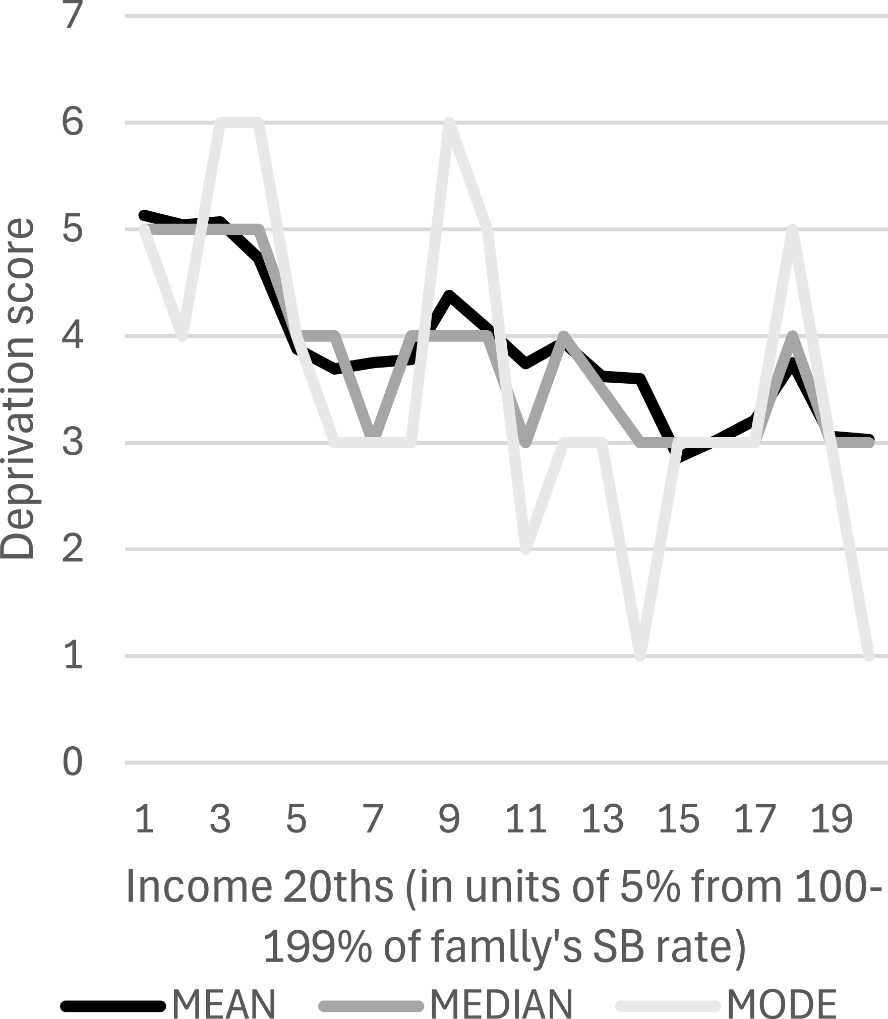
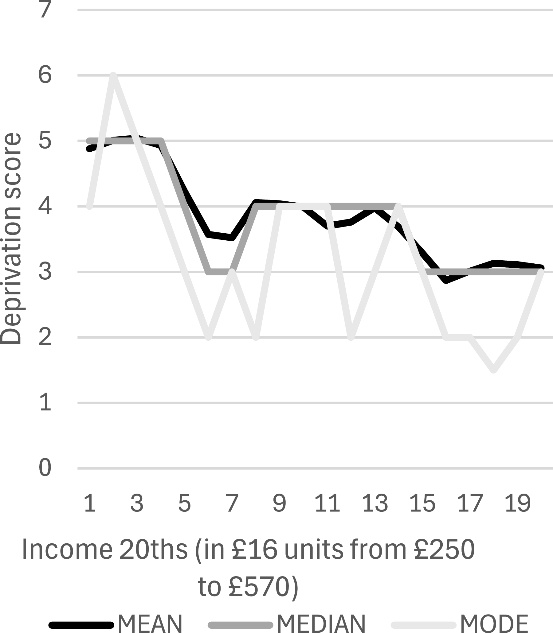
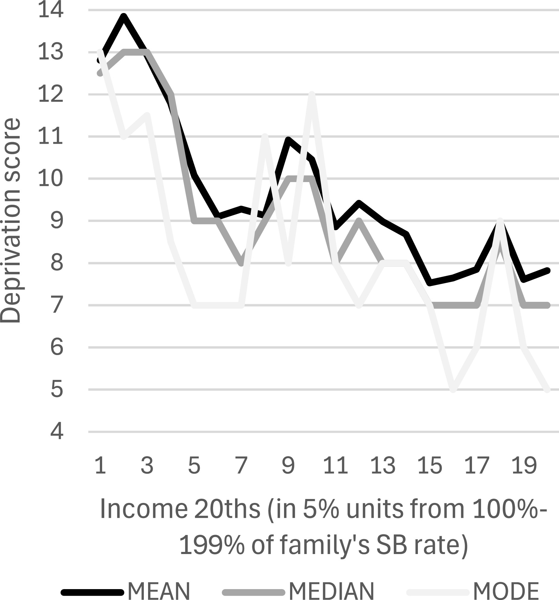
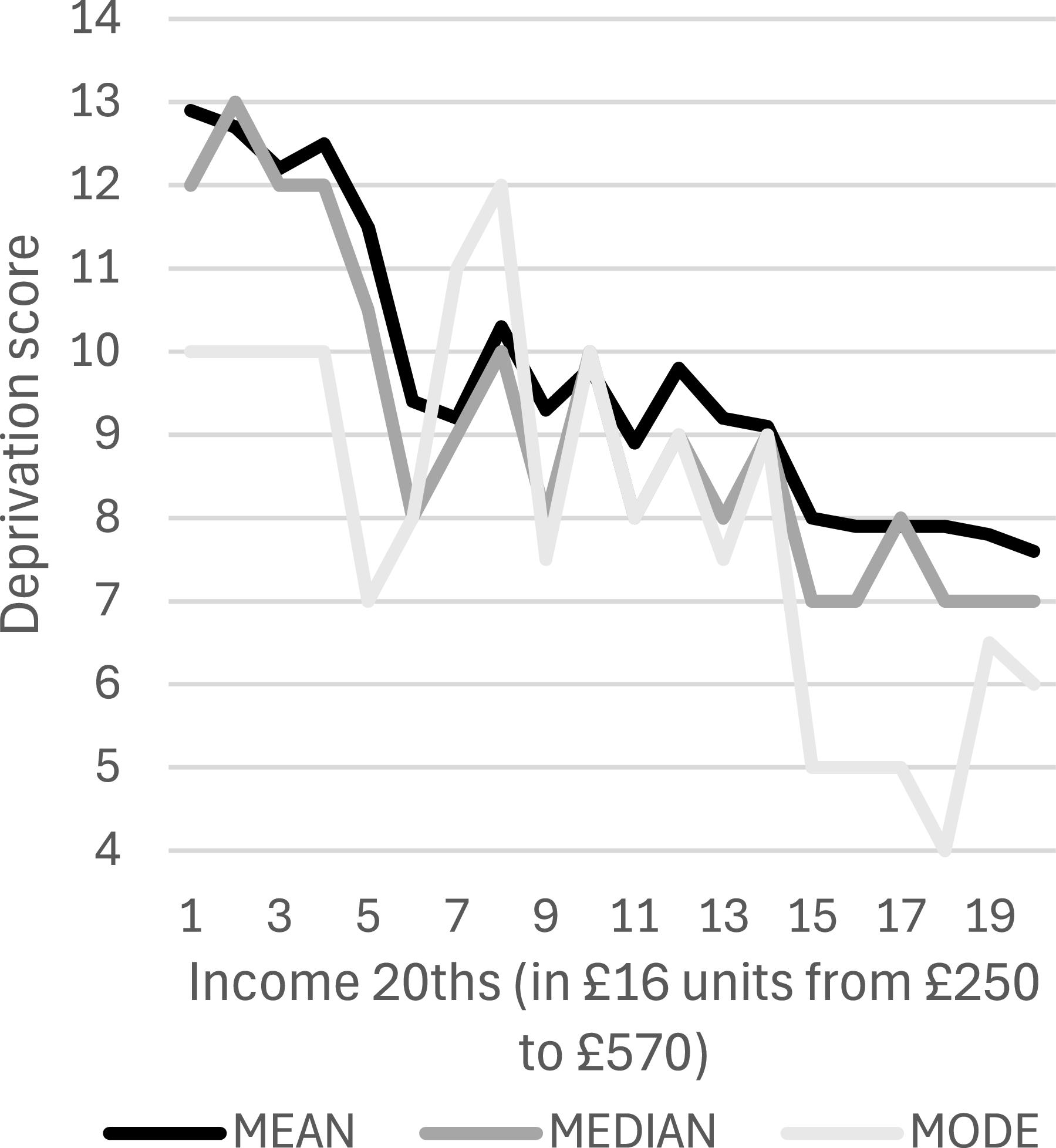
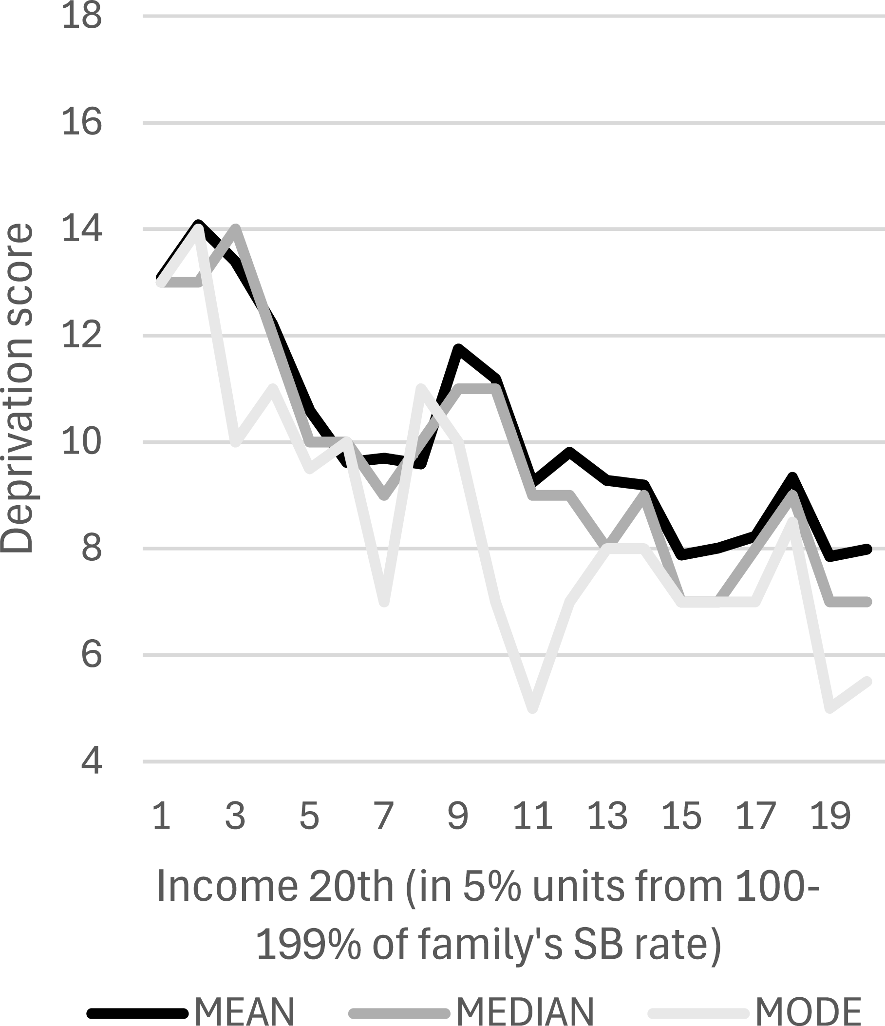
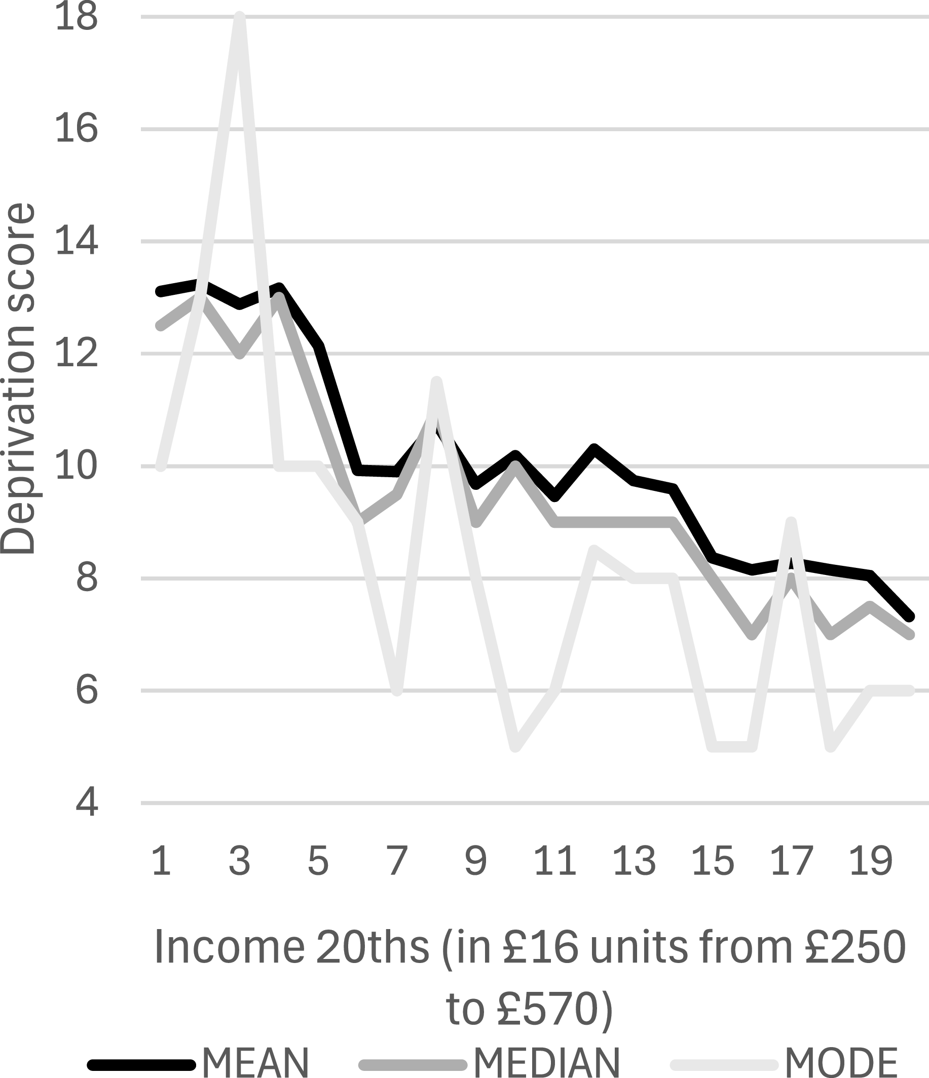
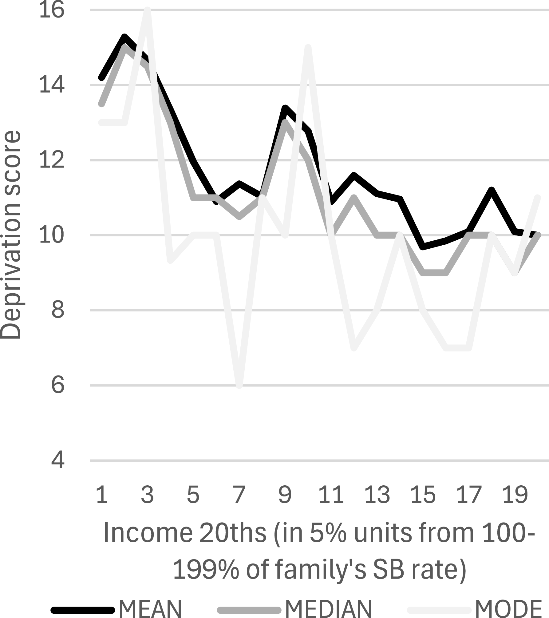
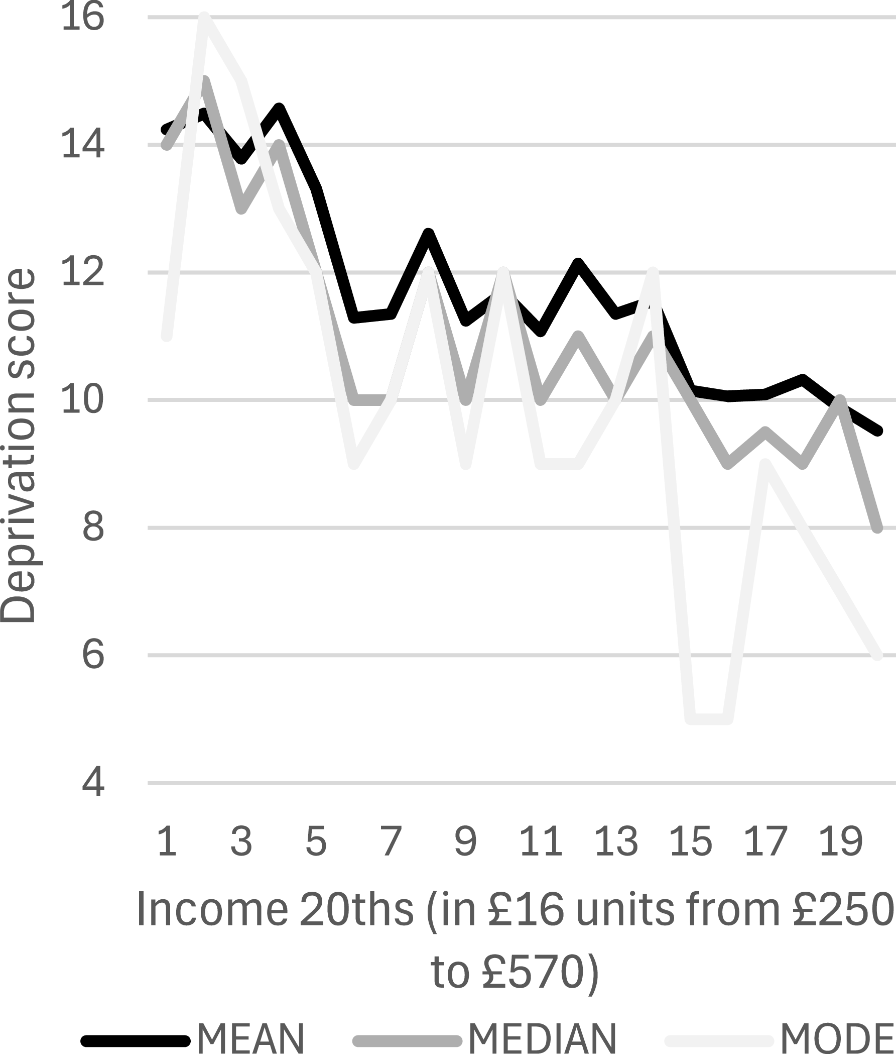
Figures 4–12 present graphs of deprivation and income, using various measures of both. In contrast to Figures 1–3, the gentler gradients in Figures 4–12 indicate how little deprivation levels differ between those at around 45–50 per cent from the top of the income distribution (at the right end of the graphs) and those at around 5 per cent from the bottom (at the left end). For example, Figure 4, which uses Townsend’s DI12, displays the mean (5.13) and median (5) deprivation scores for the lowest SB income category, which are not dramatically higher than those of the highest (3.03 and 3). Indeed, all Pearson’s correlation coefficients for deprivation and income across their entire distributions (not just the part covered by Figures 4–12) are significant but not strong (between −0.27 and −0.37)Footnote 4 .
Income (SB) and Deprivation (Townsend’s DI12).

Income (AHI) and Deprivation (Townsend’s DI12).

Income (Other Measures) and Mean Deprivation (Townsend’s DI12).

Income (SB) and Deprivation (DI40).

Income (AHI) and Deprivation (DI40).

Income (SB) and Deprivation (DI46).

Income (AHI) and Deprivation (DI46).

Income (SB) and Deprivation (DI60).

Income (AHI) and Deprivation (DI60).

There is a stark contrast between the clear change of gradient in Figures 1–3 and the lack of one in Figure 4, despite all four graphs using the same dataset to plot SB income against DI12. Figures 4 and 5 both indicate that even if a mode measure is applied to DI12, but with a different choice of income ranges, no dramatic change in deprivation occurs as income falls. Across all four deprivation measures, the graphs’ mode lines are the most erratic; this is because the presence or absence of just one or two cases can dramatically alter modes, unlike means (if, as in the present analysis, there are no extreme outliers) and medians.
While Figures 4-12 establish no ‘threshold’, they nevertheless show a discernible, though not dramatic, shift upwards in deprivation at around the fourth and fifth AHI income twentieth (covering £298–£345.99) and around the fourth SB twentieth (covering 120–124 per cent). As in Figure 3, though less dramatically, deprivation appears to ‘step up’ after which it appears to plateau as incomes fall further.
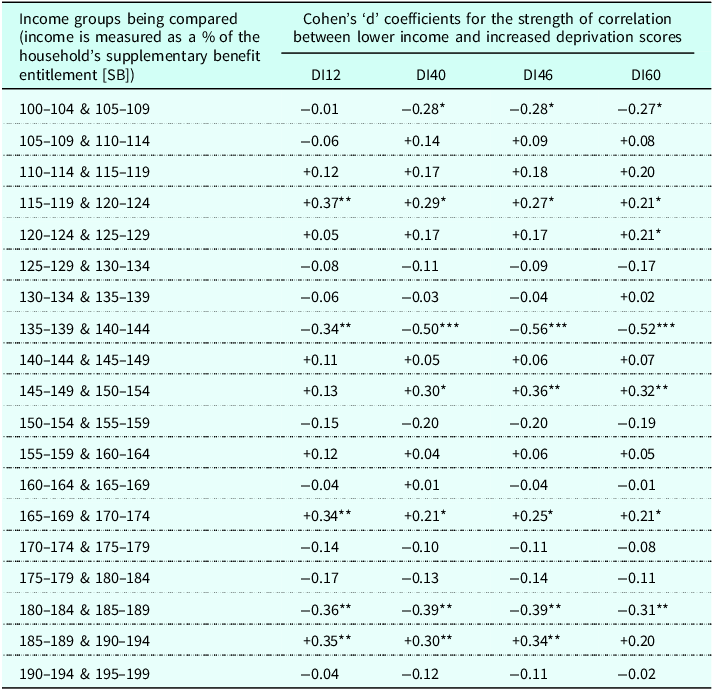
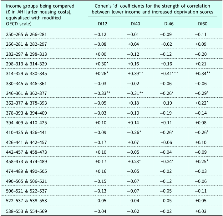
Tables 1 and 2 present findings from statistical tests applied to each of the twenty categories of income and their mean deprivation scores. The tests were to discover whether neighbouring income twentieths differ significantly in deprivation compared to what would be expected if deprivation increased consistently with decreasing income. Table 1 presents findings for the SB income measure; Table 2 presents the AHI findings. A positive (+) score indicates that the lower of two adjacent income categories has higher ‘actual versus expected’ deprivation, while a negative (-) one indicates the opposite. To confirm the existence of a poverty threshold of the kind suggested by Townsend, a consistent pattern of significant, positive correlations across several rows near the top of Tables 1 and 2 is required. No such pattern can be discerned. Instead, there is an uneven mixture of pluses and minuses. Ironically, given Townsend and others’ claims of a threshold at around 140 per cent of SB, across all four measures deprivation decreases significantly in relation to its ‘expected’ trajectory as incomes fall from 140–144 per cent to 135–139 per cent (see Table 1, eighth row down). Indeed, the three strongest correlations in Table 1 are all connected to that drop in deprivation immediately below 140 per cent of SB.
The rate of change in deprivation scores as income (SB) falls

Table 1 Long description
A table comparing income groups and their correlation with deprivation scores using Cohen's d coefficients. The table has 20 rows and 5 columns. The columns are labeled 'Income groups being compared (income is measured as a % of the household's supplementary benefit entitlement [SB])', 'Cohen's d coefficients for the strength of correlation between lower income and increased deprivation scores', 'DI12', 'DI40', 'DI46', and 'DI60'. The rows list different income groups and their corresponding Cohen's d coefficients for four different deprivation indices (DI12, DI40, DI46, DI60). Each cell contains a numerical value representing the strength of correlation. Notable trends include significant positive and negative correlations in specific income groups, with some groups showing consistent patterns across different deprivation indices.
Source: Townsend’s Poverty in the United Kingdom, 1968/69.
Note: *=<0.05, **=<0.01, ***=<0.001.
The rate of change in deprivation scores as income (AHI) falls

Table 2 Long description
A table comparing income groups and deprivation scores using Cohen's d coefficients. The table has 20 rows and 5 columns. The columns are labeled 'Income groups being compared (£ in AHI [after housing costs], equivalised with modified OECD scale)' and 'Cohen's d coefficients for the strength of correlation between lower income and increased deprivation scores' with sub-columns DI12, DI40, DI46, and DI60. Each row lists income ranges and corresponding Cohen's d coefficients for different deprivation indices. Notable trends include positive and negative coefficients indicating varying strengths of correlation between lower income and increased deprivation scores across different income groups and indices.
Source: Townsend’s Poverty in the United Kingdom data, 1968/69.
Notes: *=<0.05, **=<0.01, ***=<0.001.
Consistent with the appearance of Figures 4–12, the quite strong correlations in (mainly) the fourth row down of Table 1 and the fifth row down of Table 2 indicate that the level of deprivation jumps upwards below around 119/120 per cent of SB and £329/330 of AHI (for DI12 the coefficients suggest the AHI level is lower, at around £313/314)Footnote 5 . Below these income levels, there are no statistically significant shifts in deprivation relative to its ‘expected’ level, until we reach the top row of Table 1, where it drops significantly from the 105-109 per cent category to the 100–104 per cent category, except for DI12.
Having established this ‘step up’ in deprivation levels, possible explanations were sought. Firstly, more precise income levels at which an appropriate cut-off point between the higher and lower deprivation ranges were established for the deprivation measures. Significance scores either side of the income twentieths where deprivation ‘stepped up’ dictated the range of incomes to be included in these tests to find more precise cut-off points. To find the precise point where the ‘step up’ could be said to occur, ranges of relevant incomes were established, with these ranges ending at the point where there was another significant (P < 0.05) difference between ‘expected and actual’ deprivation in adjacent categories (see Tables 1 and 2). Thus, for DI40 and SB the range of incomes was 105–139 per cent of SB, while for DI12 it was 100–139 per cent. For AHI, the lower limit was £250, and the upper limit £361.99, for all four deprivation indexes. The precise ‘step up’ income points were determined by finding the highest Cohen’s ‘d’ correlation coefficients for mean deprivation scores when cases within the ranges of income were split into two groups. For SB, this cut-off point was <119 per cent for all three DIs. For AHI, which was rounded to the nearest £ for these tests, it was <£326 except for DI12, which had its strongest correlation when income was split at <£316. All Cohen’s ‘d’ coefficients when income was split at these points were moderately strong (between −0.66 and −0.72) and all were stronger than any for the mean deprivation differences between the adjacent income twentieths in Tables 1 and 2. The proportion of the 4,847 respondents below these income levels was 14.1 per cent (<119 per cent of SB), 18.0 per cent (<£326) and 15.8 per cent (<£316).
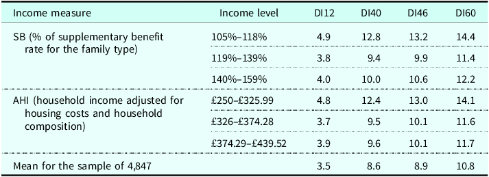
Table 3 presents mean deprivation scores for income categories based on the main cut-off points established in this stage of the analysis. Additionally, it includes the 140–159 per cent SB income range used by Townsend for his mode calculations, and an AHI income range that covers the same proportion of its income distribution (£374.29–£439.52). Table 3 shows that mean DI scores are stable across the higher income categories before leaping upwards below the noted income cut-off points. In view of Townsend’s claim that deprivation among these respondents rocketed below 140 per cent of SB, it is remarkable that mean deprivation scores in Table 3 are all significantly (P < 0.05) lower in the middle SB income category (119–139 per cent) than in the higher one (140–159 per cent)Footnote 6 . For AHI, the corresponding deprivation scores’ differences are all nonsignificant.
Average (mean) deprivation scores at various income levels

Table 3 Long description
A table comparing deprivation scores at various income levels. The table has 3 rows and 5 columns. The columns are labeled Income measure, Income level, DI12, DI40, DI46, and DI60. The rows are labeled with different income measures and levels, and the values represent the mean deprivation scores. Row 1: SB (percent of supplementary benefit rate for the family type), 105 percent-118 percent, 4.9, 12.8, 13.2, 14.4. Row 2: SB, 119 percent-139 percent, 3.8, 9.4, 9.9, 11.4. Row 3: SB, 140 percent-159 percent, 4.0, 10.0, 10.6, 12.2. Row 4: AHI (household income adjusted for housing costs and household composition), 250 GBP-325.99 GBP, 4.8, 12.4, 13.0, 14.1. Row 5: AHI, 326 GBP-374.28 GBP, 3.7, 9.5, 10.1, 11.6. Row 6: AHI, 374.29 GBP-439.52 GBP, 3.9, 9.6, 10.1, 11.7. Row 7: Mean for the sample of 4,847, 3.5, 8.6, 8.9, 10.8.
Source: Poverty in the United Kingdom data, 1968–69; n (numbers in each category) are SB:105%–118% = 301, 119%–139% = 597, 140–159% = 563; AHI: £250–£325.99 = 569, £326–374.28 = 412, £374.29–£439.52 = 554.
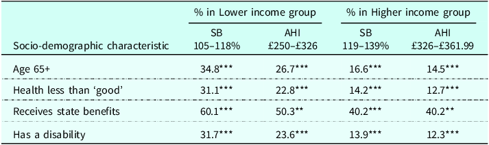
Some of the jump in deprivation at around 119 per cent (SB) and £326/£316 (AHI) might be accounted for by socio-demographic groups that suffer relatively high deprivation levels being overrepresented in the lower income groups; all four social categories available in the dataset that this applied to feature in Table 4.
Socio-demographic groups’ membership of income groups within the ranges of 105–139% of SB rates and £250–£361.99 of AHI

Table 4 Long description
The table presents socio-demographic characteristics and their percentages within lower and higher income groups, divided by specific income ranges for Standard Budget (SB) and Actual Household Income (AHI). The table has 4 rows and 5 columns. Column headers are: Socio-demographic characteristic, % in Lower income group SB 105-118%, % in Lower income group AHI 250-326, % in Higher income group SB 119-139%, % in Higher income group AHI 326-361.99. Row 1: Age 65+, 34.8***, 26.7***, 16.6***, 14.5***. Row 2: Health less than 'good', 31.1***, 22.8***, 14.2***, 12.7***. Row 3: Receives state benefits, 60.1***, 50.3**, 40.2***, 40.2**. Row 4: Has a disability, 31.7***, 23.6***, 13.9***, 12.3***. The table highlights notable trends and comparisons across different socio-demographic characteristics and income groups.
Source: Poverty in the United Kingdom data, 1968/69; n = 845 (AHI tests), n = 967 (SB tests); ** = <0.01, *** = <0.001; significance levels are for differences in socio-demographic group’ membership of different income categories.
In Table 4, socio-demographic categories are ‘cut’ at points that maximise the strength of their correlation with deprivation; for example, those age ‘65 and over’ are included, rather than those of at least state pension age (which was 60 for UK women and 65 for men in 1968/69), as the former has a stronger correlation. Two of the socio-demographic categories – those with poor/fair health and the disabled – are also deprivation indicators (numbers 41 and 43, see Appendix). If those in at least three of the four categories in Table 4 are removed from the analysis, this reduces correlation strengths only marginally for the AHI income measure; for example, for DI40 the Cohen’s ‘d’ score falls only from −0.68 to −0.63. For SB the effect is slightly greater, reducing the strength of DI40’s negative correlation with it from −0.72 to −0.57. Furthermore, logistic regression analysis that included DI variables alongside combinations of the four variables in Table 4 as predictors of membership of the lower income group virtually never found that any of the four variables were significant predictors. The exception was ‘Age 65+’, which occasionally delivered significant though very weak odds ratios, all below 1.5, while DI predictors often delivered odds ratios of more than three. Thus, much of the notable jump in deprivation scores below 119 per cent of SB rates and £326 AHI remains a mystery.
Conclusion
The influence of Peter Townsend’s 1968/69 poverty survey can be seen in poverty research today, but his claim that analyses of its data established a scientifically meaningful poverty ‘threshold’, below which deprivation increased at a faster rate in relation to income, was controversial. The new analysis presented here found no threshold, even when Townsend’s research decisions were replicated. Instead, the findings supported specific points made by two of Townsend’s fiercest critics. Mansfield (Reference Mansfield1986) claimed that Townsend chose a ‘mode’ over a ‘mean’ deprivation measure to boost his claim that a threshold existed at his preferred income level of 140 per cent of SB rates; here it was shown that mean deprivation even decreased significantly immediately below 140 per cent. Piachaud’s (Reference Piachaud1987) assertion, that Desai’s (Reference Desai and Golding1986) mean-based analysis of Townsend’s data could have found a more marked difference in deprivation rates at a lower income level than his (Desai’s) 150 per cent of SB ‘threshold’, was also supported; the strongest correlation was established with the data split at 119 per cent.
By showing that even Townsend’s much-trumpeted income threshold was arbitrary, and by highlighting the widely repeated empirical finding that income is not a good indicator of actual deprivation, this article provides a timely reminder of the serious limitations of income-based poverty lines such as the current UK government’s main ‘60 per cent of median income’ measure. As Edmiston (Reference Edmiston2022) argued, the application of a range of other poverty measures alongside that conventional 60 per cent yardstick, accompanied by reflection on each measure’s implications, strengths and limitations, will improve debates about poverty measurement and, consequentially, aid the design and evaluation of a range of anti-poverty policies. Indeed, the rigid use of the 60 per cent line to repeatedly identify similar groups of people as ‘poor’ and ‘non-poor’ risks limiting our understanding of the relationship between poverty and other social science phenomena, such as crime rates and educational attainment levels.
Given the unattainability of a meaningful poverty ‘threshold’ produced by detached scientific observation, the consensual deprivation method arguably offers the most meaningful poverty measure available, due to its advantage of being embedded in the feelings and experiences of those studied. The UK government’s augmentation of its main income-based measure with a consensual deprivation one can therefore be viewed positively. Alongside the percentage of children deemed to be in ‘deep material poverty’ due to lacking an arbitrary ‘four or more’ publicly endorsed essentials, hopefully the percentage lacking at least two, three and five will be widely noticed too.
Acknowledgements
I thank Suzanne McMorrow at Queen’s University, Belfast, for her advice about graphs, and the anonymous reviewers for their helpful comments.
Competing interests
I confirm that there is no conflict of interest.
APPENDIX: Townsend’s (Reference Townsend1979, 1173-1176) 60 ‘deprivation Indicators’ (*=included in Townsend’s 12-item sub-index [DI12])
Dietary
-
1. At least one day without cooked meal in last two weeks*
-
2. No fresh meat most days of week*
-
3. School child does not have school meals
-
4. Has not had cooked breakfast most days of the week*
-
5. Household does not have a Sunday joint three weeks in four*
-
6. Fewer than three pints of milk per person per week
Clothing
-
7. Inadequate footwear for both wet and fine weather
-
8. Income unit buys second-hand clothes often or sometimes
-
9. Income unit misses clothing club payments often or sometimes
-
10. (Married women) No new winter coat in last three years
Fuel and light
-
11. No electricity or light only (not power)
-
12. Short of fuel sometimes or often
-
13. No central heating
-
14. No rooms heated (or only one)
Household
-
15. No TV facilities
-
16. No refrigerator*
-
17. No telephone
-
18. No record player
-
19. No radio
-
20. No washing machine
-
21. No vacuum cleaner
-
22. No carpet
-
23. No armchair
Housing
-
24. No sole use of four amenities conditions (indoor WC, sink or washbasin, bath or shower, and cooker)*
-
25. Structural defects
-
26. Structural defects believed dangerous to health
-
27. Overcrowded (in terms of number of bedrooms)
Conditions at work (severity, security, amenities and welfare benefits)
-
28. Works mainly or entirely outdoors
-
29. Stands or walks at work all the time
-
30. Working fifty or more hours last week
-
31. At work before 8 a.m. or working at night
-
32. Poor outdoor amenities of work
-
33. Poor indoor amenities of work
-
34. Unemployed for two weeks or more during previous twelve months
-
35. Subject to one week’s entitlement to notice or less
-
36. No wages or salary during sickness
-
37. Paid holidays of two weeks or less
-
38. No meals paid or subsidised by employer
-
39. No entitlement to occupational pension
Health
-
40. Health poor or fair
-
41. Sick from work five or more weeks last year
-
42. Ill in bed fourteen days or more last year
-
43. Has disability condition
-
44. Has some or severe disability
Educational
-
45. Fewer than ten years’ education
Environmental
-
46. No garden or yard, or shared
-
47. If garden, too small to sit in
-
48. Air dirty or foul-smelling
-
49. No safe place for child (1-4) to play
-
50. No safe place for child (5-10) to play
Family
-
51. Difficulties indoors for child to play
-
52. Child not had friend in to play in last four weeks*
-
53. Child not had party last birthday*
-
54. Household spent less than additional £10 last Christmas
Recreational
-
55. No afternoons or evenings out in last two weeks*
-
56. No holiday in last twelve months away from home*
Social
-
57. No emergency help available, e.g. illness
-
58. No one coming to meal or snack in last four weeks*
-
59. Not been out to meal or snack with relatives or friends in last four weeks*
-
60. Moved house at least twice in last two years