1 Introduction
For onshore wind farms, unlike the offshore ones, there is a high chance that they are located on a non-flat complex terrain, where wind resource potential is high. This chance keeps increasing with the current expansion of wind power capacity. On the other hand, most of the studies on wind turbine wakes have been carried out assuming a flat underlying terrain, and relatively little attention has been devoted to wakes over topography. Therefore, more careful and refined investigation of wind turbine wakes over topography is much needed and it can highly contribute to better wind-farm site selections and configuration designs.
Although the problem of wakes on topography has received little attention, there is a rich literature on the subject of atmospheric boundary-layer flows over topography. There are numerous experimental, numerical and analytical investigations on this subject, for a review of which Belcher & Hunt (Reference Belcher and Hunt1998) and Wood (Reference Wood2000) can be consulted. Before addressing the issue of wind turbine wakes over topography, we cast a brief retrospective look at the key analytical developments of flow over hills (without the presence of turbines), as they play a significant role in the contents of the present paper. A similar kind of review but for experimental and numerical studies is also available in Shamsoddin & Porté-Agel (Reference Shamsoddin and Porté-Agel2017a ) (e.g. studies such as Britter, Hunt & Richards Reference Britter, Hunt and Richards1981; Baskaran, Smits & Joubert Reference Baskaran, Smits and Joubert1987; Taylor & Teunissen Reference Taylor and Teunissen1987; Gong, Taylor & Dörnbrack Reference Gong, Taylor and Dörnbrack1996; Ishihara, Hibi & Oikawa Reference Ishihara, Hibi and Oikawa1999; Iizuka & Kondo Reference Iizuka and Kondo2004; García-Villalba et al. Reference García-Villalba, Li, Rodi and Leschziner2009; Berg et al. Reference Berg, Mann, Bechmann, Courtney and Jørgensen2011; Diebold et al. Reference Diebold, Higgins, Fang, Bechmann and Parlange2013; Giometto et al. Reference Giometto, Katul, Fang and Parlange2017; Razavi & Sarkar Reference Razavi and Sarkar2018). Subsequently, the interaction of wind turbines and topography is presented in the following subsection.
1.1 Analytical studies of flow over hills
From the 1940s to the 1980s, substantial effort and significant progress was made in the theoretical study and characterization of different features of the flow over topography. This nearly half a century of extensive investigation can be essentially divided into two periods (Wood Reference Wood2000); in the first period, which extends from the 1940s to the 1960s, most of the theoretical work was focused on the inviscid response of stably stratified flows to hills (for detailed reviews about the research in this period see Corby (Reference Corby1954), Wurtele, Sharman & Datta (Reference Wurtele, Sharman and Datta1996), among others).
The second period commenced with the groundbreaking analysis of Jackson & Hunt (Reference Jackson and Hunt1975) who developed a linear solution for two-dimensional turbulent flows over low hills with arbitrary shapes. After using perturbation methods and performing an order of magnitude analysis on the Navier–Stokes equations (continuity and two equations of motion in the horizontal and vertical directions), they argued that the flow can be considered to be divided into two layers: a thin inner layer in which the perturbation turbulent shear stresses are significant and modelled by a simple mixing-length model; and an outer layer in which the perturbation stresses are shown to be negligible and the disturbance to be almost irrotational. By asymptotic expansion of the perturbation variables (pressure and two components of velocity), the linearized, Fourier-transformed equations were solved, and analytical solutions (to the leading order) were obtained in wavenumber space.
The paper of Jackson and Hunt influenced and inspired numerous researchers in the forthcoming years. Mason & Sykes (Reference Mason and Sykes1979) extended the model to three dimensions and compared the results with their field data. Next, Sykes (Reference Sykes1980) presented his own asymptotic analysis of a turbulent boundary-layer flow encountering a small two-dimensional hump. While his analysis was, in many ways, similar to that of Jackson and Hunt, it had major distinctions and contributions. First, instead of two layers, he considered three layers by adding a very thin wall layer to impose the surface boundary condition more consistently. He also used a second-order closure model to model the Reynolds stress perturbations and was able to calculate the net force perturbation (pressure drag) on the obstacle. Further modifications to the linear theory were introduced by Hunt, Leibovich & Richards (Reference Hunt, Leibovich and Richards1988), who developed an analysis for turbulent shear flows over two- and three-dimensional hills, which is capable of dealing with different upwind velocity profiles. By keeping the wall layer, which was proposed by Sykes (Reference Sykes1980), and subdividing the inviscid outer layer of Jackson and Hunt theory into two sublayers, they considered a total of four different layers in their analysis. In this new description, the middle layer was newly introduced to allow for significant shear in the upstream flow. Other advancements of the theory were achieved by Taylor, Walmsley & Salmon (Reference Taylor, Walmsley and Salmon1983) who employed a wavenumber-dependent strategy to assign a specific horizontal length scale to each wavenumber in Fourier space. In the 1990s, attempts to analytically include nonlinear effects in the solution of the flow over low-slope hills are found in the works of Xu & Taylor (Reference Xu and Taylor1992) and Xu, Ayotte & Taylor (Reference Xu, Ayotte and Taylor1994). They included the nonlinear terms as source terms in the governing equations, and then calculated the solution iteratively in spectral space, while keeping the nonlinear terms in physical space.
1.2 Wind turbines and topography
Experimental (both wind tunnel and field) measurements of wind turbine wakes over hilly terrain started in the early 1990s (e.g. Taylor & Smith Reference Taylor, Smith, Quarton and Fenton1991; Stefanatos et al. Reference Stefanatos, Voutsinas, Rados, Zervos and Tsipouridis1994; Helmis et al. Reference Helmis, Papadopoulos, Asimakopoulos, Papageorgas and Soilemes1995; Stefanatos, Morfiadakis & Glinou Reference Stefanatos, Morfiadakis, Glinou, Zervos, Ehmann and Helm1996). More recently, various cases of wind turbine siting on topography have been studied. Tian et al. (Reference Tian, Ozbay, Yuan, Sarkar and Hu2013) considered an array of five turbines distributed on a single hill, and compared the wind-farm performance with the flat-terrain case. Yang et al. (Reference Yang, Howard, Guala and Sotiropoulos2015), on the other hand, placed a turbine downstream of a single hill, and observed that the turbine wake recovery rate increases due to the turbulence generated by the hill. Moreover, Hyvärinen & Segalini (Reference Hyvärinen and Segalini2017a ) performed measurements of the flow around two tandem wind turbines which were sited on a terrain consisting of a series of sinusoidal hills. They also observed a faster wake recovery, and, as they mentioned, ‘a positive impact on the wind-turbine performance’ due to the presence of the hills.
Furthermore, numerical models have also been developed for this problem (e.g. Voutsinas, Rados & Zervos Reference Voutsinas, Rados, Zervos and Palz1990; Hemon, Huberson & Zervos Reference Hemon, Huberson, Zervos, Quarton and Fenton1991; Günther, Fallen & Wolfanger Reference Günther, Fallen, Wolfanger, Garrad, Palz and Scheller1993; Ansorge et al. Reference Ansorge, Fallen, Günther, Ruh, Wolfanger and Tsipouridis1994; Chaviaropoulos & Douvikas Reference Chaviaropoulos, Douvikas, Petersen, Jensen, Rave, Helm and Ehmann1999; Ivanova & Nadyozhina Reference Ivanova and Nadyozhina2000; Migoya et al. Reference Migoya, Crespo, García, Moreno, Manuel and Costa2007). More recently, Politis et al. (Reference Politis, Prospathopoulos, Cabezon, Hansen, Chaviaropoulos and Barthelmie2012) performed RANS (Reynolds-averaged Navier–Stokes) simulations of both a real wind farm on a complex terrain and a single turbine sited on top of a single hill. They have observed that the wake recovery is slower with respect to the flat-terrain case. Moreover, using terrain-following coordinates, Shamsoddin & Porté-Agel (Reference Shamsoddin and Porté-Agel2017a ) performed large-eddy simulation (LES) of flow through a wind farm sited on a single hill and validated the results using the dataset of Tian et al. (Reference Tian, Ozbay, Yuan, Sarkar and Hu2013). Employing a different approach, Segalini (Reference Segalini2017) used the linearized continuity and momentum equations to solve for the flow field around turbines located on low-slope topography. This method has the advantage of incurring significantly less computational cost. In addition to these, there have also been other numerical studies on this subject both for real complex terrains (e.g. Schulz et al. Reference Schulz, Klein, Weihing, Lutz and Krämer2014; Yang et al. Reference Yang, Sotiropoulos, Conzemius, Wachtler and Strong2014; Castellani et al. Reference Castellani, Astolfi, Burlando and Terzi2015, Reference Castellani, Astolfi, Mana, Piccioni, Becchetti and Terzi2017; Berg et al. Reference Berg, Troldborg, Sørensen, Patton and Sullivan2017) and idealized hills (e.g. Yang et al. Reference Yang, Howard, Guala and Sotiropoulos2015; Zheng et al. Reference Zheng, Tian, Qin and Hu2017).
The common simple method used in industry to model the effect of topography on turbine wakes is the idea of superposition, in which the turbine velocity deficit over flat terrain is superposed on the flow over the topography (without the turbines). This method has been used by several researchers (e.g. Crespo & Hernández Reference Crespo, Hernández, Palz and Sesto1986; Crespo et al. Reference Crespo, Manuel, Grau, Hernández, Garrad, Palz and Scheller1993; Hyvärinen & Segalini Reference Hyvärinen and Segalini2017b ) and in some cases (e.g. Crespo et al. Reference Crespo, Manuel, Grau, Hernández, Garrad, Palz and Scheller1993; Hyvärinen & Segalini Reference Hyvärinen and Segalini2017b ) has resulted in acceptable results. However, its general applicability, even for hills of moderate slope, has been called into question (Politis et al. Reference Politis, Prospathopoulos, Cabezon, Hansen, Chaviaropoulos and Barthelmie2012; Segalini Reference Segalini2017).
In this paper, we aim to investigate how a single hill affects the wake of a wind turbine sited upstream of it. We are going to answer questions such as: why have Politis et al. (Reference Politis, Prospathopoulos, Cabezon, Hansen, Chaviaropoulos and Barthelmie2012) observed a slower wake recovery when the turbine is located on the hilltop (compared with flat-terrain case), whereas others (Yang et al. Reference Yang, Howard, Guala and Sotiropoulos2015; Hyvärinen & Segalini Reference Hyvärinen and Segalini2017a ) have mostly reported a faster wake recovery on hilly terrain? We will see that the reasons for each of these two trends have completely different natures. We also present an analytical modelling framework which enables us to predict how a hill affects a turbine wake flow. In doing so, we use the substantial and valuable analytical developments of flow over hills (e.g. Hunt et al. Reference Hunt, Leibovich and Richards1988), and we also take advantage of some wake-specific studies of the pressure-gradient effect on wake flows (e.g. Liu, Thomas & Nelson Reference Liu, Thomas and Nelson2002; Shamsoddin & Porté-Agel Reference Shamsoddin and Porté-Agel2017b , Reference Shamsoddin and Porté-Agel2018). Moreover, we perform LES of such flows in order to test our model and also to acquire more detailed insight into these flows.
This article is structured in the following manner. In § 2, the analytical framework is derived and illustrated. The LES set-up and some key LES qualitative results are described in § 3. Special attention is paid to the wake on the leeward side of the hill in § 4. At this stage, we will be ready to test the developed analytical framework against LES data in § 5. In § 6, the effect of the pressure gradient on wake recovery is inspected more thoroughly, and finally § 7 concludes the paper.
2 An analytical modelling framework for wake flows over hills
2.1 Problem formulation
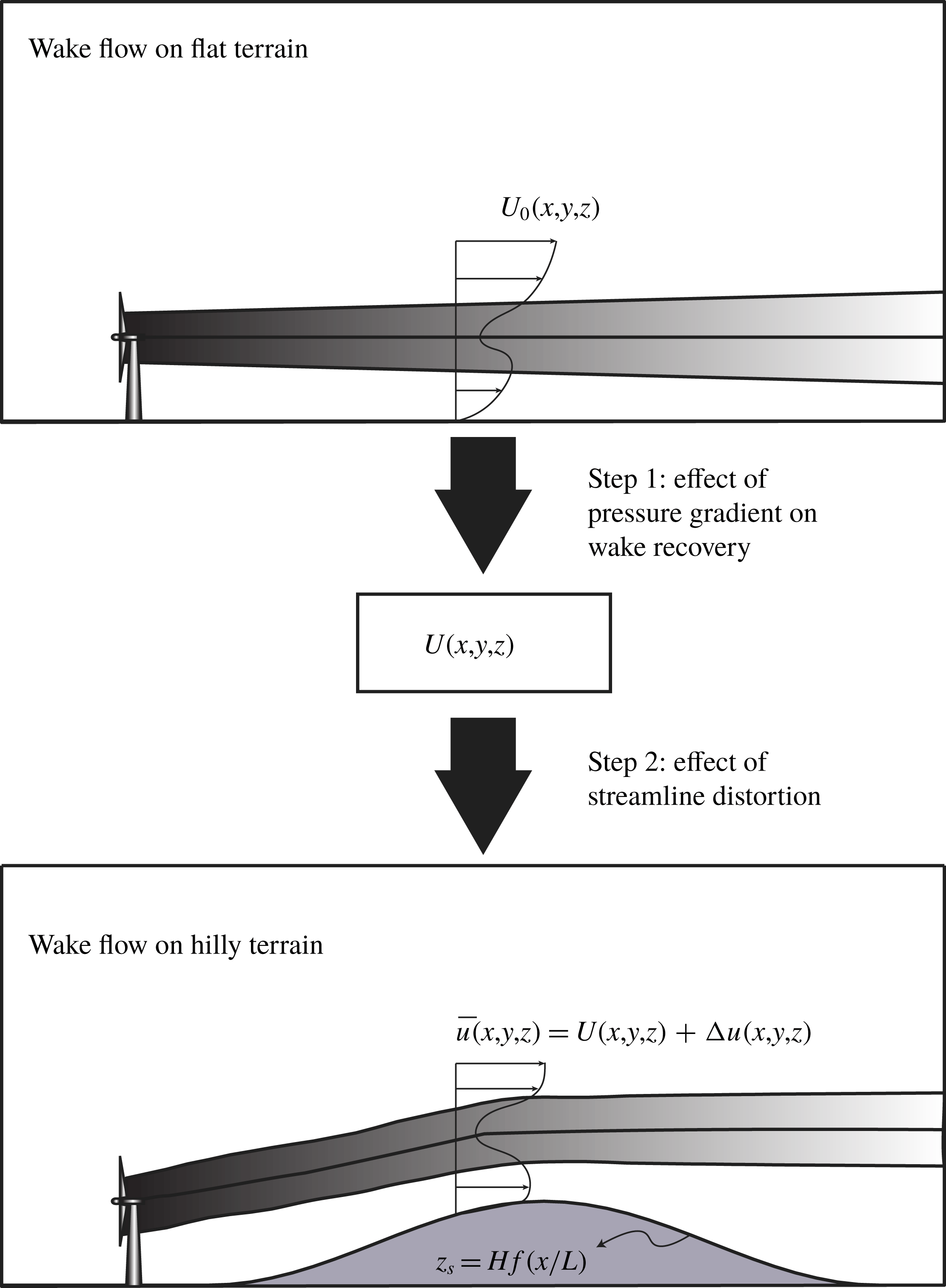
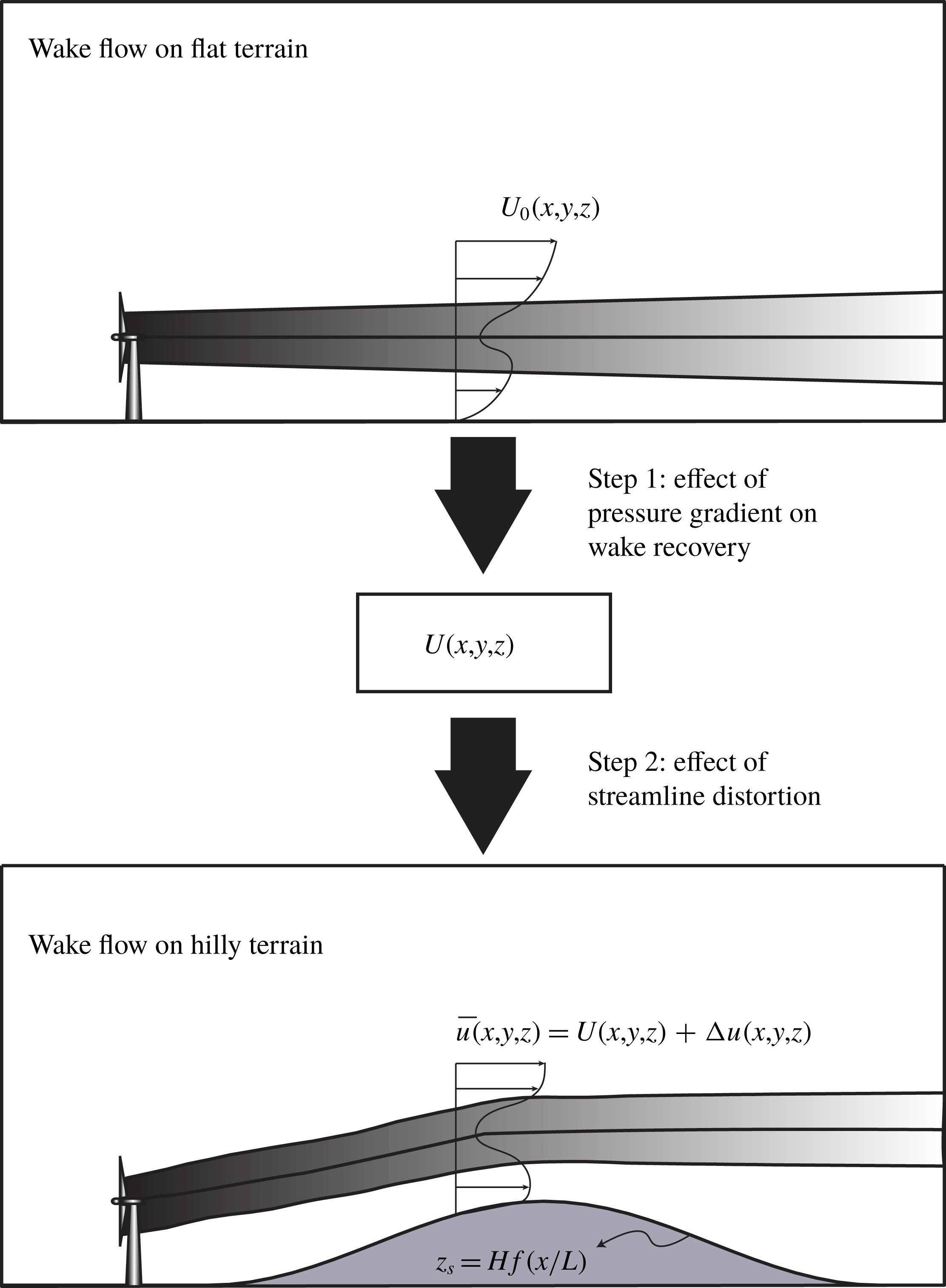
The objective of this section is to develop an analytical model which enables us to predict the evolution of a turbine wake flow over a two-dimensional (2-D) hill of moderate slope. More specifically, we are interested in solving the following problem: for a given wake over a flat terrain, how does the introduction of a 2-D hill downwind of the turbine perturb the wake flow field? In particular, we are interested in the wake recovery rate, the mean velocity and velocity deficit profiles and the wake trajectory in the presence of the hill. The starting and end points of the problem are shown in the schematic of figure 1.
In general, the topography is considered to produce two major effects on the flow passing above it: (i) the non-zero pressure gradient up- and downwind of the hilltop, and (ii) curvature of the streamline (for instance, see Nakayama Reference Nakayama1987; Baskaran, Smits & Joubert Reference Baskaran, Smits and Joubert1991). The pressure-gradient effect is especially important for wake flows above hills, because it considerably affects the wake recovery, i.e. depending on the sign of the pressure gradient, the wake recovers faster or slower with respect to a wake in zero pressure gradient. In our approach to modelling a wake flow over a hill we decouple the analysis of these two effects on the wake. In accordance with these two major effects, the modelling framework that we will present comprises two steps. In the first step, we predict how the induced pressure gradient by the hill alters the wake recovery evolution. In the second step, we calculate how the wake (which is now already modified by the effect of the pressure gradient) flows over the hill by taking into account the distortion of the streamlines caused by the hill. In doing so, we model these two effects separately. This two-step approach is also shown in figure 1. Each of these two steps will be described in the next two subsections (§§ 2.2 and 2.3).
Schematic of the problem and the modelling framework.
2.2 Effect of the hill-induced pressure gradient on the wake recovery
It is known that hills produce non-zero pressure gradients in the flow above them. Particularly, hills induce mainly a favourable pressure gradient (FPG) on their windward side and an adverse pressure gradient (APG) on their leeward side (normally a slight APG precedes the FPG on the windward side, but its magnitude is much smaller). This is equivalent to the fact that the flow mainly undergoes an acceleration upwind of the hilltop and a deceleration downwind of it. On the other hand, the pressure gradient affects the wake recovery characteristics. The wake centre velocity recovers faster in FPG conditions and slower in APG conditions (with respect to the zero-pressure-gradient (ZPG) case). The wake width, however, grows more rapidly under APG and more slowly under FPG compared with the ZPG case. These trends have been shown for planar wakes in the works of Rogers (Reference Rogers2002) (numerically), Liu et al. (Reference Liu, Thomas and Nelson2002) and Thomas & Liu (Reference Thomas and Liu2004) (experimentally) and recently in Shamsoddin & Porté-Agel (Reference Shamsoddin and Porté-Agel2017b ) (analytically). Moreover, Shamsoddin & Porté-Agel (Reference Shamsoddin and Porté-Agel2018) have recently shown that the above trends also apply to axisymmetric wakes (which is the case for a wind turbine wake) by using both an analytical approach and LES data.
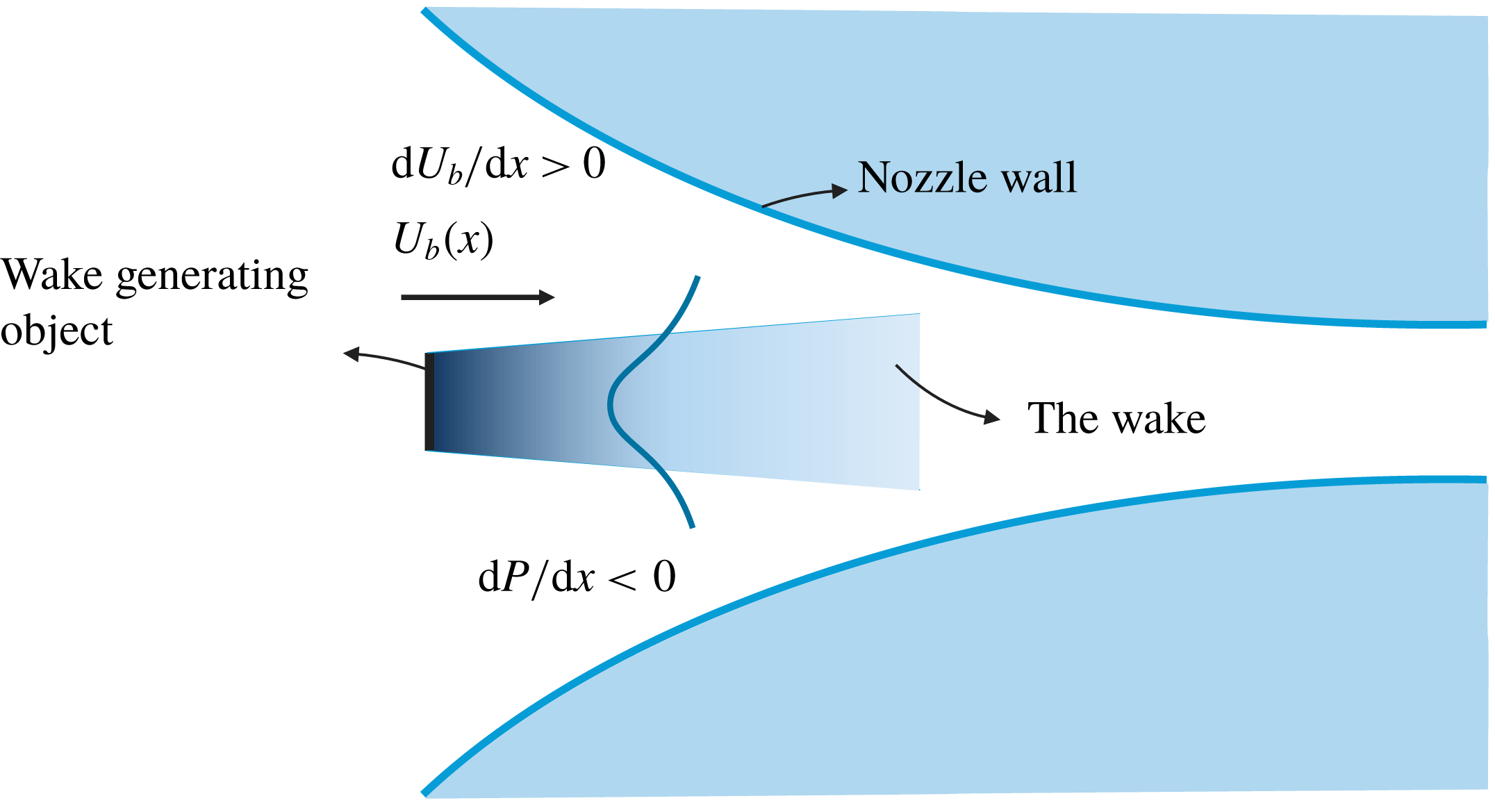
Schematic of a wake under a favourable pressure gradient, as an example.

Figure 2 shows a simple schematic of a wake under a pressure gradient; in this figure, a wake in FPG is shown as an example. Herein, we use the model developed by Shamsoddin & Porté-Agel (Reference Shamsoddin and Porté-Agel2018) to model the effect of the hill-induced pressure gradient on the axisymmetric wake of a wind turbine. The model needs two inputs. First, the mean velocity evolution in the absence of the turbine which is indicative of the imposed pressure gradient. Second, the wake width of the corresponding ZPG case, which, in this case, would be the wake over a flat terrain.
The mean velocity deficit profiles of a turbulent axisymmetric wake are taken to have a self-similar Gaussian shape:
 $$\begin{eqnarray}{\displaystyle \frac{U_{b}(x)-\overline{u}(x,r)}{U_{b}(x)}}\equiv C(x)\text{e}^{-(r^{2}/2\unicode[STIX]{x1D6FF}^{2})},\end{eqnarray}$$
where
 $x$
is the streamwise direction,
 $r$
is the radial direction from the wake centre,
 $\overline{u}(x,r)$
is the velocity (hereafter, by velocity, we imply the mean streamwise velocity, unless otherwise stated) of the wake flow,
 $U_{b}(x)$
is the velocity of the flow under a pressure gradient but without the wake,
 $C(x)$
is a function determining the maximum velocity deficit at each
 $x$
-position and
 $\unicode[STIX]{x1D6FF}(x)$
is the wake width. As mentioned earlier,
 $U_{b}(x)$
is the velocity of the flow in the absence of the wake which is affected by the imposed pressure gradient. For example, in the schematic of figure 2,
 $U_{b}(x)$
indicates an accelerating flow. Now, the question is: what is
 $U_{b}(x)$
for the case of wake flow over a hill? Of course, in this case, the velocity of the flow is not uniform and it changes with height; however, we can (as an approximation) consider
 $U_{b}(x)$
to be equal to the velocity at a distance equal to the hub height (
 $Z_{h}$
) from the ground in the case without the wind turbine, i.e.
 $U_{nw}^{h}(x)$
(for a more detailed discussion on
 $U_{nw}^{h}(x)$
, see appendix A).
For
 $C(x)$
, the following ordinary differential equation (ODE) can be obtained (see Shamsoddin & Porté-Agel Reference Shamsoddin and Porté-Agel2018):
 $$\begin{eqnarray}{\displaystyle \frac{\text{d}C(x)}{\text{d}x}}={\displaystyle \frac{-1}{\left({\displaystyle \frac{U_{b}^{4}}{\unicode[STIX]{x1D706}_{0}^{2}}}\right)\left(3C^{2}-2C^{3}\right)}}\left[{\displaystyle \frac{1}{4}}{\displaystyle \frac{\text{d}U_{b}^{4}}{\text{d}x}}{\displaystyle \frac{C^{3}}{\unicode[STIX]{x1D706}_{0}^{2}}}+\left(C^{3}-{\displaystyle \frac{C^{4}}{2}}\right){\displaystyle \frac{\text{d}}{\text{d}x}}\left({\displaystyle \frac{U_{b}^{4}}{\unicode[STIX]{x1D706}_{0}^{2}}}\right)\right],\end{eqnarray}$$
with the boundary condition
 $$\begin{eqnarray}C(x_{i})=C_{0}(x_{i}),\end{eqnarray}$$
where
 $C_{0}(x)$
and
 $\unicode[STIX]{x1D706}_{0}(x)$
are
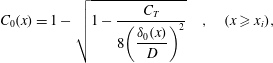 $$\begin{eqnarray}C_{0}(x)=1-\sqrt{1-{\displaystyle \frac{C_{T}}{8\left({\displaystyle \frac{\unicode[STIX]{x1D6FF}_{0}(x)}{D}}\right)^{2}}}}\quad ,\quad (x\geqslant x_{i}),\end{eqnarray}$$
and
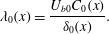 $$\begin{eqnarray}\unicode[STIX]{x1D706}_{0}(x)={\displaystyle \frac{U_{b0}C_{0}(x)}{\unicode[STIX]{x1D6FF}_{0}(x)}}.\end{eqnarray}$$
In these equations, the subscript
 $0$
indicates a quantity in the ZPG case,
 $D$
is the diameter of the wake-generating object and
 $C_{T}$
is the thrust coefficient of the turbine. The condition
 $(x\geqslant x_{i})$
is only to make sure that the expression under the square root always remains non-negative. Finally,
 $\unicode[STIX]{x1D6FF}$
can be expressed as
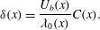 $$\begin{eqnarray}\unicode[STIX]{x1D6FF}(x)={\displaystyle \frac{U_{b}(x)}{\unicode[STIX]{x1D706}_{0}(x)}}C(x).\end{eqnarray}$$
It can be shown that the following asymptotic solution (designated as
 $\widetilde{C}(x)$
) for the ODE of (2.2) can be obtained for sufficiently large
 $x$
(Shamsoddin & Porté-Agel Reference Shamsoddin and Porté-Agel2018):
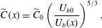 $$\begin{eqnarray}\widetilde{C}(x)=\widetilde{C}_{0}\left({\displaystyle \frac{U_{b0}}{U_{b}(x)}}\right)^{5/3},\end{eqnarray}$$
where
 $\widetilde{C}_{0}=D^{2}C_{T}/(16\unicode[STIX]{x1D6FF}_{0}^{2})$
is the asymptotic ZPG solution for
 $\widetilde{C}_{0}$
, which is equal to the second-order Taylor expansion of the full solution of
 $C_{0}(x)$
, i.e. (2.4), in terms of
 $\unicode[STIX]{x1D6FF}_{0}^{-1}$
.
The velocity
 $U_{nw}^{h}$
(which is used to replace
 $U_{b}(x)$
in the above equations) can be obtained by linearized models such as the one proposed by Jackson & Hunt (Reference Jackson and Hunt1975). We will elaborate more on this in the next subsection and also in appendix A. Up to this stage, with (2.2) and (2.6), one can obtain the wake evolution under the pressure gradient caused by the hill.
2.3 Effect of the hill-induced streamline distortion
In this subsection, we employ a linearized perturbation approach to calculate how the wake moves over the hill. One important assumption of this method is that the flow remains attached to the hill, and there is no flow separation. For a hill of moderate slope, this assumption holds for the windward side of the hill. For the leeward side, however, this assumption normally no longer remains valid. Even if we do not have a flow separation (with the strict definition of having negative velocities at certain locations), we usually have the so-called ‘non-separated sheltering’ on the leeward side of the hill (Belcher, Newley & Hunt Reference Belcher, Newley and Hunt1993; Belcher & Hunt Reference Belcher and Hunt1998; Belcher Reference Belcher1999). It is also already known that linearized perturbation models (without turbines) do not result in sufficiently accurate predictions on the leeward side of the hills (even with moderate slopes) due to this non-separated sheltering effect (e.g. Britter et al. Reference Britter, Hunt and Richards1981). For the leeward side of the hill, a special treatment will be used, which will be presented in § 4.
Herein, we use a linearized perturbation approach, which is inspired by the work of Hunt et al. (Reference Hunt, Leibovich and Richards1988). In the present paper, we build on that model so that we can account for the evolution of the wind turbine wakes over hills. However, it should be noted that the fundamental difference of the present problem with the already available linearized models of boundary-layer flows over hills (e.g. Jackson & Hunt Reference Jackson and Hunt1975; Hunt et al.
Reference Hunt, Leibovich and Richards1988) is that in this case the base mean flow velocity (
 $U$
) is, in addition to
 $z$
, also a function of
 $x$
and
 $y$
. This will incur non-trivial differences in deriving the model, which we herein try to address. The hill considered here has a surface equation of
 $z_{s}=Hf(x/L)$
, where
 $H$
is the height at the hilltop,
 $L$
is the half-length of the hill,
 $f(x/L)\leqslant 1$
and
 $f(0)=1$
. In this analysis, we assume
 $H/L$
is sufficiently small. For example, for a typical hill of moderate slope
 $H/L\lesssim 0.3$
(Belcher & Hunt Reference Belcher and Hunt1998).
2.3.1 Governing equations and coordinate systems
The velocity components
 $\overline{u}$
,
 $\overline{v}$
and
 $\overline{w}$
are the mean streamwise, spanwise and vertical velocities in the case of the wake flow over a hill. This velocity field can be expressed in terms of the velocity field over a flat terrain (i.e. the base flow) and some perturbation velocities (see figure 1). The way that the perturbed velocities are linked to the base flow field depends on the coordinate system in which we express the flow. In general, there are two types of coordinates that can be envisaged for this purpose: Cartesian coordinates
 $(x,y,z)$
and terrain-following coordinates
 $(X,Y,Z)$
. The choice between these two types of coordinates in different regions of the flow should be based on the nature of the flow. The common practice is that as we move closer to the ground the terrain-following coordinates become more suitable, and at higher distances from the ground, Cartesian coordinates are preferred. In this section, we define the terrain-following coordinates as
 $X=x$
,
 $Y=y$
,
 $Z=z-Hf(x/L)$
. The perturbation velocities are defined in Cartesian and terrain-following coordinates by (2.8a
) and (2.9a
), respectively:
 $$\begin{eqnarray}\displaystyle \overline{u}(x,y,z) & = & \displaystyle U(x,y,z)+\unicode[STIX]{x0394}u(x,y,z),\end{eqnarray}$$
 $$\begin{eqnarray}\displaystyle \overline{v}(x,y,z) & = & \displaystyle \unicode[STIX]{x0394}v(x,y,z),\end{eqnarray}$$
 $$\begin{eqnarray}\displaystyle \overline{w}(x,y,z) & = & \displaystyle \unicode[STIX]{x0394}w(x,y,z),\end{eqnarray}$$
 $$\begin{eqnarray}\displaystyle \overline{p}(x,y,z) & = & \displaystyle P(x,y,z)+\unicode[STIX]{x0394}p(x,y,z),\end{eqnarray}$$
 $$\begin{eqnarray}\displaystyle \overline{u}_{t}(x,y,Z) & = & \displaystyle U(x,y,Z)+\unicode[STIX]{x0394}u_{t}(x,y,Z),\end{eqnarray}$$
 $$\begin{eqnarray}\displaystyle \overline{v}_{t}(x,y,Z) & = & \displaystyle \unicode[STIX]{x0394}v_{t}(x,y,Z),\end{eqnarray}$$
 $$\begin{eqnarray}\displaystyle \overline{w}_{t}(x,y,Z) & = & \displaystyle U{\displaystyle \frac{H}{L}}f^{\prime }\left({\displaystyle \frac{x}{L}}\right)+\unicode[STIX]{x0394}w_{t}(x,y,Z),\end{eqnarray}$$
 $$\begin{eqnarray}\displaystyle \overline{p}_{t}(x,y,Z) & = & \displaystyle P(x,y,Z)+\unicode[STIX]{x0394}p_{t}(x,y,Z),\end{eqnarray}$$
 $U$
is the mean streamwise velocity field over a flat terrain (i.e. the base flow), and the subscript
 $t$
indicates a quantity expressed in the terrain-following coordinates. The momentum and continuity equations for the flow are written as
 $$\begin{eqnarray}\displaystyle \overline{u}{\displaystyle \frac{\unicode[STIX]{x2202}\overline{u}}{\unicode[STIX]{x2202}x}}+\overline{v}{\displaystyle \frac{\unicode[STIX]{x2202}\overline{u}}{\unicode[STIX]{x2202}y}}+\overline{w}{\displaystyle \frac{\unicode[STIX]{x2202}\overline{u}}{\unicode[STIX]{x2202}z}} & = & \displaystyle -{\displaystyle \frac{1}{\unicode[STIX]{x1D70C}}}{\displaystyle \frac{\unicode[STIX]{x2202}\overline{p}}{\unicode[STIX]{x2202}x}}+{\displaystyle \frac{1}{\unicode[STIX]{x1D70C}}}{\displaystyle \frac{\unicode[STIX]{x2202}\unicode[STIX]{x1D70F}_{1j}}{\unicode[STIX]{x2202}x_{j}}},\end{eqnarray}$$
 $$\begin{eqnarray}\displaystyle \overline{u}{\displaystyle \frac{\unicode[STIX]{x2202}\overline{v}}{\unicode[STIX]{x2202}x}}+\overline{v}{\displaystyle \frac{\unicode[STIX]{x2202}\overline{v}}{\unicode[STIX]{x2202}y}}+\overline{w}{\displaystyle \frac{\unicode[STIX]{x2202}\overline{v}}{\unicode[STIX]{x2202}z}} & = & \displaystyle -{\displaystyle \frac{1}{\unicode[STIX]{x1D70C}}}{\displaystyle \frac{\unicode[STIX]{x2202}\overline{p}}{\unicode[STIX]{x2202}y}}+{\displaystyle \frac{1}{\unicode[STIX]{x1D70C}}}{\displaystyle \frac{\unicode[STIX]{x2202}\unicode[STIX]{x1D70F}_{2j}}{\unicode[STIX]{x2202}x_{j}}},\end{eqnarray}$$
 $$\begin{eqnarray}\displaystyle \overline{u}{\displaystyle \frac{\unicode[STIX]{x2202}\overline{w}}{\unicode[STIX]{x2202}x}}+\overline{v}{\displaystyle \frac{\unicode[STIX]{x2202}\overline{w}}{\unicode[STIX]{x2202}y}}+\overline{w}{\displaystyle \frac{\unicode[STIX]{x2202}\overline{w}}{\unicode[STIX]{x2202}z}} & = & \displaystyle -{\displaystyle \frac{1}{\unicode[STIX]{x1D70C}}}{\displaystyle \frac{\unicode[STIX]{x2202}\overline{p}}{\unicode[STIX]{x2202}z}}+{\displaystyle \frac{1}{\unicode[STIX]{x1D70C}}}{\displaystyle \frac{\unicode[STIX]{x2202}\unicode[STIX]{x1D70F}_{3j}}{\unicode[STIX]{x2202}x_{j}}},\end{eqnarray}$$
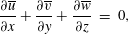 $$\begin{eqnarray}\displaystyle {\displaystyle \frac{\unicode[STIX]{x2202}\overline{u}}{\unicode[STIX]{x2202}x}}+{\displaystyle \frac{\unicode[STIX]{x2202}\overline{v}}{\unicode[STIX]{x2202}y}}+{\displaystyle \frac{\unicode[STIX]{x2202}\overline{w}}{\unicode[STIX]{x2202}z}} & = & \displaystyle 0,\end{eqnarray}$$
 $\unicode[STIX]{x1D70F}$
is the turbulent stress tensor.
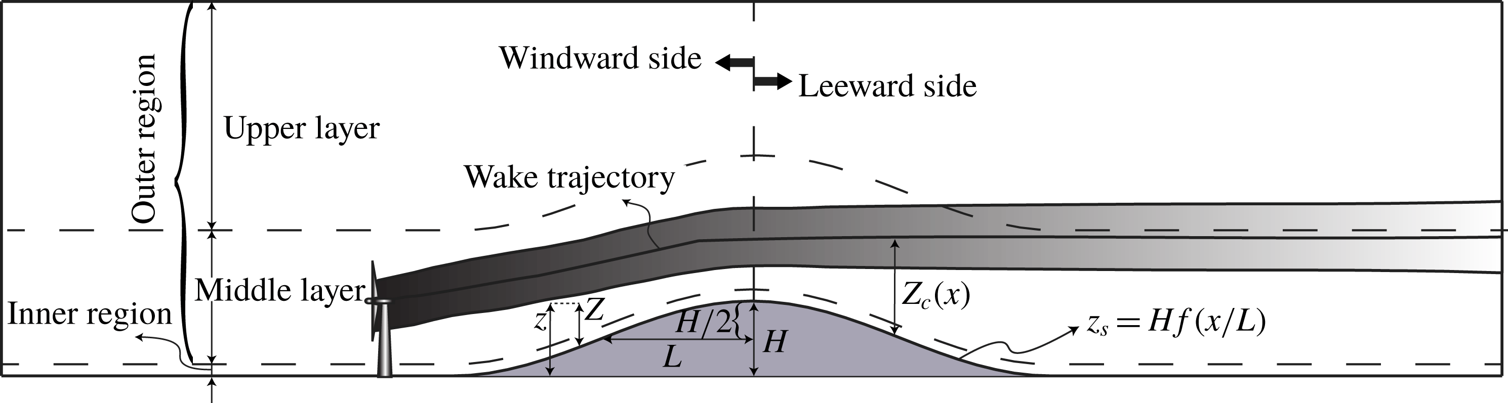
As shown in figure 3, flow over hills is commonly divided into two regions: (i) the inner region which is a relatively thin layer close to the ground, and (ii) the outer region which is located just above the inner region. The gradients of the perturbation turbulent stresses are considerable only in the inner region, and in the outer region they can be neglected (Jackson & Hunt Reference Jackson and Hunt1975). The turbine wake flows are essentially located in the outer region (for example see § 4.6 of Emeis Reference Emeis2013). It is also noteworthy that the inner region in a turbulent flow (unlike a laminar flow) has little effect on the outer region (Hunt et al.
Reference Hunt, Leibovich and Richards1988). That is why, in our analysis, we focus on the outer region. The thickness of the inner region
 $l$
can be determined by solving the equation
 $l\ln (l/z_{o})=2\unicode[STIX]{x1D705}^{2}L$
, where
 $\unicode[STIX]{x1D705}$
is the von Kármán constant and
 $z_{0}$
is the surface roughness length. Alternatively, one can use the following approximate explicit relation:
 $l=(1/8)z_{o}(L/z_{o})^{0.9}$
(Jackson & Hunt Reference Jackson and Hunt1975). For example, for a hill of 100 m height and
 $H/L=0.5$
on farmland (
 $z_{0}=0.1$
m), the height of the inner region would be approximately
 $l=11$
m.
Schematic of the second step of the model.
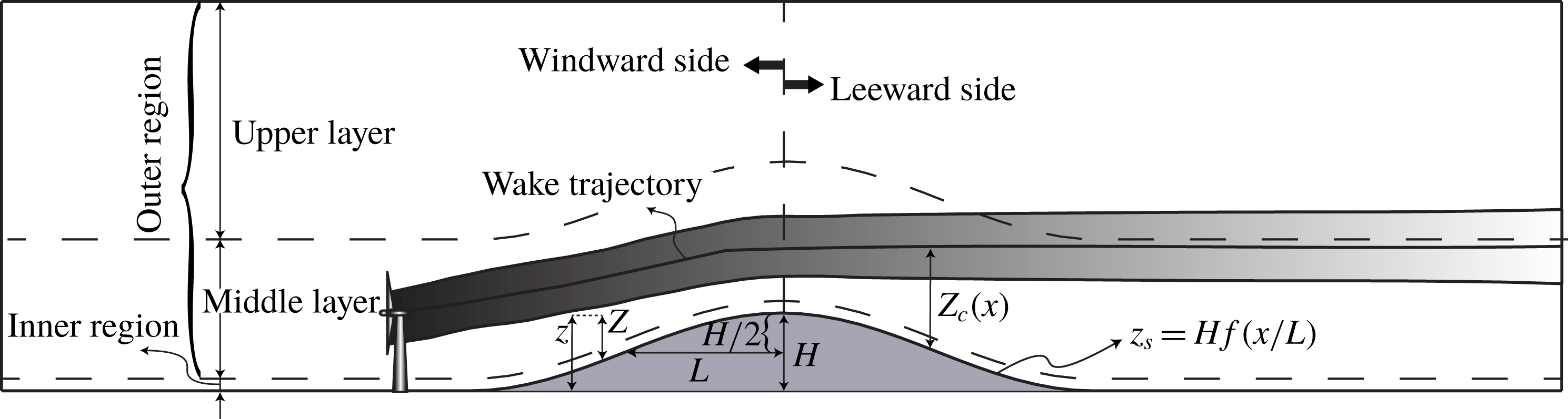
The outer region, in turn, is further divided into two layers: (i) the middle layer, and (ii) the upper layer. The main difference between these two layers, in this analysis, is in the type of coordinate system by which the perturbation velocities are related to the base flow. In the middle layer, the flow has a terrain-following nature (hence, we use the terrain-following coordinates (2.9a )), and in the upper layer, Cartesian coordinates have been proved to better capture the physics of the flow (Hunt et al. Reference Hunt, Leibovich and Richards1988). We continue this section by studying the flow in these two layers.
2.3.2 Upper layer
First, we consider the upper layer. Here, for the case of a 2-D hill, we can neglect the spanwise velocity
 $\overline{v}$
, and after linearization of the (2.10a
), we obtain the following equations for the perturbation velocities:
 $$\begin{eqnarray}\displaystyle U(x,y,z){\displaystyle \frac{\unicode[STIX]{x2202}\unicode[STIX]{x0394}u}{\unicode[STIX]{x2202}x}}+\unicode[STIX]{x0394}w{\displaystyle \frac{\unicode[STIX]{x2202}U(x,y,z)}{\unicode[STIX]{x2202}z}} & = & \displaystyle -{\displaystyle \frac{1}{\unicode[STIX]{x1D70C}}}{\displaystyle \frac{\unicode[STIX]{x2202}\unicode[STIX]{x0394}p}{\unicode[STIX]{x2202}x}},\end{eqnarray}$$
 $$\begin{eqnarray}\displaystyle U(x,y,z){\displaystyle \frac{\unicode[STIX]{x2202}\unicode[STIX]{x0394}w}{\unicode[STIX]{x2202}x}} & = & \displaystyle -{\displaystyle \frac{1}{\unicode[STIX]{x1D70C}}}{\displaystyle \frac{\unicode[STIX]{x2202}\unicode[STIX]{x0394}p}{\unicode[STIX]{x2202}z}},\end{eqnarray}$$
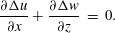 $$\begin{eqnarray}\displaystyle {\displaystyle \frac{\unicode[STIX]{x2202}\unicode[STIX]{x0394}u}{\unicode[STIX]{x2202}x}}+{\displaystyle \frac{\unicode[STIX]{x2202}\unicode[STIX]{x0394}w}{\unicode[STIX]{x2202}z}} & = & \displaystyle 0.\end{eqnarray}$$
It should be noted that in (2.11a
) we have neglected the term
 $\unicode[STIX]{x0394}u\unicode[STIX]{x2202}U/\unicode[STIX]{x2202}x$
compared with the term
 $U\unicode[STIX]{x2202}\unicode[STIX]{x0394}u/\unicode[STIX]{x2202}x$
, as the streamwise recovery of the wake is relatively small.
In the upper layer, where
 $\unicode[STIX]{x2202}U/\unicode[STIX]{x2202}z$
is small, the above equations reduce to a Laplace equation for
 $\unicode[STIX]{x0394}w$
(i.e.
 $\unicode[STIX]{x1D6FB}^{2}(\unicode[STIX]{x0394}w)=0$
). This equation can be solved, and from continuity, the solution for
 $\unicode[STIX]{x0394}u$
is obtained:
 $$\begin{eqnarray}\unicode[STIX]{x0394}u^{U}=\left({\displaystyle \frac{H}{L}}\right)\left({\displaystyle \frac{1}{\unicode[STIX]{x03C0}}}\right)\int _{-\infty }^{\infty }{\displaystyle \frac{(\unicode[STIX]{x2202}f/\unicode[STIX]{x2202}x)(\unicode[STIX]{x1D709}/L)(x-\unicode[STIX]{x1D709})\text{d}\unicode[STIX]{x1D709}}{(x-\unicode[STIX]{x1D709})^{2}+z^{2}}},\end{eqnarray}$$
where
 $\unicode[STIX]{x1D709}$
is a dummy variable for integration, and the superscript
 $U$
indicates a quantity in the upper layer. Furthermore, we can now express the total
 $\overline{u}$
velocity for both the wake and no-wake case:
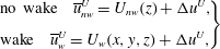 $$\begin{eqnarray}\left.\begin{array}{@{}l@{}}\displaystyle \text{no wake}\quad \overline{u}_{nw}^{U}=U_{nw}(z)+\unicode[STIX]{x0394}u^{U},\\[8.0pt] \displaystyle \text{wake}\quad \overline{u}_{w}^{U}=U_{w}(x,y,z)+\unicode[STIX]{x0394}u^{U},\end{array}\!\!\!\right\}\end{eqnarray}$$
where the subscripts
 $w$
and
 $nw$
indicate wake (i.e. when the turbine is present) and no-wake (i.e. the case without turbine) cases, respectively.
2.3.3 Middle layer
The height of the middle layer
 $h_{m}$
is considered to be
 $h_{m}=L$
for long hills (
 $L>H$
) which is the case in the current study (Hunt et al.
Reference Hunt, Leibovich and Richards1988). In the middle layer, the pressure is taken to be varying only in the horizontal directions (i.e.
 $\unicode[STIX]{x2202}\unicode[STIX]{x0394}p_{t}/\unicode[STIX]{x2202}Z=0$
). We then obtain the following equation for the streamwise and vertical velocities:
 $$\begin{eqnarray}\overline{u}_{t}{\displaystyle \frac{\unicode[STIX]{x2202}^{2}\overline{w}_{t}}{\unicode[STIX]{x2202}Z^{2}}}-\overline{w}_{t}{\displaystyle \frac{\unicode[STIX]{x2202}^{2}\overline{u}_{t}}{\unicode[STIX]{x2202}Z^{2}}}=2{\displaystyle \frac{\unicode[STIX]{x2202}}{\unicode[STIX]{x2202}Z}}\left[\overline{v}_{t}{\displaystyle \frac{\unicode[STIX]{x2202}\overline{u}_{t}}{\unicode[STIX]{x2202}y}}\right].\end{eqnarray}$$
In the case of a base flow which is only a function of
 $z$
(e.g. in the no-wake case), the right-hand side of (2.14) is equal to zero (because
 $\unicode[STIX]{x2202}U/\unicode[STIX]{x2202}y=0$
). However, in the case of a wake flow, not only
 $\unicode[STIX]{x2202}U/\unicode[STIX]{x2202}y\neq 0$
, but also it is not negligible; in fact, it has the same order of magnitude as
 $\unicode[STIX]{x2202}U/\unicode[STIX]{x2202}z$
. Nevertheless, for a 2-D hill, it is a good assumption to consider
 $\overline{v}_{t}$
as negligible. Therefore, in this case we can still neglect this term, and the equation becomes
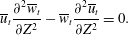 $$\begin{eqnarray}\overline{u}_{t}{\displaystyle \frac{\unicode[STIX]{x2202}^{2}\overline{w}_{t}}{\unicode[STIX]{x2202}Z^{2}}}-\overline{w}_{t}{\displaystyle \frac{\unicode[STIX]{x2202}^{2}\overline{u}_{t}}{\unicode[STIX]{x2202}Z^{2}}}=0.\end{eqnarray}$$
After considering
 $\overline{u}_{t}\approx U$
the above equation becomes an ODE, which can be solved for
 $\overline{w}_{t}$
. Next, by continuity,
 $\unicode[STIX]{x0394}u_{t}$
can be obtained (the details can be found in Hunt et al.
Reference Hunt, Leibovich and Richards1988):
 $$\begin{eqnarray}\left.\begin{array}{@{}l@{}}\displaystyle \unicode[STIX]{x0394}u_{t}=-[A(x)-Hf]{\displaystyle \frac{\unicode[STIX]{x2202}U(x,y,Z)}{\unicode[STIX]{x2202}Z}}-{\displaystyle \frac{B(x,y)J(x,y,Z)}{U(x,y,Z)}},\\[8.0pt] \displaystyle \text{where}\quad J(x,y,Z)=1+U(x,y,Z){\displaystyle \frac{\unicode[STIX]{x2202}U(x,y,Z)}{\unicode[STIX]{x2202}Z}}\int _{Z_{l}}^{Z}{\displaystyle \frac{\text{d}\unicode[STIX]{x1D701}}{U^{2}(x,y,\unicode[STIX]{x1D701})}},\end{array}\!\!\!\right\}\end{eqnarray}$$
where
 $Z_{l}=\sqrt{lz_{o}}$
,
 $l$
is the thickness of the inner region (see above for determination of the value of
 $l$
) and
 $\unicode[STIX]{x1D701}$
is a dummy variable for the integration. The functions
 $A(x)$
and
 $B(x,y)$
will be found from the matching of the middle layer to the inner region and upper layer, respectively. Matching
 $\overline{w}$
between the middle layer and inner region results in
 $A(x)=Hf(x/L)$
(Hunt et al.
Reference Hunt, Leibovich and Richards1988). Now we match
 $\overline{u}$
between the middle and upper layers in a direct manner which is different from the approximate matching of Hunt et al. (Reference Hunt, Leibovich and Richards1988). For this purpose, we equate
 $\overline{u}$
at
 $z=h_{m}+Hf(x/L)$
and
 $\overline{u}_{t}$
at
 $Z=h_{m}$
, and after some manipulations, we obtain the following relation for
 $B(x,y)$
:
 $$\begin{eqnarray}B(x,y)={\displaystyle \frac{\left[U(x,y,Z=h_{m})-\overline{u}^{U}(x,y,z=h_{m}+Hf(x/L))\right]U(x,y,Z=h_{m})}{J(x,y,Z=h_{m})}}.\end{eqnarray}$$
Now, the only remaining part of the model that needs to be determined is the mean velocity distribution
 $U(x,y,z)$
of the base flow. For the case of the flow without the turbine, we consider a logarithmic profile, and for the case of wake flow behind a wind turbine, we consider a velocity deficit function calculated in § 2.2:
 $$\begin{eqnarray}\left.\begin{array}{@{}l@{}}\displaystyle \text{no wake}\quad U(x,y,z)=U_{nw}(z)={\displaystyle \frac{u_{\ast }}{\unicode[STIX]{x1D705}}}\ln (z/z_{o}),\\[8.0pt] \displaystyle \text{wake}\quad U(x,y,z)=U_{w}(x,y,z)=U_{nw}(z)\{1-C(x)\text{e}^{-(r^{2}/2\unicode[STIX]{x1D6FF}^{2})}\},\end{array}\!\!\!\right\}\end{eqnarray}$$
where
 $C(x)$
and
 $\unicode[STIX]{x1D6FF}(x)$
were already determined in § 2.2.
By using the above relations for the base flow in (2.16), we are able to obtain
 $\unicode[STIX]{x0394}u_{t}$
in the middle layer for both the wake and no-wake cases. Next, by using equation (2.9a
), we can get the total perturbed streamwise velocity
 $\overline{u}_{t}$
:
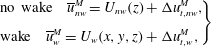 $$\begin{eqnarray}\left.\begin{array}{@{}l@{}}\displaystyle \text{no wake}\quad \overline{u}_{nw}^{M}=U_{nw}(z)+\unicode[STIX]{x0394}u_{t,nw}^{M},\\[8.0pt] \displaystyle \text{wake}\quad \overline{u}_{w}^{M}=U_{w}(x,y,z)+\unicode[STIX]{x0394}u_{t,w}^{M},\end{array}\!\!\!\right\}\end{eqnarray}$$
where the superscript
 $M$
indicates a quantity in the middle layer. The velocity deficit is then obtained as
 $$\begin{eqnarray}\overline{u}_{def}(x,y,Z)=\overline{u}_{nw}^{M}-\overline{u}_{w}^{M}.\end{eqnarray}$$
For the no-wake case (i.e. flow over a hill without a turbine), normally the upper layer solution is used (i.e.
 $\overline{u}_{nw}^{U}$
in (2.13)). This is an industry standard choice and normally results in more accurate results than the middle layer solution for the no-wake case (for example in the orographic model used in the Wind Atlas Analysis and Application Program (WAsP): Bowen & Mortensen Reference Bowen and Mortensen2004). In this case, in order to be consistent between the wake and the no-wake cases, we can define
 $\overline{u}_{w}^{UM}$
in terms of the upper layer solution for the no-wake case and the velocity deficit of (2.20):
 $$\begin{eqnarray}\overline{u}_{w}^{UM}(x,y,Z)=\overline{u}_{nw}^{U}(x,y,Z+Hf(x/L))-\overline{u}_{def}(x,y,Z).\end{eqnarray}$$
Finally, the trajectory of the wake centre is defined as
 $$\begin{eqnarray}Z_{c}(x)=\underset{Z}{\text{argmax}}\left(\overline{u}_{def}(x,y_{h},Z)\right),\end{eqnarray}$$
where
 $y_{h}$
is the
 $y$
-position of the turbine hub.
Finally, note that a clear step-by-step summary of the model (including inputs, outputs and the procedure) together with a nomenclature of key variables can be consulted by the interested reader in appendix A.
3 Numerical experiments
For the purpose of acquiring new and more detailed insight into the problem at hand and also for testing the above-described modelling framework, we perform some numerical experiments using LES. In this section, the LES set-up and some key qualitative results are presented.
3.1 LES set-up
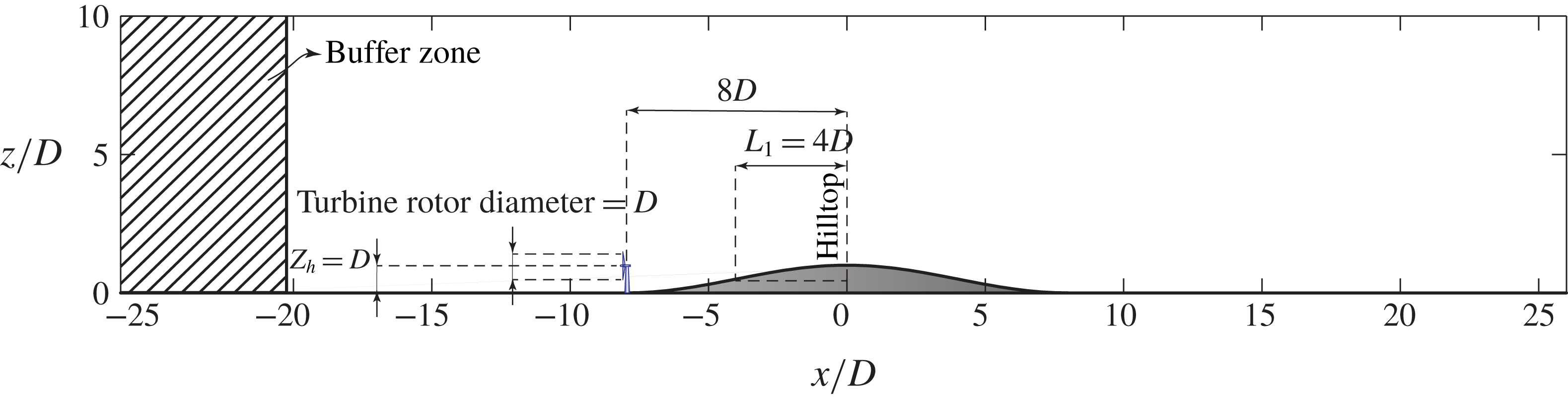
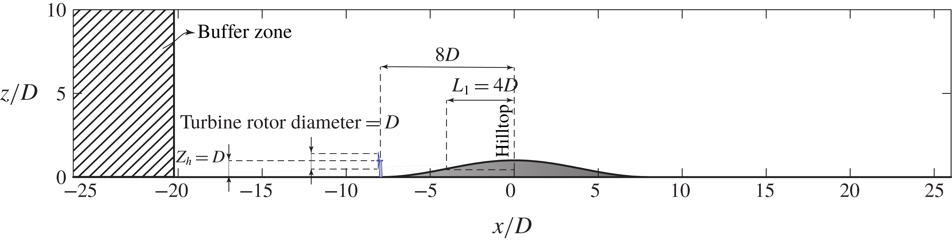
In our numerical experiments, we simulate the flow through a turbine which is sited upstream of a 2-D hill. The hub height and the diameter of the turbine are chosen to be equal, as these two values are close together also in real wind turbines. Regarding the dimensions of the hill, our aim is to have a hill of significant height with respect to the turbine dimensions. For this purpose, we have taken the hill height to be just equal to hub height of the turbine.
The simulation domain is shown in figure 4. The terrain profile is given by the following equation:
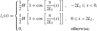 $$\begin{eqnarray}z_{s}(x)=\left\{\begin{array}{@{}ll@{}}{\displaystyle \frac{1}{2}}H\left[1+\cos \left[{\displaystyle \frac{\unicode[STIX]{x03C0}}{2L_{1}}}(x)\right]\right], & -2L_{1}\leqslant x<0,\\ {\displaystyle \frac{1}{2}}H\left[1+\cos \left[{\displaystyle \frac{\unicode[STIX]{x03C0}}{2L_{2}}}(x)\right]\right], & 0\leqslant x<2L_{2},\\ 0, & \text{otherwise},\end{array}\right.\end{eqnarray}$$
where
 $z_{s}$
is the height of the terrain, the origin of
 $x$
(as shown in figure 4) is the position of the hilltop,
 $H$
is the hill height which has the value of
 $H=D$
, and
 $L_{1}$
and
 $L_{2}$
are the half-lengths of the hill for the windward and leeward sections, respectively. Regarding the values of
 $L_{1}$
and
 $L_{2}$
, we should keep in mind that the hill is required not to be too steep for application of the framework of § 2. Accordingly, a value of
 $4D$
is chosen for
 $L_{1}$
. For the basic symmetrical hill, which is the basic case in this paper, we have
 $L_{2}=L_{1}$
; however, we will investigate different values of
 $L_{2}$
in § 4. Moreover, the thrust coefficient of the turbine is set to
 $C_{T}=0.7$
.
Domain of the simulations.
In our LES, the filtered incompressible Navier–Stokes equations (for a neutrally stratified atmospheric boundary layer) are solved, which can be written in rotational form as
 $$\begin{eqnarray}\displaystyle & \displaystyle {\displaystyle \frac{\unicode[STIX]{x2202}\widetilde{u}_{i}}{\unicode[STIX]{x2202}x_{i}}}=0, & \displaystyle\end{eqnarray}$$
 $$\begin{eqnarray}\displaystyle & \displaystyle {\displaystyle \frac{\unicode[STIX]{x2202}\widetilde{u}_{i}}{\unicode[STIX]{x2202}t}}+\widetilde{u}_{j}\left({\displaystyle \frac{\unicode[STIX]{x2202}\widetilde{u}_{i}}{\unicode[STIX]{x2202}x_{j}}}-{\displaystyle \frac{\unicode[STIX]{x2202}\widetilde{u}_{j}}{\unicode[STIX]{x2202}x_{i}}}\right)=-{\displaystyle \frac{\unicode[STIX]{x2202}\tilde{p}^{\ast }}{\unicode[STIX]{x2202}x_{i}}}-{\displaystyle \frac{\unicode[STIX]{x2202}\unicode[STIX]{x1D70F}_{ij}}{\unicode[STIX]{x2202}x_{j}}}-{\displaystyle \frac{f_{i}}{\unicode[STIX]{x1D70C}}}+F_{p}\unicode[STIX]{x1D6FF}_{i1}, & \displaystyle\end{eqnarray}$$
where the tilde represents a three-dimensional spatial filtering operation,
 $\widetilde{u}_{i}$
is the filtered velocity in the
 $i$
-direction (with
 $i=1,2,3$
corresponding to the streamwise (
 $x$
), spanwise (
 $y$
) and vertical (
 $z$
) directions, respectively),
 $\tilde{p}^{\ast }=\widetilde{p}/\unicode[STIX]{x1D70C}+1/2\widetilde{u}_{i}\widetilde{u}_{i}$
is the modified kinematic pressure where
 $\widetilde{p}$
is the filtered pressure,
 $\unicode[STIX]{x1D70F}_{ij}=\widetilde{u_{i}u_{j}}-\widetilde{u_{i}}\widetilde{u_{j}}$
is the kinematic subgrid-scale (SGS) stress,
 $f_{i}$
is a body force (per unit volume) used to model the effects of the turbine on the flow,
 $F_{p}$
acts as the driving force of the flow (in the streamwise-periodic case) and
 $\unicode[STIX]{x1D70C}$
is the constant fluid density. In this paper,
 $u$
,
 $v$
and
 $w$
notations are also used for the
 $u_{1}$
,
 $u_{2}$
and
 $u_{3}$
velocity components, respectively. Regarding the parametrization of the SGS stresses, the Lagrangian scale-dependent dynamic model (Stoll & Porté-Agel Reference Stoll and Porté-Agel2006) is used.
The turbine forces acting on the flow are modelled using the standard actuator disk model (Wu & Porté-Agel Reference Wu and Porté-Agel2011). The hilly terrain at the bottom of the domain is treated by using a terrain-following coordinate system, whose details are described in Shamsoddin & Porté-Agel (Reference Shamsoddin and Porté-Agel2017a ). The horizontal boundary conditions are mathematically periodic. For the upper boundary, an impermeable free-stress boundary condition is assigned, and for the lower boundary, the instantaneous surface shear stress is calculated using the Monin–Obukhov similarity theory (which for the neutral case of this study simply reduces to the log law). To eliminate the periodicity of the flow in the streamwise direction, a buffer zone technique is employed, in which we feed an inflow field to our simulation. This inflow field is obtained from an offline precursory simulation (whose domain size and grid size are the same as in the final simulations) over a flat terrain (Tseng, Meneveau & Parlange Reference Tseng, Meneveau and Parlange2006; Wan & Porté-Agel Reference Wan and Porté-Agel2011; Wu & Porté-Agel Reference Wu and Porté-Agel2011; Shamsoddin & Porté-Agel Reference Shamsoddin and Porté-Agel2014, Reference Shamsoddin and Porté-Agel2016, Reference Shamsoddin and Porté-Agel2017a ). The details of the LES framework, its numerics and the SGS model are described, for instance, in Albertson & Parlange (Reference Albertson and Parlange1999), Porté-Agel, Meneveau & Parlange (Reference Porté-Agel, Meneveau and Parlange2000), Stoll & Porté-Agel (Reference Stoll and Porté-Agel2006), Wan, Porté-Agel & Stoll (Reference Wan, Porté-Agel and Stoll2007), Porté-Agel et al. (Reference Porté-Agel, Wu, Lu and Conzemius2011) and Shamsoddin & Porté-Agel (Reference Shamsoddin and Porté-Agel2017a ).
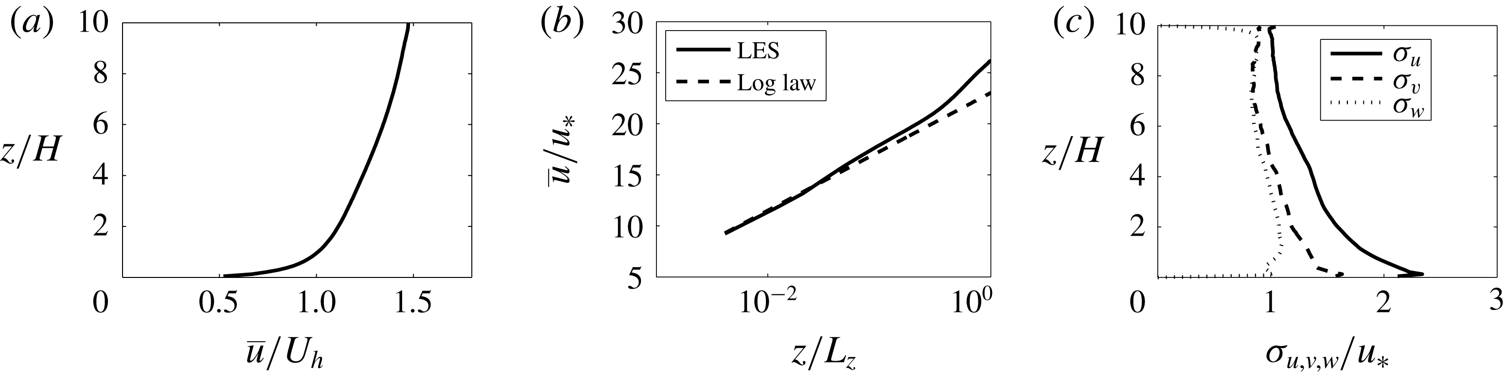
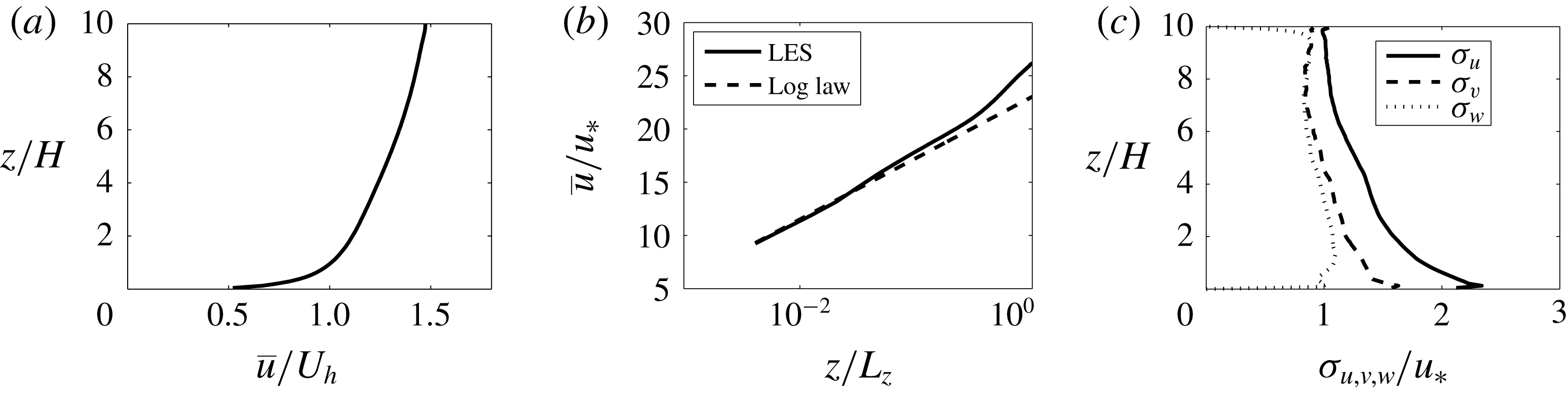
Inflow characteristics: (a) vertical profile of the mean streamwise velocity (linear scale), (b) vertical profile of the mean streamwise velocity compared to a log-law profile (horizontal axis in logarithmic scale), (c) vertical profiles of the normalized standard deviation of the streamwise, spanwise and vertical velocities.
The dimensions of the domain are
 $52.5D$
,
 $8.75D$
and
 $10D$
in the
 $x$
-,
 $y$
- and
 $z$
-directions, respectively. The number of grid points in the
 $x$
-,
 $y$
- and
 $z$
-directions are, respectively, 210, 60 and 122. Moreover, the ratio of the surface roughness length to the domain height (i.e.
 $10D$
) is set to
 $10^{-4}$
which is a typical value for farmland. The inflow characteristics (corresponding to a friction velocity of
 $u_{\ast }=0.5~\text{ms}^{-1}$
) are shown in figure 5. It is noteworthy that we ran another simulation with a domain height twice as large as the current one (i.e.
 $20D$
instead of
 $10D$
), to check if the height of the domain is large enough with respect to the hill height in order to have a negligible blockage effect. By comparing the velocity profiles of the two simulations over the hill, we observed that they are almost identical in the regions that we are interested in (i.e. the region surrounding the turbine wake). Hence, we conclude that the height of the domain is sufficiently large. Furthermore, regarding the blockage effect of the turbine, it should be noted that the blockage ratio caused by the turbine in the domain is 0.009, which can safely be considered as negligible based on Segalini & Inghels (Reference Segalini and Inghels2014).
The accuracy of this LES framework has been tested in several validation studies: the validation of the actuator disk model was performed in Wu & Porté-Agel (Reference Wu and Porté-Agel2011) and Porté-Agel et al. (Reference Porté-Agel, Wu, Lu and Conzemius2011) and the validation of the coordinate transformation technique was carried out in Wan et al. (Reference Wan, Porté-Agel and Stoll2007). On top of these, the combined application of the actuator disk and coordinate transformation methods was validated in Shamsoddin & Porté-Agel (Reference Shamsoddin and Porté-Agel2017a ). The chosen resolution of the grid is well within the range that has been previously shown to result in grid-independent results for the cases of application of the coordinate transformation (see Wan et al. (Reference Wan, Porté-Agel and Stoll2007, § 3)) and flow through actuator disks (see Wu & Porté-Agel (Reference Wu and Porté-Agel2011, § 4), and Wu & Porté-Agel (Reference Wu and Porté-Agel2013, § 4.1)), and the case of the combined application of the coordinate transformation and the actuator disks (Shamsoddin & Porté-Agel Reference Shamsoddin and Porté-Agel2017a ).
3.2 An overview of LES results
3.2.1 Mean velocity field
Contours of the normalized mean streamwise velocity (
 $\overline{u}/U_{h}$
) in the
 $xz$
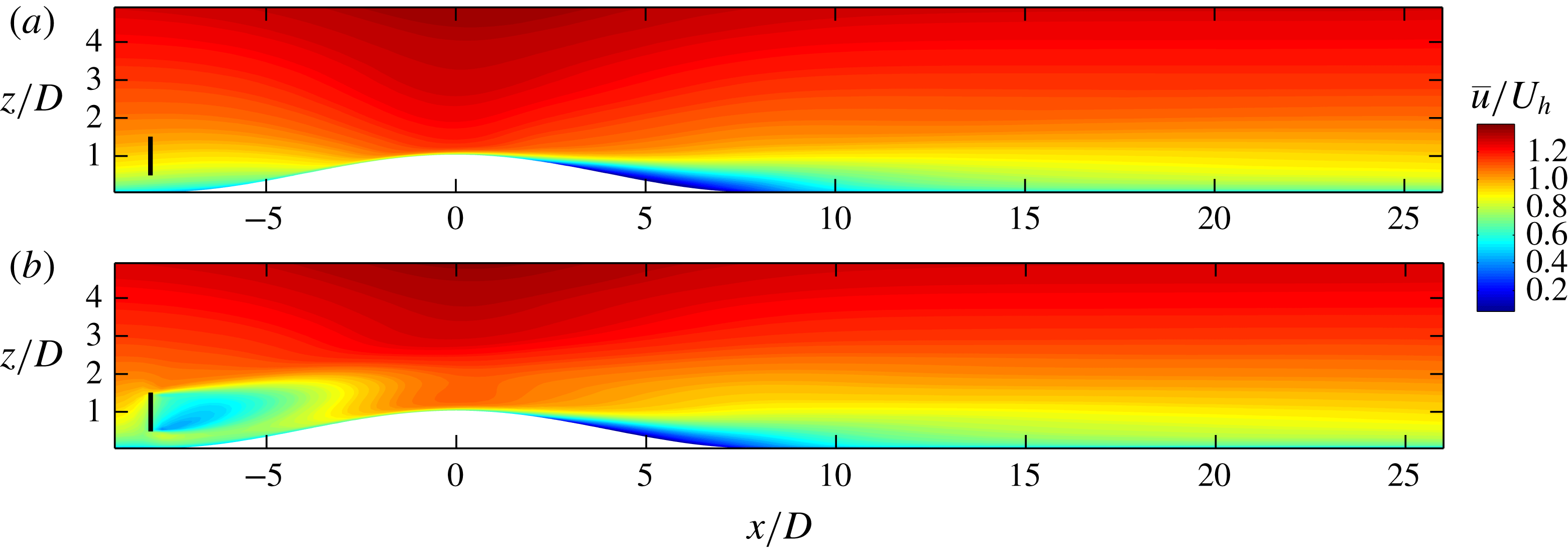
-plane going through the centre of the turbine. (a) No-wake case. (b) Turbine case.
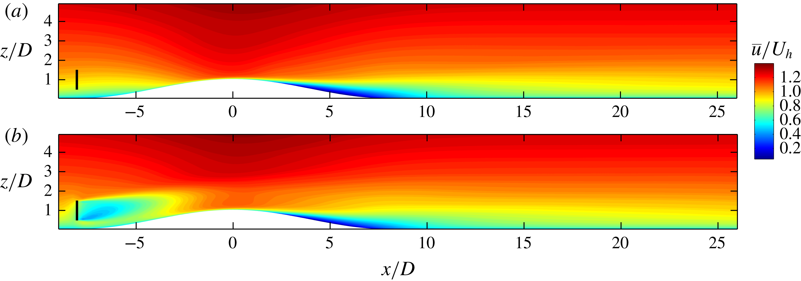
Figure 6 shows the contours of the normalized streamwise component of the mean velocity for both wake and no-wake cases. The velocities are normalized by the velocity at hub height far upwind of the hill
 $U_{h}$
(i.e. over a flat terrain). To isolate the turbine wake, we define the velocity deficit as follows:
 $$\begin{eqnarray}\overline{u}_{def}(x,y,z)=\overline{u}_{nw}(x,y,z)-\overline{u}_{w}(x,y,z),\end{eqnarray}$$
where the subscripts
 $w$
and
 $nw$
indicate wake and no-wake cases, respectively. In other words, to obtain the velocity deficit at a given point, we subtract the velocity of that point in the wake case from the velocity of the same point in the no-wake case. Traditionally, in turbine wake flows over a flat terrain, the velocity deficit is defined based on the incoming velocity profile; however, in our case here, the incoming flow is perturbed both by the hill and the turbine, therefore the traditional definition of velocity deficit is not able to isolate the effect of the turbine (i.e. the turbine wake). It is noteworthy to mention that the definition in (3.4) is reduced to the traditional definition of velocity deficit in the case of turbine wake flow over a flat terrain.
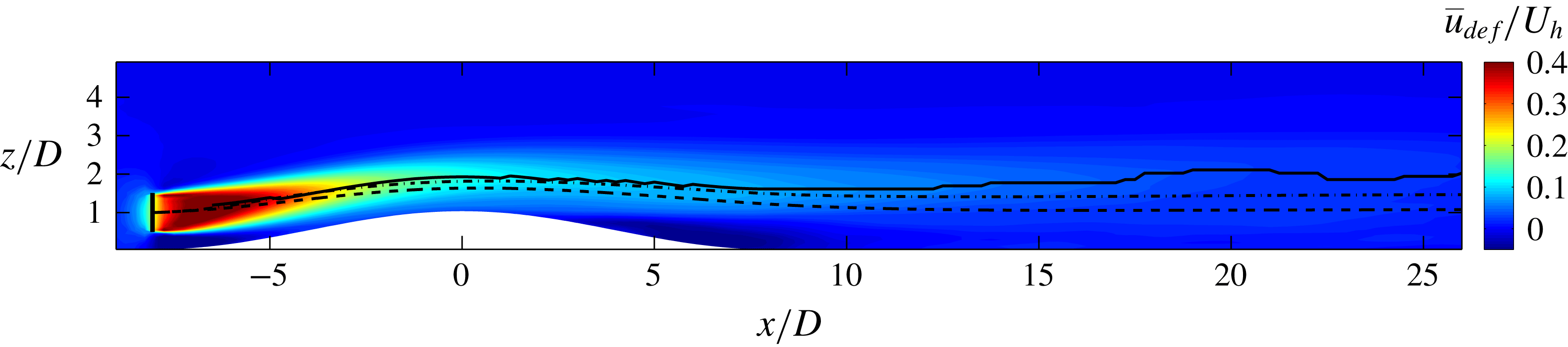
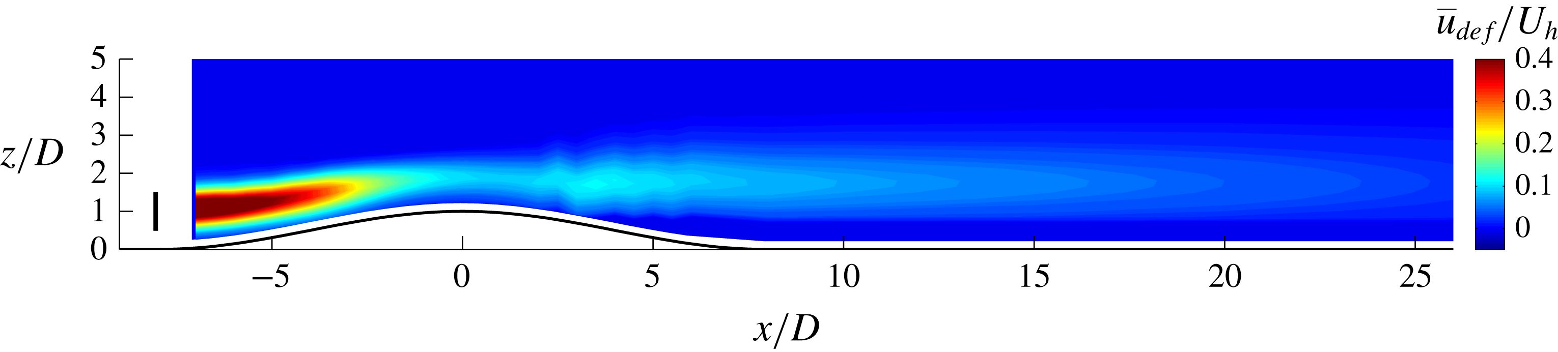
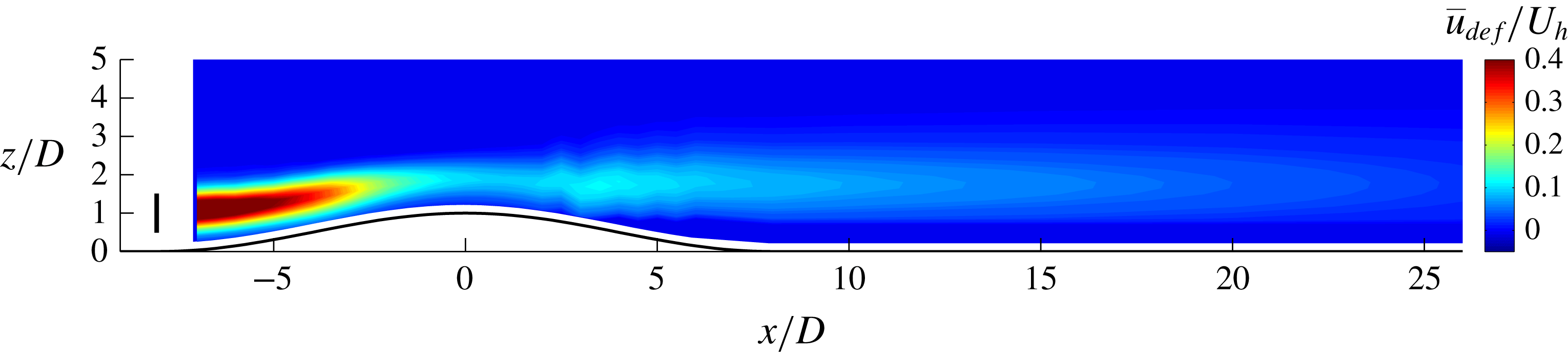
Figure 7 shows the normalized velocity deficit in the vertical midplane of the domain. The turbine wake and the wake centre trajectory (black solid line) can be seen in this figure. The wake centre trajectory is defined as
 $$\begin{eqnarray}z_{c}(x)=\underset{z}{\text{argmax}}\left(\overline{u}_{def}(x,y_{h},z)\right),\end{eqnarray}$$
where
 $z_{c}(x)$
is the
 $z$
-coordinate of the wake centre as a function of
 $x$
, and
 $y_{h}$
is the
 $y$
-coordinate of the centre of the turbine. Together with the wake centre, the mean streamlines of the flow (going through the turbine hub position) in the wake (dash-dotted line) and no-wake (dashed line) cases are also depicted in the figure. The relative position of these three lines with respect to each other is worthy of attention. The wake streamline is located above the no-wake streamline; this is because the presence of the wake decelerates the flow causing the streamlines to expand (with respect to the no-wake case) in such a way that their distance to the ground increases. This figure also shows that the wake centre trajectory is not coincident with the wake streamline; this is also observed in cross-flow jet flows (e.g. Gutmark, Ibrahim & Murugappan Reference Gutmark, Ibrahim and Murugappan2008).
In figure 7, it can be seen that behind the hill a region of negative velocity deficit is formed (this can be observed more clearly in the velocity deficit profiles of § 5). This region implies that the presence of the turbine mitigates the wind-sheltering effect of the hill. In other words, the turbine accelerates the flow on the leeward side of the hill with respect to the no-wake case.
Contours of the normalized mean streamwise velocity deficit (
 $\overline{u}_{def}/U_{h}$
) in the
 $xz$
-plane going through the centre of the turbine. Wake centre trajectory (solid line) and streamlines going through the centre of the rotor for the no-wake (dashed line) and wake (dash-dotted line) cases are also shown.
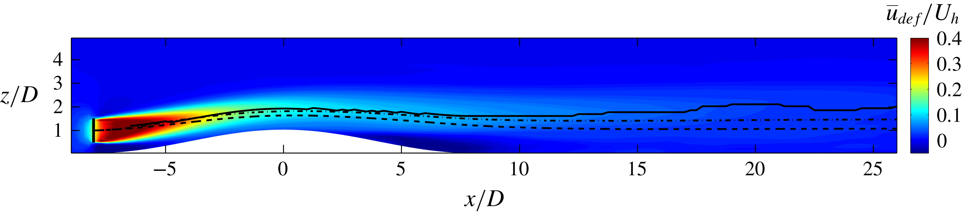
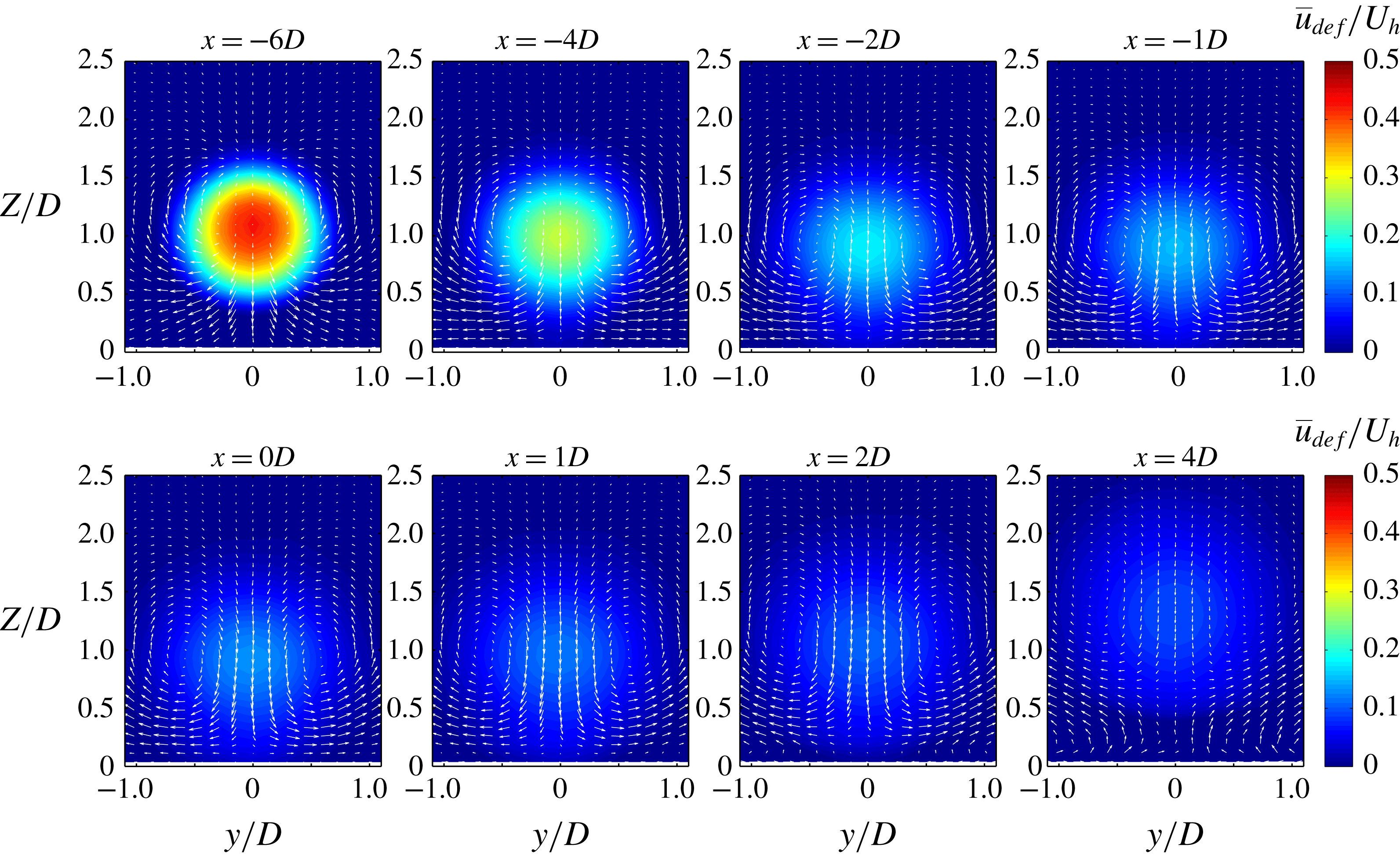
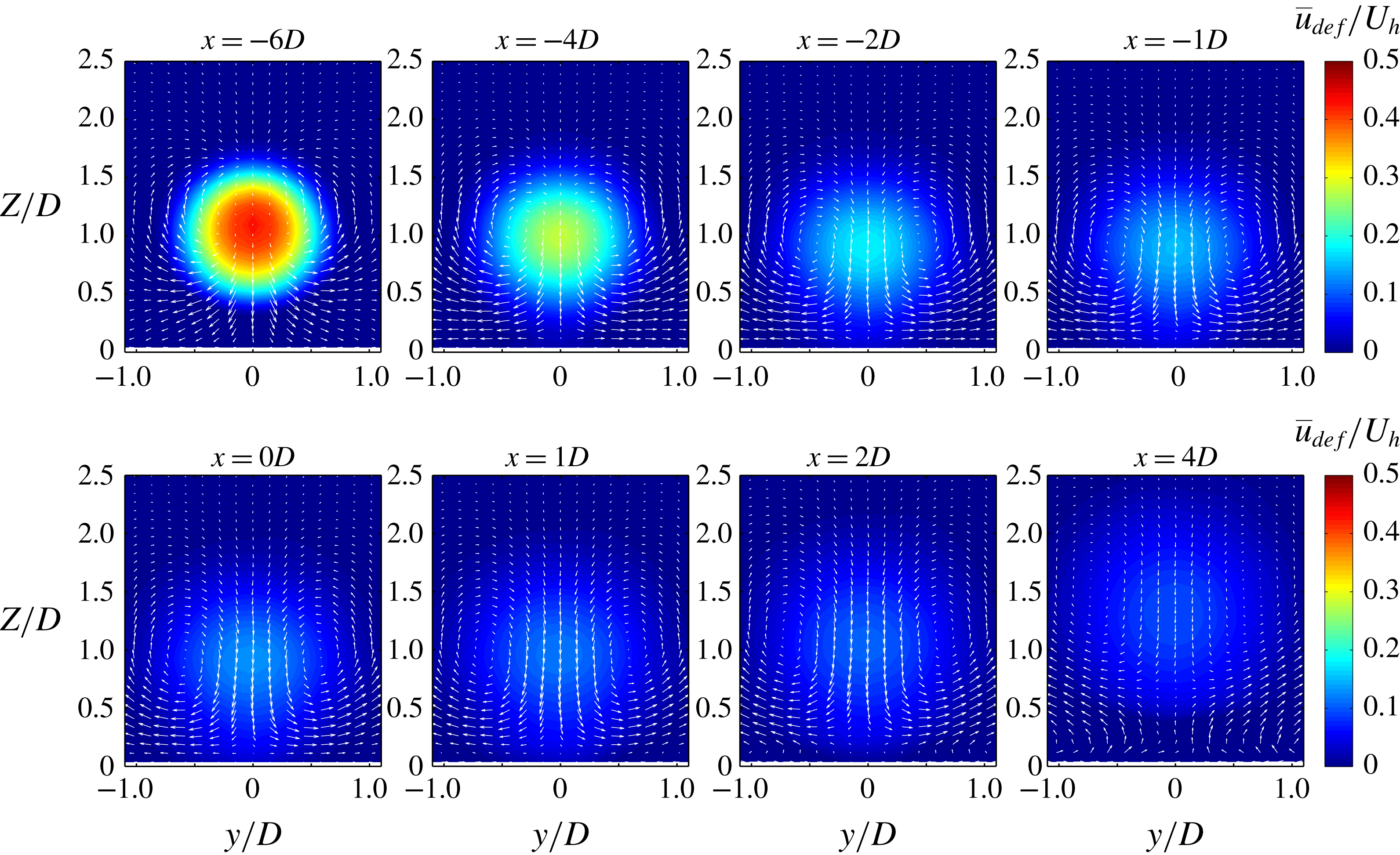
Figure 8 shows the velocity deficit in several stream-normal
 $yz$
planes. The wake cross-section seems axisymmetric as no significant asymmetry is observed. Another interesting observation in figure 8 is the behaviour of the deficit streamline vectors. These streamlines can be understood as the flow patterns for which the turbine is responsible, and are obtained based on the spanwise and vertical velocity deficits, i.e.
 $\overline{v}_{def}$
and
 $\overline{w}_{def}$
, respectively. These two quantities are defined similarly to
 $\overline{u}_{def}$
in (3.4). We see a clear pair of counter-rotating vortices at each
 $yz$
plane on the hill, whose sense of rotation is the same on the windward and leeward sides. We now try to explain the formation of these vortices. The key point here is that the turbine wake induces an upward vertical velocity in the flow over the hill (i.e.
 $-\overline{w}_{def}>0$
); this is evident in figure 8 and is consistent with the upward shift of the streamlines (in the wake case with respect to the no-wake case) in figure 7. This positive induced vertical velocity (
 $-\overline{w}_{def}$
) vanishes far from the wake in the
 $z$
-direction and is maximum somewhere in the wake region. Therefore, one can view this situation as an analogue to the cross-flow jet case, where we have a main jet (here
 $\overline{u}_{def}$
) and a cross-flow (here
 $\overline{w}_{def}$
), which is perpendicular to the jet and has a significant variation in the direction perpendicular to the jet (here
 $z$
). The formation of counter-rotating vortex pairs in cross-flow jets has been broadly observed and discussed (e.g. Kamotani & Greber Reference Kamotani and Greber1972; Fearn & Weston Reference Fearn and Weston1974; Kelso, Lim & Perry Reference Kelso, Lim and Perry1996; Cortelezzi & Karagozian Reference Cortelezzi and Karagozian2001) and the same flow structure was also observed and explained in the work of Bastankhah & Porté-Agel (Reference Bastankhah and Porté-Agel2016), who studied wakes of turbines in yawed conditions. The main difference here is that in our case these counter-rotating vortex pairs are observed in the velocity deficit field, whereas in the cross-flow jet and yawed-turbine cases, these vortex pairs are noticeable in the wake flow field itself.
Contours of the normalized mean streamwise velocity deficit (
 $\overline{u}_{def}/U_{h}$
) in several
 $yz$
planes at different streamwise positions. The white vectors show the resultant velocity from
 $\overline{v}$
and
 $\overline{w}$
.
3.2.2 Turbulence
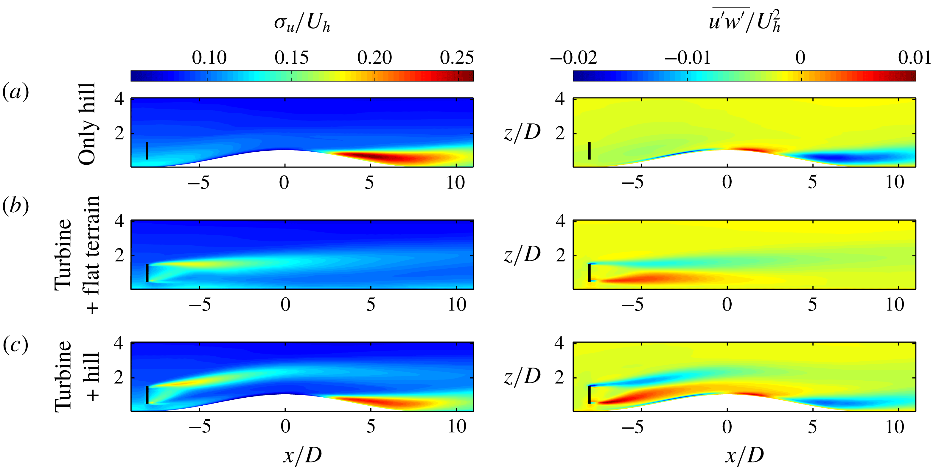
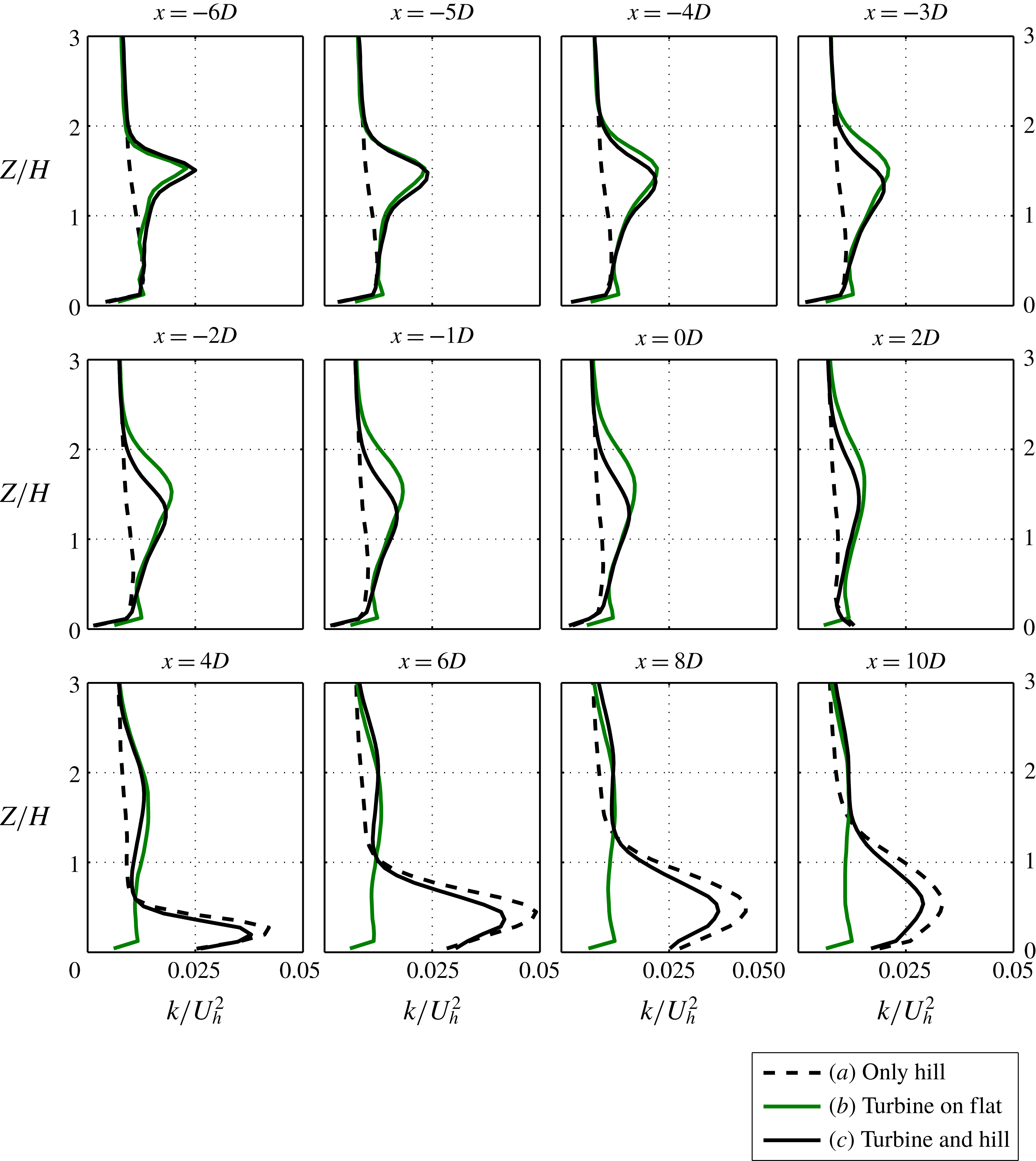
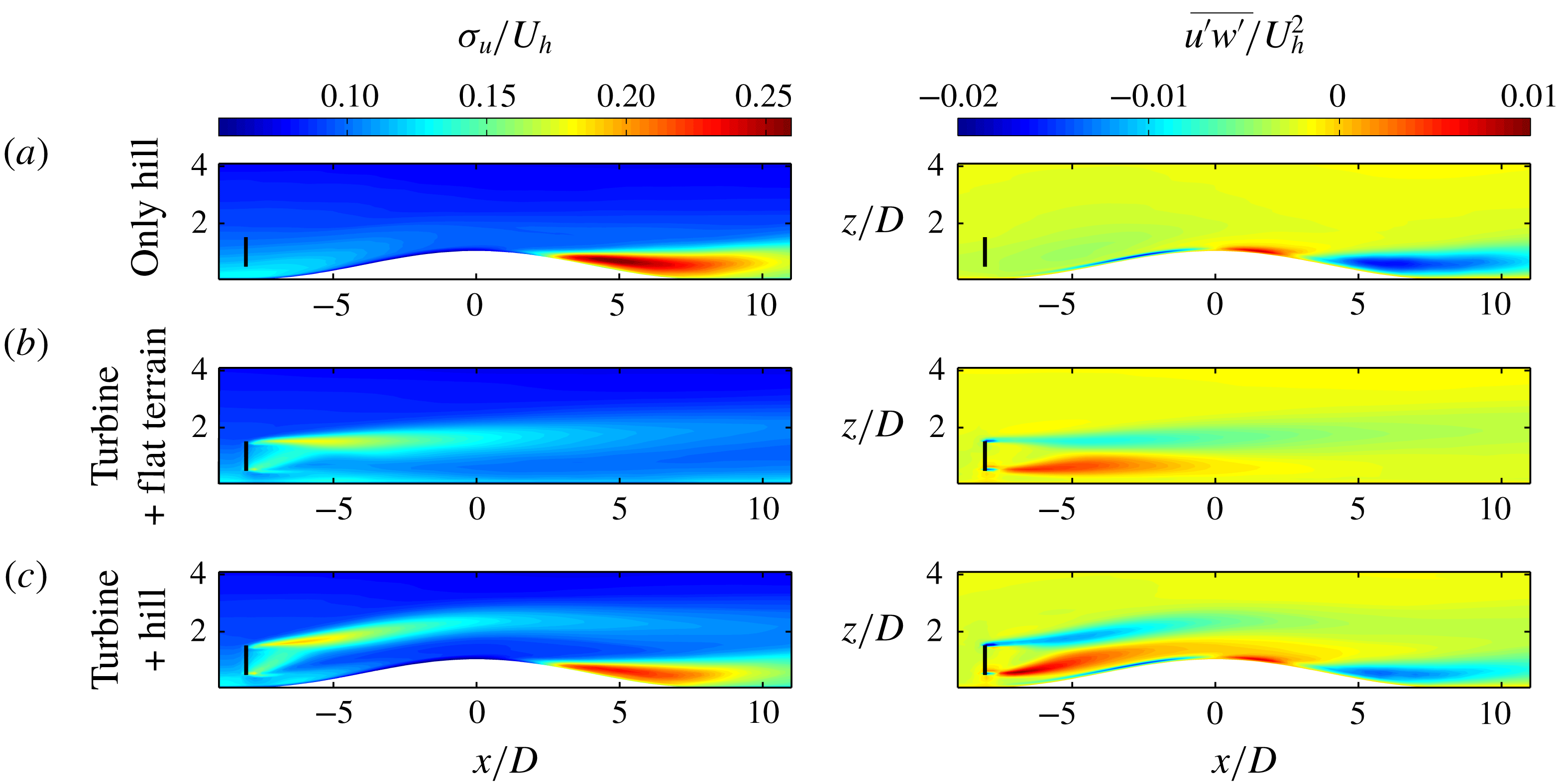
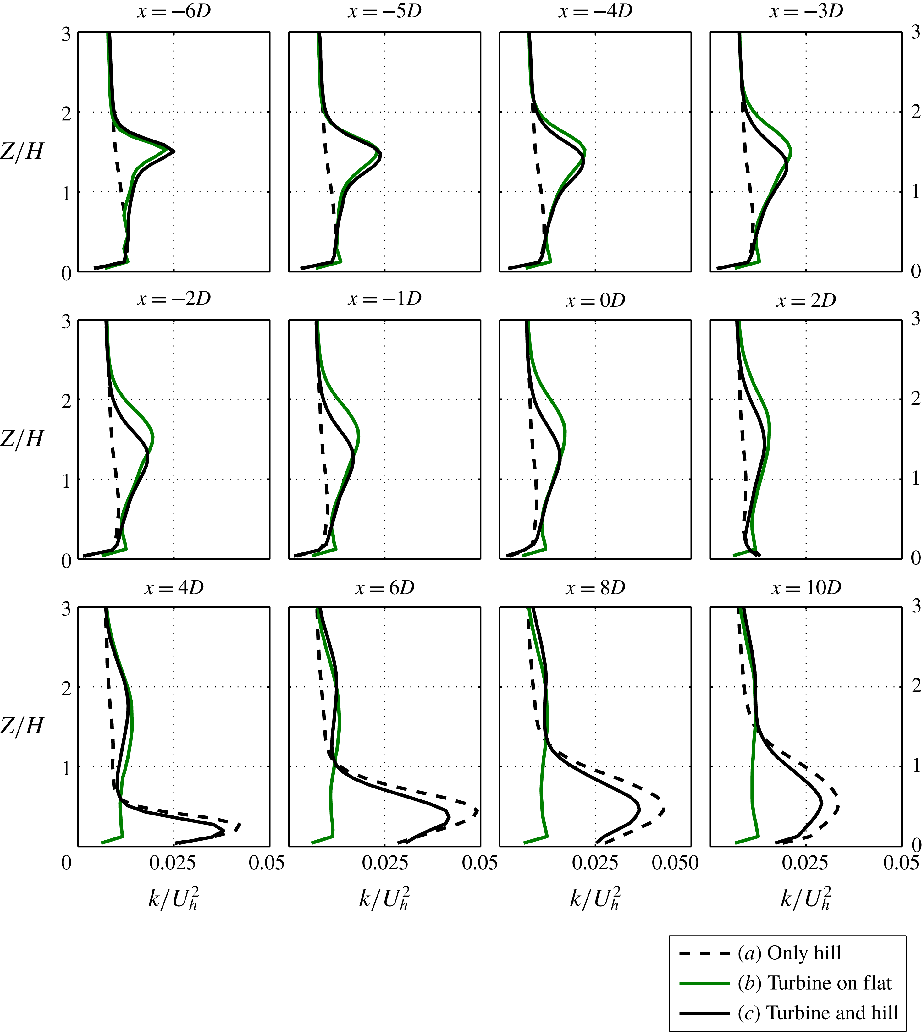
Both the hill and the turbine individually alter the turbulence structure of the incoming flow, such that they increase the turbulence level in their downwind flow. This can be seen in figure 9 for cases (a) and (b). On the other hand, when both of them are present at the same time (case (c) in figure 9), these two effects interact with each other. Besides figure 9, the vertical profiles of the turbulence kinetic energy are shown in figure 10. From these two figures some interesting observations can be made. First, we see that the turbulence level in the turbine wake is initially greater on the hilly terrain than on the flat terrain (compare cases (b) and (c) for
 $x/D$
less than approximately
 $-5$
). However, after a certain point, the turbulence level of the turbine wake on the hilly terrain drops systematically below that of flat terrain (this is especially clear before the onset of the wind-sheltering effect at around
 $x/D=2$
). This behaviour is likely to be linked to the fact that the wake recovers faster on the windward side of the hill due to the favourable pressure gradient (see §§ 2.2 and 6). Second, by inspecting the high turbulence region behind the hill, we infer that the presence of the turbine leads to a decrease in the turbulence level behind the hill (comparing cases (a) and (c)). This occurs probably because the velocity difference between the wind-sheltering ‘bubble’ behind the hill and the flow above it decreases due to the presence of the turbine wake.
Contour plots of the streamwise turbulence intensity
 $\unicode[STIX]{x1D70E}_{u}/U_{h}$
and the normalized vertical turbulent flux
 $\overline{u^{\prime }w^{\prime }}/U_{h}^{2}$
in the
 $xz$
-plane going through the centre of the turbine.
Vertical profiles of the normalized turbulence kinetic energy
 $k/U_{h}^{2}$
in the
 $xz$
-plane going through the centre of the turbine at different streamwise positions. Turbulence kinetic energy is defined as
 $k=(\unicode[STIX]{x1D70E}_{u}^{2}+\unicode[STIX]{x1D70E}_{v}^{2}+\unicode[STIX]{x1D70E}_{w}^{2})/2$
, where
 $\unicode[STIX]{x1D70E}_{u}$
, for example, is the standard deviation of
 $u$
.
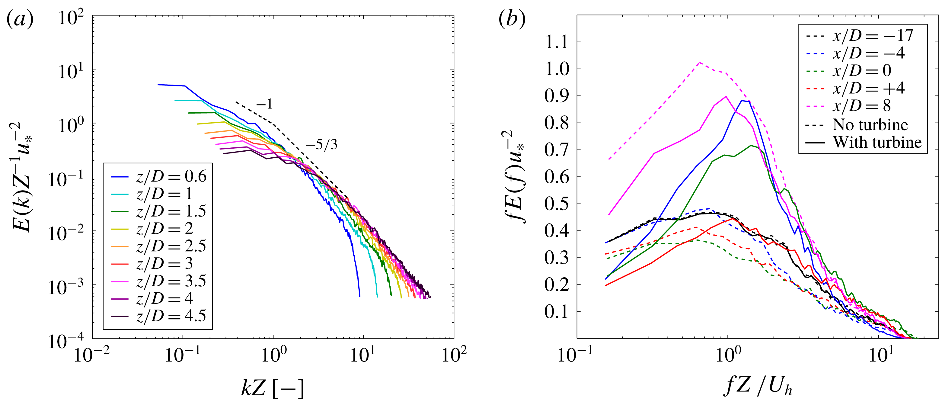
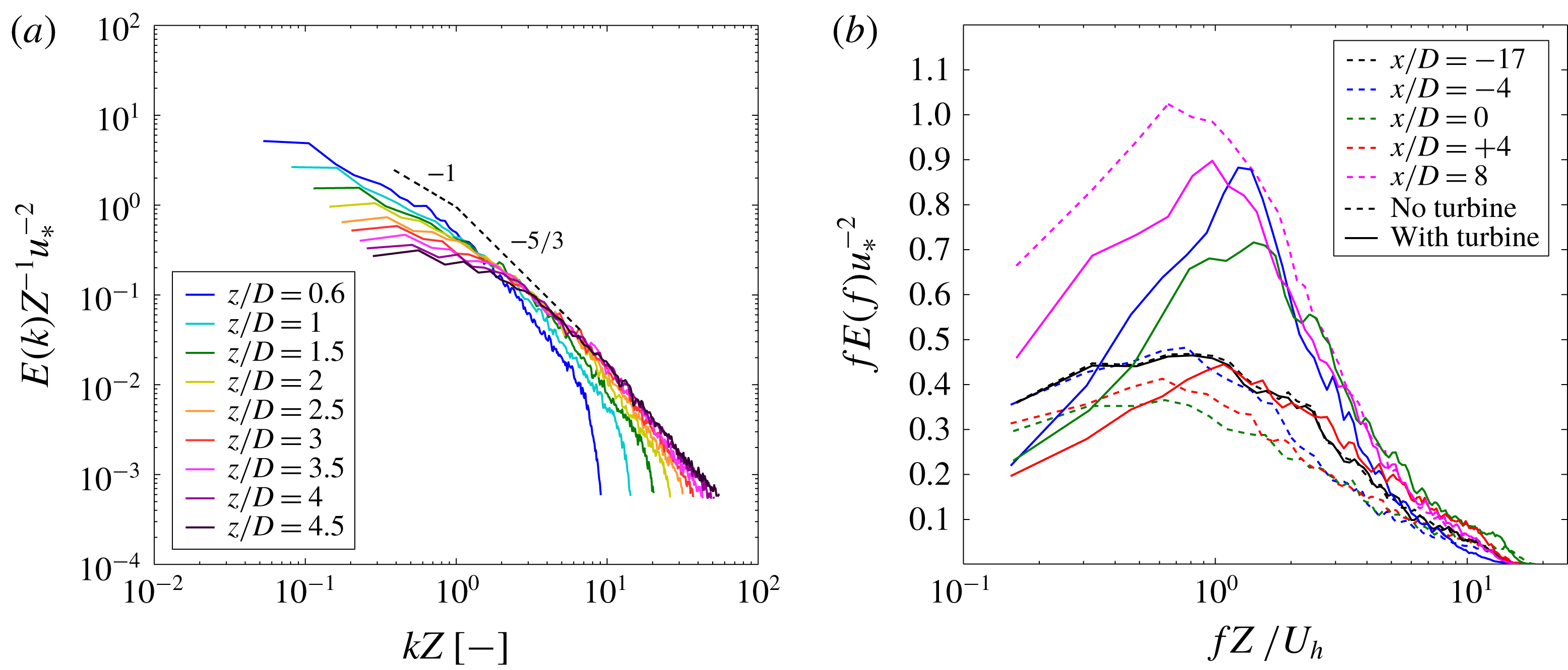
Moreover, we can take a look at the spectral behaviour of the turbulence in the flow in figure 11. Figure 11(a) shows the normalized spectral density of the streamwise velocity (
 $E(k)u_{\ast }^{-2}Z$
) as a function of
 $kZ$
, where
 $k$
is the wavenumber for the streamwise direction. This is plotted for the incoming flow in different heights using Taylor’s hypothesis. It can be seen that the energy spectrum follows the expected
 $-5/3$
law for the inertial subrange and the
 $-1$
law for the larger scales (production subrange). On the other hand, figure 11(b) shows the premultiplied spectra for different streamwise positions with respect to the hill at a constant height from the ground
 $Z=H=Z_{h}$
for cases both with and without turbine. For the case without the turbine, it can be seen that the spectra drop when we are approaching the hilltop. Then after the hilltop, and especially in the wind-sheltering bubble, they start to increase. The effect of the turbine on the spectra can be understood in two ways. First, we see that the turbine systematically shifts the peak of the spectra to the right. This means that with the presence of the turbine, the scales containing the highest amount of energy become smaller. Second, one can observe that inclusion of the turbine leads to changes in the magnitude of the energy in different scales depending on the position with respect to the hill. In line with the previous discussion on figures 9 and 10, the energy of different scales is found to generally increase on the windward side of the hill with the presence of the turbine, and conversely, it decreases in the wind-sheltering bubble.
(a) Normalized velocity spectra versus non-dimensionalized wavenumbers at different heights for the undisturbed incoming flow. (b) Premultiplied velocity spectra at height
 $H$
from the ground for different streamwise positions.
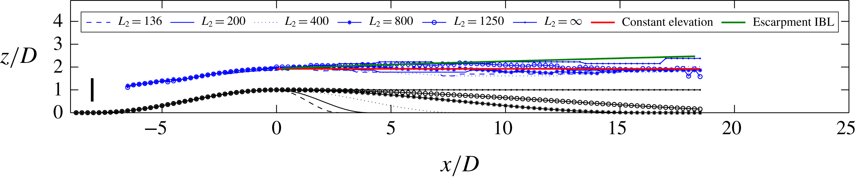
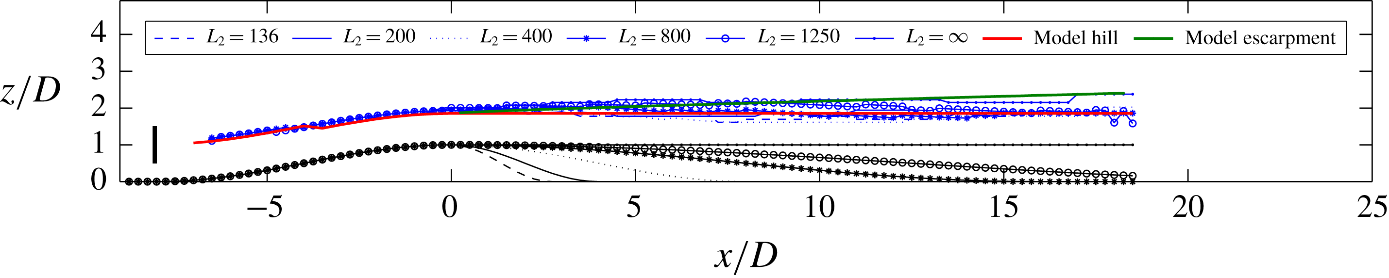
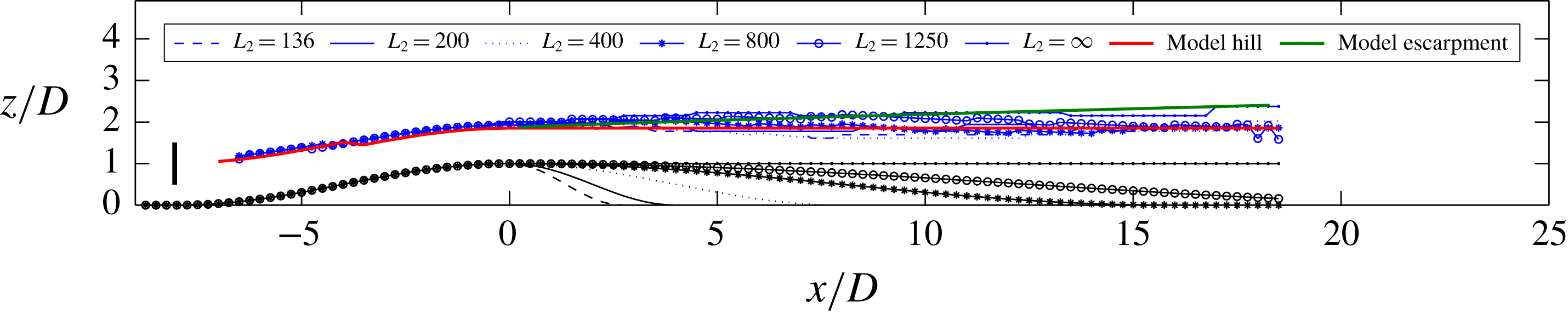
Trajectory of the turbine wake over six hills of different leeward shapes. The blue lines show the wake centre trajectory for hills of different leeward profile. Each black line shows a leeward hill profile corresponding to a blue line with the same line marker. The half-length of the leeward hill profile (
 $L_{2}$
) for each case (or line marker) is specified in the legend.

4 The wake on the leeward side of the hill
As was discussed in § 2.3, on the leeward side of the hill, we have either a separated flow or a non-separated sheltering effect of the hill which causes strong asymmetries between leeward and windward regions of the flow. The non-separated sheltering effect is easily noticeable in figure 6(a), where there is a clear asymmetry between the mean velocity distribution up- and downwind of the hilltop. This suggests that the linearized models can no longer predict well the flow downwind of the hilltop. The flow behaviour in this region is so complex that there is a scarcity of reliable simple analytical prediction models for this region in the literature, even for the case of boundary-layer flows without any wake. Herein, we attempt to analyse the wake behaviour on the leeward side, mainly based on our observations of our LES results.
The flow on the windward side up until the hilltop, which is more influenced by the windward profile of the hill, is relatively more predictable than on the leeward side. Here, we want to see how the wake trajectory on the leeward side is affected by the leeward hill profile. In other words, we would like to see how significantly the wake responds to different leeward hill profiles. For this purpose, for the same windward hill profile, we systematically change the leeward hill profile to see how the wake trajectory responds to this change. As can be seen in figure 12, we have changed the half-length of the leeward side of the hill (
 $L_{2}$
in (3.1)) from
 $1.36D$
to infinity. The extreme case of
 $L_{2}\rightarrow \infty$
, in fact, corresponds to an escarpment of the same height as the other hills. Some interesting conclusions can be made from this figure. First, we see that the leeward hill profile has almost no effect on the windward trajectory of the wake. Second, and maybe more interestingly, it can be seen that, even though the leeward hill profile has gone through significant changes, the wake trajectory above it has not changed significantly. In other words, the leeward wake trajectory is found to be only a weak function of the leeward hill profile. Especially for the hills (not for the extreme case of the escarpment), we also see that the elevation of the wake trajectory does not change considerably downwind of the hilltop.
4.1 Hills
Figure 12, besides different wake centre trajectories, also shows a red line which is a straight horizontal line whose elevation is equal to the elevation of the wake centre at the hilltop
 $z_{c}^{ht}(=z_{c}(0))$
. It can be seen that this line is a good approximation to the wake centre trajectory on the leeward side of the hill. This approximation proves to be useful because we can calculate the trajectory of the wake centre until the hilltop using the methods of § 2 and afterwards we can assume the trajectory to be a horizontal line as an approximation. Moreover, to reflect this trajectory modification in the velocity profiles on the leeward side, we can simply centre the calculated velocity deficit (i.e. 2.20) around this trajectory.
4.2 Escarpments
In the limiting case of the constant-elevation leeward hill profile (
 $L_{2}\rightarrow \infty$
), it can be seen that the wake centre ascends. This is because of the development of an internal boundary layer (IBL) on the plateau surface. Even though the flow upstream of the hill is a fully developed boundary-layer flow, it is well known that the velocity profile at the hilltop is close to being uniform (e.g. Britter et al.
Reference Britter, Hunt and Richards1981; Ishihara et al.
Reference Ishihara, Hibi and Oikawa1999; Tian et al.
Reference Tian, Ozbay, Yuan, Sarkar and Hu2013; Hyvärinen & Segalini Reference Hyvärinen and Segalini2017a
). Therefore, after the hilltop and on the plateau the boundary layer again starts to develop on the new ground. Such an approach to flow over escarpments has already been adopted, for example in Emeis, Frank & Fiedler (Reference Emeis, Frank and Fiedler1995) (or § 4.3 of Emeis Reference Emeis2013). The evolution of the IBL, which involves deceleration of the flow near the ground, requires that the streamlines diverge upwards, and as a consequence the locus of the wake centre moves upward. To predict this upward motion, we benefit from the findings in previous studies of IBLs (for a review see § 4.5.3 of Garratt Reference Garratt1994). In order to model the growth of the IBL, it is common to use an analogy between the IBL growth and diffusion of a smoke plume (Miyake Reference Miyake1965; Pasquill Reference Pasquill1972; Jackson Reference Jackson1976; Garratt Reference Garratt1990). Employing this analogy, the following equation for the upward displacement of passive particles diffusing in space from the ground can be used. The original equation was first derived by Miyake (Reference Miyake1965) and we use its modified version by Pasquill (Reference Pasquill1972):
 $$\begin{eqnarray}{\displaystyle \frac{\unicode[STIX]{x0394}Z_{p}}{z_{o}}}\left[\ln \left({\displaystyle \frac{\unicode[STIX]{x0394}Z_{p}}{z_{o}}}\right)-1\right]+1={\displaystyle \frac{A(x-x_{ht})}{z_{o}}},\end{eqnarray}$$
where
 $\unicode[STIX]{x0394}Z_{p}$
is the upward displacement of the passive particles,
 $x_{ht}$
is the
 $x$
-position of the hilltop (or the surface roughness transition) and
 $A\approx \unicode[STIX]{x1D705}^{2}$
is a constant (Pasquill Reference Pasquill1972; Garratt Reference Garratt1990). The above nonlinear equation can be solved to obtain
 $\unicode[STIX]{x0394}Z_{p}$
as a function of
 $x$
. The height of the IBL,
 $h_{b}$
, can then be obtained as
 $h_{b}=3\unicode[STIX]{x0394}Z_{p}$
(Garratt Reference Garratt1994).
If we treat the wake flow at the hilltop as a passive scalar plume and assume that its vertical displacement is close to that of a ground-level source, then we can use (4.1) as a first approximation for the upward displacement of the wake centre. For this purpose,
 $\unicode[STIX]{x0394}Z_{p}$
is replaced by
 $\unicode[STIX]{x0394}Z_{c}$
in (4.1), where
 $\unicode[STIX]{x0394}Z_{c}$
is the upward displacement of the wake centre with respect to
 $z_{c}^{ht}$
. This approximation is justifiable especially for long hills, because the velocity deficit at the hilltop becomes relatively small. In figure 12, the green line shows
 $\unicode[STIX]{x0394}Z_{c}+z_{c}^{ht}$
, where
 $\unicode[STIX]{x0394}Z_{c}$
is the solution of the (4.1). It can be seen that this method results in a good approximation for the wake trajectory on the plateau part of an escarpment.
5 Validation of the analytical model
In this section, we intend to compare the results of the analytical model presented in § 2 to those of LES for the symmetrical hill of § 3.2. As mentioned in § 2.2, the model needs the velocity at the hub-height level for the flow over the hill without the wind turbines (i.e.
 $U_{nw}^{h}(x)$
) as an input (i.e.
 $U_{b}(x)$
). There, we pointed out that to obtain
 $U_{nw}^{h}(x)$
, one can use the model developed by Jackson & Hunt (Reference Jackson and Hunt1975), i.e. equation (2.13) for the no-wake case. This is carried out for this hill and
 $U_{nw}^{h}(x)$
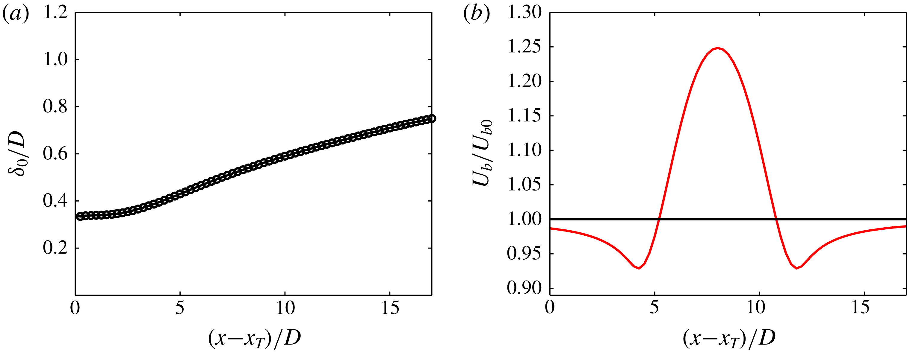
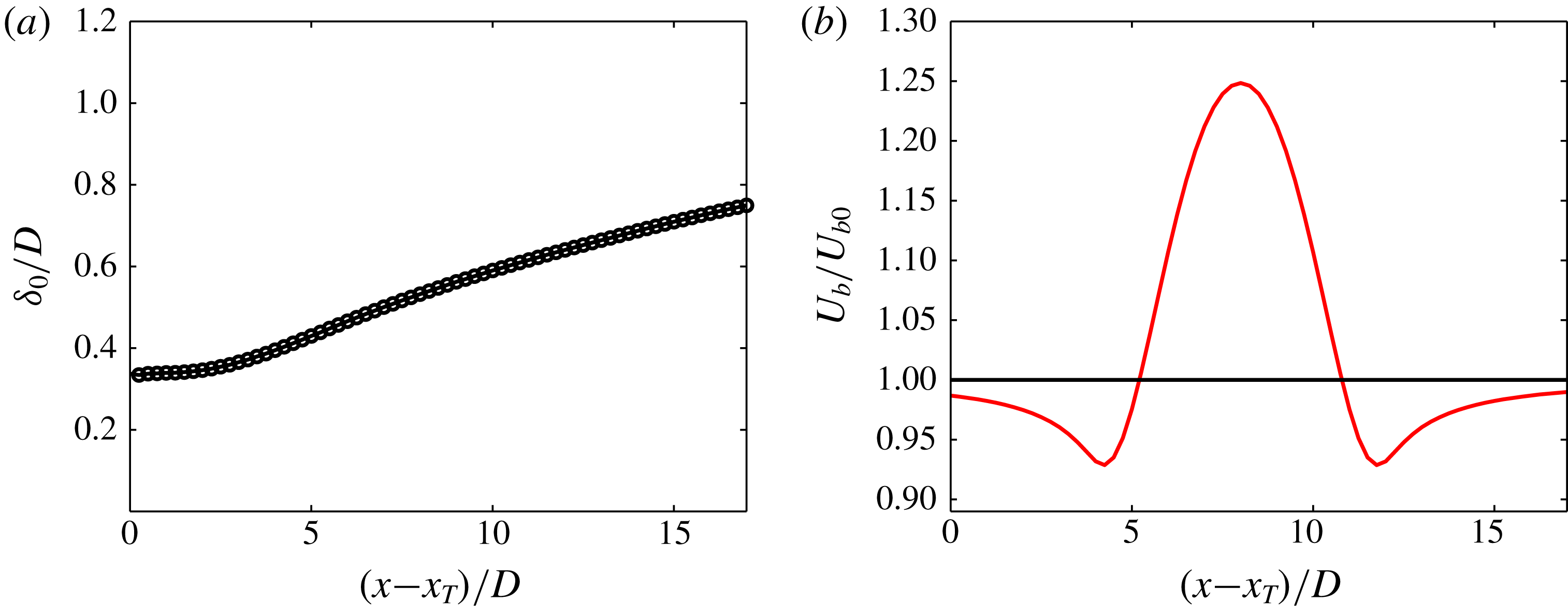
is shown in figure 13(b). The ZPG wake width
 $\unicode[STIX]{x1D6FF}_{0}(x)$
which is the wake width over the flat terrain in our case is another input which is obtained by LES and shown in figure 13(a).
The inputs of the model. (a) The wake width over flat terrain. (b)
 $U_{b}(x)$
as obtained from (2.13) (i.e.
 $U_{b}(x)=U_{nw}^{h}(x)=\overline{u}_{nw}^{U}(x,y_{h},z=Z_{h}+Hf(x/L))$
) for the hill (red line) and flat terrain (black line).
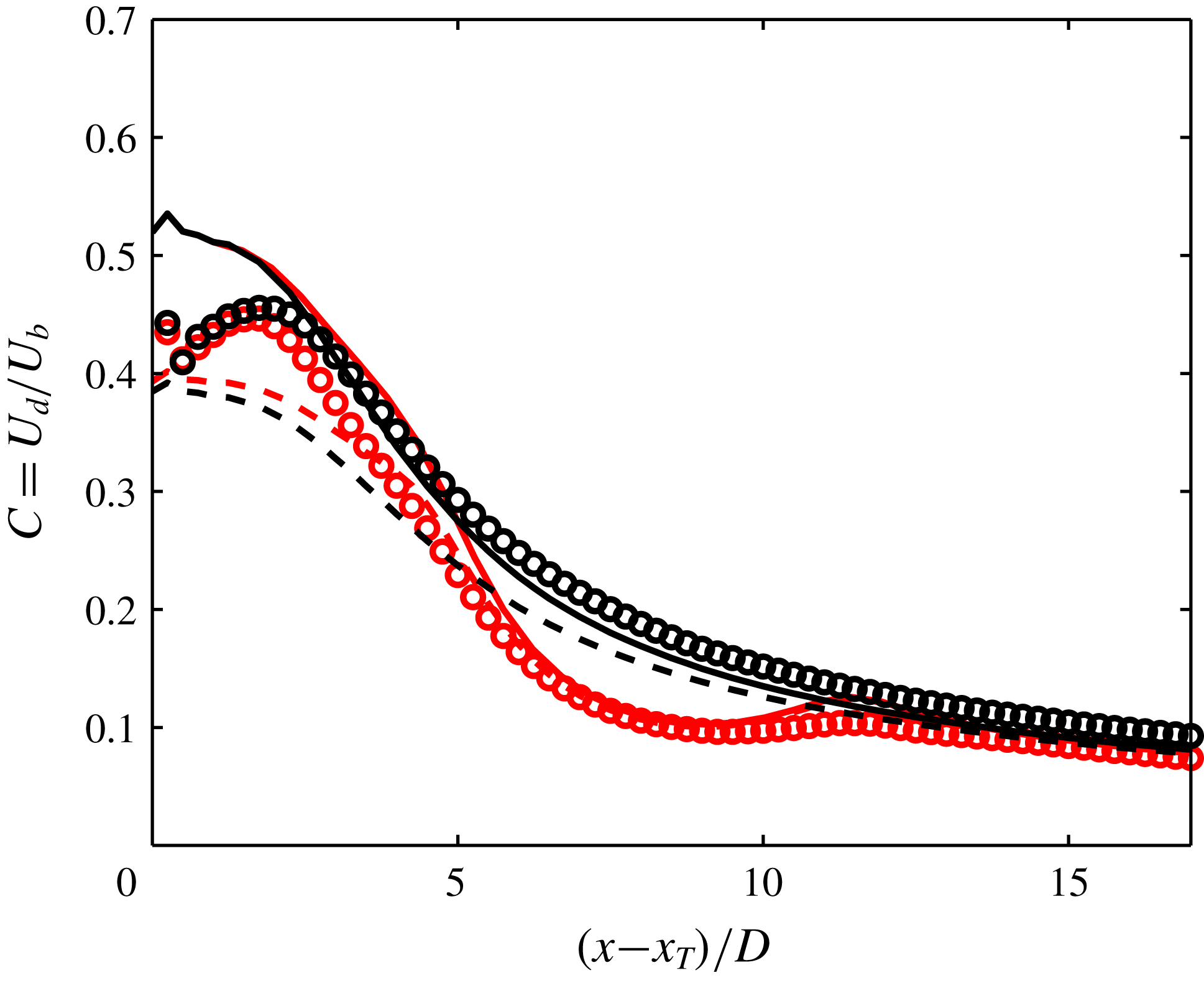
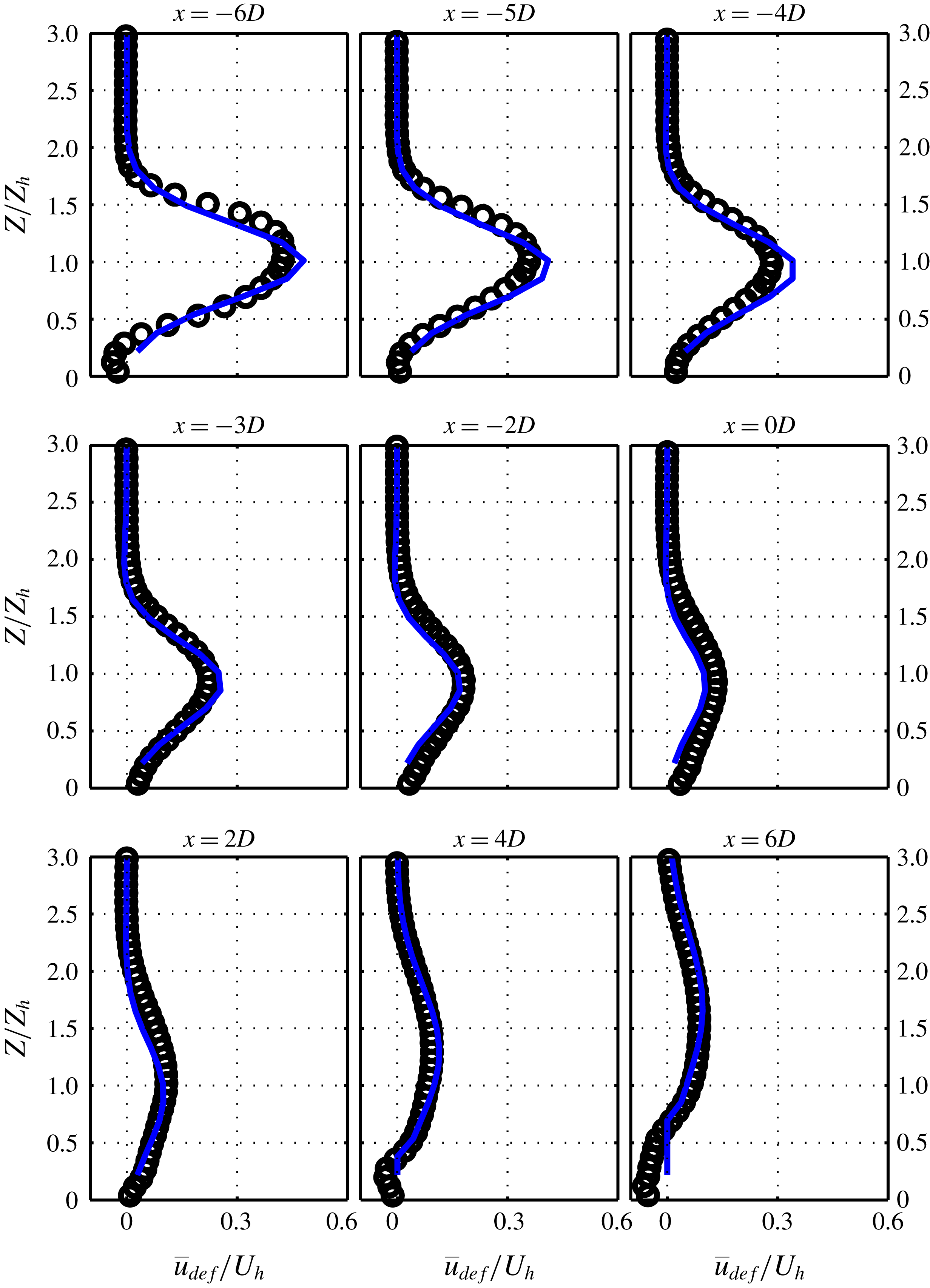
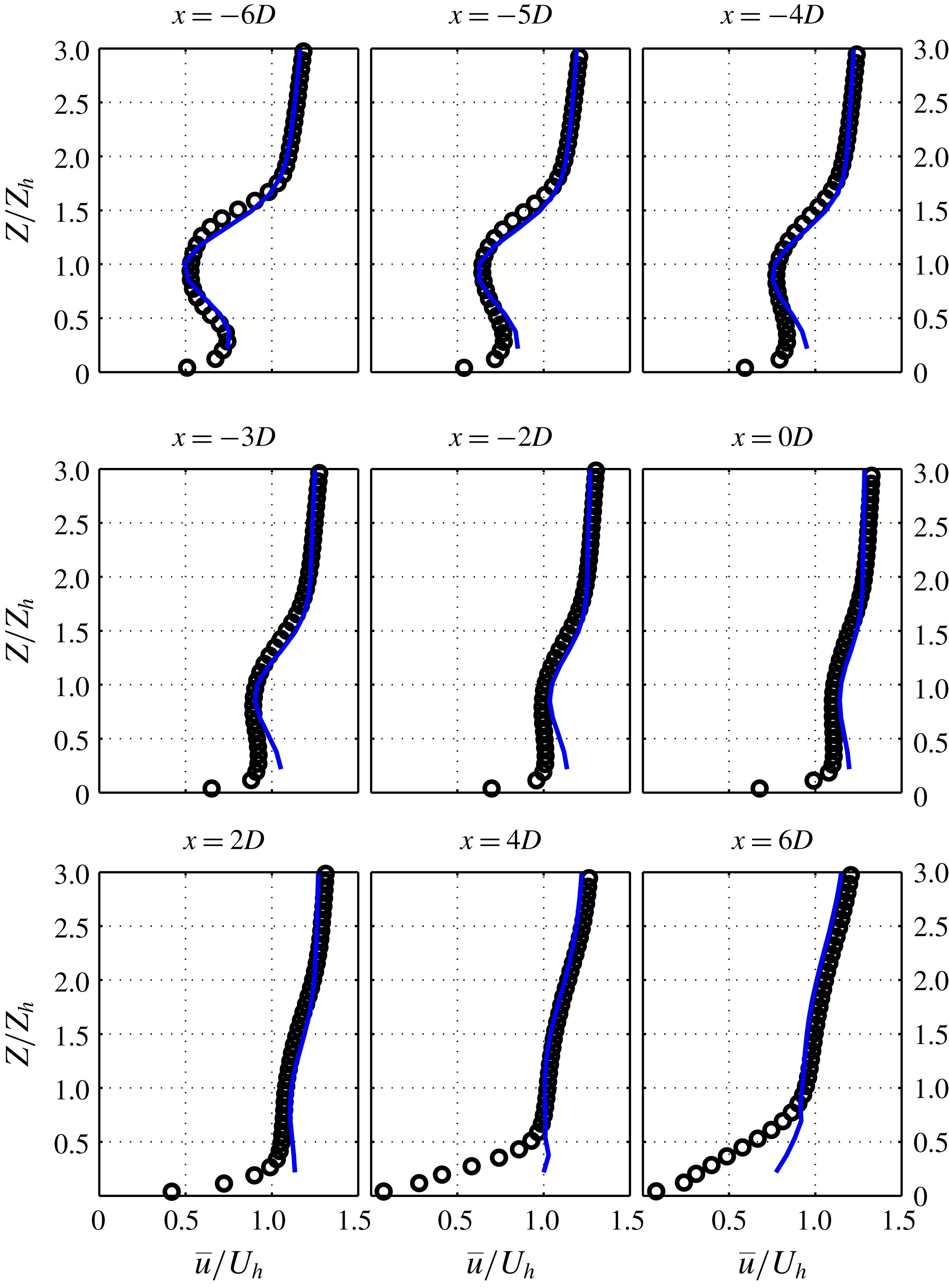
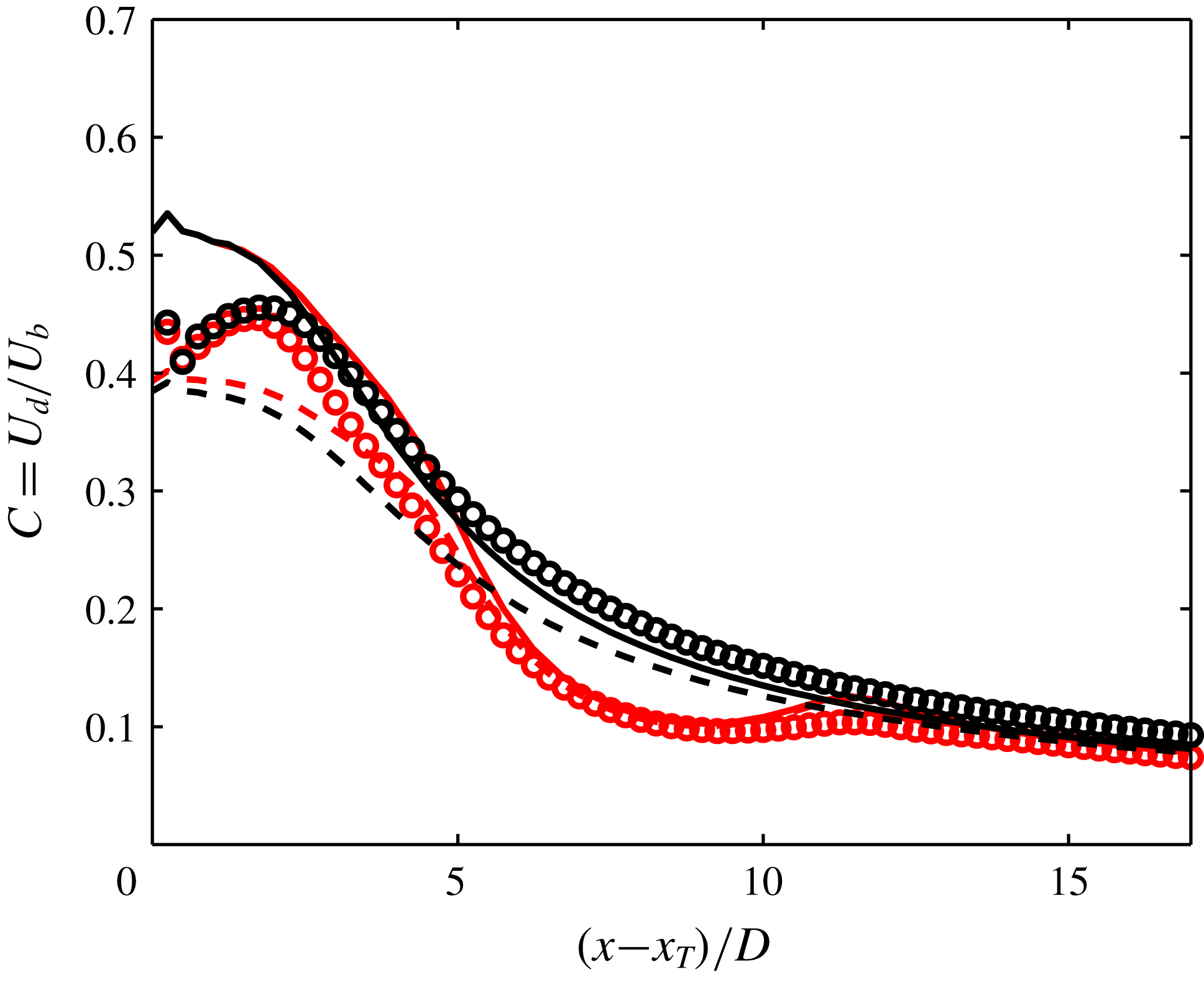
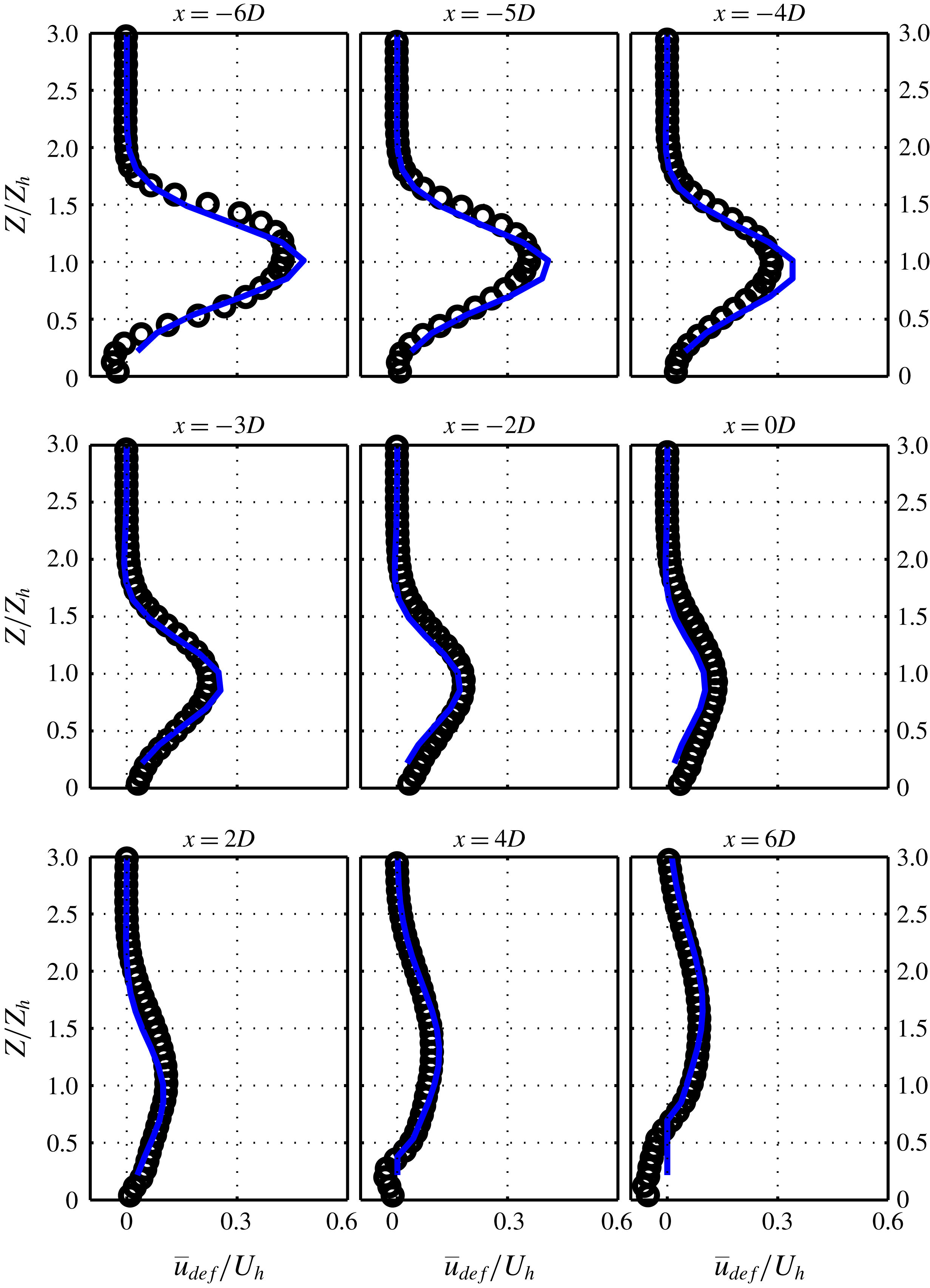
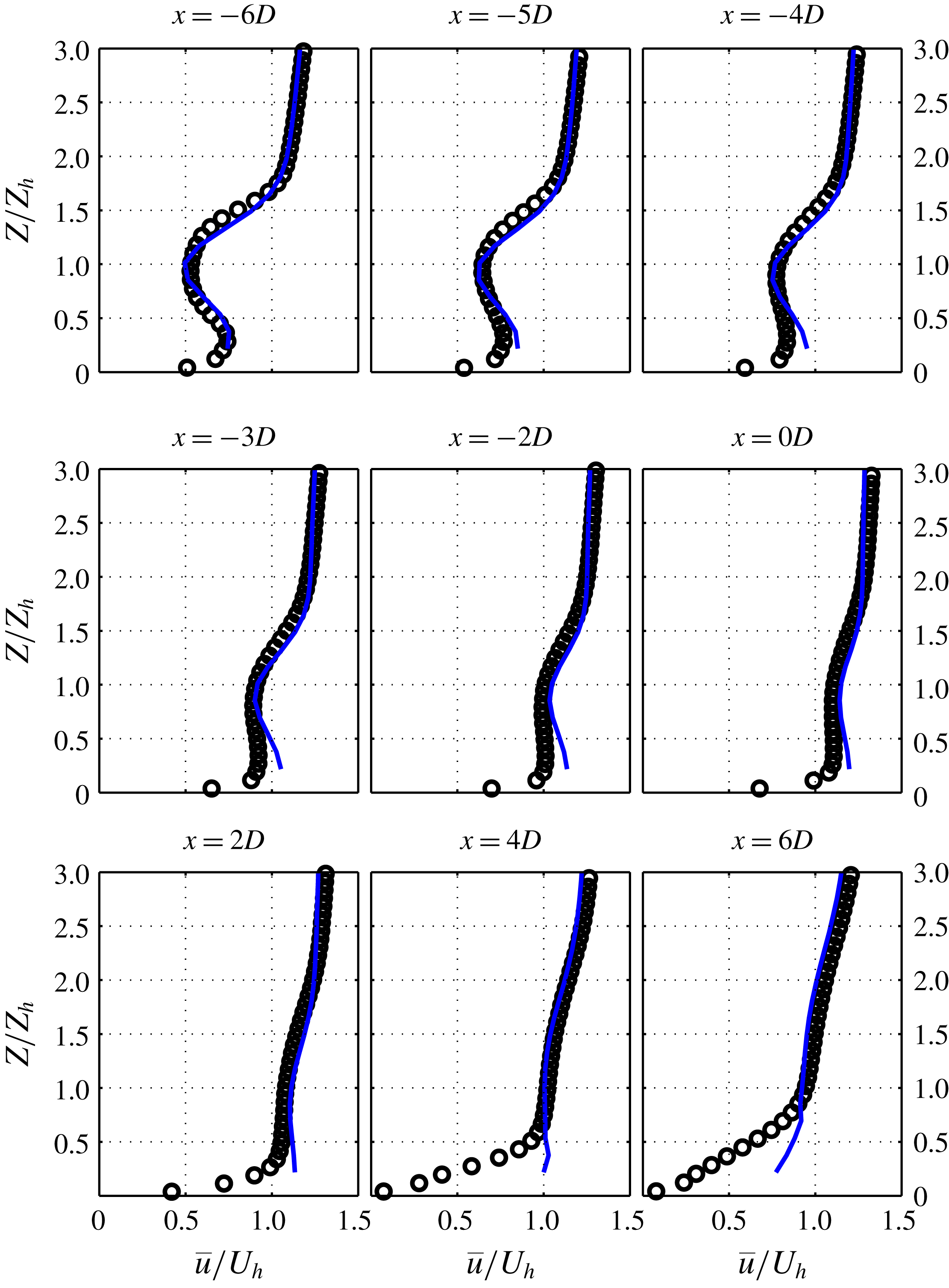
With these inputs available, we can use the model and assess its results. In figure 14, the recovery of the wake centre velocity for the flat-terrain and hill cases can be seen. The effect of pressure gradient can be seen and the model shows good capability of capturing it. Moreover, figures 15 and 16 show the velocity deficit and velocity profiles of the wake flow over the hill at different streamwise positions. It can be seen that the agreement between the analytical model and the LES results is good. We have also reproduced the streamwise velocity field in the vertical midplane of the domain in figure 17. This contour plot should be compared with the one in figure 7. It is also noteworthy that the important assumption of the linearized model, i.e. the irrotationality of the perturbation velocity field in the upper layer in § 2.3.2, was checked successfully with our LES data; however, for the sake of brevity, the results are not included here.
The wake centre trajectory can also be elicited from the already-presented framework. Up until the hilltop, equation (2.22) is used, and for the leeward side, as explained in § 4.1, a horizontal constant-elevation line is considered as an approximation for the wake centre trajectory. This is shown in figure 18. The wake centre trajectory for an escarpment (based on (4.1)) is also plotted in this figure. The agreement between the trajectories obtained from LES and the predicted trajectories is good.
Normalized velocity deficit profiles at different streamwise positions obtained from LES (black circles) and the analytical model (blue line).
Normalized mean streamwise velocity profiles at different streamwise positions obtained from LES (black circles) and the analytical model (blue line).
Contours of velocity deficit in the
 $xz$
-plane predicted by the model.
Trajectory of the wake obtained from LES (blue lines), the analytical model for the symmetric hill (red line) and the model for the escarpment (green line). For a more detailed legend, refer to the caption of figure 12.
6 A closer look into the effect of pressure gradient on the wake recovery over hills
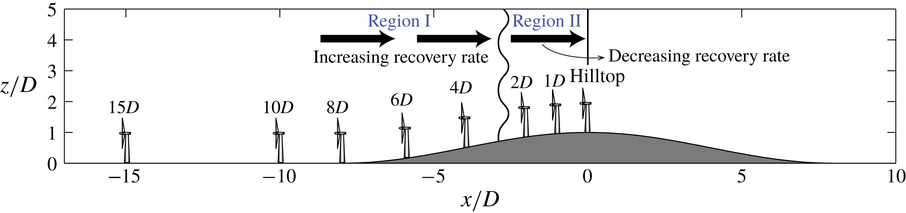
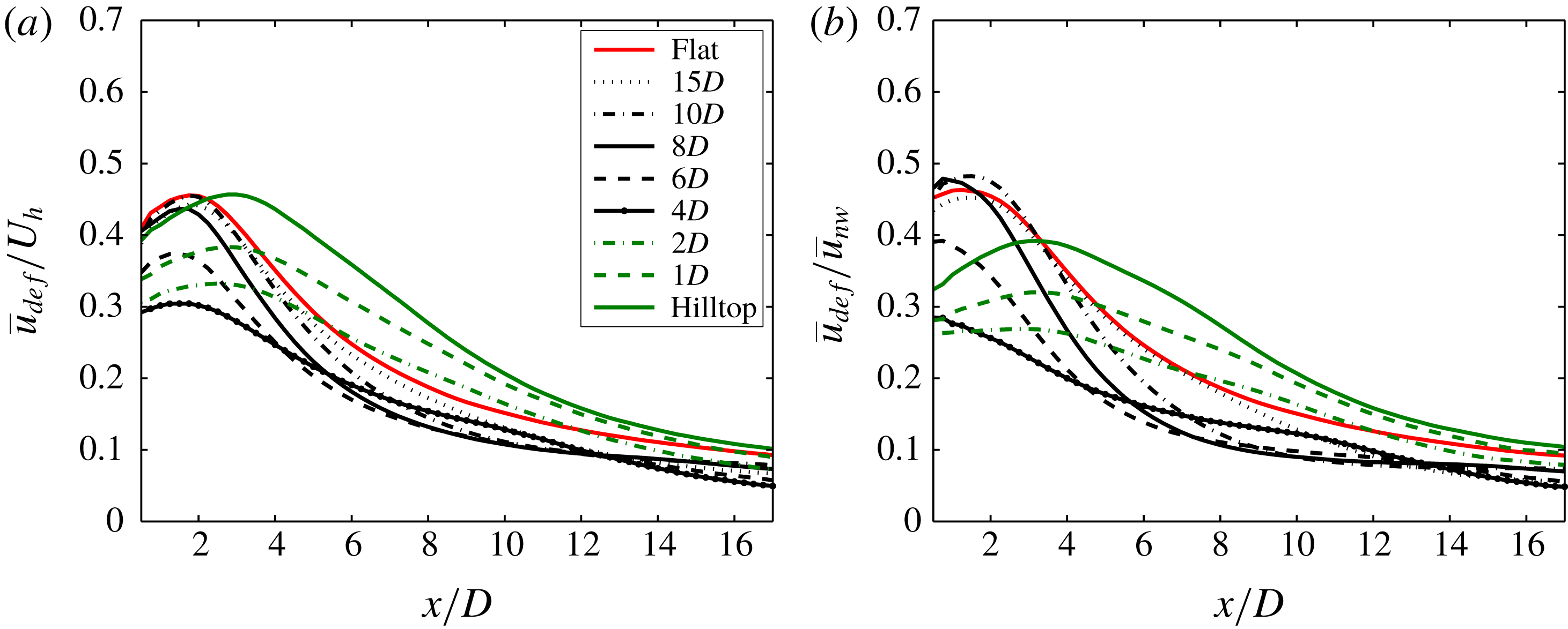
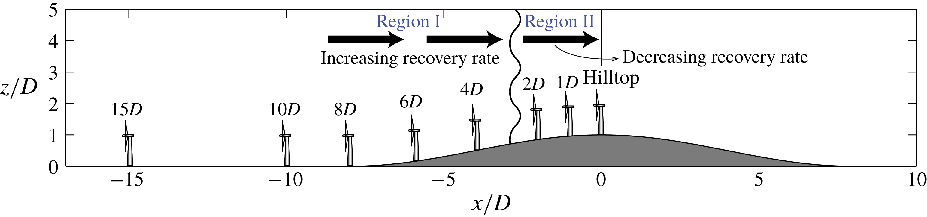
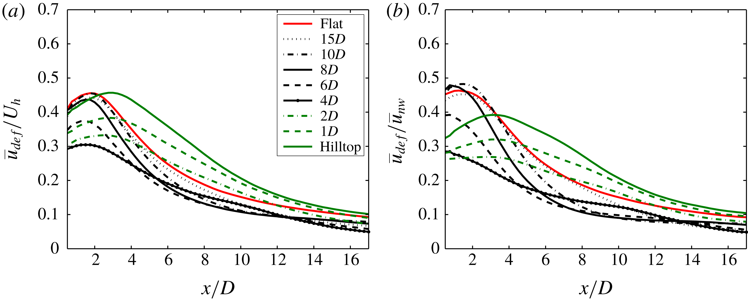
In this section, we aim to illustrate the effect of pressure gradient on wake recovery over hills more clearly, as we believe this effect is an important factor that differentiates wake flows over topography from the ones over flat terrain. To do this, we place the turbine in different upwind locations with respect to the hill and compare its recovery with the flat-terrain case. We change the position of the turbine from far upstream of the hill to the hilltop, as shown in figure 19. Figure 20 shows the recovery of the wake centre velocity for all the cases together with the flat-terrain wake. In this figure,
 $\overline{u}_{def}$
is normalized in two ways; in (a), a constant value of
 $U_{h}$
is used, and in (b), the deficit at each point is normalized by the no-wake velocity of exactly the same point. Both ways are useful. The first way is easy to interpret and use, as all of the curves are normalized with a constant value. The second way is insightful, because it takes into account the magnitude of the velocity at the position of the turbine in the no-wake case. For example, the mere fact that the velocity at the hilltop is larger than the one at the foot of the hill leads to a higher magnitude of velocity deficit for a turbine (with the same thrust coefficient) placed at the hilltop. Thus, to remove this effect from our comparison we can normalize the deficit by the local velocity in the no-wake case.
As can be seen, by moving the turbine position, the changes in the wake recovery are significant. The important observation is that, when the turbine keeps approaching the hilltop from far upstream, the recovery rate keeps increasing up until a certain point with a certain distance to the hilltop (region I in figure 19). After this point, if we move the turbine closer to the hilltop, the recovery rate keeps decreasing (region II). This is especially clear when the turbine is placed at the hilltop, where the wake recovers significantly more slowly due to the adverse pressure gradient on the leeward side of the hill (this is in agreement with what Politis et al. Reference Politis, Prospathopoulos, Cabezon, Hansen, Chaviaropoulos and Barthelmie2012 have observed). This trend is also illustrated schematically in figure 19. The above-described trend in the wake recovery rate can have implications for the turbine placement in a wind farm, i.e. depending on the position with respect to the hill, the streamwise spacing between two turbines should/can be more (e.g. in region II) or less (e.g. in region I) than the spacing between the same turbines on the flat terrain.
Schematic of different turbine placements with respect to the hill. The distance of the turbine to the hilltop is shown on top of the turbine for each placement case.
Wake centre velocity recovery for different turbine positions with respect to the hill. The legend relates to figure 19.
7 Conclusion
We have developed an analytical framework to model the behaviour of wind turbine wakes over two-dimensional hills. The model comprises two steps: first, the response of the wake evolution to the pressure gradient caused by the hill is calculated; second, the response of the wake to the streamline distortion caused by the hill is modelled. The first step was achieved by using a recently developed model by Shamsoddin & Porté-Agel (Reference Shamsoddin and Porté-Agel2018), and the second step was accomplished by performing a linearized perturbation analysis. Furthermore, we benefit from LES to obtain more detailed knowledge about the wake flow over hills. In particular, we use LES data to compare the results of the analytical model with, and also to better understand the behaviour of the wake on the leeward side of the hill. We also performed numerical experiments to better clarify the effect of the hill-induced pressure gradient on the wake recovery, by changing the position of the turbine with respect to the hill.
It was shown that the wake recovers faster on the windward side of the hill than its leeward side, due to the mainly favourable pressure gradient on the windward side and the adverse one on the leeward side. The trajectory of the wake was found to closely follow the terrain on the windward side of a hill with the same height as the turbine hub height and moderate slope. However, on the leeward side, the trajectory showed little dependence on the hill profile and mainly maintained a constant elevation. The trajectory of the wake on the leeward side was also studied for the limiting case of an escarpment, and it was shown that an IBL forms on the plateau which leads to an upward displacement of the wake centre. This displacement was also quantified by using models available in the literature.
There is much room for more investigations on this topic. First of all, systematic parametric studies of the turbine–hill systems are needed. In fact, several key geometrical features are involved in this problem (e.g. hill height to hub-height ratio, hill slope, position of the turbine with respect to the hill), whose effects should be systematically studied. The present analysis can be extended to three-dimensional hills. Such hills are likely to have special effects on the wake behaviour which differentiate them from 2-D hills. Finally, there is a shortage of high-resolution wind tunnel measurements of wakes over hills, which makes new experimental research on this subject highly valuable.
Acknowledgements
This research was supported by the Swiss Federal Office of Energy (Grant SI/501337-01) and the Swiss National Science Foundation (grant 200021_172538). In addition, this project is carried out within the framework of the Swiss Centre for Competence in Energy Research on the Future Swiss Electrical Infrastructure (SCCER-FURIES) with the financial support of the Swiss Innovation Agency (Innosuisse – SCCER program) (contract number: 1155002544). Computing resources were provided by the Swiss National Supercomputing Centre (CSCS) under Project ID s706.
Appendix A. Summary of the model
Herein, we provide a summary of the model, to facilitate its application by the reader. For this purpose, we review and clarify the inputs to the model, its outputs, the procedure to calculate the outputs and finally the nomenclature of the key variables.
A.1 Inputs to the model
The inputs to the model are the following:
(1) The inflow mean streamwise velocity profile on flat terrain
 $U_{nw}(z)$
. For the case of a typical logarithmic profile, this reduces to determining the friction velocity
$u_{\ast }$
and the surface roughness length
$z_{0}$
.
(2) The hill geometry, or in other words the terrain surface equation,
$z_{s}=Hf(x/L)$
, where
$H$
is the height at the hilltop,
$L$
is the half-length of the hill,
$f(x/L)\leqslant 1$
and
$f(0)=1$
.(3) The turbine characteristics (geometrical and mechanical) including: turbine hub height
$Z_{h}$
, turbine diameter
$D$
, position of the turbine with respect to the hilltop
$x_{T}$
and thrust coefficient of the turbine
$C_{T}$
.(4) The wake width of the turbine on flat terrain (i.e. in ZPG case)
$\unicode[STIX]{x1D6FF}_{0}(x)$
.


A.2 Outputs of the model
The outputs of the model are the following:
(1) The recovery of the wake maximum velocity deficit
$C(x)$
.(2) The velocity deficit profiles over the hill
$\overline{u}_{def}(x,y,Z)$
.(3) The velocity profiles over the hill
$\overline{u}_{w}^{UM}(x,y,Z)$
.(4) The wake trajectory
$Z_{c}(x)$
.


A.3 Procedure to obtain the desired outputs
The procedure to obtain the above-mentioned outputs given the above-mentioned inputs is the following.
The model has two steps (see figure 1). Moreover, a special treatment is proposed for the behaviour of the wake on the leeward side of the hill.
(I) The first step of the model accounts for the effect of the hill-induced pressure gradient on the wake recovery (see § 2.2):
(1) First, we need the velocity of the flow under pressure gradient but without the wake, that is,
$U_{b}(x)$
. For this purpose, we use
$U_{b}=U_{nw}^{h}(x)$
, where
$U_{nw}^{h}(x)$
is obtained from the no-wake case of (2.13) (this is the same as the solution of Jackson & Hunt Reference Jackson and Hunt1975). In other words,
$U_{nw}^{h}(x)=\overline{u}_{nw}^{U}(x,y_{h},z=Z_{h}+Hf(x/L))$
, i.e. the velocity at a distance equal to the hub height (
$Z_{h}$
) from the ground in the case without the wind turbine. Note that
$\overline{u}_{nw}^{U}$
is a function of
$z$
and not
$Z$
, which is why we use
$z=Z_{h}+Hf(x/L)$
to get the locus of the points whose distance from the ground is
$Z_{h}$
. Notice also that to use (2.13), we first need to get
$\unicode[STIX]{x0394}u^{U}$
from (2.12). In this step, we have used inputs (1) and (2) in § A.1.(2) We obtain
$C_{0}(x)$
and
$\unicode[STIX]{x1D706}_{0}(x)$
from (2.4) and (2.5), respectively. Inputs (3) and (4) are used in this step.(3) Now, we can first obtain
$C(x)$
from (2.2) and then
$\unicode[STIX]{x1D6FF}(x)$
from (2.6).(4) At this stage, the wake velocity function
$\overline{u}(x,r)$
in the imposed pressure gradient is given by (2.1).
(II) The second step of the model accounts for the effect of the hill-induced streamline distortion (see 2.3):
(1) For both no-wake and wake cases, we use equation (2.16) to obtain
$\unicode[STIX]{x0394}u_{t}$
. For the no-wake case, we call it
$\unicode[STIX]{x0394}u_{t,nw}^{M}$
, and for the wake case, we call it
$\unicode[STIX]{x0394}u_{t,w}^{M}$
. Note that to be able to use (2.16), we also need to get
$B(x,y)$
from (2.17), and
$U(x,y,z)$
from (2.18).(2) Now, we are able to calculate the wake velocity deficit over the hill
$\overline{u}_{def}(x,y,Z)$
from (2.20). To do this, we need to first obtain
$\overline{u}_{nw}^{M}$
and
$\overline{u}_{w}^{M}$
from (2.19).(3) Next, we obtain the wake flow velocity distribution
$\overline{u}_{w}^{UM}(x,y,Z)$
from (2.21). To do this, we need to first calculate
$\overline{u}_{nw}^{U}(x,y,Z+Hf(x/L))$
from (2.13).(4) Finally, we obtain the wake trajectory
$Z_{c}(x)$
from (2.22).
(III) The wake on the leeward side of the hill is modelled as follows (see § 4).
(1) Trajectory correction:
(i) for hills we have
$Z_{c}(x>x_{ht})=Z_{c}(x=x_{ht})=Z_{c}^{ht}$
.(ii) for escarpments we have
$Z_{c}(x>x_{ht})=Z_{c}^{ht}+\unicode[STIX]{x0394}Z_{c}(x)$
, where
$\unicode[STIX]{x0394}Z_{c}(x)$
is the solution of (4.1) after replacing
$\unicode[STIX]{x0394}Z_{p}$
by
$\unicode[STIX]{x0394}Z_{c}$
.
(2) To reflect this trajectory modification in the velocity profiles on the leeward side, we can simply centre the calculated velocity deficit (i.e. 2.20) around this trajectory.














A.4 Nomenclature of key variables
The following table presents a nomenclature of the key variables used in this paper (especially those used in the analytical modelling).
Summary of the key variables
- Variable
Definition
-
$U_{b}(x)$
Velocity of the flow under pressure gradient in the no-wake case, which is used only in the first step of the model (i.e. the effect of the hill-induced pressure gradient on the wake recovery).
-
$C(x)$
A function determining the maximum velocity deficit at each
$x$
-position. It is equal to the ratio of the maximum velocity deficit (
$\text{max}(U_{b}(x)-\overline{u}(x,r))$
) to the local no-wake flow velocity, i.e.
$U_{b}(x)$
.-
$\unicode[STIX]{x1D6FF}(x)$
Wake width.
-
$\unicode[STIX]{x1D6FF}_{0}(x)$
Wake width for the zero-pressure-gradient case.
-
$U_{nw}^{h}(x)$
The no-wake flow velocity over the hill at hub height (
$Z_{h}$
) from the ground. This is used to obtain
$U_{b}(x)$
.-
$z_{s}(x)$
The surface equation of the hill. This is taken equal to:
$z_{s}=Hf(x/L)$
.-
$z$
Elevation from a horizontal fixed level (see figure 3).
-
$Z$
Height above the ground.
$Z=z-z_{s}$
(see figure 3).-
$U$
The base flow mean streamwise velocity, i.e. the velocity when the hill is not present (over flat terrain). The base flow velocity can be either in the no-wake case (
$U_{nw}$
) or in the wake case (
$U_{w}$
).-
$\overline{u}$
Total flow velocity, including the perturbation induced by the hill.
-
$\unicode[STIX]{x0394}u$
The perturbation velocity caused by the hill, which should be added to
$U$
to result in
$\overline{u}$
, i.e.
$\overline{u}=U+\unicode[STIX]{x0394}u$
.-
$\unicode[STIX]{x0394}v$
,
$\unicode[STIX]{x0394}w$
Similar to above.
-
$\overline{u}_{def}$
Velocity deficit, i.e.
$\overline{u}_{def}=\overline{u}_{nw}-\overline{u}_{w}$
.-
$\overline{u}_{w}^{UM}$
The modelled total velocity of the flow when both the hill and the turbine are present, which is the result of the addition of the total no-wake velocity computed in the upper layer and the velocity deficit computed in the middle layer. That is,
$\overline{u}_{w}^{UM}=\overline{u}_{nw}^{U}-\overline{u}_{def}$
(see equation 2.21).-
$Z_{c}$
Height of the wake centre above the ground.
-
$z_{c}$
Elevation of the wake centre from a horizontal fixed level.
-
$Z_{c}^{ht}$
(or
$z_{c}^{ht}$
)
Height from the ground (elevation from a horizontal fixed level) of the wake centre at the hilltop.
-
$h_{m}$
Height of the middle layer.
-
$z_{o}$
Surface roughness length.
-
$x_{T}$
Streamwise position of the turbine.
-
$Z_{h}$
Hub height of the turbine.
-
$D$
Rotor diameter of the turbine.
-
$H$
Height of the hill.
-
$L$
Half-length of the hill.





Subscript
-
$0$
Shows a variable in the zero-pressure-gradient case.
-
$t$
Shows a variable in the terrain-following coordinates (see § 2.3.1).
-
$nw$
Shows a variable in the no-wake case, i.e. the case in which the turbine is not present.
-
$w$
Shows a variable in the wake case, i.e. the case in which the turbine is present.
- def
Shows a velocity deficit, i.e. the difference between velocities of the wake and no-wake cases at the same position in space.
-
$c$
Shows a variable related to the wake centre.


Superscript
-
$\overline{\,\,\,}$
Shows a mean quantity.
-
$U$
Shows a variable in the upper layer.
-
$M$
Shows a variable in the middle layer.
-
$ht$
Shows a variable at the hilltop.