2.1 Added mass in homogeneous and stratified fluids

When an object moves in an ideal fluid, it has to move the fluid around in order to pass through. As the fluid has a given density, a higher force is necessary to displace the object in the fluid than in the vacuum. Indeed, as both the object and the surrounding fluid have to be accelerated, the necessary force is equal to the acceleration of the object multiplied by the mass of the object and another mass $m_{A}$ , due to the fluid (Lamb Reference Lamb1932). This mass is called the added mass and depends on the shape of the object in the fluid. It is generally described using a tensor. In naval architecture, the added mass plays an important role because it can easily be of the same order of magnitude as the total mass of a ship or a submarine (Newman Reference Newman1977; Brennen Reference Brennen1982).

Figure 1.

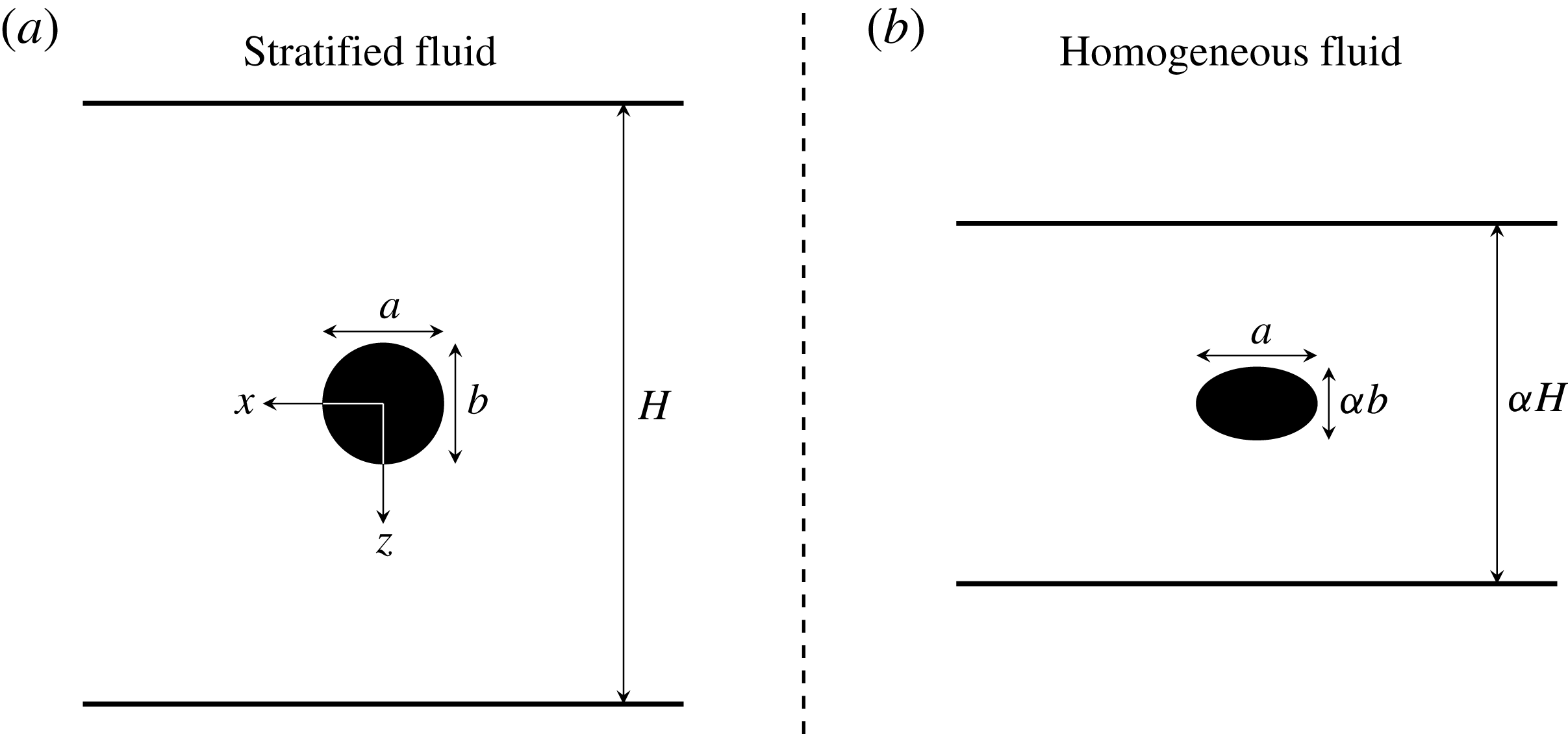
Geometries of the original and fictitious problems. (a) Two-dimensional object oscillating horizontally at the non-dimensional frequency $\unicode[STIX]{x1D6FA}$ in a linearly stratified fluid of depth $H$ . The horizontal and vertical sizes of the object are $a$ and $b$ , respectively. (b) Fictitious body oscillating horizontally in a homogeneous fluid after an affine transformation of the object in (a). The transformation changes the vertical scales by a factor $\unicode[STIX]{x1D6FC}=(\unicode[STIX]{x1D6FA}^{2}-1)^{1/2}/\unicode[STIX]{x1D6FA}$ , for $\unicode[STIX]{x1D6FA}>1$ . The horizontal and vertical sizes of the fictitious object are $a$ and $b_{\ast }=\unicode[STIX]{x1D6FC}b$ , respectively. The fluid has a depth of $\unicode[STIX]{x1D6FC}H$ .

Added mass can be used to investigate the tidal conversion in the oceans (Voisin et al. Reference Voisin, Ermanyuk and Flor2011), which are continuously stratified in density. In such a fluid, internal waves can propagate using buoyancy as a restoring force. One defines the buoyancy frequency $N=[(g/\bar{\unicode[STIX]{x1D70C}})(\text{d}\unicode[STIX]{x1D70C}/\text{d}z)]^{1/2}$ , where $\unicode[STIX]{x1D70C}(z)$ is the density distribution over vertical coordinate  $z$ , $\bar{\unicode[STIX]{x1D70C}}$ a reference value and $g$ the gravity acceleration. Note that, here, the vertical axis  $z$ points downwards, as shown in figure 1. The dispersion relation of internal waves is $\unicode[STIX]{x1D714}/N=\pm \sin \unicode[STIX]{x1D703}$ where $\unicode[STIX]{x1D703}$ is the angle between the direction of propagation of the wave and the horizontal, and $\unicode[STIX]{x1D714}$ the frequency of the wave. In the ocean, internal waves are created thanks to the tidal oscillations of the fluid upon the topographies. This can also be viewed as topographies oscillating in a stratified fluid. The two problems are totally equivalent for small amplitude oscillations.

Let us consider an object oscillating horizontally in a stratified fluid. With the dispersion relation, internal waves can only be emitted if the body oscillates at a frequency  $\unicode[STIX]{x1D714}$ smaller than $N$ . This leads to two different behaviours of the body depending on the frequency of the oscillations. If $\unicode[STIX]{x1D714}>N$ , no wave can be emitted, and the added mass is a real-valued function of $\unicode[STIX]{x1D714}$ . But if $\unicode[STIX]{x1D714}<N$ , waves are emitted by the body and the added mass becomes a complex-valued function of $\unicode[STIX]{x1D714}$ . For unidirectional rectilinear oscillations of a body having three planes of symmetry, the added mass can be decomposed in two parts (Lai & Lee Reference Lai and Lee1981; Ermanyuk Reference Ermanyuk2002)

where the real part $\unicode[STIX]{x1D707}$ corresponds physically to the force component oscillating in phase with the acceleration of the body (inertial force), and the imaginary part $\unicode[STIX]{x1D706}_{w}(\unicode[STIX]{x1D714})/\unicode[STIX]{x1D714}$ corresponds to the force component oscillating in phase with the velocity of the body (damping force). $\unicode[STIX]{x1D707}$ is therefore called the inertial mass while $\unicode[STIX]{x1D706}_{w}$ is the wave damping rate, proportional to the radiated wave power as follows

$A$ being the amplitude of oscillations. The power is directly related to the tidal conversion, with $U=A\unicode[STIX]{x1D714}$ , the amplitude of tidal velocity. Note that we assume an ideal fluid. In a real fluid, as in experiments, the motion of the object is affected by viscosity. Thus, in a uniformly stratified fluid when $\unicode[STIX]{x1D714}>N$ , there is only a viscous damping while, when $\unicode[STIX]{x1D714}<N$ , the damping is due to the combined effects of wave radiation and viscosity. Note that, in the latter case, the largest part of the energy dissipation is associated with the wave emission (see for example Ermanyuk (Reference Ermanyuk2000, Reference Ermanyuk2002)).

2.2 Affine similitude in a linearly stratified fluid

Let us consider a two-dimensional object submerged at depth $H/2$ in a channel of full depth $H$ filled with an ideal uniformly stratified fluid, as sketched in figure 1(a). We assume that the horizontal extent of the channel is infinite. The upper and lower boundaries of the channel are assumed to be rigid. A Cartesian coordinate system is introduced with the $x$ -axis located at mid-depth of fluid and pointing to the left and $z$ -axis pointing downwards. The $y$ -axis is horizontal and perpendicular to the $x$ -axis. The horizontal and vertical sizes of the object are denoted $a$ and $b$ , respectively. One defines the aspect ratio of the body $p=b/a$ and the non-dimensional vertical size of the body $q=b/H$ . We restrict our consideration to the case of horizontal harmonic oscillations of the object with frequency $\unicode[STIX]{x1D714}$ and amplitude $A$ . The non-dimensional frequency is introduced as $\unicode[STIX]{x1D6FA}=\unicode[STIX]{x1D714}/N$ . Note that on figure 1(a), the body is a circular cylinder but the theoretical preliminaries of this section are also valid for any other shapes. Below we consider experimentally the cases of cylinders with cross-sections being a disk, a line and a double flat top. In the oceanographic context, these geometries correspond to the semi-circular, knife-edge and flat-top ridges.

Let us consider first the problem where $\unicode[STIX]{x1D6FA}>1$ , i.e. where the added mass is a real quantity. The added mass coefficient $K$ of a body undergoing horizontal oscillations at the dimensionless frequency $\unicode[STIX]{x1D6FA}$ in a uniformly stratified fluid are known (Ermanyuk Reference Ermanyuk2002) to be related with the added mass coefficient $K_{\ast }$ of a fictitious affinely similar body oscillating in a homogeneous fluid

Here, the added mass coefficients are defined as $K=m_{A}/\unicode[STIX]{x1D70C}_{0}S$ and $K_{\ast }=m_{A\ast }/\unicode[STIX]{x1D70C}_{0}S_{\ast }$ , where $\unicode[STIX]{x1D70C}_{0}$ is the reference density at the depth corresponding to the centre of the body, $m_{A}$ and $m_{A\ast }$ are the added masses per unit length, $S$ and $S_{\ast }$ are the cross-sections of the original and fictitious bodies, respectively. The fictitious problem is obtained by compressing the original body and channel in the vertical direction $\unicode[STIX]{x1D6FC}$ times, where $\unicode[STIX]{x1D6FC}=(\unicode[STIX]{x1D6FA}^{2}-1)^{1/2}/\unicode[STIX]{x1D6FA}$ . This is shown in figure 1(b) where the fictitious body is an ellipse of major axis $a$ and minor axis $b_{\ast }=\unicode[STIX]{x1D6FC}b$ and where the fictitious channel has a height  $\unicode[STIX]{x1D6FC}H$ . Consequently, the cross-section area $S=\unicode[STIX]{x03C0}ab/4$ of the original body is transformed in $S_{\ast }=\unicode[STIX]{x03C0}ab_{\ast }/4=\unicode[STIX]{x1D6FC}S$ for the fictitious body. Note that as the fictitious body oscillates in a homogeneous fluid, its added mass coefficient $K_{\ast }$ is independent of the frequency of oscillations. Therefore, the dependence on $\unicode[STIX]{x1D6FA}$ for $K$ only comes from the dependence of $K_{\ast }$ on the compression coefficient $\unicode[STIX]{x1D6FC}$ . Moreover, when $\unicode[STIX]{x1D6FA}$ becomes much greater than $1$ , $\unicode[STIX]{x1D6FC}$ tends to $1$ . Thus, the original and fictitious problem geometries are the same for high oscillation frequencies. The added mass coefficient in the original problem for high frequency is supposed to tend to the one measured in the homogeneous case, with the same geometry.

In many problems, it is more convenient to normalize the added mass of the oscillating cylinder by the added mass of a flat plate of height $b$ so that $k=m_{A}/(\unicode[STIX]{x1D70C}_{0}\unicode[STIX]{x03C0}b^{2}/4)$ and $k_{\ast }=m_{A\ast }/(\unicode[STIX]{x1D70C}_{0}\unicode[STIX]{x03C0}b_{\ast }^{2}/4)$ . This normalization is particularly suitable in geophysical fluid dynamics in view of the scaling used for the tidal conversion (Llewellyn Smith & Young Reference Llewelyn Smith and Young2003). Obviously, with such a normalization, equation (2.3) should be replaced by

Equation (2.3) has been obtained by Ermanyuk (Reference Ermanyuk2002) by considering the integrals of pressure over the body surface and the control surface surrounding the body, and applying the Gauss theorem to the fluid volume located between these surfaces, in spirit of Newman (Reference Newman1977). The control surface can be a material surface that undergoes the same affine transformation as the body surface. In this case, equation (2.3) remains valid since the conversion factors relating surface integrals over original and fictitious bodies, as well as over original and transformed control surfaces, are the same. However, to extend the solution to the case $\unicode[STIX]{x1D6FA}<1$ , one should keep in mind that the control surface cannot be a closed one. There must be a possibility for radiation of internal wave energy.

Now we consider a body belonging to a certain family of shapes and oscillating in a homogeneous fluid between two horizontal parallel rigid planes. Let us suppose that we know the function, representing the dependence of the added mass coefficients on non-dimensional geometrical parameters $p=b/a$ and $q=b/H$ for this family of bodies

Note that $q=b/H$ does not change under affine transformation. Then, for $\unicode[STIX]{x1D6FA}>1$ , the added mass coefficient of a body in a uniformly stratified fluid at certain given values of $p$ and $q$ can be found as follows

As discussed in Ermanyuk (Reference Ermanyuk2002) in the context of Hurley (Reference Hurley1997), $K(\unicode[STIX]{x1D6FA})$ and $k(\unicode[STIX]{x1D6FA})$ at $\unicode[STIX]{x1D6FA}<1$ can be obtained by the analytic continuation in frequency. This can be done if the radiation condition formulated in the causal sense does hold true, i.e. the internal waves are radiated from the source to infinity and never return. For $\unicode[STIX]{x1D6FA}<1$ , the analytic continuation for $\unicode[STIX]{x1D6FC}$ is $\text{i}\unicode[STIX]{x1D702}$ , where $\unicode[STIX]{x1D702}=(1-\unicode[STIX]{x1D6FA}^{2})^{1/2}/\unicode[STIX]{x1D6FA}$ is the real-value parameter. Accordingly, equation (2.6) becomes

Thus, knowing the added mass coefficient for a family of bodies in a homogeneous fluid, one can deduce the added mass coefficient of related bodies in a linearly stratified fluid as a function of the frequency. This can be useful because added mass in a homogeneous fluid is well studied (Brennen Reference Brennen1982; Korotkin Reference Korotkin2010) while the added mass in a stratified fluid has been investigated only recently.

When $\unicode[STIX]{x1D6FA}<1$ , the added mass is complex valued, as defined by (2.1). One can introduce the inertial coefficient

and the wave damping coefficient

Using (2.2), the dimensionless form for the radiated wave power is defined as

Note that in the case of an ideal and homogeneous fluid without free surface, one can define only the inertial coefficient $C^{\unicode[STIX]{x1D707}}$ , the damping being identically zero.

In the case of a fluid of infinite extent, equations (2.6) and (2.7) can be used to re-derive the formulas for hydrodynamic loads acting on an elliptic cylinder (Hurley Reference Hurley1997), and a vertically oscillating spheroid (Lai & Lee Reference Lai and Lee1981). Solutions for horizontally oscillating spheroids (Ermanyuk Reference Ermanyuk2002) and squares (Ermanyuk & Gavrilov Reference Ermanyuk and Gavrilov2002b ) can also be obtained. However, there are only few analytical solutions for the added mass of bodies oscillating in ideal homogeneous fluid of finite depth. The known results are limited to the cases of the vertical flat plate (Lockwood-Taylor Reference Lockwood-Taylor1930), the elliptic cylinder (Clarke Reference Clarke2001) and the rectangle (Gurevich Reference Gurevich1940; Newman Reference Newman1969).

Figure 2.

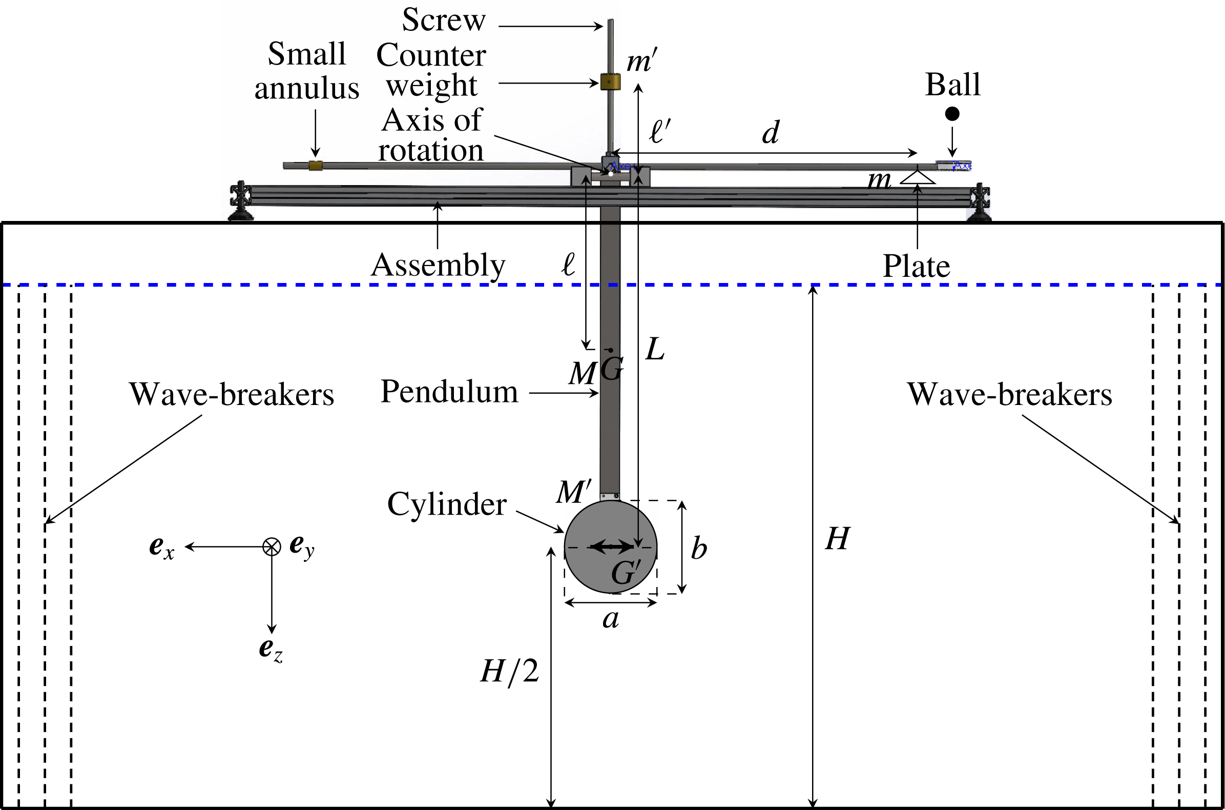
Schema of the pendulum set-up viewed from the side: arrows show the different elements of the set-up, relevant lengths are labelled and coordinates are shown. The surface of the water is the horizontal dashed blue line. The body is moving horizontally along the $x$ -axis, as depicted by the thick arrows in the centre of the body.

3.1 Experimental set-up

The experimental set-up is sketched in figure 2. It is very similar to the one described by Ermanyuk (Reference Ermanyuk2000, Reference Ermanyuk2002) and by Ermanyuk & Gavrilov (Reference Ermanyuk and Gavrilov2002a , Reference Ermanyuk and Gavrilov2003). The pendulum has a cross shape, with a massive cylinder attached at the lower end. The cylinder has a centre of gravity $G^{\prime }$ and a mass $M^{\prime }$ and is invariant in the $y$ -direction. It can have different cross-sectional shapes, a disk as in figure 2 or other shapes (see table 1). The cross-section has a horizontal (respectively vertical) length scale denoted $a$ (respectively $b$ ). The vertical arm opposite to the cylinder is a screw where two different counter weights of mass $m^{\prime }=167$  g and $m^{\prime }=704$  g can be placed. Changing the position of the counter weights with respect to the axis of rotation allows us to tune the characteristic frequency of the pendulum, defined as $\unicode[STIX]{x1D714}_{c}$ . The purpose of having two different counter weights is to be able to cover a large range of frequencies for all the shapes studied in this article. The pendulum has also two long horizontal arms. At the end of the right one, there is a small horizontal circle, covered by a tensioned rubber membrane. A ball, initially hold by an electric magnet, can be dropped on the membrane to excite the pendulum. As the period of the oscillations of the pendulum is of several seconds, if the membrane is sufficiently tight, the excitation of the pendulum is very close to an instantaneous impulse. Attached to the right arm, one also has a small plate which can contain a mass $m$ for the calibration procedure explained further, in § 3.2. On the left horizontal arm, there is a small annulus which can be displaced horizontally to adjust very precisely the horizontality of the pendulum before the beginning of each experiment. The centre of mass of the pendulum with the cylinder but without the counter weight is noted $G$ , its mass $M$ and its moment of inertia is defined as $J$ . Note that the mass of the pendulum alone, without the cylinder and the counter weight is $889$  g. All the relevant distances are defined in figure 2, with respect to the rotation axis. This axis is shown by a white spot in figure 2. $L$ and $\ell$ are given in table 1 for each cylinder. $d$ is equal to $40$  cm while $\ell ^{\prime }$ varies in the range $[5.1{-}21]$  cm. The different masses are also shown in figure 2. The coordinates are defined in figure 2, with the origin of the coordinate system taken at the centre of mass of the cylinder, $G^{\prime }$ .

Table 1.

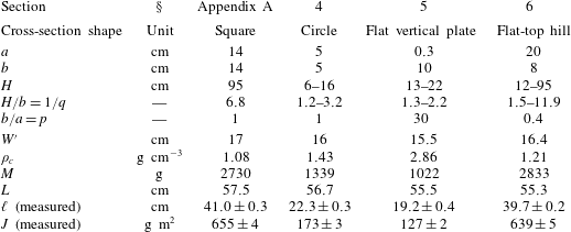
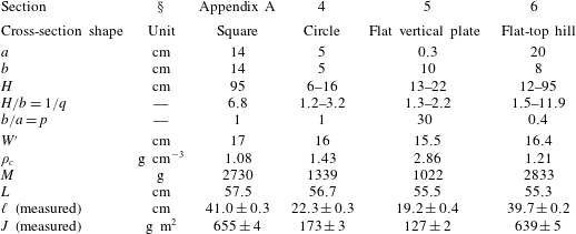
Parameters of the four cylinders used in the different sections of this paper. The shape indicates the cross-section of the cylinder in the $x{-}z$ plane. $a$ (respectively $b$ ) corresponds to the horizontal (respectively vertical) dimension of the cross-section. The fluid depth $H$ indicates the range of depths explored in this paper. $W^{\prime }$ is its width in the $y$ -direction and $\unicode[STIX]{x1D70C}_{c}$ its density. $M$ is the total mass of the pendulum and the cylinder, without the counter weight. $L$ and $\ell$ are defined in figure 2 while $J$ is the moment of inertia of the whole pendulum (without the counter weight). Note that $J$ and $\ell$ are carefully measured in air. The horizontal line in the middle of the table separates the parameters that determine the added mass (top) to the ones that are simple characteristics of the cylinders used (bottom).

The lower end of the pendulum with the cylinder is immersed at mid-depth of a stably density stratified fluid of depth $H$ , contained in a tank also sketched in figure 2. Two tanks were used to achieve different fluid depths. Experiments with $H=95$  cm were performed in a rectangular test tank of size $200\times 17\times 100~\text{cm}^{3}$ while the experiments with all the other fluid depths were conducted in a rectangular tank of size $160\times 17\times 42.5~\text{cm}^{3}$ . The tank is filled with uniformly stratified fluid using the conventional double-bucket technique and using salt as a stratifying agent. The density profile is measured prior to experiments by a conductivity probe attached to a vertical traverse mechanism. The value of the buoyancy frequency $N$ is evaluated from the measured density profile. Note that the volume of the immersed streamlined part of the pendulum is less than $1\,\%$ of the volume of the cylinder. Thus, one can neglect its influence on the fluid–body interactions. The cylinder has a width $W^{\prime }$ slightly smaller than $W$ , the width of the tank, to avoid friction on the lateral walls of the tank. For experiments performed with a small depth, the frequency of the surface seiche modes of the tank can be close to the characteristic frequency of the pendulum $\unicode[STIX]{x1D714}_{c}$ . Thus, it is possible to have an energy transfer from the pendulum to the surface seiche modes. A rigid lid placed on the free surface prevents the surface wave propagation and thus eliminates the energy transfers.

The pendulum is supported by an assembly which is fixed upon the tank. The rotation is made possible by two wedge-shaped supports made of very strong steel attached to the pendulum. Each wedge is in contact with a horizontal cylinder made of steel, oriented perpendicularly to the rib of the wedge and fixed on the assembly. With this arrangement, the friction at the contact points can be safely neglected. The rotation of the pendulum is limited to very small angles so we can consider the motion of the cylinder as horizontal. This is shown by the two thick arrows in the centre of the body in figure 2.

The horizontal displacement $x$ of the cylinder is measured as a function of time using a laser and a position sensor, assuming the pendulum oscillates within very small angles. Experimentally, we took care to limit the forcing in order to have a maximal horizontal displacement of $1$  cm. The laser spot is reflected on a small mirror, fixed on the pendulum and located on the axis of rotation. These small details are not shown in figure 2. As the pendulum oscillates, the mirror deflects the laser beam by an angle twice larger than the angular displacement. The deviation is measured via an elongated position sensor, giving a voltage proportional to the deviation of the laser spot. The deflection of the laser beam is recorded at a frequency of $50$  Hz during the experiment. Using the angular displacement and the distance $L$ between the rotation axis and the centre of mass of the cylinder, one can get the horizontal displacement  $x$ .

To prevent the internal wave reflection, wave absorbers are placed at each end of the tank (see figure 2). They are composed of a network of five layers of grids with two different mesh sizes, $3$ and $1$  cm. The space between the grids is approximately $5$  cm.

3.2 Data acquisition procedure and impulse response function analysis

Experiments have been performed with four different cylinders and for a set of different fluid depths. For each cylinder, the moment of inertia $J$ and the distance $\ell$ between the rotation axis and the centre of mass $G$ have been measured in air. Table 1 summarizes the different characteristics of the four cylinders used.

In a homogeneous or a stratified fluid, the equation of horizontal oscillations  $x$ of the centre of mass of the cylinder in the frequency domain can be written (Cummins Reference Cummins1962) as follows

with $C$ being the constant containing the effects of the pendulum torque and of the buoyancy force; $\unicode[STIX]{x1D707}(\unicode[STIX]{x1D714})$ is the inertial mass, $\unicode[STIX]{x1D706}(\unicode[STIX]{x1D714})$ the damping rate of the fluid and $F_{0}$ is the amplitude of forcing. For a homogeneous fluid, this rate is defined as $\unicode[STIX]{x1D706}_{h}$ and is only due to the viscosity of the fluid. For a stratified fluid, $\unicode[STIX]{x1D706}$ is the sum of the wave damping rate $\unicode[STIX]{x1D706}_{w}$ , due to emission of internal waves, and the viscous damping rate $\unicode[STIX]{x1D706}_{h}$ . The constant $C$ can be determined during a static calibration: the plate located on the right arm of the pendulum (see figure 2) is loaded with different masses $m$ . This causes a deviation of the equilibrium position of the pendulum. Thus, the two first terms of the left-hand side of (3.1) are null (static calibration) while the right-hand side is different from $0$ and depends on the masses $m$ and the geometry of the pendulum. Knowing everything except $C$ , we can measure this constant.

To determine $\unicode[STIX]{x1D707}$ and $\unicode[STIX]{x1D706}$ , we use the classical concept of impulse response function analysis (see e.g. Cummins Reference Cummins1962). The idea is to examine the response of the pendulum to a forcing proportional to $\exp (\text{i}\unicode[STIX]{x1D714}t)$ . The response function is defined by

Using (3.1) and (3.2), one has the complex quantity

Denoting $|R(\unicode[STIX]{x1D714})|$ its modulus and $\unicode[STIX]{x1D719}(\unicode[STIX]{x1D714})$ its phase, this leads to

where $|R(0)|$ stands for the modulus of the impulse response function for $\unicode[STIX]{x1D714}=0~\text{rad}~\text{s}^{-1}$ . As the system is linear, the normalization of $|R(\unicode[STIX]{x1D714})|$ by $|R(0)|$ allows us to use this Fourier transform approach at a small arbitrary impulse. For each position of the counter weights, experiments are repeated three times and three signals $x(t)$ are recorded. Each measurement appears to be very reproducible. Then, the Fourier transform of each of the three signals is calculated to obtain three impulse response functions, defined in (3.2). These three response functions are then averaged: the result is a complex function and its modulus and phase are computed. They are used to obtain the functions $\unicode[STIX]{x1D707}$ and $\unicode[STIX]{x1D706}$ as a function of the frequency $\unicode[STIX]{x1D714}$ . The impulse response function analysis allows us to measure $\unicode[STIX]{x1D707}$ and $\unicode[STIX]{x1D706}$ for a large range of frequencies but the measurements are accurate only around the characteristic frequency of the pendulum, $\unicode[STIX]{x1D714}_{c}$ . To increase the precision of the measurements of $\unicode[STIX]{x1D707}$ and $\unicode[STIX]{x1D706}$ as a function of the frequency, the different measurements performed at different positions of the counter weights are multiplied by a weight centred around the characteristic frequency $\unicode[STIX]{x1D714}_{c}$ . Thus, the different experiments are combined using the most reliable region of each measurement.

Always two series of experiments are performed, one in a homogeneous fluid first and then one in a stratified fluid. In the case of a homogeneous fluid, $\unicode[STIX]{x1D707}$ is supposed to be independent of the frequency and $\unicode[STIX]{x1D706}=\unicode[STIX]{x1D706}_{h}$ is expected to be proportional to $\sqrt{\unicode[STIX]{x1D714}}$ (Stokes Reference Stokes1851; Landau & Lifshitz Reference Landau and Lifshitz1959). The inertial coefficient $C^{\unicode[STIX]{x1D707}}$ is obtained by averaging $\unicode[STIX]{x1D707}$ in the sampled frequency range and using (2.8). The viscous damping is quantified by a linear fit of $\unicode[STIX]{x1D706}_{h}$ as a function of $\sqrt{\unicode[STIX]{x1D714}}$ . For the stratified case, the inertial coefficient $C^{\unicode[STIX]{x1D707}}$ as a function of frequency is obtained using (2.8). The wave damping rate $\unicode[STIX]{x1D706}_{w}$ is obtained by subtracting $\unicode[STIX]{x1D706}_{h}$ , previously measured in the homogeneous case, to $\unicode[STIX]{x1D706}$ . Then, the wave damping $C^{\unicode[STIX]{x1D706}}$ and radiated wave power $P_{w}$ coefficients are computed using (2.9) and (2.10). Finally, using the medfilt1.m Matlab function, we applied a median filter to $C^{\unicode[STIX]{x1D707}}$ and $C^{\unicode[STIX]{x1D706}}$ in order to slightly smooth the curves. The median filter has been performed on intervals of frequency $\unicode[STIX]{x1D714}$ of $0.05~\text{rad}~\text{s}^{-1}$ .

Note that the impulse response function analysis requires that the system is causal. Indeed, once the waves are emitted, they must not come back to the pendulum. Nevertheless, as the tank is limited in space, some waves are reflected at the ends of the tank and come back to the pendulum. Thus, they act as a source of oscillations and perturb the signal recorded. The wave absorbers, placed at each end of the tank to prevent the internal waves returning to the pendulum, are not fully efficient but limit the energy coming back to the pendulum. Note that wave reflections are more important when the frequency $\unicode[STIX]{x1D6FA}$ is low, i.e. when the waves propagate almost horizontally. In the following sections, to help the reader to identify quickly the range of frequencies where wave reflections are non-negligible in the experiments, the points showing the inertial, wave damping and radiated wave power coefficients are empty when reflections are important and filled when reflections are small or non-existent. The importance of the reflections is determined by using the different individual records $x(t)$ , not shown in this paper.

3.3 Set-up and data processing validation

A similar set-up and data processing method have been used in the previous works by Ermanyuk (Reference Ermanyuk2000, Reference Ermanyuk2002) and Ermanyuk & Gavrilov (Reference Ermanyuk and Gavrilov2002a ,Reference Ermanyuk and Gavrilov b , Reference Ermanyuk and Gavrilov2003). However, as the set-up and the method are similar but not strictly identical, we wanted to test them using previously published results. In order to do that, the first experiments have been performed using a cylinder with a square cross-section oscillating in a stratified fluid of large depth. Such experiments have already been reported by Ermanyuk & Gavrilov (Reference Ermanyuk and Gavrilov2002b ). In appendix A, we compare our results and the ones obtained in Ermanyuk & Gavrilov (Reference Ermanyuk and Gavrilov2002b ), showing a good agreement between the two sets of data. We also correct a small error in calculations present in Ermanyuk & Gavrilov (Reference Ermanyuk and Gavrilov2002b ). In the reminder of the manuscript, the set-up is used to address the effects of finite depth on tidal conversion.

4.1 Homogeneous fluid

The solution for the added mass coefficient of an elliptic cylinder submerged at mid-depth of a horizontal channel of homogeneous fluid has been obtained by Clarke (Reference Clarke2001)

where the parameter $\unicode[STIX]{x1D709}=\unicode[STIX]{x1D709}(p,q)$ is to be determined from the following equation

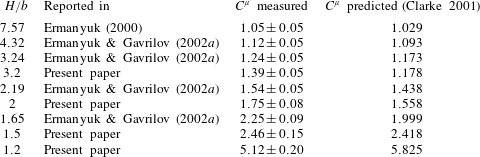
In our case, the cross-section of the cylinder is circular so that $p=1$ . Using (4.1) and (4.2), it is thus possible to compute the inertial coefficients in a homogeneous fluid as a function of $H/b$ . Table 3 gives the measured and predicted inertial coefficients $C^{\unicode[STIX]{x1D707}}$ for our four series of experiments and the five ones available in Ermanyuk (Reference Ermanyuk2000) and in Ermanyuk & Gavrilov (Reference Ermanyuk and Gavrilov2002a ). First, one can see that all the data sets are in a good agreement. Second, the prediction of Clarke (Reference Clarke2001) works well for high values of $H/b$ and remains reasonably accurate when $H/b$ decreases. Note that the numerical calculations of Sturova (Reference Sturova2001) lead to values close to the ones predicted by (4.1) and (4.2). Note also that the affine similitude theory cannot be used for predicting the added mass coefficients in the stratified case for $\unicode[STIX]{x1D6FA}<1$ because the prediction of Clarke (Reference Clarke2001) is not an analytical function. For $\unicode[STIX]{x1D6FA}>1$ , the prediction for the inertial coefficient are shown in figure 4 using dashed-dotted lines, with different colours corresponding to different fluid depths (see table 2).

Figure 3.

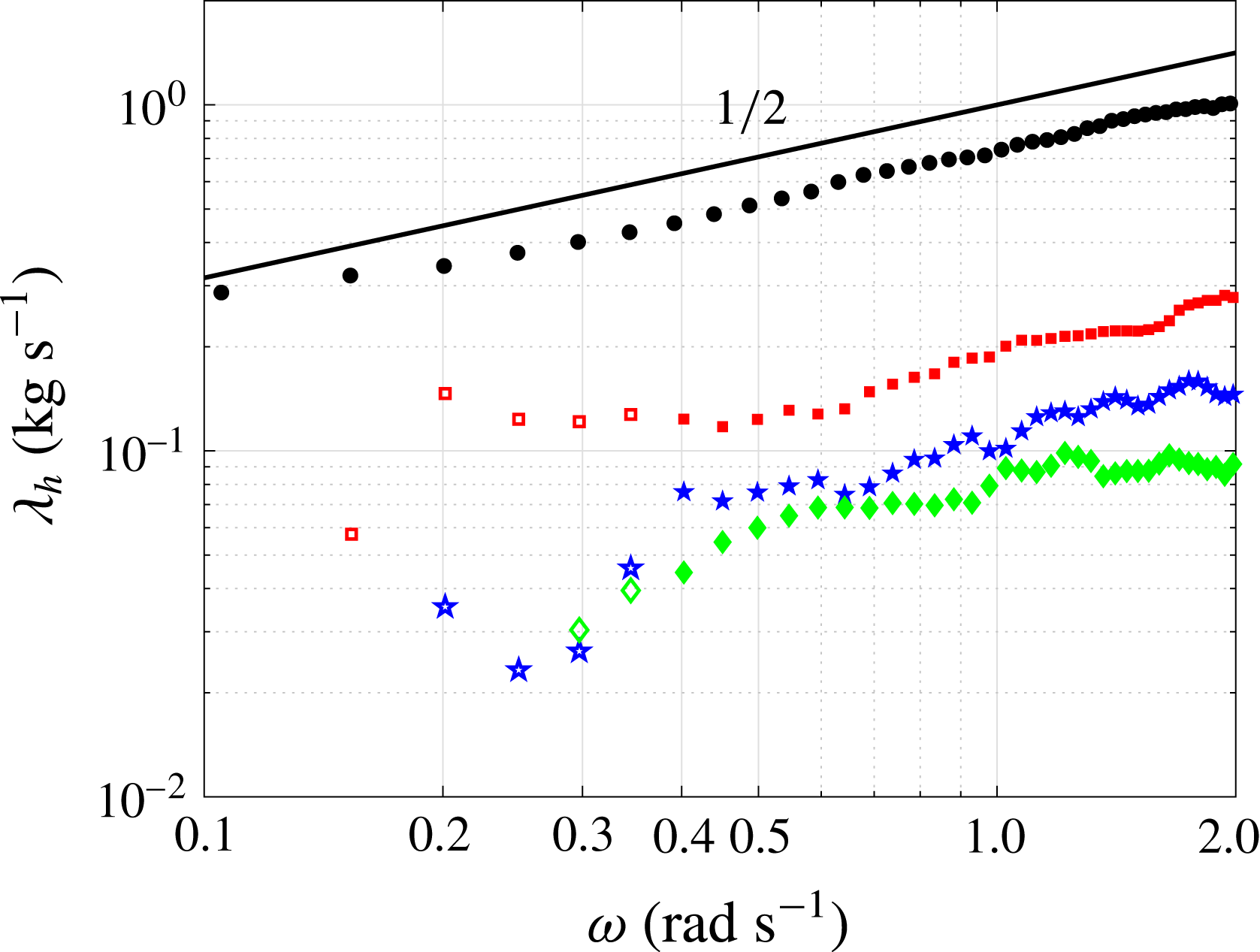
Homogeneous case: viscous damping rate $\unicode[STIX]{x1D706}_{h}$ as a function of frequency $\unicode[STIX]{x1D714}$ for the four series of experiments performed with our pendulum set-up in log–log scale. $H/b$ is equal to $1.2$ (black circles), $1.5$ (red squares), $2$ (blue pentagrams) and $3.2$ (green diamonds). The solid black line shows the power law $\unicode[STIX]{x1D706}_{h}\propto \sqrt{\unicode[STIX]{x1D714}}$ .

Table 3.

Measured (third column) and predicted (fourth column) inertial coefficients $C^{\unicode[STIX]{x1D707}}$ in a homogeneous fluid for the different $H/b$ ratios shown in the first column.

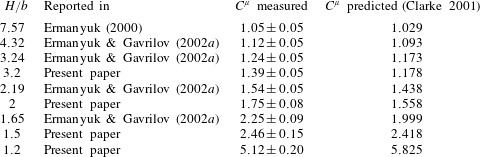
Figure 3 shows the viscous damping rates $\unicode[STIX]{x1D706}_{h}$ for the four series of experiments performed with the present pendulum set-up as a function of the frequency $\unicode[STIX]{x1D714}$ , in log–log scale. One can see that for frequencies higher than $\unicode[STIX]{x1D714}=0.5~\text{rad}~\text{s}^{-1}$ , the viscous damping rate $\unicode[STIX]{x1D706}_{h}$ agrees reasonably well with the square root of the frequency $\unicode[STIX]{x1D714}$ (Stokes Reference Stokes1851; Landau & Lifshitz Reference Landau and Lifshitz1959). Below $\unicode[STIX]{x1D714}=0.5~\text{rad}~\text{s}^{-1}$ , the signal is noisy except for the smallest value of $H/b$ (black filled circles). The different values of the coefficients $\unicode[STIX]{x1D706}_{h}/\sqrt{\unicode[STIX]{x1D714}}$ are reported in table 2.

4.2 Stratified fluid

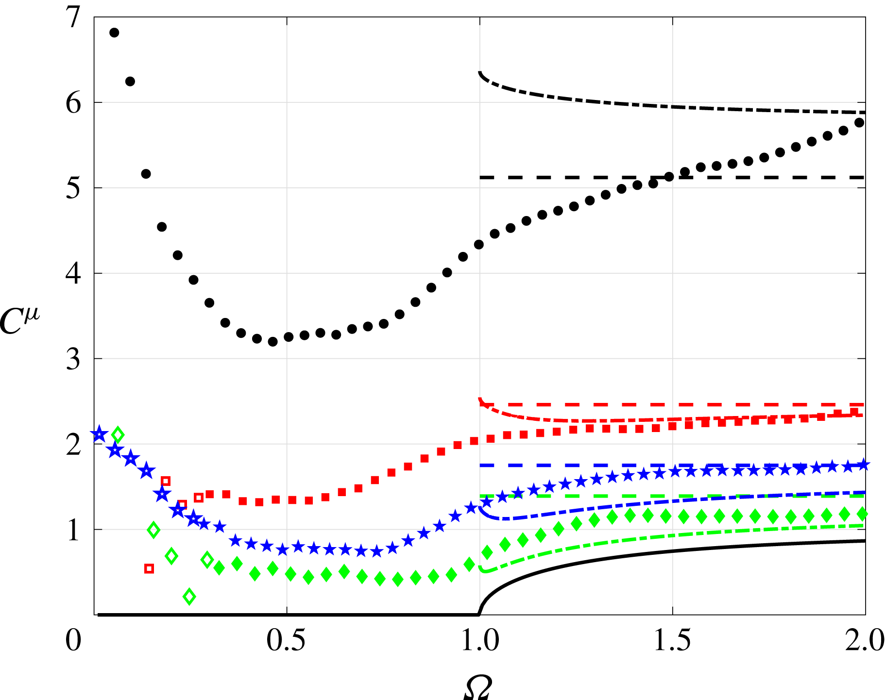
Figure 4 shows the inertial coefficients $C^{\unicode[STIX]{x1D707}}$ for the four series of experiments. The prediction made by Hurley (Reference Hurley1997) for a fluid of infinite depth is represented by the solid black line and the predictions from the affine similitude theory for finite depth are shown using the dashed-dotted lines. Note that for $\unicode[STIX]{x1D6FA}<1$ , the predicted inertial coefficient is identically zero for a fluid of infinite depth. In figure 4, one can see that the different inertial coefficients reach some asymptotic values for $\unicode[STIX]{x1D6FA}>1$ , except for the smallest $H/b$ ratio (black circles). These asymptotic values are close to the values measured in a homogeneous fluid, indicated by dashed lines. This is consistent with the prediction that, at high frequencies, the inertial coefficients are not different from the ones of the homogeneous case. The measurements are also in a relatively good agreement with the prediction of the affine similitude theory, except for $\unicode[STIX]{x1D6FA}$ close to $1$ where $\unicode[STIX]{x1D6FC}$ tends to $0$ . Even at $\unicode[STIX]{x1D6FA}>1$ the solution does not work well for vertically squeezed geometries, and therefore cannot be effectively used when $b/a=p$ is $O(1)$ and $H/b\rightarrow 1$ . One can note that as $H/b$ decreases, the inertial coefficient increases. Thus, the deeper, the smaller the inertial coefficient, at any frequency. This is consistent with the measurements performed by Ermanyuk & Gavrilov (Reference Ermanyuk and Gavrilov2002a ). At low frequency, the results are perturbed (see empty symbols) by wave reflections. Note that the range of frequency where the signal is noisy is reduced when one decreases the depth. Indeed, a small depth imposes to almost all waves to be reflected a given number of times at the top and bottom of the tank before reaching the ends of the tank. These multiple reflections induce a significant decay of waves.

Figure 4.

Stratified case: inertial coefficient $C^{\unicode[STIX]{x1D707}}$ as a function of the dimensionless frequency $\unicode[STIX]{x1D6FA}$ for the four different series of experiments at different depths. $H/b$ is equal to $1.2$ (black circles), $1.5$ (red squares), $2$ (blue pentagrams) and $3.2$ (green diamonds). The frequency range where wave reflections are important corresponds to the range where the symbols are empty. The horizontal dashed lines correspond to the inertial coefficient measured in a homogeneous fluid for the different depths. The solid black line corresponds to the theoretical prediction at infinite depth (Hurley Reference Hurley1997) and the dash-dotted lines represent the prediction made using the affine similitude theory, for $\unicode[STIX]{x1D6FA}>1$ . The colour code for lines is identical to the one for the symbols.

Figure 5.

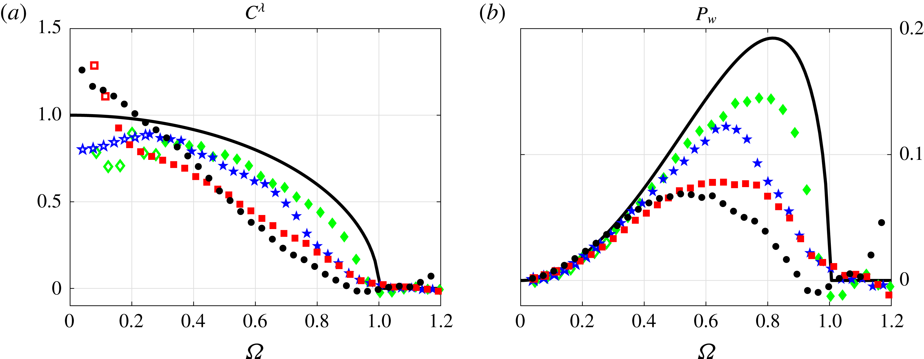
Stratified case: wave damping coefficient $C^{\unicode[STIX]{x1D706}}$ (a) and radiated wave power $P_{w}$ (b) as a function of the dimensionless frequency $\unicode[STIX]{x1D6FA}$ for the four different series of experiments at different depths. As in figure 4, $H/b$ is equal to $1.2$ (black circles), $1.5$ (red squares), $2$ (blue pentagrams) and $3.2$ (green diamonds). The frequency range where wave reflections are important corresponds to the range where the symbols are empty. The solid black line corresponds to the theoretical prediction at infinite depth (Hurley Reference Hurley1997).

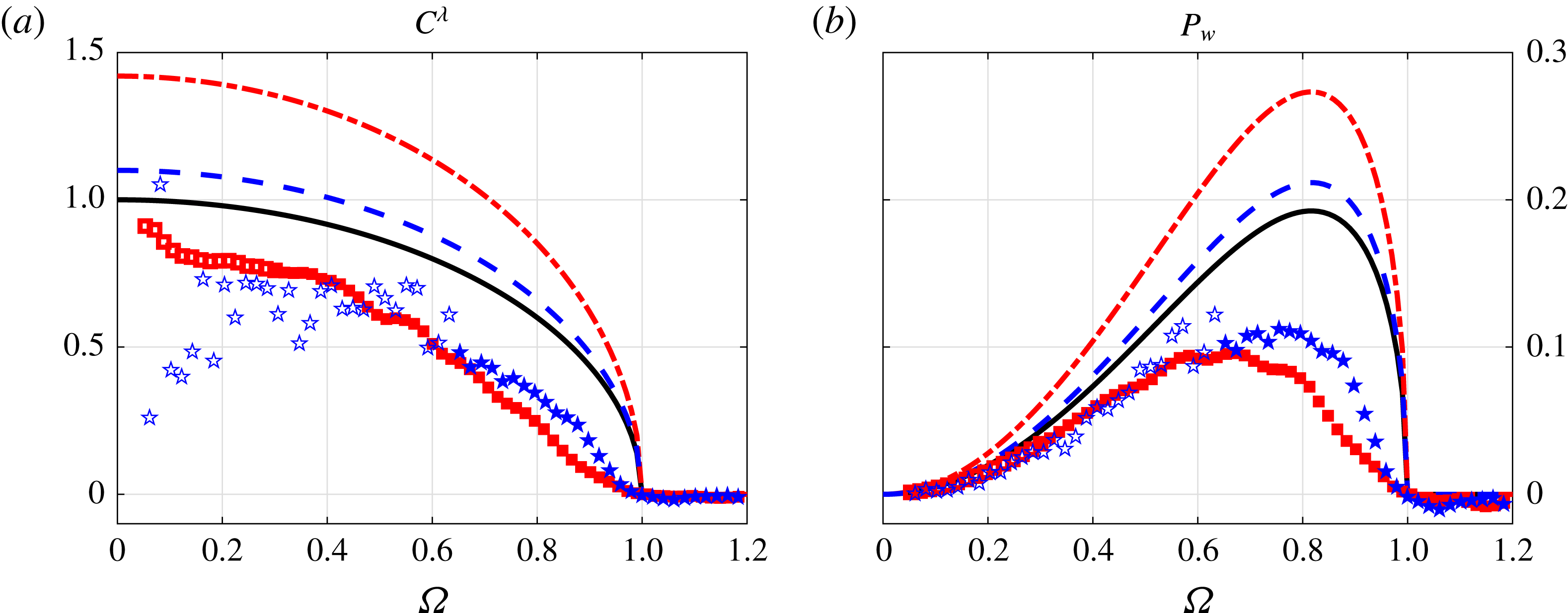
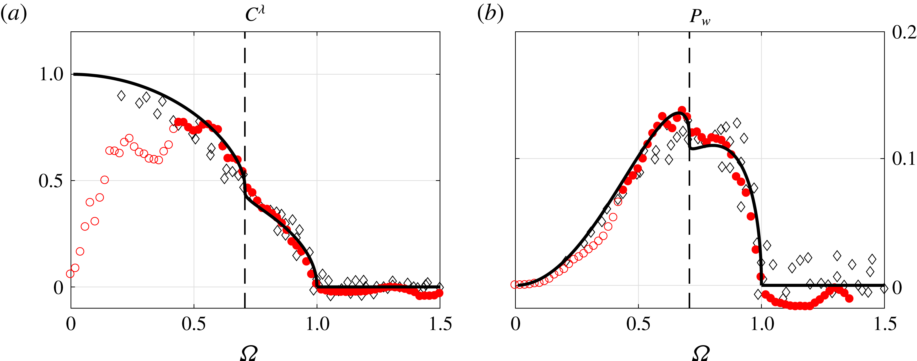
Figure 5 shows the wave damping $C^{\unicode[STIX]{x1D706}}$ and radiated wave power $P_{w}$ coefficients for the four series of experiments. The symbols used are the same as in figure 4 and are described in table 2. The prediction for a fluid of infinite depth (Hurley Reference Hurley1997) is plotted as a solid black line, on both panels. For $\unicode[STIX]{x1D6FA}>1$ , one can see that no wave is emitted and $C^{\unicode[STIX]{x1D706}}$ vanishes for all the four cases. In the studied range of $H/b$ , the efficiency of wave radiation in the frequency range $0.5<\unicode[STIX]{x1D6FA}<1$ drops systematically as the depth of fluid decreases. This behaviour is in qualitative agreement with Llewellyn Smith & Young (Reference Llewelyn Smith and Young2002) for a subcritical obstacle in a fluid of limited depth, and also with Gorodtsov & Teodorovich (Reference Gorodtsov and Teodorovich1986) and Ermanyuk & Gavrilov (Reference Ermanyuk and Gavrilov2002a ). However, at lower frequency, the opposite trend can be also observed (Llewellyn Smith & Young Reference Llewelyn Smith and Young2003): there is an enhancement of wave radiation at $H/b=1.2$ and $1.5$ at $\unicode[STIX]{x1D6FA}\rightarrow 0$ as expected for a supercritical obstacle, although it has a small magnitude in the case of a circular cylinder.

For a vertical plate, a fully supercritical case, one can expect that the force coefficients of a vertical plate are enhanced at $H/b\rightarrow 1$ for all frequencies $\unicode[STIX]{x1D6FA}$ . This issue is addressed in the next section.

5.1 Theoretical predictions

The added mass of a flat plate oscillating in a homogeneous fluid of infinite depth ( $H\rightarrow \infty$ and $q=b/H\rightarrow 0$ ) is $m_{A}=\unicode[STIX]{x1D70C}_{0}\unicode[STIX]{x03C0}b^{2}/4$ (see for example Brennen Reference Brennen1982). Therefore, the function given in (2.5) is $f_{\ast }(\infty ,0)\equiv 1$ . Thus, using the affine similitude theory, the inertial and wave damping coefficients in a linearly stratified fluid of infinite depth coincide with the solution found by Hurley (Reference Hurley1997), also valid for the cylinder having a circular cross-section (see § 4). Consequently, the non-dimensional wave power radiated by the flat plate in a uniformly stratified fluid of infinite extent amounts to

Note that the same result is true at finite $p=b/a$ since the added mass of an elliptic cylinder in the fluid of infinite extent depends only on its vertical size and does not depend on its elongation. This is in full qualitative agreement with Bell (Reference Bell1975).

Following Lockwood-Taylor (Reference Lockwood-Taylor1930), the added mass coefficient of a vertical flat plate of height $b$ oscillating in a homogeneous fluid of finite depth $H$ is

Thus, when $\unicode[STIX]{x1D6FA}<1$ , the wave power radiated by the flat plate in a uniformly stratified fluid of limited depth is

where we introduce the enhancement factor

Thus, the inertial and wave damping coefficients of a vertical plate oscillating horizontally in a fluid on finite depth are expected to be equal to the ones for a fluid of infinite depth multiplied by the enhancement factor  ${\mathcal{E}}$ . The above expression for the enhancement factor is equivalent to the result given by a more complicated formula in Llewellyn Smith & Young (Reference Llewelyn Smith and Young2003) (see equations (4.7) and (4.9) of this reference), with rotation neglected and taking into account a factor 2 since they consider only the upper half of the geometry. Explicitly, it means that

It is worth to note that the wave power given in Llewellyn Smith & Young (Reference Llewelyn Smith and Young2003) is in the low-frequency limit $\unicode[STIX]{x1D6FA}\rightarrow 0$ , where the dimensionless wave damping coefficient is given by

When $H\rightarrow \infty$ , we have $q\rightarrow 0$ and ${\mathcal{E}}\rightarrow 1$ . However, for smaller depths (or larger  $q$ ), ${\mathcal{E}}$ becomes greater than $1$ , which highlights a more important wave damping coefficient at finite depth than at infinite depth, in the low frequency limit relevant for the supercritical regime. Note also that the enhancement factor is the same both for the inertial coefficient $C^{\unicode[STIX]{x1D707}}$ at $\unicode[STIX]{x1D6FA}\rightarrow \infty$ and for the wave damping coefficient $C^{\unicode[STIX]{x1D706}}$ at $\unicode[STIX]{x1D6FA}\rightarrow 0$ . Following this theory, the inertial coefficient predictions are presented in figure 6, using solid lines while in figure 7(a), we show the theoretical prediction for the wave damping coefficient.

It is also possible to use the prediction of Clarke (Reference Clarke2001) by considering that the vertical plate has a shape close to a very elongated ellipse. As the thickness of the plate is very small, we have to take into account the viscous boundary layers, whose thickness $\unicode[STIX]{x1D6FF}$ can be of the same order of magnitude as that of the plate. It is given by

where $\unicode[STIX]{x1D714}$ is the frequency of the oscillations and $\unicode[STIX]{x1D708}$ the kinematic viscosity of the fluid. For frequencies of the order of $1~\text{rad}~\text{s}^{-1}$ , one gets $\unicode[STIX]{x1D6FF}\approx 0.2$  cm, which is close to the thickness of the plate. The theoretical curves for the inertial coefficient obtained using this method are represented in figure 6 for $\unicode[STIX]{x1D6FA}>1$ by dashed dotted lines. One can clearly see that the anticipated effect of the finite thickness of the vertical flat plate is low even if we add the ‘virtual’ boundary layer thickness on two sides of the plate $2\unicode[STIX]{x1D6FF}$ to the actual thickness of the plate $a$ . As in § 4, note that it does not seem possible to continue (4.1) and (4.2) to $\unicode[STIX]{x1D6FA}<1$ since the solution is not given by an explicit function.

Figure 6.

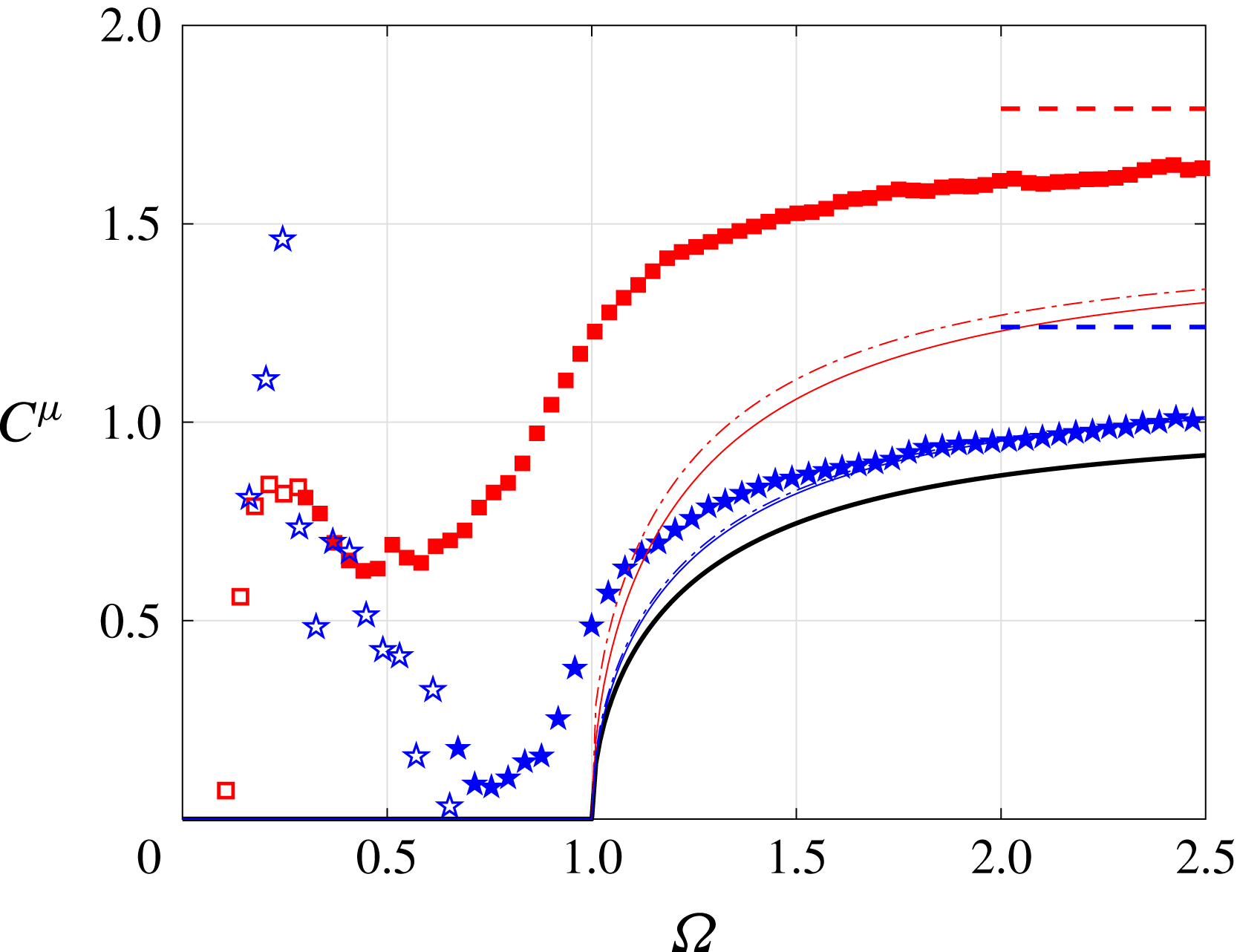
Stratified case: inertial coefficient $C^{\unicode[STIX]{x1D707}}$ as a function of the dimensionless frequency $\unicode[STIX]{x1D6FA}$ for the vertical flat plate at two different fluid depths. $H/b$ is equal to $2.2$ (blue stars) and $1.3$ (red squares). The frequency range where wave reflections are important corresponds to the range where the symbols are empty. The horizontal dashed lines correspond to the inertial coefficient measured in a homogeneous fluid for the two depths while the solid lines correspond to the theoretical prediction for a vertical plate and the dashed dotted lines to the theoretical prediction for a very thin ellipse. The colours are the same as the ones for the symbols. The black line represents the solution of Hurley (Reference Hurley1997) in a fluid of infinite depth.

Figure 7.

Stratified case: wave damping coefficient $C^{\unicode[STIX]{x1D706}}$ (a) and radiated power $P_{w}$ (b) as a function of the dimensionless frequency $\unicode[STIX]{x1D6FA}$ for the vertical flat plate at two different depths. As in figure 6, $H/b$ is equal to $2.2$ (blue stars) and $1.3$ (red squares). The frequency range where wave reflections are important corresponds to the range where the symbols are empty. The solid black line corresponds to the theoretical prediction at infinite depth made by Hurley (Reference Hurley1997) while the two coloured lines are obtained by multiplying this prediction by the enhancement factor corresponding to the two different series of experiments, according to (5.2).

5.2 Experimental results

Table 4 summarizes the results obtained in a homogeneous fluid for the vertical plate at two different depths. Similar to the case of a circular cylinder, the inertial coefficient $C^{\unicode[STIX]{x1D707}}$ and viscous damping rate $\unicode[STIX]{x1D706}_{h}$ increase as the depth decreases. The measured values of the inertial coefficient are typically $10\,\%$ – $20\,\%$ larger than the predicted ones.

Figure 6 shows the inertial coefficient $C^{\unicode[STIX]{x1D707}}$ as a function of $\unicode[STIX]{x1D6FA}$ for the vertical flat plate oscillating horizontally in a stratified fluid of limited depth. The symbols used here are described in table 4. For $H/b=2.2$ (blue pentagrams) and $\unicode[STIX]{x1D6FA}>1$ , the experimental and the two theoretical curves are close to each other, particularly for large frequencies. For $H/b=1.3$ , experimental points fall significantly above the theoretical curves. However, for both fluid depths, the inertial coefficient does not vanish for $\unicode[STIX]{x1D6FA}<1$ , contrary to the prediction. The inertial coefficient as a function of the frequency shows a very similar behaviour to the one for the circular cylinder (see figure 4). Note that, as in § 4, data are less reliable at small frequency due to the wave reflections. This is highlighted by empty symbols.

Figure 7 shows the wave damping $C^{\unicode[STIX]{x1D706}}$ and radiated wave power $P_{w}$ coefficients as a function of $\unicode[STIX]{x1D6FA}$ for the vertical flat plate. The symbols are the same as the ones used in figure 6 and are described in table 4. The enhancement factor given in (5.4) predicts that the wave damping coefficient and the radiated wave power at finite depth (coloured curves) are larger than the ones at infinite depth (solid black line), for all $\unicode[STIX]{x1D6FA}<1$ . This is obviously not the case here because both curves are below the prediction made by Hurley (Reference Hurley1997) for a fluid of infinite depth. Thus the cases of a flat plate and a circular cylinder show a similar behaviour (compare figures 5 and 7) even if the two bodies have different criticality. One can expect a wave damping coefficient larger than  $1$ at $H/b\rightarrow 1$ and $\unicode[STIX]{x1D6FA}\rightarrow 0$ , as predicted by Llewellyn Smith & Young (Reference Llewelyn Smith and Young2003) and seen in § 4. This is not the case here, despite a small ratio $H/b=1.3$ . It is difficult experimentally to go beyond and decrease this ratio. In the studied range of parameters we observed no enhancement for the wave damping coefficient of a flat plate at $\unicode[STIX]{x1D6FA}<1$ , despite the supercritical situation. The enhancement is however fully present for the inertial coefficient at $\unicode[STIX]{x1D6FA}>1$ .

As a plausible explanation, we may attribute the apparent absence of enhancement in wave damping coefficient in our experiments to the scale effect. Indeed the ideal-fluid theory (see figure 1 in Llewellyn Smith & Young Reference Llewelyn Smith and Young2003) considers the flow scheme with infinitely thin beams emanating from the tip of the vertical plate. The upward-emitted beams are reflected at the horizontal boundary and pass parallel and at small distance $2\unicode[STIX]{x1D6FF}\cos \unicode[STIX]{x1D703}$ from the downward-emitted beams, where $\unicode[STIX]{x1D6FF}$ is the height of the gap between the tip of the plate and the horizontal boundary. At laboratory scale the width of each beam in a viscous fluid is finite. This width can exceed the inter-beam distance $2\unicode[STIX]{x1D6FF}\cos \unicode[STIX]{x1D703}$ as $H/b\rightarrow 1$ . Therefore the beams can overlap, leaving a possibility of destructive interactions. A possible consequence for large-scale objects remains unclear since the width of beams at natural scale can be governed by turbulent viscosity (see for example Cole et al. Reference Cole, Rudnick, Hodges and Martin2009).

6.1 The shape of the object and theoretical prediction

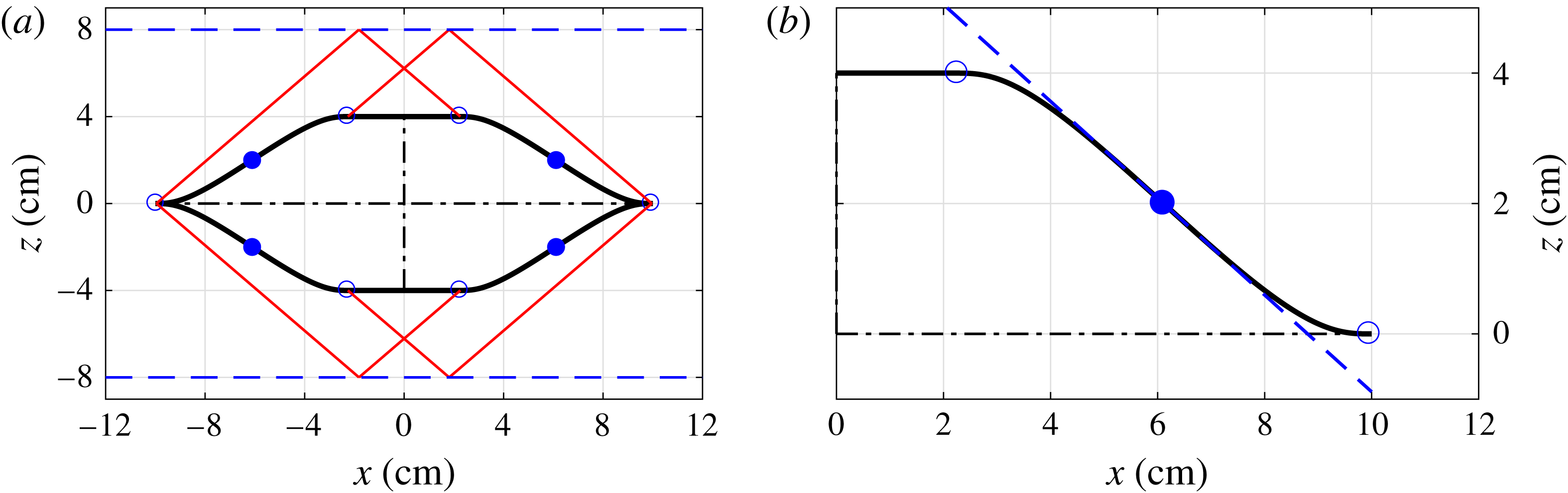
Figure 8(a) shows the shape of the object in the $x{-}z$ plane. Its height $b$ is equal to $8$  cm and it has a horizontal length $a$ of $20$  cm. The object is invariant in the $y$ -direction. As the shape is symmetric with respect to the $x$ and $z$ axes, it is composed of one specific curve shown in figure 8(b). The curve has a flat part for $x<2.26$  cm, with the limit marked by a blue circle. Then there is a decay with an inflection point, marked using a blue dot. At this inflection point, the slope has an angle of $36.6^{\circ }$ which corresponds to frequency of $\unicode[STIX]{x1D6FA}_{s}=0.596$ for internal waves. This slope is shown by a blue dashed line in figure 8(b). The inflection point has, by definition, the steepest slope of the curve. Another blue circle shows the end of the curve, close to $x=10$  cm. The two blue circles and the blue dot are shown on each side of the shape in figure 8(a).

Maas (Reference Maas2011) predicted that such a shape can exhibit a lack of tidal conversion for given frequency and depth. Indeed, if the depth is fixed, there can exist a specific frequency $\unicode[STIX]{x1D6FA}_{\ell }$ such that the two sides of the shape are connected by rays after a reflection at the surface or at the bottom. This is illustrated in figure 8(a) by the red lines showing internal wave rays and the dashed blue lines representing the surface and the bottom of the tank. With this geometry and at this specific frequency, the internal wave beams emitted by the pendulum are annihilated by pairs, after reflection on the surface or at the bottom of the tank, leading to a lack of tidal conversion. 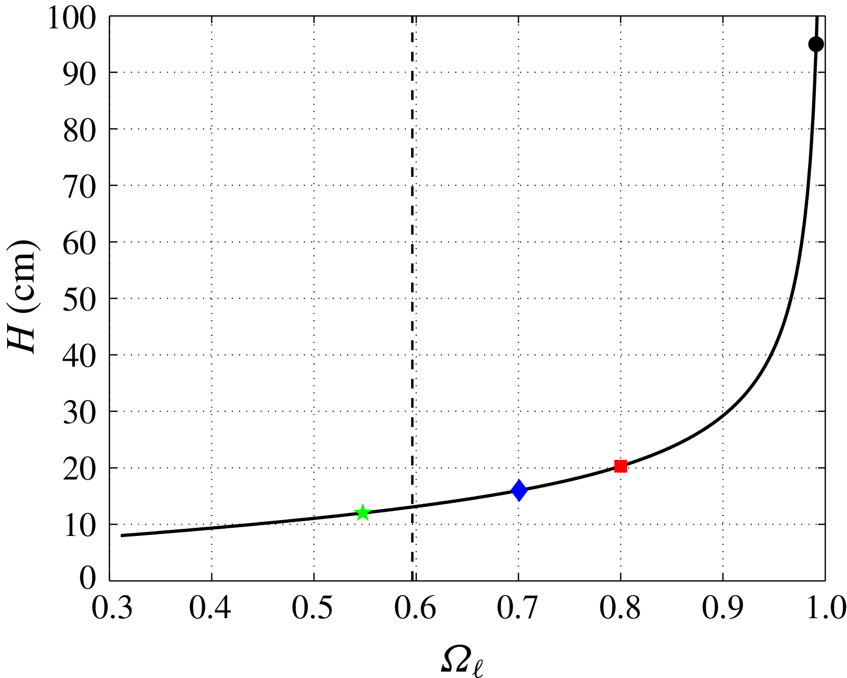When the fluid depth $H$ varies, the frequency corresponding to the lack of tidal conversion $\unicode[STIX]{x1D6FA}_{\ell }$ also changes. Figure 9 shows the height of the fluid $H$ as a function of the frequency $\unicode[STIX]{x1D6FA}_{\ell }$ . This frequency is much smaller than $1$ for small depth. When $H\rightarrow \infty$ , the dimensionless frequency $\unicode[STIX]{x1D6FA}_{\ell }$ shifts towards $1$ , i.e. the limit of the wave emission frequency range. Note that this is valid only for the frequency higher than $\unicode[STIX]{x1D6FA}_{s}$ , i.e. when the shape is subcritical. Indeed, one can easily understand that for $\unicode[STIX]{x1D6FA}<\unicode[STIX]{x1D6FA}_{s}$ , some internal wave rays should go through the object to connect the two sides of the shape. Thus, we should not observe a lack of wave emission for very small depths, for $H$ below $13$  cm.

Figure 8.

(a) Shape of the object in the $x{-}z$ plane (solid thick black line). The object is symmetric with respect to the $x$ and $z$ axes shown by the black dashed dotted lines inside. For this example, the cylinder is placed in the stratification of depth $H=16$  cm, limited by the two horizontal dashed blue lines. The red lines connect the two sides of the cylinder. (b) Zoom in on the upper right quarter of the object. The inflection point is marked by the blue point. The slope of the shape at this point is shown by the dashed blue line. The two blue circles show the portion of the shape which is not constant.

Figure 9.

Correspondence between the height of the fluid $H$ and the frequency where the topography lacks tidal conversion $\unicode[STIX]{x1D6FA}_{\ell }$ . The vertical dashed line shows the frequency $\unicode[STIX]{x1D6FA}_{s}=0.596$ . The four symbols represent the four different fluid depths reported in this paper.

In the next section, we discuss four series of experiments performed at $H=95$ , $20.3$ , $16$ and $12$  cm. These experiments are shown in figure 9 by the black circle, the red square, the blue diamond and the green pentagram, respectively. The prediction gives $\unicode[STIX]{x1D6FA}_{\ell }$ equal to $0.99$ , $0.8$ , $0.7$ and $0.55$ . Thus, we have explored the two different regions (subcritical and supercritical) in figure 9, separated by the dashed line at $\unicode[STIX]{x1D6FA}=\unicode[STIX]{x1D6FA}_{s}$ . Before performing these four series of experiments, the cylinder with this flat-top hill cross-section has been calibrated in the air. The main characteristics are presented in table 1. Note that due to the very specific shape of the body, there is no theoretical prediction for the inertial and wave damping coefficients.

Table 5.

Parameters for the four series of experiments with the flat-top hill cross-section. The inertial coefficient $C^{\unicode[STIX]{x1D707}}$ and the viscous damping rate $\unicode[STIX]{x1D706}_{h}$ are measured in the homogeneous case. The symbols in the last column are used in figures 10 and 11.

6.2 Experimental results

The inertial coefficient and viscous damping rate have been measured first in a homogeneous fluid using the impulse response function analysis. As expected, the inertial coefficient has been found constant for all frequencies and the viscous damping rate depends on the square root of the frequency. The results for the different fluid depths are shown in table 5.

Figure 10.

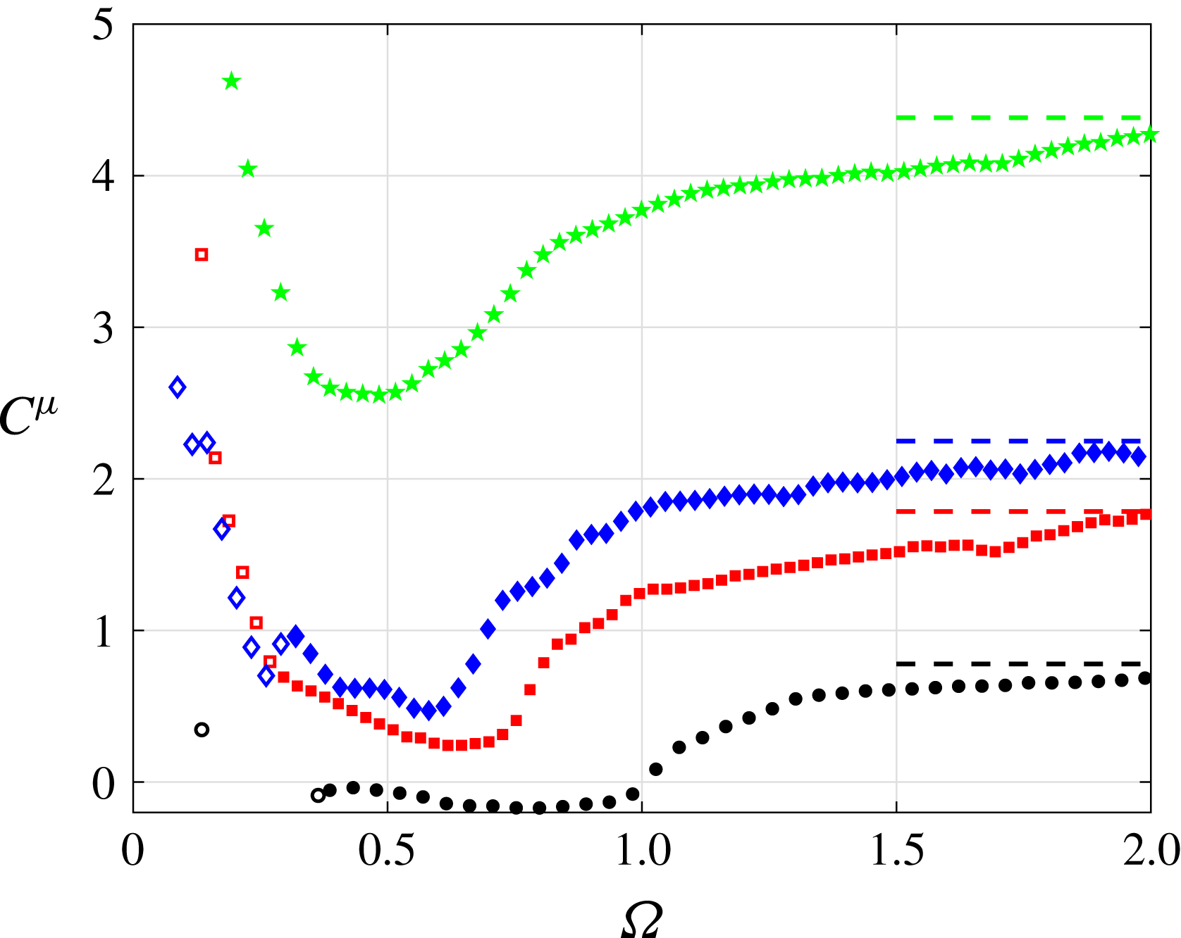
Stratified case: inertial coefficient $C^{\unicode[STIX]{x1D707}}$ as a function of the dimensionless frequency $\unicode[STIX]{x1D6FA}$ for the four different series of experiments at different depths. The symbols are indicated in table 5. The frequency range where wave reflections are important corresponds to the range where the symbols are empty. The horizontal dashed lines correspond to the inertial coefficient measured in a homogeneous fluid for the different depths. The colours are the same as the ones used for the symbols.

Figure 10 shows the inertial coefficients $C^{\unicode[STIX]{x1D707}}$ , for the four series of experiments. The different symbols are indicated in table 5. As for the cylinder with a circular cross-section and the vertical flat plate (see §§ 4 and 5), the inertial coefficient at smaller fluid depth is larger. Moreover, for large frequency, the inertial coefficients reach the asymptotic values found in the homogeneous fluid. These values are represented by horizontal dashed lines in figure 10.

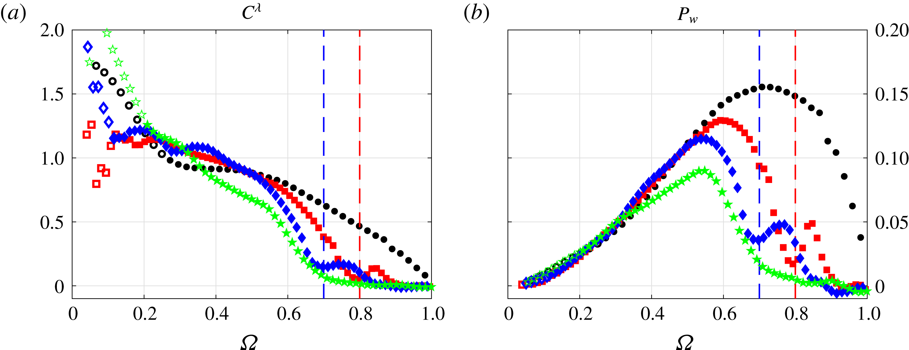
Figure 11 shows the wave damping and radiated wave power coefficients, for the four series of experiments. The different symbols are indicated in table 5. One can see a significant local minimum in these coefficients, at $\unicode[STIX]{x1D6FA}=0.8$ for $H=20.3$  cm (red squares) and at $\unicode[STIX]{x1D6FA}=0.7$ for $H=16$  cm (blue diamonds), while it is not the case for $H=95$  cm (black circles) and $H=12$  cm (green pentagrams). This is fully consistent with the theoretical prediction, given in figure 9. No minimum is seen for the infinite depth experiment, because the predicted frequency lacking of tidal conversion $\unicode[STIX]{x1D6FA}_{\ell }$ is too close to  $1$ . Moreover, for the supercritical topography ( $\unicode[STIX]{x1D6FA}<\unicode[STIX]{x1D6FA}_{s}$ ), there is no local minimum of tidal conversion. Note that the wave reflection at the end of the tank affects the signal only for $\unicode[STIX]{x1D6FA}$ smaller than $0.3$ so that the data in the frequency range of interest are fully reliable. Since the data corresponding $\unicode[STIX]{x1D6FA}<0.3$ are not reliable, we cannot make any conclusion concerning the enhancement of tidal conversion at $\unicode[STIX]{x1D6FA}\rightarrow 0$ for this type of topography.