

1. Introduction
Rayleigh–Taylor instability (RTI) (Rayleigh Reference Rayleigh1883; Taylor Reference Taylor1950) develops at the interface where a heavier fluid is accelerated by a lighter fluid, leading to the formation of bubbles (lighter fluid penetrating the heavier one) and spikes (heavier fluid penetrating the lighter one), often transitioning toward turbulence (Zhou et al. Reference Zhou, Clark, Clark, Glendinning, Skinner, Huntington, Hurricane, Dimits and Remington2019). The RTI poses a significant challenge in achieving net energy gain in inertial confinement fusion (Lindl et al. Reference Lindl, Landen, Edwards, Moses and team2014; Betti & Hurricane Reference Betti and Hurricane2016) and is crucial for understanding hydrodynamic mixing in astrophysical phenomena like a supernovae (Arnett Reference Arnett2000; Müller Reference Müller2020).
Significant focus has been placed on determining whether the late-time properties of RTI flows depend on the initial conditions (Zhou Reference Zhou2017a
,Reference Zhou
b
). When the interface is seeded with random small-scale perturbations dominated by high-order modes, the instability initially exhibits exponential growth, followed by saturation and a nonlinear self-similar regime governed by mode coupling (Haan Reference Haan1989; Dimonte Reference Dimonte2004). In an early work, Sharp (Reference Sharp1984) constructed a bubble amalgamation model for the RTI, predicting an average bubble rise velocity
 $\dot {a}^{{B}}$
 \begin{equation} \dot {a}^{{B}}\propto gt, \end{equation}
where
 $g$
is the acceleration. Youngs (Reference Youngs1984) exploited a self-similar modal growth of the RTI interface to arrive at the formula for bubble amplitudes
 $a^{{B}}$
and spike amplitudes
 $a^{{S}}$
 \begin{equation} a^{{B/S}}(t) = \alpha ^{{B/S}}Agt^2, \end{equation}
where
 $\alpha ^{{B}}$
and
 $\alpha ^{{S}}$
are the self-similar factors for bubbles and spikes, respectively, and
 $A$
is the Atwood number (
 $A=(\rho _{{h}}-\rho _{{l}})/(\rho _{{h}}+\rho _{{l}})$
, where
 $\rho _{{h}}$
and
 $\rho _{{l}}$
represent the densities of the heavier and lighter fluids, respectively). In these scenarios, the flow is generally believed to lose memory of its initial conditions and transition into self-similar mixing (Youngs Reference Youngs2013). However, the presence of long-wavelength perturbations in the initial spectrum can significantly influence late-time self-similar growth. Studies such as Ramaprabhu, Dimonte & Andrews (Reference Ramaprabhu, Dimonte and Andrews2005) and Youngs (Reference Youngs2013) demonstrate that long-wavelength perturbations result in larger
 $\alpha ^{{B}}$
compared with cases with short-wavelength perturbations. Despite these insights, experimental evidence remains limited due to the challenges in generating interfaces with precisely controlled initial conditions.
Alternatively, some initial conditions involve long-wavelength perturbations in the initial spectrum, with the amplitude of these perturbations influencing late-time self-similar growth (Youngs Reference Youngs2013). Ramaprabhu et al. (Reference Ramaprabhu, Dimonte and Andrews2005) observed that initial conditions with long-wavelength components lead to a logarithmic increase in
 $\alpha ^{{B}}$
as the initial amplitudes increase. In contrast, for cases with small random perturbations,
 $\alpha ^{{B}}$
shows no such dependence and stabilises at a universal lower bound of approximately
 $0.03\pm 0.003$
. This helps explain why most numerical simulations initialised with short-wavelength modes report lower
 $\alpha ^{{B}}$
values, as their evolution is governed solely by mode coupling. For instance, early experimental values of
 $\alpha ^{{B}}$
are relatively large, ranging from 0.05 to 0.08 (Read Reference Read1984; Youngs Reference Youngs1989; Dimonte & Schneider Reference Dimonte and Schneider1996, Reference Dimonte and Schneider2000), whereas numerical simulations typically yield values below 0.05. Olson & Jacobs (Reference Olson and Jacobs2009) studied RTI in miscible fluids with an Atwood number
 $A$
of 0.2. The initial conditions were classified as either ordered or disordered, and their results confirmed those of Ramaprabhu et al. (Reference Ramaprabhu, Dimonte and Andrews2005), showing that
 $\alpha ^{{B}}$
measurements in the mode-coupling regime are independent of initial amplitudes. Youngs (Reference Youngs2013) demonstrated that adding long-wavelength perturbations with a
 $k^{-3}$
(
 $k$
is the wavenumber) spectrum increases
 $\alpha ^{{B}}$
from approximately 0.025, typical in direct numerical simulations (DNS), to approximately 0.06, aligning with experimental results. Glimm et al. (Reference Glimm, Sharp, Kaman and Lim2013) conducted simulations consistent with experimental data, reconstructing initial conditions from Smeeton & Youngs’s (Reference Smeeton and Youngs1987) rocket experiments, which showed considerably weaker initial long-wavelength perturbations compared with the Texas
 $\mathrm{A}\&\mathrm{M}$
water channel experiments (Mueschke Reference Mueschke2008).
Dimonte (Reference Dimonte2004) explored the role of initial perturbations in linear electric motor (LEM) experiments (Dimonte & Schneider Reference Dimonte and Schneider2000), suggesting that these perturbations could enhance self-similar factors. He proposed that mode-coupling growth is a slow process, potentially accelerated by long-wavelength perturbations, and observed a weak logarithmic dependence of self-similar factors on the initial perturbation amplitudes. However, Glimm et al. (Reference Glimm, Cheng, Sharp and Kaman2020) disagreed, arguing that the effect of long-wavelength perturbations is too weak to significantly impact
 $\alpha ^{{B}}$
. They also criticised the analyses in Dimonte & Schneider (Reference Dimonte and Schneider1996) and Dimonte (Reference Dimonte2004), which highlighted the role of long-wavelength noise. More recently, Roberts & Jacobs (Reference Roberts and Jacobs2016) conducted experiments using both miscible and immiscible liquid combinations, where initial perturbations were generated by either background noise or parametrically forced Faraday waves at the interface. Their results showed that the specific form of the initial perturbations had no measurable effect on the self-similar factors. In contrast, miscibility was found to significantly influence self-similar factors, with much lower values observed in miscible experiments compared with immiscible ones. Overall, due to the challenges of generating interfaces with controllable initial conditions in experiments, the impact of initial perturbations on RTI remains uncertain, especially regarding the role of high-order modes in the growth of long-wavelength perturbations.
For incompressible Rayleigh–Taylor (RT) turbulence, the flow field becomes increasingly asymmetric as the Atwood number
 $A$
increases. Akula & Ranjan (Reference Akula and Ranjan2016) compared the self-similar factors from their gas channel experiments at
 $A \approx 0.73$
with those from Dimonte & Schneider’s (Reference Dimonte and Schneider1996) LEM experiments (
 $0.1 \lt A \lt 1.0$
) and Banerjee, Kraft & Andrews’s (Reference Banerjee, Kraft and Andrews2010) gas channel experiments (
 $0.03 \lt A \lt 0.6$
). The results showed that the self-similar factor for bubbles,
 $\alpha ^{{B}}$
, exhibits little variation with
 $A$
. In contrast, the self-similar factor for spikes,
 $\alpha ^{{S}}$
, shows a more complex dependency:
 $\alpha ^{{S}}$
is similar to
 $\alpha ^{{B}}$
for
 $A \leqslant 0.5$
, but as
 $A$
increases,
 $\alpha ^{{S}}$
rises sharply, becoming much larger than
 $\alpha ^{{B}}$
. Numerical studies using DNS have provided further insights into the behaviour of self-similar factors across different Atwood numbers. Livescu et al. (Reference Livescu, Ristorcelli, Petersen and Gore2010) found that
 $\alpha ^{{B}}$
values were nearly identical for
 $A = 0.04$
and
 $A = 0.5$
. Similarly, Cabot & Zhou (Reference Cabot and Zhou2013) observed that the self-similar factor for the total mixing width (
 $a^{{B}}+a^{{S}}$
), denoted as
 $\bar {\alpha }$
(defined by
 $a^{{B}}(t)+a^{{S}}(t)=\bar {\alpha }Agt^2$
), exhibited minimal dependence on
 $A$
across three DNS datasets with
 $A = 0.2$
, 0.5 and 0.8. Theoretically, Birkhoff (Reference Birkhoff1954) extended the single-mode theory (which characterises exponential growth to terminal velocity for bubbles) to multi-mode random perturbations with amplitudes comparable to their wavelengths, deriving
 $\alpha ^{{B}} = 0.06$
at
 $A = 1$
. While much of the previous research has focused on the dependence of
 $\alpha ^{{B}}$
on
 $A$
, the complex relationship between
 $\alpha ^{{S}}$
and
 $A$
remains an area requiring further investigation.
While two-dimensional (2-D) simulations of RTI are more computationally efficient than three-dimensional (3-D) simulations, it remains difficult to reliably translate insights from 2-D simulations to the 3-D context (Zhou Reference Zhou2017a
,Reference Zhoub). According to the Layzer-type model (Layzer Reference Layzer1955), 3-D RTI perturbations grow
 $\sqrt {3}$
times faster than their 2-D counterparts in the nonlinear regime (Mikaelian Reference Mikaelian1998; Goncharov Reference Goncharov2002). Youngs (Reference Youngs1991) conducted both 2-D and 3-D simulations of RTI-driven mixing of miscible fluids, observing that, in the early stages, the width of the mixing zone grows approximately 50 % faster in three than in two dimensions. However, in the later stages, as fully developed turbulence emerges, the 3-D growth rate slows and converges to an
 $\alpha ^{{B}}$
value similar to that of 2-D calculations. Oron et al. (Reference Oron, Arazi, Kartoon, Rikanati, Alon and Shvarts2001) demonstrated that the saturation time for growth rates in 3-D simulations is three times longer than in 2-D simulations, which aligns with experimental findings by Dimonte & Schneider (Reference Dimonte and Schneider2000). Cabot (Reference Cabot2006) observed notable differences in the flow characteristics between 2-D and 3-D RTI. In 2-D simulations, RTI flows display large chaotic columns and vortices predominantly composed of pure fluid, giving the impression of being more stirred than mixed. In contrast, 3-D simulations show a fully turbulent mixing region with fine-scale structures and extensive regions of mixed fluid. Additionally, Cabot (Reference Cabot2006) emphasised that, in the early stages, baroclinicity is the primary mechanism for generating enstrophy. However, at later times in 3-D flow, vortex stretching becomes the dominant mechanism. This term is absent in 2-D flow but plays a crucial role in 3-D turbulence by transferring energy and enstrophy from large to small scales. While much of the prior research on 2-D RTI has relied on simulations, experimental investigations remain limited. Comparative experiments on 2-D and 3-D RTI using consistent methodologies would be highly valuable.
Understanding the relationship between 2-D RTI flows and initial conditions remains a significant challenge, highlighting the need for innovative methods to create 2-D discontinuous gaseous interfaces with precisely controlled initial conditions. In this study, we used soap films to generate a 2-D RT-unstable interface featuring long-wavelength perturbations, superimposed by high-order modes, across various Atwood numbers. The evolution of RTI morphologies was captured through high-speed shadow photography. We performed experimental measurements of amplitude variations, Froude numbers and self-similar factors for bubbles and spikes, comparing our findings with results from other studies. A variation on the previously developed potential flow model was applied to quantify the influences of high-order modes and Atwood numbers on 2-D RTI.
Schematic illustrations of the top acrylic box with soap films (a), the experimental set-up (b) and high-speed shadow photography (c). fl in (c) is a short for focal length.

2. Experimental method
Soap films provide a distinctive and adaptable platform for investigating various fluid dynamics phenomena, owing to their ability to form thin, stable interfaces between different fluids or phases (Couder, Chomaz & Rabaud Reference Couder, Chomaz and Rabaud1989). The effectiveness of the soap film technique in generating a discontinuous interface between SF
 $_6$
and air for Richtmyer–Meshkov instability studies has been demonstrated by Liu et al. (Reference Liu, Liang, Ding, Liu and Luo2018) and Liang et al. (Reference Liang, Zhai, Ding and Luo2019b
, Reference Liang, Liu, Zhai, Ding, Si and Luo2021). This method significantly minimises the presence of short-wavelength disturbances and interface diffusion. Recently, Liang et al. (Reference Liang, Alkindi, Alzeyoudi, Liu, Ali and Masmoudi2024) utilised this technique to create a 3-D RT-unstable interface, adjusting the initial perturbation by varying the SF
 $_6$
concentration in the test gas. In this study, we apply the soap film technique for the first time to generate a 2-D RT-unstable interface with precisely controllable initial conditions.
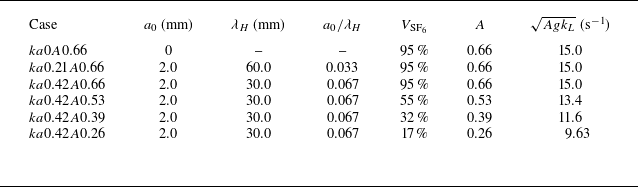
Physical parameters for 2-D RTI across various cases, where
 $a_0$
and
 $\lambda _{{H}}$
denote the initial amplitude and wavelength of the imposed high-order modes on the soap film interface,
 $V_{\mathrm{SF_6}}$
represents the volume fraction of SF
 $_6$
in the test gas within the top acrylic box,
 $A$
is the Atwood number and
 $\sqrt {Agk{L}}$
is the classical growth rate of RTI. Here,
 $g$
(
 $=9.79$
m s
 $^{-2}$
) is gravitational acceleration, and
 $k_{{L}}$
(
 $=34.9$
m
 $^{-1}$
) is the wavenumber associated with the long-wavelength perturbation.

To achieve this, we first constructed a transparent acrylic box with a sinusoidal open end, as shown in figure 1(a). The sinusoidal perturbation is mathematically described as
 \begin{equation} y=a_0\cos (k_{{H}}x), \end{equation}
where
 $a_0$
and
 $k_{{H}}$
represent the initial amplitude and wavenumber of the imposed high-order modes on the soap film interface. The ratio of the initial amplitude to the wavelength (
 $\lambda _{{H}}$
) of these high-order modes is kept below 0.1 in all cases, as detailed in table 1, ensuring the small perturbation assumption is met. The inner dimensions of the acrylic box are 6.0 mm in height and 180.0 mm in width, setting the wavelength of the long-wavelength perturbation on the soap film interface (
 $\lambda _{{L}}$
) to 180.0 mm. This high width-to-height ratio of the acrylic box helps suppress 3-D effects in the flow field. The wavelengths of high-order modes (60.0 and 30.0 mm) were selected as one third and one sixth of the long wavelength (180.0 mm), respectively, to ensure that the soap film interface remains perpendicular to the sidewalls, which act as symmetric boundaries. Sinusoidal filaments, matching the perturbation pattern of the acrylic box’s end and extending 0.1 mm into the flow, are attached to the box edges, as highlighted in red in figure 1(a). A rectangular frame, dipped in a soap mixture of 60 % distilled water, 20 % concentrated liquid soap and 20 % glycerine by volume, is then drawn along the sinusoidal filaments to form the soap film interface. Next, the top box, along with the aluminium frames, is aligned and connected with the bottom box, as depicted in figure 1(b). The top box is 220.0 mm tall, while the bottom box is 245.0 mm in height.
The SF
 $_6$
gas is introduced into the top box through a steel injection tube with an outer diameter of 1.0 mm, and displaced air exits through an oxygen (O
 $_2$
) detector. A gas regulator maintains a consistent SF
 $_6$
flow rate of
 $0.1\pm 0.02$
L min
 $^{-1}$
, resulting in a uniform SF
 $_6$
air mixture in the top box. The volume fraction of SF
 $_6$
(
 $V_{\mathrm{SF_6}}$
) in the mixture is determined by the equation
 $1-V_{\mathrm{O_2}}/0.22$
, where
 $V_{\mathrm{O_2}}$
is the volume fraction of O
 $_2$
measured by the detector, and 0.22 represents the O
 $_2$
concentration in air. Once the target
 $V_{\mathrm{SF_6}}$
level is reached, SF
 $_6$
injection is stopped, and the steel tube is gently lowered at a speed of approximately 0.01 m s
 $^{-1}$
, much slower than the growth rate of RTI. The sharp tip of the steel tube then punctures the soap film, triggering RTI driven by Earth’s gravity. The time between stopping SF
 $_6$
injection and puncturing the soap film is approximately 2 s, significantly shorter than the SF
 $_6$
injection duration. During this interval,
 $V_{\mathrm{O}2}$
readings from the O
 $_2$
monitor are continuously monitored. The observed
 $V_{\mathrm{O}2}$
value increases by no more than 0.01, matching the measurement error of the device. This study investigates 2-D RTI with
 $V_{\mathrm{SF_6}}$
ranging from 17 % to 95 %, corresponding to Atwood numbers
 $A$
between 0.26 and 0.66. The physical parameters of the initial 2-D unstable interface for various cases are detailed in table 1.
The flow field is recorded using high-speed shadow photography (as shown in figure 1
c), with illumination provided by a continuous light source. The high-speed camera (FASTCAM MINI WX) operates at a frame rate of 750 fps and a shutter time of 2.78
 $\unicode{x03BC}$
s. The resolution is
 $2048 \times 2048$
, giving a spatial resolution of 0.1 mm per pixel. The ambient pressure and temperature are 101.3 kPa and
 $293.5\pm 0.5$
K, respectively.
3. Results and discussion
3.1. Initial condition effects
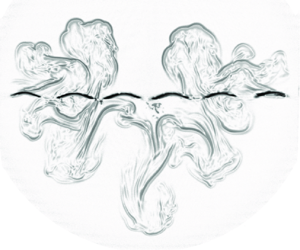
Figure 2 illustrates the evolution of 2-D RTI with
 $A=0.66$
under different initial conditions. The time zero (
 $t=0$
) marks the instant when the soap film ruptures at its centre. Using case
 $ka0A0.66\#1$
as an example, the deformation of an initially unperturbed SF
 $_6$
air interface is analysed in detail. To enhance the clarity of the interfacial morphology, background subtraction has been applied (see Appendix A). The thick black lines observed in the middle of the shadowgraphs are the sinusoidal filaments used to create the soap film interface. The rupture of the soap film triggers a broad perturbation in the surrounding gas as the rupture propagates outward from the puncture point (
 $t=67$
ms). The vortices are likely formed due to two main mechanisms: (i) during the rupture of the soap film, the thin film (
 $1\sim 10$
 $\unicode{x03BC}$
m thick) is replaced by the surrounding SF
 $_6$
and air, creating a dynamic flow pattern; and (ii) the ruptured soap film generates separate shear layers in the upper and lower gas regions, contributing to the observed vortical structures. This phenomenon is analogous to the sliding plate approach for RTI experiments described in previous studies (Duff, Harlow & Hirt Reference Duff, Harlow and Hirt1962; Linden, Redondo & Youngs Reference Linden, Redondo and Youngs1994).
Shadow images of the evolution of 2-D RTI in cases
 $ka0A0.66\#1$
,
 $ka0.21A0.66\#1$
and
 $ka0.42A0.66\#1$
.

In contrast to the symmetric evolution of bubbles and spikes characteristic of the linear regime in classical single-mode RTI, the early development in this study exhibits marked nonlinearity. After the film rupture, small vortices penetrate downward at the centre, while symmetric vortices rise on either side, maintaining reflective symmetry. These vortices play a critical role in the nonlinear evolution of the instability, as they enhance the mixing between the two fluids and contribute to the growth of bubbles and spikes. Over time, the small vortices in the top box merge into two large bubbles situated near the left and right edges of the visualisation window (
 $t=133$
ms). Simultaneously, vortices in the bottom box coalesce into a prominent central spike. As the system evolves, the bubbles rise further, while the spike’s head elongates into a finger-like structure (
 $t=200$
ms). Eventually, the spike’s head exits the visualisation window, and the bubbles expand horizontally along the
 $x$
-direction (
 $t=267$
ms).
A comparison of cases
 $ka0.21A0.66\#1$
and
 $ka0A0.66\#1$
reveals similar interface morphologies, with notable distinctions arising from the introduction of forced high-order modes in the former. In case
 $ka0.21A0.66\#1$
, the imposed modes with a wavelength of 60.0 mm result in a narrower primary spike accompanied by several smaller spikes. Additionally, the horizontal expansion of the two bubbles is less pronounced compared with case
 $ka0A0.66\#1$
. In contrast, case
 $ka0.42A0.66\#1$
exhibits a significantly different interfacial morphology. Following the soap film rupture, the forced high-order modes with a wavelength of 30.0 mm generate three downward-penetrating spikes and four upward-rising bubbles (
 $t=133$
ms). Over time, the central spike descends most rapidly, forming a mushroom-shaped head (
 $t=200$
ms), while the four bubbles merge into two larger bubbles near the edges of the visualisation window. These results highlight the substantial impact of forced high-order modes on the interfacial morphology in 2-D RTI, influencing the structure and dynamics of bubbles and spikes.
In comparison with Roberts & Jacobs (Reference Roberts and Jacobs2016), the flow in our study appears less mixed or turbulent. This distinction arises primarily from differences in the initial conditions and the dimensionality of the experiments. While Roberts & Jacobs (Reference Roberts and Jacobs2016) investigated 3-D RTI with multi-mode perturbations, leading to complex, turbulent mixing, our study focuses on 2-D RTI with controlled sinusoidal perturbations. This set-up results in fewer dominant modes and a more orderly flow evolution, significantly reducing the degree of chaos and promoting a more structured development of instability. Furthermore, the use of a soap film interface in our experiments suppresses diffusion and random short-wavelength disturbances, contributing to a more coherent and less mixed flow structure. These differences underscore the critical role of initial conditions and dimensionality in shaping the development and mixing characteristics of RTI.
Figure 3 presents the time-dependent bubble amplitudes
 $a^{{B}}$
and spike amplitudes
 $a^{{S}}$
measured across various experimental cases. The details of the measurement procedures can be found in Appendix A. Time is non-dimensionalised as
 $\tau = \sqrt {Agk_{{L}}}t$
, where
 $g = 9.79$
m s
 $^{-2}$
is the gravitational acceleration, and
 $k_{{L}} = 34.9$
m
 $^{-1}$
is the wavenumber associated with the long-wavelength perturbation of the soap film interface. The bubble and spike amplitudes are scaled as
 $\eta ^{{B/S}} = k_{{L}}(a^{{B/S}} - a_0)$
. Data from two independent experimental runs for each case (denoted
 $\#1$
and
 $\#2$
) are included. For clarity, error bars for the measured amplitudes, being smaller than the plot symbols, are omitted.
Time-varying dimensionless bubble amplitudes (a) and spike amplitudes (b) obtained from the experiments. The black lines represent predictions from the Zhang & Guo (ZG) model (3.2), while the red and blue lines correspond to predictions from the modified Zhang & Guo (mZG) model (3.4), and similarly hereinafter. The physical times for
 $\tau$
of 3.0 and 4.5 are 0.201 and 0.302 s, respectively.

Both
 $\eta ^{{B}}$
and
 $\eta ^{{S}}$
steadily increase across all cases due to the baroclinic mechanism. The convergence of
 $\eta ^{{B}}$
values across different cases suggests that RT bubble growth is independent of the high-order modes superimposed on the long-wavelength perturbation, consistent with previous findings (Roberts & Jacobs Reference Roberts and Jacobs2016). This is because the bubble growth is primarily driven by the buoyancy force, which dominates over the influence of small-scale perturbations. In contrast, the growth of
 $\eta ^{{S}}$
slows as the wavenumber of the imposed high-order modes increases, starting from an early stage (
 $\tau \gt 1.0$
), revealing a sensitivity of spikes to the initial conditions of the RT-unstable interface. This sensitivity has not been explicitly reported in previous studies, which often focused on initially random 3-D multi-mode perturbations or later stages of RTI evolution. By isolating and controlling the initial conditions in our 2-D set-up, we are able to uncover this previously overlooked dependency, providing new insights into the fundamental dynamics of RTI. Qualitatively, the spike head curvature decreases with increasing wavenumber of the imposed high-order modes, resulting in slower spike growth. Quantitatively, the growth of high-order modes saturates earlier than that of the long-wavelength perturbation (Haan Reference Haan1989, Reference Haan1991), advancing the onset of the RTI self-similar regime. Moreover, the saturated spike velocities associated with high-order modes are lower than the saturated velocity of the long-wavelength perturbation, thereby reducing the velocity of the prominent spike.
Layzer (Reference Layzer1955) introduced a potential flow model to describe late-time bubble velocities (
 $U^{{B}}$
) at
 $A=1$
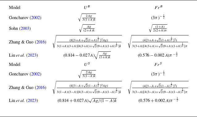
in the quasi-steady regime of RTI. This model was later generalised to arbitrary density ratios by Goncharov (Reference Goncharov2002) and Sohn (Reference Sohn2003). More recent extensions by Zhang & Guo (Reference Zhang and Guo2016) and Liu, Zhang & Xiao (Reference Liu, Zhang and Xiao2023) incorporated late-time spike velocities (
 $U^{{S}}$
) for arbitrary density ratios. Table 2 summarises the expressions for
 $U^{{B}}$
and
 $U^{{S}}$
from various studies on 2-D RTI. Previous numerical and experimental studies revealed that these models perform well in describing the evolution of bubbles, particularly in the nonlinear saturation stage. However, these models have limitations in describing the evolution of spikes, especially at high Atwood numbers, where the predicted curvature and growth rates deviate from experimental observations. These models assume potential flow, neglecting vorticity, which may not be valid for spike evolution, as spikes often develop complex vortex structures. In this study, we focus on analysing the discrepancies between the predictions of potential flow models and our experimental results, aiming to refine existing models by incorporating physical insights to better align with experimental data.
The expressions for the terminal bubble velocities (
 $U^{{B}}$
) and spike velocities (
 $U^{{S}}$
) in the quasi-steady regime, along with the corresponding Froude numbers for bubbles (
 ${Fr}^{{B}}$
) and spikes (
 ${Fr}^{{S}}$
). The theoretical model proposed by Zhang & Guo (Reference Zhang and Guo2016) is referred to as the ZG model.

Table 2 also includes the Froude number, a dimensionless parameter that quantifies the ratio of flow inertia to the external force field (gravity in this case). The table provides theoretical expressions for bubble Froude numbers (
 ${Fr}^{{B}}$
) and spike Froude numbers (
 ${Fr}^{{S}}$
). According to Ramaprabhu et al. (Reference Ramaprabhu, Dimonte, Young, Calder and Fryxell2006) and Wilkinson & Jacobs (Reference Wilkinson and Jacobs2007), these are defined as
 \begin{equation} {Fr}^{{B/S}}=\frac {\dot {a}^{{B/S}}}{\sqrt {Ag\lambda _{{L}}/(1\pm A)}}, \end{equation}
where
 $\dot {a}^{{B}}$
and
 $\dot {a}^{{S}}$
are the amplitude growth rates of bubbles and spikes, determined by differentiating
 $a^{{B}}$
and
 $a^{{S}}$
with respect to time. Figures 4(a) and 4(b) plot
 ${Fr}^{{B}}$
and
 ${Fr}^{{S}}$
against
 $\xi ^{{B}}$
(
 $=(a^{{B}} - a_0) / \lambda _{{L}}$
) and
 $\xi ^{{S}}$
(
 $=(a^{{S}} - a_0) / \lambda _{{L}}$
) for all experiments, with horizontal lines representing the theoretical predictions summarised in table 2.
The variations of the Froude numbers for bubbles,
 ${Fr}^{{B}}$
versus
 $\xi ^{{B}}$
(a), and for spikes,
 ${Fr}^{{S}}$
versus
 $\xi ^{{S}}$
(b). Symbols represent experimental results from various cases, while the lines show predictions from different models, and similarly hereinafter.

In figure 4(a), the experimental
 ${Fr}^{{B}}$
fluctuates around 0.30 from the beginning, indicating a rapid transition to a multi-mode structure following the soap film rupture, even for initially unperturbed or single-mode interfaces. This behaviour reflects the strong nonlinear dynamics in the early stages of RTI. The observed values are consistent with predictions from the potential flow model by Goncharov (Reference Goncharov2002) (
 ${Fr}^{{B}} \approx 0.33$
), as well as from Sohn (Reference Sohn2003), Zhang & Guo (Reference Zhang and Guo2016) and Liu et al. (Reference Liu, Zhang and Xiao2023) for
 $A=0.66$
. In contrast, figure 4(b) shows
 ${Fr}^{{S}}$
initially increasing from zero for
 $0 \lt \xi ^{{S}} \lt 0.4$
, then saturating at approximately 0.35 for
 $\xi ^{{S}} \gt 0.4$
. This behaviour highlights the asymmetry between bubbles and spikes. The experimental
 ${Fr}^{{S}}$
values match well with the predictions of Goncharov (Reference Goncharov2002), Zhang & Guo (Reference Zhang and Guo2016) and Liu et al. (Reference Liu, Zhang and Xiao2023) for
 $A=0.66$
when
 $\xi ^{{S}} \gt 0.4$
. Overall, while the late-time nonlinear behaviour observed in this study aligns with potential flow theory assuming inviscid and irrotational flows, the convergence of
 ${Fr}^{{S}}$
under varying initial conditions suggests that Froude numbers alone cannot fully capture the dependence of RTI on initial perturbations.
To describe the growth of long-wavelength perturbations for case
 $ka0A0.66$
, we utilise the potential flow model by Zhang & Guo (Reference Zhang and Guo2016) (ZG model). This model provides universal curves for both spikes and bubbles at any density ratio
 \begin{equation} \ddot {a}^{{B/S}}_{{L}}=-\epsilon ^{{B/S}}k_{{L}}\left[\left(\dot {a}^{{B/S}}_{{L}}\right)^2-\left(U^{{B/S}}_{{L}}\right)^2\right], \end{equation}
where
 $a^{{B/S}}_{{L}}$
represents the predicted amplitude of the long-wavelength perturbation for bubbles or spikes,
 $U^{{B/S}}_{{L}}$
is the late-time velocity of the bubble or spike for the long-wavelength perturbation (see table 2), calculated using the wavenumber
 $k_{{L}}$
, and
 $\epsilon ^{{B/S}}$
is dependent solely on
 $A$
, defined as
 \begin{equation} \epsilon ^{{B/S}}=\frac {3(1\pm A)(3\pm A)[4(3\pm A)+(9\pm A)\sqrt {2(1\pm A)}]}{4[3+A+\sqrt {2(1\pm A)}][4(3\pm A)+2\sqrt {2(1\pm A)}(4\mp 2A)]}. \end{equation}
The ZG model was initially developed to describe the 2-D RTI evolution, starting in the linear regime and progressing to a quasi-steady state. However, the RTI development becomes highly nonlinear after the rupture of the soap film interface. To address this, we reverse the timeline (applying the linear-regime model to negative time) as an equivalent infinitesimal perturbation and compute the ZG model’s predictions. These predictions, starting from a negative time of
 $-0.1$
ms with an infinitesimal perturbation at
 $A=0.66$
, are shown as black lines and align well with the experimental measurements of bubble and spike amplitudes.
The ZG model does not account for the influence of high-order modes, which play a significant role in the nonlinear evolution of RTI. To address this limitation, we introduce a modified version of the ZG model (mZG model) that decomposes the RTI growth into contributions from both high-order modes and long-wavelength perturbations. As demonstrated in Luo et al. (Reference Luo, Liu, Liang, Ding and Wen2020), significant mode coupling between long-wavelength and short-wavelength modes occurs when the long wavelength is twice the short wavelength. However, this coupling becomes negligible when the long wavelength exceeds three times or more the short wavelength. For cases
 $ka0.21A0.66$
and
 $ka0.42A0.66$
, the wavenumbers of the high-order modes are three times and six times those of the long-wavelength perturbation, respectively, leading to limited coupling between the short- and long-wavelength modes, which justifies the use of the linear sum approach. As a result, the mZG model is formulated as
 \begin{equation} a^{{B/S}}=a^{{B/S}}_{{L}}+a^{{B/S}}_{{H}}, \end{equation}
where
 $a^{{B/S}}_{{L}}$
and
 $a^{{B/S}}_{{H}}$
represent the predicted bubble/spike amplitudes for the long-wavelength perturbation and high-order modes, respectively. These amplitudes are given by
 \begin{align} \ddot {a}^{{B/S}}_{{L}} & =-\epsilon ^{{B/S}}k_{{L}}\left\{\left(\dot {a}^{{B/S}}_{{L}}\right)^2-\left[(1-\beta ) U^{{B/S}}_{{L}}\right]^2\right\},\nonumber\\[4pt] \ddot {a}^{{B/S}}_{{H}} & =-\epsilon ^{{B/S}}k_{{H}}\left[\left(\dot {a}^{{B/S}}_{{H}}\right)^2-\left(\beta U^{{B/S}}_{{H}}\right)^2\right].\\[-16pt] \nonumber \end{align}
Here,
 $\beta$
quantifies the contribution of high-order modes to the interfacial instability, with values ranging from 0 to 1. When
 $\beta = 0$
, the mZG model reduces to the original ZG model, describing the instability of an initially unperturbed interface. Conversely,
 $\beta = 1$
represents the scenario where long-wavelength perturbations are absent, which is unrealistic due to the inevitable presence of long-wavelength noise in experiments caused by spatial constraints (Dimonte & Schneider Reference Dimonte and Schneider1996; Dimonte Reference Dimonte2004). The late-time bubble/spike velocity of the high-order modes,
 $U^{{B/S}}_{{H}}$
, is calculated using the wavenumber
 $k_{{H}}$
. The values of
 $U^{{B/S}}_{{L}}$
and
 $U^{{B/S}}_{{H}}$
for cases
 $ka0.21A0.66$
and
 $ka0.42A0.66$
are provided in table 3. It is observed that the late-time velocities of both bubbles and spikes for high-order modes are smaller than those for long-wavelength perturbations. Moreover, as the wavenumber of the imposed high-order modes increases, the disparity between the late-time velocities of the high-order modes and the long-wavelength perturbations becomes more pronounced.
Theoretical late-time velocities for bubbles and spikes (
 $U^{{B/S}}_{{L}}$
) due to the long-wavelength perturbation, as well as late-time velocities for bubbles and spikes (
 $U^{{B/S}}_{{H}}$
) from high-order modes under various initial conditions. The expressions for late-time velocities can be found from ZG model in table 2. Here,
 $\beta$
represents the contribution of high-order modes to the interfacial instability, and in this study, it is set to 0.1. The dimensionless parameter
 $\delta$
is calculated using (3.6), with velocity expressed in units of m s
 $^{-1}$
.

The parameter
 $\beta$
is determined empirically based on the experimental data and reflects the relative importance of high-order modes in suppressing the growth of long-wavelength perturbations. For the cases studied here, we find that the mZG model predictions with
 $\beta =0.1$
provides the best agreement with the experimental results (see figure 3). This value indicates that high-order modes contribute approximately 10 % to the overall instability, while the remaining 90 % is driven by the long-wavelength perturbation. This decomposition allows us to capture the suppression of RTI growth due to high-order modes. Accounting for the contribution of high-order modes in the original ZG model results in a slight reduction in bubble amplitude growth and a more substantial decrease in spike amplitude growth. The suppressive effect of high-order modes is more pronounced in the case
 $ka0.42A0.66$
compared with
 $ka0.21A0.66$
. Overall, the mZG model demonstrates good agreement with experimental data for
 $\beta =0.1$
, confirming its validity for describing 2-D long-wavelength RTI with imposed high-order modes. The late-time velocities
 $(1-\beta ) U^{{B/S}}_{{L}}$
and
 $\beta U^{{B/S}}_{{H}}$
, as predicted by the mZG model for the cases
 $ka0.42A0.66$
and
 $ka0.21A0.66$
, are listed in table 3. The suppressive effect of high-order modes on 2-D long-wavelength spike growth can be estimated as
 \begin{equation} \delta =1-\frac {(1-\beta )U^{{S}}_{{L}}+\beta U^{{S}}_{{H}}}{U^{{S}}_{{L}}}. \end{equation}
As shown in table 3, the calculated
 $\delta$
values for cases
 $ka0.42A0.66$
and
 $ka0.21A0.66$
are 3.9 % and 5.6 %, respectively. These results indicate that the development of 2-D RTI is primarily dominated by the long-wavelength mode, while the suppressive effect of the imposed high-order modes remains secondary.
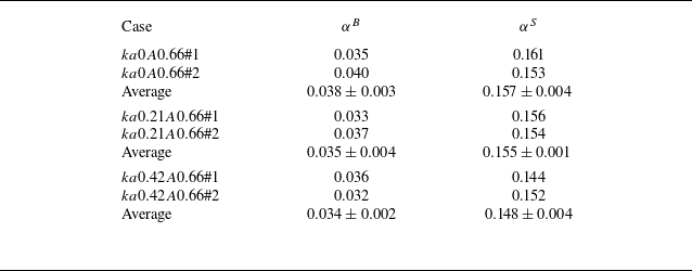
Measurements of self-similar factors for bubbles
 $\alpha ^{{B}}$
(a) and spikes
 $\alpha ^{{S}}$
(b) determined by a linear fitting to the
 $\sqrt {a^{{B}}}$
and
 $\sqrt {a^{{S}}}$
versus
 $t\sqrt {Ag}$
, and similarly hereinafter.

Turbulence is essential for self-similarity, so we calculated the maximum Reynolds number (Re) for the experiments: 20 000 for spikes and 7600 for bubbles, using the formula
 ${Re} = a^{{B/S}} \dot {a}^{{B/S}} / \nu$
, where
 $\nu$
is the weighted viscosity coefficient. The maximum Re values exceed the critical value of 3700 proposed by Dalziel, Linden & Youngs (Reference Dalziel, Linden and Youngs1999), justifying the discussion of self-similar factors for bubbles
 $\alpha ^{{B}}$
and spikes
 $\alpha ^{{S}}$
based on our experiments. The dependence of these self-similar factors on initial conditions is also explored. As noted by Banerjee et al. (Reference Banerjee, Kraft and Andrews2010), one method to determine
 $\alpha ^{{B}}$
and
 $\alpha ^{{S}}$
is to plot
 $\sqrt {a^{{B}}}$
and
 $\sqrt {a^{{S}}}$
against
 $t\sqrt {Ag}$
, as shown in figure 5. A straight line is then fitted (using the least squares method) to the linear portion of the curve at a later time (e.g. after a dimensionless time of 0.6 for bubbles in figure 5(a) and 0.4 for spikes in figure 5
b). Squaring the slope of this line provides an average value for
 $\alpha ^{{B}}$
and
 $\alpha ^{{S}}$
. The values of
 $\alpha ^{{B}}$
and
 $\alpha ^{{S}}$
under different initial conditions are listed in table 4. Our results show that both
 $\alpha ^{{B}}$
and
 $\alpha ^{{S}}$
values decrease slightly as the wavenumber of the imposed high-order modes increases, indicating that both bubble and spike evolution retains a weak memory of the initial conditions in the self-similar regime (Akula & Ranjan Reference Akula and Ranjan2016; Roberts & Jacobs Reference Roberts and Jacobs2016).
The values of the self-similar factors for bubbles (
 $\alpha ^{{B}}$
) and spikes (
 $\alpha ^{{S}}$
) under different initial conditions.

3.2. Atwood number effects
Figure 6 illustrates the evolution of 2-D long-wavelength RTI driven by high-order modes with a wavelength of 30.0 mm under different Atwood number conditions, ranging from 0.26 to 0.66. As the Atwood number decreases (indicating a smaller density difference between the two gases), the interface contours in the shadow images become lighter. For bubbles, a decrease in the Atwood number results in similar bubble heights, but with less horizontal expansion. For spikes, as the Atwood number decreases, the central spike’s height becomes more similar to that of the adjacent spikes, and it falls more slowly. For example, in case
 $ka0.42A0.66\#1$
, the head of the spike exits the visualisation window at
 $t = 267$
ms, while in case
 $ka0.42A0.26\#1$
, the spike head remains within the visualisation window. Overall, as the Atwood number decreases, the interfacial morphology becomes more symmetrical.
Shadow images of the evolution of RTI in cases
 $ka0.42A0.66\#1$
,
 $ka0.42A0.53\#1$
,
 $ka0.42A0.39\#1$
and
 $ka0.42A0.26\#1$
.

Time-varying bubble amplitudes
 $a^{{B}}$
and spike amplitudes
 $a^{{S}}$
are recorded from the experiments under various Atwood number conditions, as shown in figure 7. As the Atwood number decreases, the growth of both bubble and spike amplitudes slows down due to the smaller gravitational potential of the denser gas. Additionally, the difference between the bubble and spike amplitudes diminishes, indicating reduced nonlinearity in the 2-D RTI. For instance, in the case
 $ka0.42A0.66\#1$
at
 $t=0.2$
s, the spike amplitude is 0.089 m and the bubble amplitude is 0.049 m, resulting in a bubble-to-spike amplitude ratio of 1.84. In contrast, for the case
 $ka0.42A0.26\#1$
at
 $t=0.2$
s, the spike amplitude is 0.041 m and the bubble amplitude is 0.035 m, yielding a bubble-to-spike amplitude ratio of 1.19.
Time-varying bubble amplitudes (round symbols) and spike amplitudes (square symbols) measured from the experiments.

The time-dependent dimensionless bubble amplitudes
 $\eta ^{{B}}$
and spike amplitudes
 $\eta ^{{S}}$
are presented in figures 7(a) and 7(b), respectively. It is observed that, as the Atwood number decreases, the growth of
 $\eta ^{{B}}$
is slightly faster, while the growth of
 $\eta ^{{S}}$
slows down significantly. This indicates that the spike amplitude is more sensitive to the density ratio than the bubble amplitude. Additionally, the predictions from the mZG model (3.4) are shown as lines, matching the corresponding symbols in figures 7. The mZG model demonstrates agreement with the experimental data, confirming its applicability for quantifying the influence of high-order modes on the 2-D long-wavelength RTI across a wide range of Atwood numbers.
Time-varying dimensionless bubble amplitudes (a) and spike amplitudes (b) measured from the experiments. The physical times for
 $\tau$
of 3.0 and 4.5 for case
 $ka0.42A0.26$
are 0.311 and 0.467 s, for case
 $ka0.42A0.39$
are 0.258 and 0.387 s, for case
 $ka0.42A0.53$
are 0.224 and 0.335 s and for case
 $ka0.42A0.66$
are 0.201 and 0.302 s, respectively.

Figures 9(a) and 9(b) display
 ${Fr}^{{B}}$
versus
 $\xi ^{{B}}$
and
 ${Fr}^{{S}}$
versus
 $\xi ^{{S}}$
, respectively, with horizontal lines representing the theoretical predictions from the ZG model in table 2 for different Atwood numbers. The experimental values of
 ${Fr}^{{B}}$
under varying Atwood number conditions stabilise and oscillate around 0.30 from the start, while
 ${Fr}^{{S}}$
increases from zero and eventually saturates at approximately 0.35. It is observed that the Froude numbers for bubbles and spikes exhibit greater scattering as the Atwood number decreases. Additionally, the saturation of
 ${Fr}^{{S}}$
occurs earlier as the Atwood number decreases. The predictions from the ZG model for both
 ${Fr}^{{B}}$
and
 ${Fr}^{{S}}$
converge across different Atwood numbers.
The variations of the Froude numbers of bubbles
 ${Fr}^{{B}}$
versus
 $\xi ^{{B}}$
(a) and the Froude numbers of spikes
 ${Fr}^{{S}}$
versus
 $\xi ^{{S}}$
(b).

Measurements of self-similar factors for bubbles
 $\alpha ^{{B}}$
(a) and spikes
 $\alpha ^{{S}}$
(b).

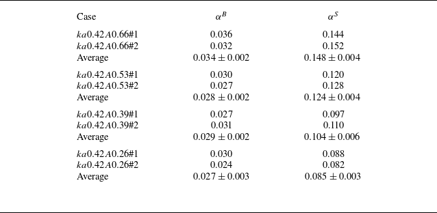
The dependence of the self-similar factors for bubbles
 $\alpha ^{{B}}$
, and spikes
 $\alpha ^{{S}}$
, on the Atwood number is examined through our experiments. Figures 10(a) and 10(b) show
 $\sqrt {a^{{B}}}$
and
 $\sqrt {a^{{S}}}$
plotted against
 $t\sqrt {Ag}$
, respectively. By squaring the slope of the linear fit, we obtain the averaged values for
 $\alpha ^{{B}}$
and
 $\alpha ^{{S}}$
. The values of
 $\alpha ^{{B}}$
and
 $\alpha ^{{S}}$
under different Atwood number conditions, along with their averages, are presented in table 5. The values of
 $\alpha ^{{B}}$
show weak dependence on the Atwood number, remaining around 0.03. In contrast,
 $\alpha ^{{S}}$
decreases significantly as the Atwood number decreases, indicating that spike evolution is strongly influenced by the density difference in the self-similar regime.
The values of the self-similar factors for bubbles (
 $\alpha ^{{B}}$
) and spikes (
 $\alpha ^{{S}}$
) in various cases and their averages.

Figure 11 compares the measurements of
 $\alpha ^{{B}}$
and
 $\alpha ^{{S}}$
versus Atwood numbers from previous 3-D experiments (Dimonte & Schneider Reference Dimonte and Schneider2000; Banerjee et al. Reference Banerjee, Kraft and Andrews2010; Akula & Ranjan Reference Akula and Ranjan2016; Roberts & Jacobs Reference Roberts and Jacobs2016), our 3-D experiments (Liang et al. Reference Liang, Alkindi, Alzeyoudi, Liu, Ali and Masmoudi2024), previous 2-D simulations (Youngs Reference Youngs1991; He, Chen & Zhang Reference He, Chen and Zhang1999; Liang et al. Reference Liang, Zhai, Ding and Luo2019a
) and the present 2-D experiments.
Self-similar factors of RT bubbles (
 $\alpha ^{{B}}$
) and spikes (
 $\alpha ^{{S}}$
) as a function of Atwood numbers. The markers represent results from various studies: Dimonte & Schneider (Reference Dimonte and Schneider2000) (square symbols), Banerjee et al. (Reference Banerjee, Kraft and Andrews2010) (delta-shaped symbols), Akula & Ranjan (Reference Akula and Ranjan2016) (gradient-shaped symbols), Roberts & Jacobs (Reference Roberts and Jacobs2016) (orange diamond-shaped symbols), Liang et al. (Reference Liang, Alkindi, Alzeyoudi, Liu, Ali and Masmoudi2024) (dark purple circle symbols), Youngs (Reference Youngs1991) (right-triangle-shaped symbols), He et al. (Reference He, Chen and Zhang1999) (left-triangle-shaped symbols), Liang et al. (Reference Liang, Hu, Huang and Xu2019a
) (cyan diamond-shaped symbols) and the present 2-D results (black circle symbols).

For bubbles, the
 $\alpha ^{{B}}$
values in the current 2-D results are smaller than most previous 3-D experimental studies, including the LEM experiments (Dimonte & Schneider Reference Dimonte and Schneider2000) and gas channel experiments (Banerjee et al. Reference Banerjee, Kraft and Andrews2010; Akula & Ranjan Reference Akula and Ranjan2016). However, they are close to recent miscible liquid experiments, both forced and unforced, with Faraday waves at the interface (Roberts & Jacobs Reference Roberts and Jacobs2016). Moreover, the current 2-D experimental values of
 $\alpha ^{{B}}$
are similar to three 2-D simulations at moderate Atwood numbers, including
 $\alpha ^{{B}}$
calculated by
 $a^{{B}}/Agt^2$
at the end of the fine mesh calculation (Youngs Reference Youngs1991) at
 $A=0.2$
, 0.5 and 0.9; 2-D RTI simulations using lattice Boltzmann scheme at
 $A$
of 0.5 (He et al. Reference He, Chen and Zhang1999); and high-resolution DNS of multi-mode immiscible RTI at
 $A$
of 0.1 (Liang et al. Reference Liang, Hu, Huang and Xu2019a
). This consistency demonstrates that 3-D effects are significantly suppressed in our experiments, with the interface morphology dominated by 2-D large-scale structures. Additionally, the
 $\alpha ^{{B}}$
values in the present 2-D experiments are smaller than those observed in our previous 3-D RTI experiments using a soap film interface. Since most of previous studies investigated RTI in 3-D flows, it is reasonable to conclude that the 2-D flows in this study lead to a smaller
 $\alpha ^{{B}}$
than prior work.
For spikes, we observe a similar trend, with the
 $\alpha ^{{S}}$
values in the present 2-D experiments being smaller than those in our previous 3-D RTI experiments, further confirming that 2-D flows result in smaller self-similar factors for spikes than 3-D flows. When the Atwood number is low (e.g.
 $A=0.26$
), the
 $\alpha ^{{S}}$
values in the current 2-D experiments are similar to those in the LEM (Dimonte & Schneider Reference Dimonte and Schneider2000) and gas channel experiments (Banerjee et al. Reference Banerjee, Kraft and Andrews2010; Akula & Ranjan Reference Akula and Ranjan2016). As the Atwood number increases, although the
 $\alpha ^{{S}}$
values rise in the results from Dimonte & Schneider (Reference Dimonte and Schneider2000) and Banerjee et al. (Reference Banerjee, Kraft and Andrews2010), the growth of
 $\alpha ^{{S}}$
in the present 2-D experiments is faster than in those previous studies. We were surprised to find that the values of
 $\alpha ^{{S}}$
in the work of Akula & Ranjan (Reference Akula and Ranjan2016) are weakly dependent of the Atwood number and even smaller than
 $\alpha ^{{B}}$
in the work of Roberts & Jacobs (Reference Roberts and Jacobs2016).
In our experiments, the use of the soap film technique results in an initially discontinuous interface. The initial thickness of the soap film is approximately
 $1{\sim}10$
 $\unicode{x03BC}$
m. Gas diffusion across the interface begins only after the soap film ruptures. By contrast, most prior RTI experiments employ an initial interface with a diffusive layer, where the density varies gradually between the two test fluids. For example, Roberts & Jacobs (Reference Roberts and Jacobs2016) estimated the thickness of this diffusion layer to be
 $0.5 \sim 1$
mm in their experiments. As discussed by Duff et al. (Reference Duff, Harlow and Hirt1962) and Mikaelian (Reference Mikaelian1982), the presence of a diffusion layer suppresses RTI growth. Additionally, since the surface energy is approximately one third of the potential energy difference between the gases (see Appendix B), the surface tension of the soap film may still influence RTI development. We hypothesise that the surface energy stored in the unruptured soap film enhances spike growth. These two factors lead to a larger
 $\alpha ^{{S}}$
in our study compared with previous work, particularly at higher Atwood numbers.
4. Conclusions
We conducted precise experiments on the 2-D RTI of an SF
 $_6$
air interface under Earth’s gravity. To effectively control the initial interface shape and eliminate diffusion layers, we employed a soap film technique to create a discontinuous gaseous interface. The impact of high-order modes on the growth of long-wavelength RTI perturbations was investigated by examining the RTI development under three initial conditions: one with an initially unperturbed interface and two with initially perturbed interfaces featuring different imposed high-order modes. Additionally, we explored the effect of the Atwood number on the asymmetry of bubbles and spikes.
The early development of RTI in this study exhibits significant nonlinearity. The growth of RT bubbles is unaffected by the high-order modes superimposed on the long-wavelength perturbation, consistent with previous findings (Roberts & Jacobs Reference Roberts and Jacobs2016). In contrast, the growth of RT spikes is sensitive to initial conditions and slows as the wavenumber of the imposed high-order modes increases. The analysis of the Froude numbers of bubbles and spikes reveals that various potential flow models (Goncharov Reference Goncharov2002; Sohn Reference Sohn2003; Zhang & Guo Reference Zhang and Guo2016; Liu et al. Reference Liu, Zhang and Xiao2023) predict identical results, which align well with our experimental observations. A modified nonlinear model (mZG model), based on the work of Zhang & Guo (Reference Zhang and Guo2016), was applied to quantify the suppression of RTI growth due to the imposed high-order modes. Beyond the critical Reynolds number for turbulence, the self-similar factors for bubbles (
 $\alpha ^{{B}}$
) and spikes (
 $\alpha ^{{S}}$
) exhibit weak dependence on initial conditions, indicating that bubble and spike evolution is memoryless on initial conditions in the turbulent flow.
The evolution of 2-D RTI was compared across four Atwood number conditions (0.26, 0.39, 0.53, 0.66). The dependence of the spike growth on the Atwood number is stronger than for bubbles. The Froude numbers for bubbles and spikes show more variation as the Atwood number decreases. In the self-similar regime,
 $\alpha ^{{B}}$
is weakly dependent on the Atwood number, while
 $\alpha ^{{S}}$
increases significantly as the Atwood number rises. Overall, the asymmetry of RTI becomes stronger as the density ratio between the two fluids increases. When comparing
 $\alpha ^{{B}}$
and
 $\alpha ^{{S}}$
values from this study with previous work, we conclude that the 2-D flows result in smaller values of
 $\alpha ^{{B}}$
and
 $\alpha ^{{S}}$
than 3-D flows. Due to the surface energy contained in the soap film and the eliminated gas diffusion and stratification, the
 $\alpha ^{{S}}$
growth is faster with increasing Atwood numbers in the present study compared with previous LEM and gas channel experiments (Dimonte & Schneider Reference Dimonte and Schneider2000; Banerjee et al. Reference Banerjee, Kraft and Andrews2010).
Funding
This work was supported by Natural Science Foundation of China (Nos.12388101 and 24FAA00998). Y.L. partially acknowledges the support from CAS Pioneer Hundred Talents Program.
Declaration of interests
The authors report no conflict of interest.
Appendix A. Background subtraction
Throughout the image sequence, we applied background subtraction to enhance the clarity of the interfacial morphology, excluding the image captured before the soap film rupture. As an example, figure 12 illustrates the background subtraction process for the image at
 $t=172$
ms in case
 $ka0.21A0.66\#1$
. We utilised the ‘Photron FASTCAM Viewer 4’ software to subtract the image at
 $t=0$
from the image at
 $t=172$
ms, applying a grey-scale threshold ranging from 0 to 10. This threshold was selected based on the noise level of the images to ensure that only significant interfacial features were retained. The background subtraction process involved pixel-wise subtraction, and the entire workflow was standardised to ensure reproducibility. To eliminate subjective bias, the grey-scale threshold was determined solely based on the noise characteristics of the images, and the same threshold was uniformly applied across all datasets.
The initial average position is indicated by a green dashed line in the post-processed image. In cases
 $ka0A0.66$
and
 $ka0.21A0.66$
, two primary bubble structures were identified. The distances between the initial average position and the highest points of these two bubbles were measured as bubble amplitudes
 $a_1^{{B}}$
and
 $a_2^{{B}}$
, as illustrated in figure 12. The bubble amplitude
 $a^{{B}}$
was then calculated as the average of these values:
 $a^{{B}}=(a_1^{{B}} +a_2^{{B}})/2$
.
Similarly, in cases
 $ka0.42A0.66$
,
 $ka0.42A0.53$
,
 $ka0.42A0.39$
and
 $ka0.42A0.26$
, four distinct bubble structures were observed. The distances between the initial average position and the highest points of these four bubbles were measured as
 $a_1^{{B}}$
,
 $a_2^{{B}}$
,
 $a_3^{{B}}$
and
 $a_4^{{B}}$
. The bubble amplitude
 $a^{{B}}$
was defined as the average of these four values:
 $a^{{B}}=(a_1^{{B}}+a_2^{{B}}+a_3^{{B}}+a_4^{{B}})/4$
.
In contrast, only one dominant spike structure was observed across all cases. The spike amplitude
 $a^{{S}}$
was defined as the distance between the initial average position and the lowest point of the spike.
Appendix B. Role of soap film shattering
High-speed movies of film rupture typically show a violent process involving droplet formation, ejection and rapid motion of the liquid sheet under the influence of surface tension. This process strongly resembles the popping of an inflated balloon. Ultimately, the bursting soap films adhere to the inner side of the observation window.
Sketch of the background subtraction process for experimental images.

Next, we compare the potential energy difference between low- and high-density gases with the surface energy contained in the soap film. For simplicity, we consider the high-density gas to be pure SF
 $_6$
and the low-density gas to be pure air. The potential energy of the gas can be calculated using the following equation:
 \begin{equation} E_{{p}}=\rho \Upsilon gh, \end{equation}
where
 $\rho$
is the density of the gas,
 $\Upsilon$
is the volume of the gas,
 $g$
is the gravitational acceleration and
 $h$
is the height of the gas’s mass centre. For SF
 $_6$
, the density is 6.413 kg m
 $^{-3}$
, the volume is
 $2.376\times 10^{-4}$
m
 $^3$
(
 $=0.220\times 0.180 \times 0.006$
m
 $^3$
), the mass centre height is 0.355 m and thus the potential energy is
 $5.18\times 10^{-4}$
J. Similarly, for air, the density is 1.204 kg
 $\cdot$
m
 $^{-3}$
, the volume is
 $2.646\times 10^{-4}$
m
 $^3$
(
 $=0.245\times 0.180\times$
 $0.006$
m
 $^3$
), the mass centre height is 0.1225 m and thus the potential energy is
 $3.90\times 10^{-5}$
J Consequently, the potential energy difference between the low- and high-density gases is
 $4.80\times 10^{-4}$
J. The surface energy contained in the soap film can be calculated using the following equation:
 \begin{equation} E_{{s}}=\sigma \Lambda , \end{equation}
where
 $\sigma$
is the surface tension coefficient, and
 $\Lambda$
is twice the surface area of the soap film. For simplicity, we assume the soap film is made of pure water and is flat. The surface tension coefficient of water is 0.0675 N m
 $^{-1}$
, and the surface area is
 $1.08\times 10^{-3}$
m
 $^{2}$
(
 $=0.18\times 0.006$
m
 $^{2}$
). Thus, the surface energy is
 $1.46\times 10^{-4}$
J. In summary, while the surface energy is approximately one third of the potential energy difference between the gases, the surface tension of the soap film may still influence RTI development. We hypothesise that the surface energy contained in the unburst soap film promotes spike growth.