




Non-technical Summary
Conodonts with conical elements that closely resemble Paleozoic species reappeared in the Early Triassic. The phylogeny, evolution, and paleoecology of these conodonts are poorly known. In this study, we describe a new species of Neostrachanognathus, N. koikei n. sp., one of the conical conodonts, and reconstruct the conodont apparatus of this species based on natural assemblages from the “Toishi-type” siliceous claystone of Japan. The apparatus of N. koikei consists of 15 elements, including two pairs of P, one pair of M, and four pairs of S elements, and a single S0 element. Notable features include conical P1 and P2 elements and nine S elements that are similar in morphology to each other. The S elements of N. koikei is identified as belonging to the form-species “Neohindeodella aequiramosa,” specifically to the morphology occurring from the Spathian to the Anisian. Furthermore, S elements of the type species of Neostrachanognathus, N. tahoensis, appear to correspond to “Neohindeodella benderi.” Therefore, judging from these S-element morphologies, we conclude that Neostrachanognathus belongs to the family Ellisoniidae. These conodonts with simplified elements flourished and were widely distributed throughout the world, from continental shelves to the open ocean, during the Early Triassic to the early Middle Triassic.
Introduction
Conodonts belonging to Neostrachanognathus Koike, Reference Koike1998 are uncommon in that they possess conical elements despite being Triassic taxa. When the type species, Neostrachanognathus tahoensis, was first described by Koike (Reference Koike1998), its apparatus was interpreted as consisting of four morphotypes of conical forms. Later, the discovery of natural assemblages of N. tahoensis revealed that the apparatus of the conodont contains 14 elements arranged in seven pairs. The elements in positions S1 to S4 are ramiform and have no element corresponding to S0, while the other three pairs of positions are occupied by coniform elements (Agematsu et al., Reference Agematsu, Orchard and Sashida2008). However, no other apparatus with such a composition is known, and its familial assignment and phylogenetic relationships remain unknown. Considering these problems, “N. tahoensis” has been used as a wastebasket taxon for Early Triassic coniform conodonts. Other than N. tahoensis, the forms Neostrachanognathus sp. A of Agematsu et al. (Reference Agematsu, Orchard and Sashida2008) from Oman and Neostrachanognathus sp. A of Leu et al. (Reference Leu, Bucher, Vennemann, Bagherpour, Ji, Brosse and Goudemand2022) from South China have been assigned to the genus. In addition, Muto et al. (Reference Muto, Takahashi, Yamakita and Onoue2020) revised the definition of Neostrachanognathus by redescribing Cornudina oezdemirae Gedik, Reference Gedik1975 as Neostrachanognathus oezdemirae and adding some records of “N. tahoensis” to its synonymy list. However, there are many morphological variations in these coniform elements, and their classification needs to be reconsidered.
Orchard (Reference Orchard2007), who summarized the classification and evolutionary history of Early Triassic conodonts, concluded that, except for surviving “Paleozoic lineages” that existed immediately after the Permian–Triassic boundary (PTB), after the Dienerian only the lineages of the superfamily Gondolelloidea and family Ellisoniidae persisted and dispersed, giving rise to Triassic conodonts. Although Neostrachanognathus is considered part of the superfamily Gondolelloidea, the 14-element composition mentioned above makes interpretation of the phylogenetic relationships of this group difficult (Orchard, Reference Orchard2007; Chen et al., Reference Chen, Krystyn, Orchard, Lai and Richoz2016). The Early Triassic was a period of environmental recovery after the PTB extinction, and it is important to clarify how conodonts experienced extinction and radiation during this period for studies of environmental change. In this study, we reconstruct the composition of the Neostrachanognathus apparatus and discuss the phylogenetic relationships of the genus based on new conodont natural assemblages from Itsuki Village, Kumamoto Prefecture, Japan. We also discuss the evolution and paleoecology of Neostrachanognathus during the Early Triassic.
Geological setting
In Itsuki Village, Kumamoto Prefecture, central Kyushu, rocks of the Kurosegawa, Southern Chichibu, and Shimanto belts (from north to south) strike generally northwest–southeast and dip to the northeast (Itsuki Village Comprehensive Academic Research Group, 1987; Ishida, Reference Ishida2009; Saito et al., Reference Saito, Takarada, Toshimitsu, Mizuno, Miyazaki, Hoshizumi, Hamasaki, Sakaguchi, Ohno and Murata2010). The Oritachi section of this study (32°23′58.54″N, 130°46′43.08″E; the “Oritate” section of Agematsu et al., Reference Agematsu, Orchard and Sashida2008) is in the Oritachi Valley, a tributary of the Itsuki-ogawa River, which flows through the southwestern part of the Itsuki area (Fig. 1). Chert and sandstone are exposed in the Oritachi Valley, along with small amounts of “Toishi-type” siliceous claystone (this term is explained in the Results section), siliceous mudstone, and mudstone (Fig. 1.2). Ishida (Reference Ishida2009) identified a chert–clastic rock sequence (Matsuoka, Reference Matsuoka1989) in the northeastern Itsuki area in which a stratigraphic sequence of chert, siliceous mudstone, and sandstone is structurally repeated three or four times because of thrusting. These cherts have been dated to the Middle Triassic to Middle Jurassic (Bajocian), and the clastic rocks to the Middle Jurassic to early Late Jurassic (Bajocian to Oxfordian) (Ishida, Reference Ishida2009). From these data, Ishida (Reference Ishida2009) correlated the rocks in the northeastern Itsuki area with the Momigi Unit (Saito et al., Reference Saito, Kimura, Naito and Sakai1996) of the Southern Chichibu Belt, which is part of a Jurassic accretionary complex. The Oritachi section is the southwestern extension of the study area of Ishida (Reference Ishida2009), so it is also considered to be comparable to the Momigi unit.
Geology of the Itsuki area. (1) Index map of Kyushu. (2) Geological map of the western part of the Itsuki area (modified after Saito et al., Reference Saito, Takarada, Toshimitsu, Mizuno, Miyazaki, Hoshizumi, Hamasaki, Sakaguchi, Ohno and Murata2010).
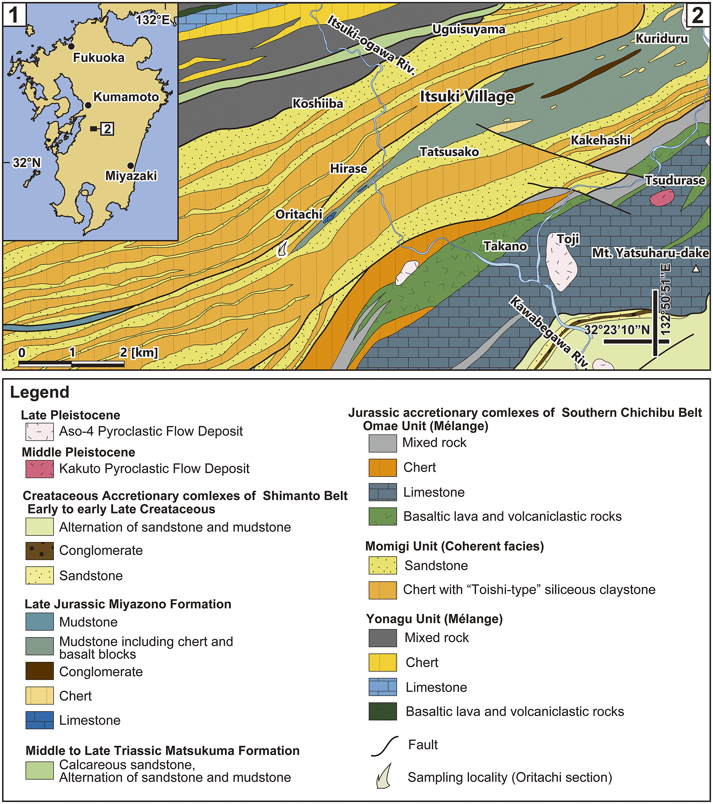
Figure 1. Long description
Panel 1, located in the top-left, is an index map of Kyushu island. It marks the cities of Fukuoka, Kumamoto, and Miyazaki. A small square labeled 2 indicates the study area location at approximately 32 degrees North and 132 degrees East.
Panel 2 is a detailed geological map of the Itsuki area. The Itsuki-ogawa River flows from the North toward the Southwest, and the Kawabegawa River flows from the Southeast toward the West. The map shows a series of Northeast to Southwest trending geological belts. The Northern and Central sections are dominated by the Momigi Unit, characterized by yellow-stippled sandstone and orange chert with Toishi-type siliceous claystone, featuring locations like Koshiiba, Itsuki Village, and Tatsusako. To the Northwest, the Omae Unit contains mixed rock, chert, and basaltic lava near Uguisuyama. The Southeast corner features the Yonagu Unit with dark grey limestone at Mt. Yatsuharu-dake and Toji, along with basaltic lava and volcaniclastic rocks near Takano. A sampling locality for the Oritachi section is marked with a white flame symbol in the Southwest. Black lines indicate faults cutting across the strata.
The Legend categorizes units by age. Late Pleistocene includes Aso-4 Pyroclastic Flow Deposit. Middle Pleistocene includes Kakuto Pyroclastic Flow Deposit. Cretaceous Accretionary complexes of Shimanto Belt include sandstone, conglomerate, and mudstone. Late Jurassic Miyazono Formation includes mudstone, chert, and limestone. Middle to Late Triassic Matsukuma Formation includes calcareous sandstone. Jurassic accretionary complexes of Southern Chichibu Belt are divided into the Omae Unit, Momigi Unit, and Yonagu Unit, each with distinct lithologies like chert, limestone, and mixed rock.
Microfossil analysis in the Itsuki area began with the report of Koike (Reference Koike1979), who examined cherts of the Sambosan Belt (equated with the Southern Chichibu Belt) in the Toji region and farther west, including the Oritachi section, and identified eight conodont assemblage zones covering the Spathian (lower Olenekian, Lower Triassic) to the Norian (Upper Triassic). In addition, Itsuki Village Comprehensive Academic Research Group (1987) obtained Spathian to Norian conodont fossils from limestone, chert, and “Toishi-type” siliceous claystone exposed at 36 sites in the Itsuki area. In that report, 10 species, including morphospecies, belonging to five genera from the “Toishi-type” siliceous claystone of the Oritachi section (Loc. CT-26 of Itsuki Village Comprehensive Academic Research Group, 1987) were illustrated. Agematsu et al. (Reference Agematsu, Orchard and Sashida2008) collected 33 samples of “Toishi-type” siliceous claystone and chert from the outcrop at this site and extracted conodonts from 17 samples. The claystones contain Cornudina igoi Koike, Reference Koike, Noda and Sashida1996, Triassospathodus symmetricus (Orchard, Reference Orchard1995), Neospathodus chionensis (Bender, 1967), and N. tahoensis and are assigned to the middle to upper Spathian. According to Agematsu et al. (Reference Agematsu, Orchard and Sashida2008), their floatstone sample A contains 15 natural assemblages of N. tahoensis and might have been derived from their 13s, 14, or 15s horizons.
Materials and methods
Lithostratigraphic analysis of the Oritachi section and microscopic observation of conodont fossils
In this study, a detailed lithostratigraphic analysis was conducted to estimate the stratigraphic level from which the natural assemblages of “Neostrachanognathus tahoensis” Koike, Reference Koike1998 of Agematsu et al. (Reference Agematsu, Orchard and Sashida2008) were obtained. In the field, we made a route map of the Oritachi Valley and drew columnar sections and outcrop sketches of the Oritachi section. In addition, rock samples were collected, mainly from the stratigraphic levels from which Agematsu et al. (Reference Agematsu, Orchard and Sashida2008) estimated the natural assemblage specimens were derived.
In the laboratory, we recovered conodont elements from rock samples and reexamined the rock samples collected by Agematsu et al. (Reference Agematsu, Orchard and Sashida2008). Conodont elements in siliceous claystone often have fine cracks and/or are compacted by consolidation, even when they appear to be well preserved, and may break if they are separated from the host rock by acid treatment methods. Therefore, following Sashida et al. (Reference Sashida, Kamata and Igo1992), rock samples were crushed into flakes or chips several millimeters to ~5 cm in size, and the elements on bedding planes were examined using a stereo microscope (Leica M165C, Leica Microsystems GmbH, Wetzlar, Germany) and a digital microscope (KEYENCE VHX-2000, KEYENCE Co., Ltd., Osaka, Japan) at magnifications of 30× to 120×.
Synchrotron radiation X-ray micro-tomography and three-dimensional modeling of a conodont natural assemblage
To reconstruct a conodont apparatus, it is necessary to observe the element arrangement of the conodont natural assemblage. However, it is not possible to extract elements while preserving this arrangement when the host rock is subjected to standard acid treatment; therefore, nondestructive element morphological analysis is required. We attempted to observe the morphology of the elements by synchrotron radiation micro-tomography (SR–μCT) of the natural assemblages and constructed three-dimensional (3D) models. Rock samples were observed under a stereomicroscope to preliminarily identify those samples containing natural assemblages or parts thereof. These samples were cut into small pieces of approximately 15 mm high, 5–10 mm wide, and 2–5 mm thick using a mini-router. The SR–μCT measurements were performed at experimental hutch 1 of BL20B2 in the synchrotron radiation facility, SPring-8, Hyogo, Japan (Goto et al., Reference Goto, Takeshita, Suzuki, Ohashi and Asano2001). The measurement conditions of the micro-tomography were based on Agematsu et al. (Reference Agematsu, Uesugi, Sano and Sashida2017, Reference Agematsu, Utagawa and Fukushima2023) and were as follows: X-ray energy of 35 keV; number of projections, 1,800 for 180°; exposure time for one projection, 200 msec; total scan time for one CT measurement, ~8 min; effective pixel size, 1.23–2.76 μm; and distance from sample to detector, 70 mm. The CT reconstruction was performed with the convolution back-projection method (Uesugi et al., Reference Uesugi, Hoshino, Takeuchi, Suzuki, Yagi and Nakano2010) after phase retrieval (Paganin et al., Reference Paganin, Mayo, Gureyev, Miller and Wilkins2002). Three-dimensional images were built from the stacked 2D images with volume rendering using the open-source visualization software ImageJ (https://imagej.nih.gov/ij/docs/faqs.html#cite), Drishti (Limaye, Reference Limaye and Stock2012; https://github.com/nci/drishti), and Avizo (https://cases.amira-avizo.com). Conodont elements are made of bioapatite, which is a biomineral that is compositionally similar to non-stoichiometric hydroxyfluorapatite (McMillan and Golding, Reference McMillan and Golding2019) and is generally considered to be denser than sedimentary rock. For example, the “Toishi-type” siliceous claystone in Itsuki has a density of ~2.6 g/cm3 (Agematsu et al., Reference Agematsu, Fukushima, Fujisaki and Ozeki2024). However, conodonts in “Toishi-type” claystones are often altered by diagenesis to a density similar to that of the host rock matrix, which may result in the conodont morphology being unrecognizable in 3D model constructions (Agematsu et al., Reference Agematsu, Fukushima, Fujisaki and Ozeki2024). In such cases, the tomographic image was viewed in ImageJ, and element outlines were carefully traced by hand. As a result of the above SR–μCT analyses, several natural assemblages were found, one of which was identified as Neostrachanognathus Koike, Reference Koike1998.
Repository and institutional abbreviation
The specimens studied in this paper are stored in the University of Tsukuba (IGUT-yf0001 to yf0017), Japan.
Results
Lithostratigraphy
The Oritachi section comprises, from bottom to top, black claystone (55 cm thick), “Toishi-type” siliceous claystone (135 cm thick) with a few thin chert layers, cherty siliceous claystone (30 cm thick) with a few chert layers, and bedded chert (980 cm thick), with a total thickness of ~12 m (Fig. 2). The general strike is N60–80°W, dipping 40–50°N. The lowermost black claystone has a very fine-grained matrix with a high content of organic matter and a well-developed bedding-parallel cleavage and is intensely sheared. Pyrite crystals are scattered or concentrated in lenticularly shaped clusters. Microfossils such as conodont elements are not present in this rock. The black claystone gradually changes to the “Toishi-type” siliceous claystone facies. The “Toishi-type” siliceous claystone has been used as a whetstone in Japan since around the Kamakura period (~800 years ago): “Toishi” means whetstone in Japanese (e.g., Muramatsu, Reference Muramatsu1973; Imoto, Reference Imoto1984). The claystone is dark gray, gray, pale gray, or weathered greenish gray in the Oritachi section. The matrix is composed mainly of microcrystalline quartz and clay minerals, and the texture is homogeneous. Moreover, the matrix contains conodont elements, often fragmented, and bead-like spherical radiolarian tests. The fossils can be observed on bedding-parallel cleavage planes.
Lithological column showing the stratigraphic distributions of conodonts in the Oritachi section. “Conodont natural assemblage” from the sampling horizon ORTC-007 includes IGUT-yf0002 and IGUT-yf0003.
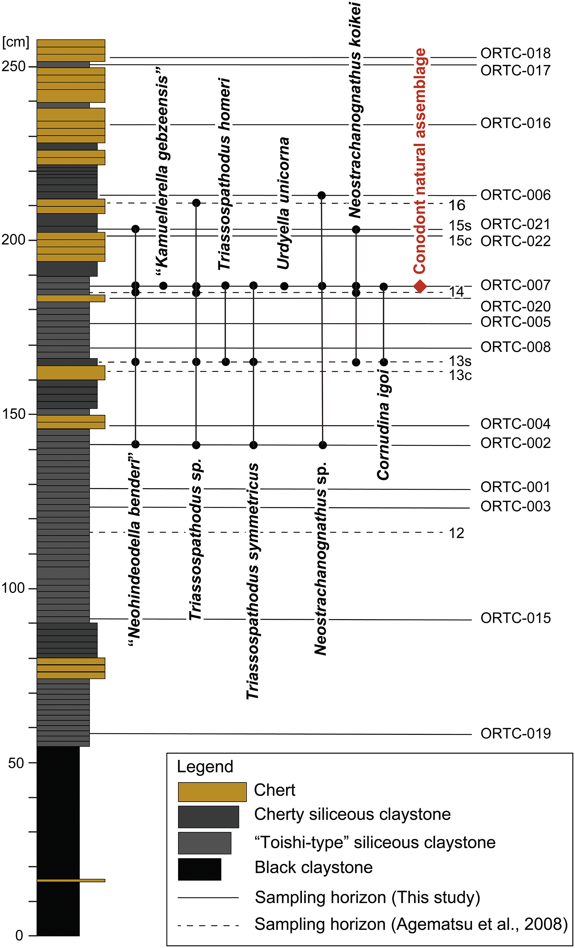
Figure 2. Long description
A vertical lithological column is scaled from 0 to 250 cm. The lithology from bottom to top consists of black claystone (0 to 55 cm), followed by alternating layers of Toishi-type siliceous claystone, cherty siliceous claystone, and chert.
To the right of the column, vertical lines represent the stratigraphic ranges of specific conodont species. From left to right, these include:
* Neohindeodella benderi: ranging from horizon O R T C-002 to O R T C-007.
* Kamuellerella gebzeensis: ranging from horizon O R T C-007 to O R T C-006.
* Triassospathodus sp.: ranging from horizon O R T C-002 to O R T C-006.
* Triassospathodus homeri: ranging from horizon 13s to O R T C-007.
* Triassospathodus symmetricus: ranging from horizon O R T C-002 to O R T C-007.
* Urdyella unicorna: ranging from horizon 13s to O R T C-007.
* Neostrachanognathus sp.: ranging from horizon O R T C-002 to O R T C-006.
* Neostrachanognathus koikei: ranging from horizon O R T C-007 to 15s.
* Cornudina igoi: ranging from horizon 13s to O R T C-007.
A red diamond at horizon O R T C-007 (approximately 185 cm) is labeled Conodont natural assemblage in red text.
Sampling horizons are marked by horizontal lines. Solid lines indicate this study (O R T C-019, 015, 003, 001, 002, 004, 008, 005, 020, 007, 022, 021, 006, 016, 017, 018). Dashed lines indicate Agematsu et al., 2008 (horizons 12, 13c, 13s, 14, 15c, 15s, 16).
The lower half of the “Toishi-type” siliceous claystone interval (55–120 cm above the base of the section) contains lenticular pyrite and is hard and weakly fissile. By contrast, the upper half (120–190 cm above the base of the section) is strongly fissile. Conodont elements are abundant in some layers. This lithofacies exhibits the diagnostic characters of “Toishi-type shale” (Imoto, Reference Imoto1984) and is the same as the lithofacies called “siliceous claystone” (e.g., Kakuwa, Reference Kakuwa1996, Reference Kakuwa2008; Isozaki, Reference Isozaki1997; Kamata, Reference Kamata1997, Reference Kamata, De Wever and Caulet1999; Sugiyama, Reference Sugiyama1997; Yamakita et al., Reference Yamakita, Kadota, Kato, Tada, Ogihara, Tajika and Hamada1999; Motoki and Sashida, Reference Motoki, Sashida and Sashida2004; Takahashi et al., Reference Takahashi, Yamakita, Suzuki, Kaiho and Ehiro2009a, Reference Takahashi, Oba, Kaiho, Yamakita and Sakatab; Muto et al., Reference Muto, Takahashi, Yamakita and Onoue2020), “siliceous shale” (e.g., Koike, Reference Koike1979; Sashida et al., Reference Sashida, Kamata and Igo1992; Sugiyama, Reference Sugiyama1992), “siliceous mudstone” (e.g., Yamakita, Reference Yamakita1987; Kuwahara et al., Reference Kuwahara, Nakae and Yao1991; Sakuma et al., Reference Sakuma, Tada, Ikeda, Kashiyama, Ohkouchi, Ogawa, Watanabe, Tajika and Yamamoto2012), “banded claystone” (e.g., Saito, Reference Saito1993; Saito et al., Reference Saito, Kimura, Naito and Sakai1996), “Toishi facies” (e.g., Wignall et al., Reference Wignal, Bond, Kuwahara, Kakuwa, Newton and Poulton2010), and “P–T boundary claystone” (e.g., Wakita and Metcalfe, Reference Wakita and Metcalfe2005). Furthermore, this lithofacies is similar to the “Type 1” “Toishi-type” siliceous claystone described by Motoki and Sashida (Reference Motoki, Sashida and Sashida2004).
The cherty siliceous claystone occurs 190–220 cm above the basement of the section. The claystone is black, dark gray, or gray in color, is weakly fissile, has a vitreous luster, and is commonly intercalated with chert layers a few centimeters thick. Bead-like spherical radiolarian tests are more abundant than in the “Toishi-type” siliceous claystone. The cherty siliceous claystone appears to be intermediate between the “Toishi-type” siliceous claystone and bedded chert. These features are consistent with those of “muddy chert” (e.g., Sugiyama, Reference Sugiyama1992; Muto et al., Reference Muto, Takahashi, Yamakita and Onoue2020), “black siliceous claystone” (Kamata, Reference Kamata, De Wever and Caulet1999), and “cherty siliceous claystone” (Muto et al., Reference Muto, Takahashi, Yamakita and Onoue2020) described previously. Moreover, this facies is comparable to the “Type 2” “Toishi-type” siliceous claystone defined by Motoki and Sashida (Reference Motoki, Sashida and Sashida2004). The bedded chert makes up the remaining parts of the section. The chert has a conspicuous vitreous luster, lacks fissility, and is black or dark gray in color. It comprises mainly microcrystalline to cryptocrystalline quartz and locally contains radiolarian tests. The thickness of each chert bed is 2–6 cm, and thin claystone layers occur between the chert beds. The transition from the “Toishi-type” siliceous claystone to the cherty siliceous claystone and then to the bedded chert is gradual.
Conodont fossils and age
In this work, the rock samples and fossil specimens studied by Agematsu et al. (Reference Agematsu, Orchard and Sashida2008) were reexamined, and 22 new rock samples were collected from the Oritachi section. The following conodont taxa were detected: P1 elements of Cornudina igoi Koike, Reference Koike, Noda and Sashida1996, Neostrachanognathus oezdemirae (Gedik, Reference Gedik1975), Neostrachanognathus koikei n. sp., Triassospathodus homeri (Bender, 1967), and Triassospathodus symmetricus (Orchard, Reference Orchard1995); S and M elements of Triassospathodus Kozur, Mostler, and Krainer, Reference Kozur, Mostler and Krainer1998 and Neostrachanognathus Koike, Reference Koike1998 (morphological identification based on Koike, Reference Koike2004; Orchard, Reference Orchard, Purnell and Donoghue2005; Agematsu et al., Reference Agematsu, Orchard and Sashida2008); Urdyella unicorna Leu and Goudemand in Leu et al. (Reference Leu, Bucher, Vennemann, Bagherpour, Ji, Brosse and Goudemand2022); “Neohindeodella benderi” (Kozur and Mostler, Reference Kozur and Mostler1970); and “Kamuellerella gebzeensis” Gedik, Reference Gedik1975 (Figs. 2, 3). In addition, one natural assemblage of N. koikei was found in a previously unexamined specimen from sample A of Agematsu et al. (Reference Agematsu, Orchard and Sashida2008), and two incomplete natural assemblage specimens were found in sample ORTC-007 (Figs. 2, 3).
Conodonts from the “Toishi-type” siliceous claystone in the Oritachi section. (1) Triassospathodus homeri (Bender, 1967), P1 element, IGUT-yf0004, sampling horizon 13s. (2–4) Triassospathodus symmetricus (Orchard, Reference Orchard1995), P1 element: (2) IGUT-yf0005, sampling horizon 13s; (3) IGUT-yf0006, sampling horizon ORTC-007; (4) IGUT-yf0007, sampling horizon ORTC-002. (5, 6) Cornudina igoi Koike, Reference Koike, Noda and Sashida1996, P1 element, sampling horizon ORTC-007: (5) IGUT-yf0008; (6) IGUT-yf0009. (7–10) Neostrachanognathus koikei n. sp.: (7) P1 element, IGUT-yf0010, sampling horizon 13s; (8) P1 element, IGUT-yf0011, sample A of Agematsu et al. (Reference Agematsu, Orchard and Sashida2008); (9) P2 element, IGUT-yf0012, sample A of Agematsu et al. (Reference Agematsu, Orchard and Sashida2008); (10) P2 element, IGUT-yf0013, sampling horizon 13s. (11) Urdyella unicorna Leu and Goudemand in Leu et al. (Reference Leu, Bucher, Vennemann, Bagherpour, Ji, Brosse and Goudemand2022), IGUT-yf0014, sampling horizon ORTC-007. (12, 13) “Neohindeodella benderi” (Kozur and Mostler, Reference Kozur and Mostler1970): (12) IGUT-yf0015, sampling horizon ORTC-002; (13) IGUT-yf0016, sampling horizon ORTC-007. (14) “Kamuellerella gebzeensis Gedik, Reference Gedik1975,” IGUT-yf0017, sampling horizon ORTC-007. (15) Natural assemblage of Neostrachanognathus koikei n. sp., holotype IGUT-yf0001, sample A of Agematsu et al. (Reference Agematsu, Orchard and Sashida2008). (16) Incomplete natural assemblage, IGUT-yf0002, sampling horizon ORTC-007. (17) Incomplete natural assemblage, IGUT-yf0003, sampling horizon ORTC-007. (1–15) Scale bars = 100 μm; (16, 17) scale bars = 200 μm. Rock samples are wetted and photographed under a stereomicroscope.
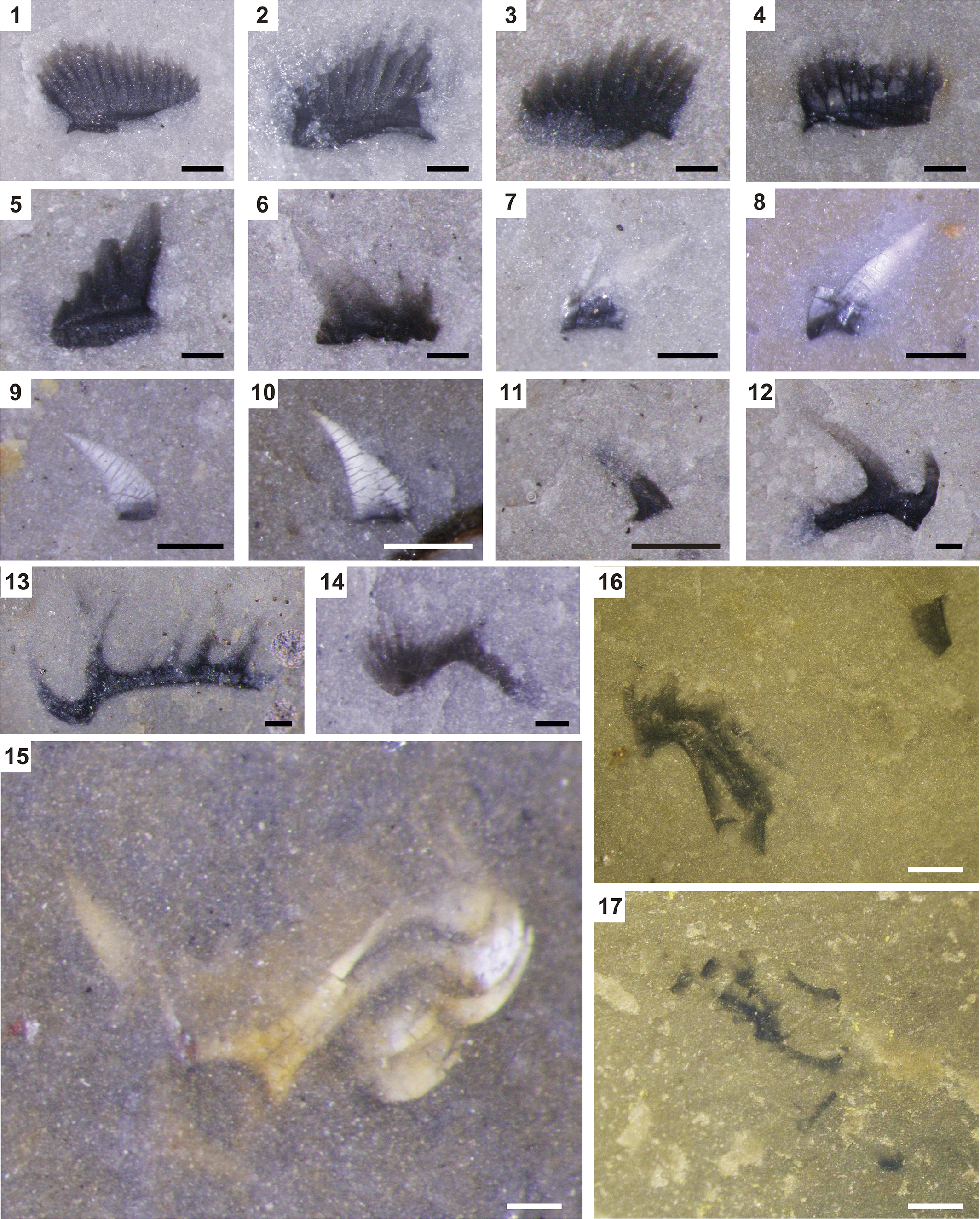
Figure 3. Long description
A collection of 17 microphotographs of conodont elements embedded in rock matrix.
* Panels 1 through 4 show Triassospathodus species P 1 elements, appearing as dark, fan-shaped or comb-like structures with multiple vertical denticles along a horizontal base.
* Panels 5 and 6 show Cornudina igoi P 1 elements, characterized by a prominent, tall central cusp and smaller flanking denticles.
* Panels 7 through 10 display Neostrachanognathus koikei elements. Panels 7 and 8 are P 1 elements with a triangular profile, while 9 and 10 are P 2 elements appearing as curved, elongated white structures.
* Panel 11 shows a small, dark Urdyella unicorna element.
* Panels 12 and 13 show Neohindeodella benderi, featuring long, curved processes with distinct spacing between denticles.
* Panel 14 shows a Kamuellerella gebzeensis element with a curved, arched base.
* Panel 15 is a larger view of a natural assemblage of Neostrachanognathus koikei, showing multiple elements clustered together in their original biological orientation.
* Panels 16 and 17 show incomplete natural assemblages, appearing as dark, fragmented clusters of elements against a lighter, yellowish-grey rock matrix.
Scale bars in panels 1 through 15 represent 100 micrometers. Scale bars in panels 16 and 17 represent 200 micrometers.
T. homeri and T. symmetricus have been reported worldwide, with a stratigraphic range from the lower Spathian to the Aegean (lowest Anisian, lower Middle Triassic) (e.g., Orchard, Reference Orchard2007, Reference Orchard and Lucas2010; Chen et al., Reference Chen, Jiang, Lai, Yan, Richoz, Liu and Wanga2015). N. oezdemirae occurs in the Aegean of the Kocaeli Peninsula in Turkey (Gedik, Reference Gedik1975; Kiliç, Reference Kiliç2021). Other Neostrachanognathus conodonts are known from Japan (e.g., Sashida et al., Reference Sashida, Kamata and Igo1992; Koike, Reference Koike1998; Agematsu et al., Reference Agematsu, Orchard and Sashida2008; Muto et al., Reference Muto, Takahashi, Yamakita, Soda and Onoue2019; Muto, Reference Muto2021; Ozeki et al., Reference Ozeki, Shimizu, Agematsu and Sashida2021), South China (Leu et al., Reference Leu, Bucher, Vennemann, Bagherpour, Ji, Brosse and Goudemand2022), the Russian Far East (as Cratognathodus sp.; Buryi, Reference Buryi1989), southern Thailand (Sashida and Igo, Reference Sashida and Igo1992; Tongtherm et al., Reference Tongtherm, Shigeta, Sardsud, Asato, Maekawa, Haga, Agematsu and Sashida2023), northern Malaysia (Koike, Reference Koike, Kobayashi, Toriyama and Hashimoto1982), Turkey (Gedik, Reference Gedik1975; Kiliç et al., Reference Kiliç, Plasencia and Önder2018; Kiliç, Reference Kiliç2021), Oman (Agematsu et al., Reference Agematsu, Orchard and Sashida2008; Chen et al., Reference Chen, Richoz, Krystyn and Zhang2019; Leu et al., Reference Leu, Bucher, Baud, Vennemann, Luz, Hautmann and Goudemand2023), and New Zealand (Hori et al., Reference Hori, Yamakita, Ikehara, Kodamac and Aita2011), and generally range from lower Spathian to Aegean (Koike, Reference Koike1998). P1 elements of Neostrachanognathus, together with the Middle Triassic radiolarian Eptingium Manfredi Dumitrica, Reference Dumitrica1978, have been found in siliceous mudstone pebbles in conglomerates from the Cretaceous Sanchu Group in Japan, suggesting that the range of this genus may extend from the middle Anisian to the earliest Ladinian (Ozeki et al., Reference Ozeki, Shimizu, Agematsu and Sashida2021). “Neohindeodella benderi” is characterized by a bipennate ramiform element with a strong downward-arching curvature and an elongated anterior-end denticle and cusp. In this study, while we assume this form represents the S elements of N. tahoensis as described in the Systematic paleonotology, the multi-element taxonomy remains undetermined. However, “N. benderi” is used as a biostratigraphic marker because of its abundance in “Toishi-type” siliceous claystone and its easily recognizable morphology. It is considered to indicate a late Spathian to Aegean age (e.g., Koike, Reference Koike1979; Takahashi et al., Reference Takahashi, Oba, Kaiho, Yamakita and Sakata2009b). U. unicorna is an elongated conical form found in middle Smithian (lower Olenekian, upper Lower Triassic) to lower upper Smithian strata of South China and Spathian rocks in India, Oman, and North America (Leu et al., Reference Leu, Bucher, Vennemann, Bagherpour, Ji, Brosse and Goudemand2022).
Judging from these conodont fossils, the depositional age of the “Toishi-type” siliceous claystone comprising the Oritachi section is estimated to be middle Spathian to early Aegean. This conclusion is consistent with the ages of other “Toishi-type” siliceous claystone sections in Japan (e.g., Koike, Reference Koike1979; Tanaka, Reference Tanaka1980; Sashida et al., Reference Sashida, Kamata and Igo1992; Takahashi et al., Reference Takahashi, Oba, Kaiho, Yamakita and Sakata2009b; Muto et al., Reference Muto, Takahashi, Yamakita, Suzuki, Suzuki and Aita2018, Reference Muto, Takahashi, Yamakita, Soda and Onoue2019; Muto, Reference Muto2021).
Conodont apparatus of Neostrachanognathus
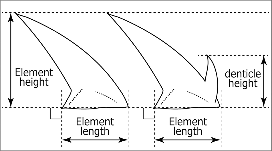
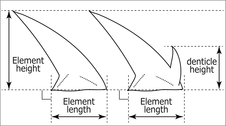
A three-dimensional model of the conodont assemblage of Neostrachanognathus and the element organization are shown in Figures 4, 5. The natural assemblage measures 800 μm along the rostro-caudal axis and 600 μm along the dorso-ventral axis on the stratigraphic plane and is strongly compacted in the sinistro-dextral axial direction to a thickness of ~200 μm. Analysis using ImageJ, Drishti, and Avizo was performed to identify the dextral S-element group, sinistral S-element group, M-element group, and P-element group from the rostral to the caudal side of the assemblage specimen. The conical P1 elements have a robust base and tapered cusp with an arched anterior margin. In the Avizo image, although the central area of the sinistral P1 element appears to be missing (Fig. 5), almost the entire cusp can be observed under a stereomicroscope (Fig. 5.4), which suggests that this “absence” is due to the characteristics of X-ray imaging (Agematsu et al., Reference Agematsu, Fukushima, Fujisaki and Ozeki2024). The antero-posteriorly short basal cavity visible in the Avizo image indicates that the postero-basal corner of the base is not elongated (Fig. 5). The existence of the antero-lateral denticle is unclear in both dextral and sinistral P1, but a denticle that is half the length of the cusp may be visible in sinistral P1 under a stereomicroscope (Fig. 5.4). The P2 elements also have a conical form similar to P1. As with P1, due to the properties of X-ray imaging, only the basal outlines of both P2 elements and the tip of the sinistral one can be identified in the Avizo image (Fig. 5). However, the element profile on the tomographic image shows there are no antero-lateral denticles. The height/length ratio (Fig. 6) of P1 is 1.6 and that of P2 is 1.7. From these morphological features, these four P elements are identified as Neostrachanognathus koikei n. sp.
Three-dimensional model constructed by Drishti, conodont assemblage of Neostrachanognathus koikei n. sp., holotype IGUT-yf0001 from the “Toishi-type” siliceous claystone, sample A, the Oritachi section. (1) Dextral view. (2) Colored on (1). P1-2d, Md, and S1-4d are dextral elements; P1-2s, Ms, and S1-4s are sinistral elements.
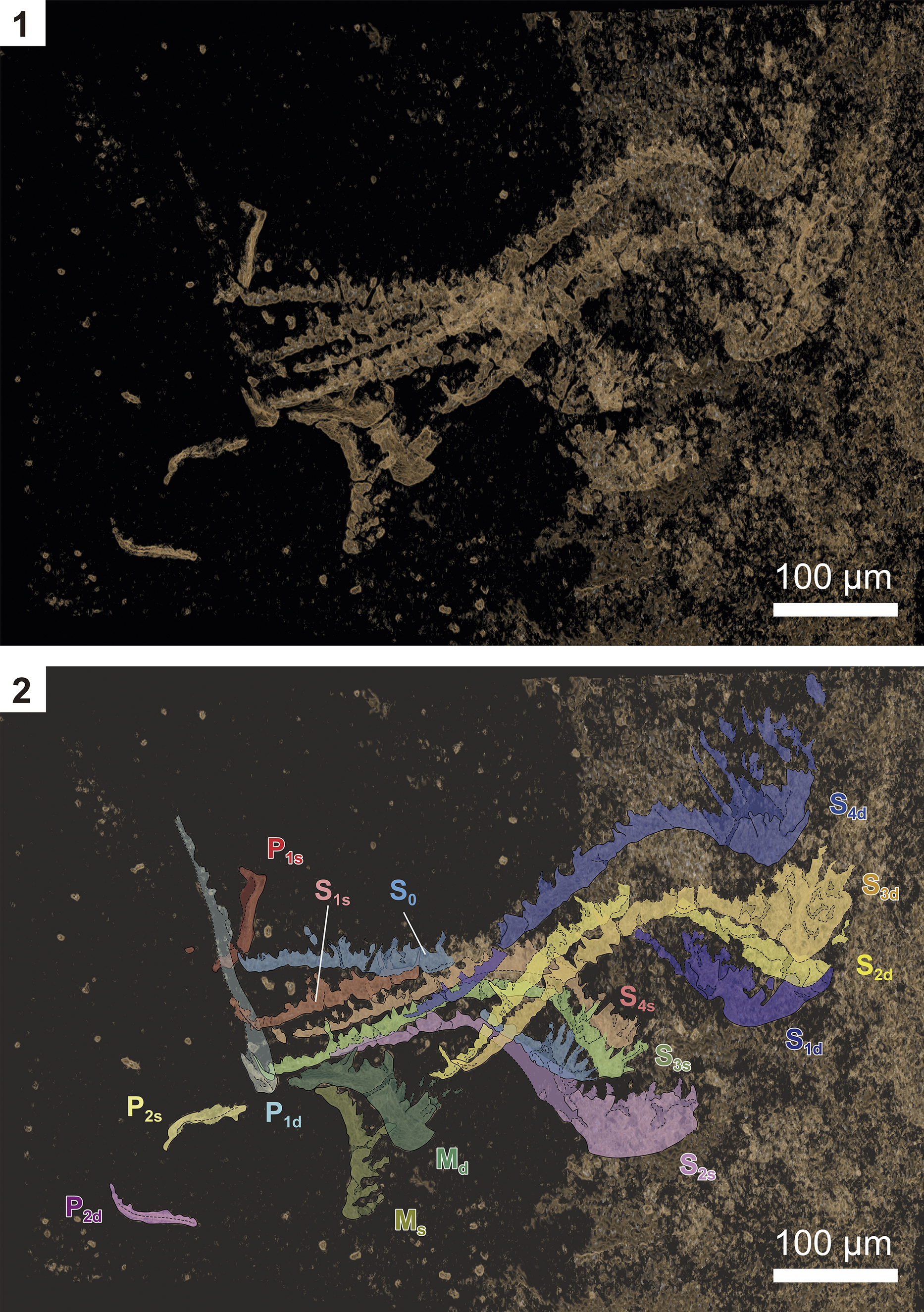
Figure 4. Long description
A two-panel vertical layout showing a fossilized conodont assemblage of Neostrachanognathus koikei n. sp. Both panels include a 100 micrometer scale bar in the bottom right corner.
Panel 1: A dextral view of the three-dimensional model against a dark background. The fossil elements appear as tan, elongated, and serrated structures clustered together, with some fragments scattered to the left.
Panel 2: The same view as panel 1 but with individual elements highlighted in different colors and labeled with alphanumeric codes.
* P elements: P 1 s is red, P 1 d is light blue, P 2 s is yellow-green, and P 2 d is pink. These are located on the left side of the cluster.
* M elements: M d is dark green and M s is light green, positioned at the bottom center of the assemblage.
* S elements: S 0 is light blue at the center. S 1 s is brown, S 1 d is dark blue, S 2 s is purple, S 2 d is yellow, S 3 s is light green, S 3 d is tan, S 4 s is pinkish-brown, and S 4 d is medium blue. These elements form the elongated, curved, and serrated tail-like structures extending toward the right side of the frame.
Three-dimensional model constructed by Avizo, conodont assemblage of Neostrachanognathus koikei n. sp., holotype IGUT-yf0001 from the “Toishi-type” siliceous claystone, sample A, the Oritachi section. (1) Dextral view. (2) Sinistral view. (3) Caudal view. (4) Stereomicroscopic photographs and line drawings of element outline. P1-2d, Md, and S1-4d are dextral elements, P1-2s, Ms, and S1-4s are sinistral elements. Colors of the letters correspond to Figure 4.2.
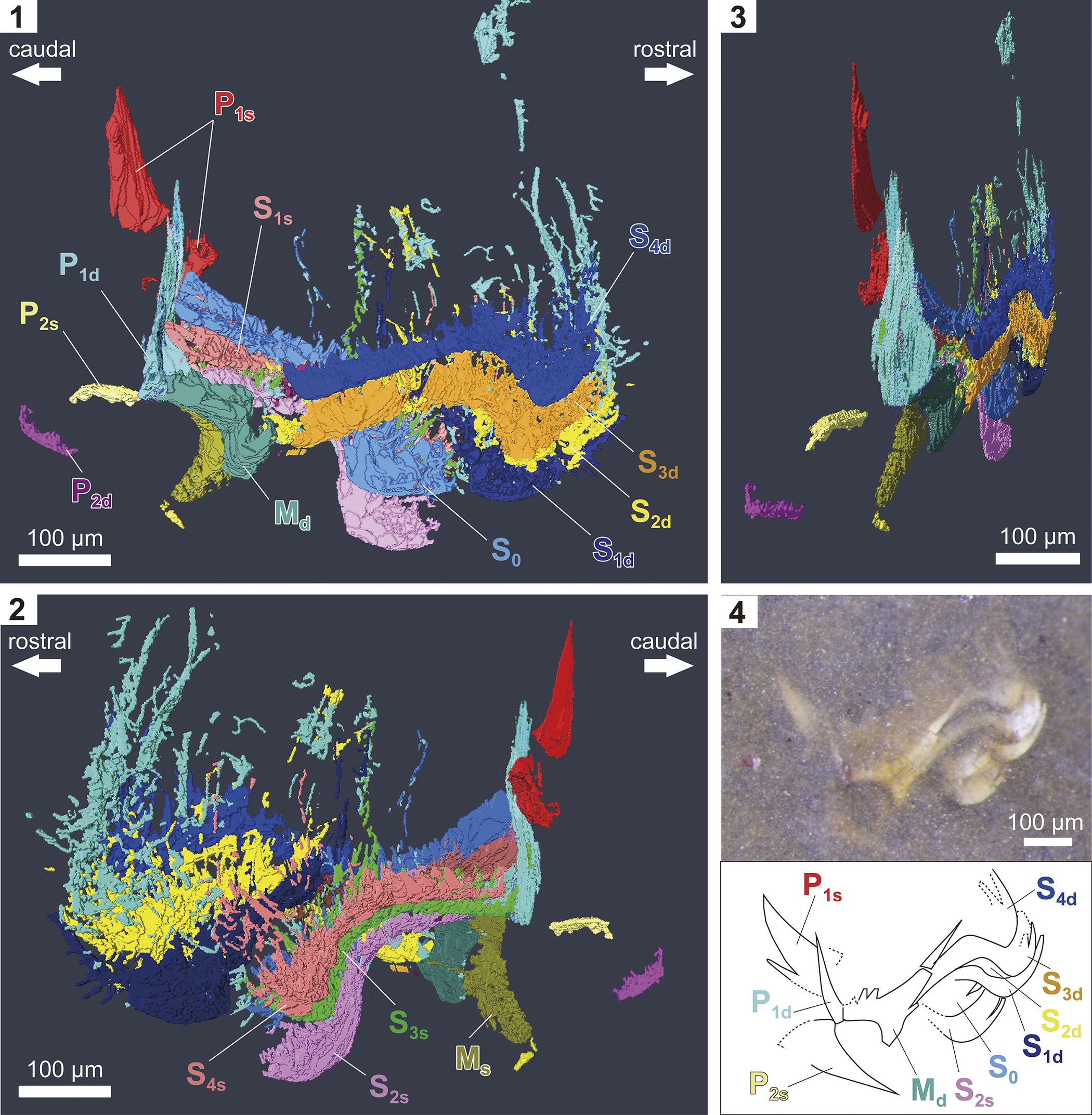
Figure 5. Long description
A multi-panel scientific visualization of a conodont holotype.
Panel 1: Dextral view of a 3 D reconstruction. A scale bar indicates 100 micrometers. Arrows at the top point left for caudal and right for rostral. Labeled elements include P 1 s in red, P 1 d in light blue, P 2 s in yellow, P 2 d in pink, M d in olive green, S 1 s in light pink, S 0 in light purple, S 1 d in dark blue, S 2 d in yellow, S 3 d in orange, and S 4 d in medium blue. The elements form a complex, interlocking cluster.
Panel 2: Sinistral view of the same 3 D model. Arrows at the top point left for rostral and right for caudal. Labeled elements include S 4 s in teal, S 3 s in green, S 2 s in purple, and M s in olive green. The cluster shows a dense arrangement of elongated, curved structures.
Panel 3: Caudal view of the 3 D model showing the vertical and lateral distribution of the elements. A 100 micrometer scale bar is at the bottom right.
Panel 4: Top half contains a stereomicroscopic photograph of the fossil specimen in matrix with a 100 micrometer scale bar. Bottom half contains a line drawing of the element outlines with corresponding labels: P 1 s, P 1 d, P 2 s, M d, S 2 s, S 0, S 1 d, S 2 d, S 3 d, and S 4 d. The lines trace the sharp, blade-like and needle-like morphology of the individual conodont elements.
Lengths and heights of elements measured in this study.
Reconstruction of the conodont apparatus composition of Neostrachanognathus based on this specimen is shown in Figure 7. The S position consists of four pairs on each side (S1 to S4) and a single S0 position in the center. The elements occupying these places have almost identical morphology, although in this specimen they are compressed laterally and quite flattened. Unlike many ellisonids and gondolelloids, the conodonts of this genus have S0 elements without a branched anterior process and S1–S4 elements with undifferentiated morphology. It is likely that S0 elements could not be recognized in the previously reported Neostrachanognathus assemblages because they are indistinguishable in morphology from the S1–S4 elements. In addition, a pair of elements is placed in the position designated as M in this paper, which corresponds to P3 of Agematsu et al. (Reference Agematsu, Orchard and Sashida2008). Although this position is much more caudal than the commonly known M position of an ozarkodinid-type apparatus, given the homology of the elements it is more reasonable to consider that the M pair underwent an evolutionary shift to a caudal direction rather than to assume this is the third P pair. In summary, Neostrachanognathus conodonts have an apparatus consisting of nine S, two M, and four P elements.
Reconstructed components of the apparatus of Neostrachanognathus koikei n. sp. (1) General morphology of the eight types of elements. (2) Rostral view of the architecture. (3) Caudal view of the architecture. Apparatus reconstruction modified from Agematsu et al. (Reference Agematsu, Orchard and Sashida2008).
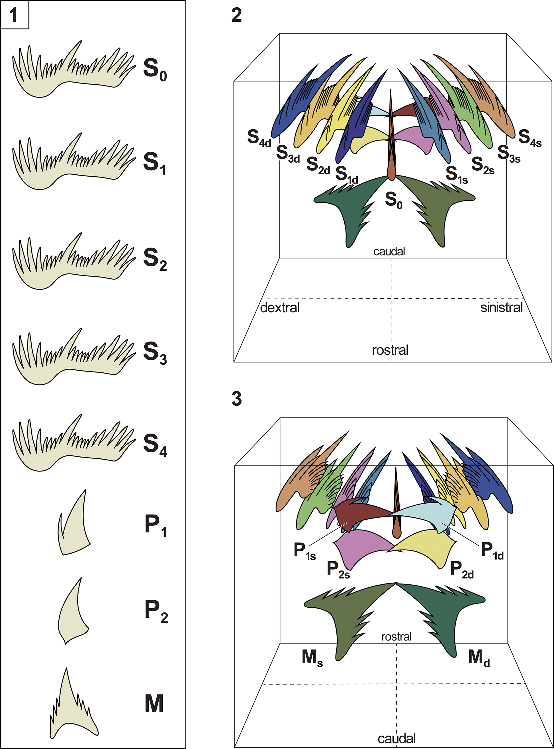
Figure 7. Long description
The diagram consists of three panels.
Panel 1 is a vertical column displaying eight distinct element types of the apparatus. From top to bottom, they are labeled S sub 0, S sub 1, S sub 2, S sub 3, and S sub 4, which are comb-like elongated elements with multiple denticles. Below these are P sub 1 and P sub 2, which are simpler, blade-like elements, and M, a broad, triangular element with a serrated base.
Panel 2 shows a rostral view of the reconstructed architecture within a transparent cube. At the center is the S sub 0 element. Arranged symmetrically on either side are the S sub 1, S sub 2, S sub 3, and S sub 4 elements, labeled with ‘d’ for dextral (right) and ‘s’ for sinistral (left). The elements are color-coded: S sub 1 is blue, S sub 2 is yellow, S sub 3 is purple, and S sub 4 is orange. The floor of the cube is marked with axes for dextral, sinistral, rostral, and caudal directions.
Panel 3 shows a caudal view of the architecture. It highlights the positioning of the P and M elements. The M sub s and M sub d elements are large, dark green structures at the base. Above them are the P sub 2 and P sub 1 elements, shown in pink, yellow, and light blue. The S elements are visible in the background, maintaining the same color-coding as Panel 2. The orientation of the rostral and caudal axes on the floor is reversed compared to Panel 2.
Discussion
Phylogenic relationships
In this paper, the apparatus of Neostrachanognathus Koike, Reference Koike1998 is restored as a bilaterally symmetrical organ composed of 15 elements corresponding to those of typical ozarkodinids, arranged in pairs of P1, P2, M, S1, S2, S3, and S4 and a single S0 element. Unlike most Triassic conodonts, this apparatus shows convergent element morphology and low diversity of S elements. The P1 and P2 elements have a conical form in which a prominent cusp is the main unit. The S elements are bipennate ramiforms, with little difference in their morphology, characterized especially by the S0 element not being an alate form.
The superfamily Gondolelloidea and family Ellisoniidae, to which most Early Triassic conodonts belong, had an apparatus consisting of 15 elements (Orchard and Rieber, Reference Orchard and Rieber1999; Koike et al., Reference Koike, Yamakita and Kadota2004; Orchard, Reference Orchard, Purnell and Donoghue2005; Koike, Reference Koike2016). As mentioned, “atavistic” conical forms are known to occur in the Early Triassic. Currently, conodonts with these morphologies are generally included in the subfamily Cornudininae (Orchard, Reference Orchard, Purnell and Donoghue2005, Reference Orchard2007); for example, the P1 elements of Cornudina Hirschmann, Reference Hirschmann1959 and Spathicuspus Orchard, Reference Orchard, Purnell and Donoghue2005 are short segminate pectiniforms with a prominent cusp. Leu et al. (Reference Leu, Bucher, Vennemann, Bagherpour, Ji, Brosse and Goudemand2022) recently described other elements showing a conical form as Urdyella Leu and Goudemand in Leu et al., Reference Leu, Bucher, Vennemann, Bagherpour, Ji, Brosse and Goudemand2022 and placed that genus in the Cornudininae. However, it is not clear what apparatuses these conical elements were part of. The conodont apparatus of the Cornudininae, part of the Gondolelloidea, consists of 15 types of elements (Orchard, Reference Orchard, Purnell and Donoghue2005): segminate or segminiplanate P1 elements; angulate P2 elements; breviform digyrate M elements; an alate S0 element; breviform digyrate ramiform S1 elements; digyrate ramiform S2 elements; and bipennate ramiform S3–4 elements.
Much remains unknown about the ellisonid conodonts. Sweet (Reference Sweet, Kummel and Teichert1970) and Koike (Reference Koike1990) estimated the apparatus of Ellisonia triassica Müller, Reference Müller1956, the type species of Ellisonia Müller, Reference Müller1956, representing the Ellisoniidae, but did not address the P1 element. Orchard (Reference Orchard2007) noted this point, stating that small segminate or angulate elements, such as the Griesbachian species Merrillina?/Ellisonia? peculiaris (Sweet, Reference Sweet, Kummel and Teichert1970), are likely to represent the P elements of Ellisonia. Koike (Reference Koike2016) attempted apparatus reconstruction for the Smithian E. triassica based on the natural assemblage of Ellisonia sp. cf. E. triassica described by Koike et al. (Reference Koike2004) from uppermost Permian strata in Japan; the frequent association of ellisonid elements from the Lower Triassic Taho Formation, Japan; and the hypothesis of Sweet (Reference Sweet1988). Koike (Reference Koike2016) concluded that this species possesses angulate, palmate, pastinate, or pastiniplanate P1 elements; angulate or palmate P2 elements; breviform digyrate M elements; an alate S0 element; extensiform digyrate S1 and S2 elements; and bipennate S3 and S4 elements.
Neostrachanognathus lacks an “enantiognathiform” S1 element, a diagnostic feature of the Gondolelloidea (Orchard, Reference Orchard, Purnell and Donoghue2005) and is therefore excluded from this group. Furthermore, because the S0 element does not branch and the S1–S4 elements share the same morphology, it is difficult to directly compare Neostrachanognathus with ellisonids. However, the S elements of Neostrachanognathus are identified as some form of a Triassic form genus “Neohindeodella” Kozur, Reference Kozur1968. As explained in the section Neostrachanognathus and “Neohindeodella” below, the synonyms of Ellisonia include “Neohindeodella,” and some forms of “Neohindeodella” are assigned to S elements of the multi-element species E. triassica (Sweet, Reference Sweet, Kummel and Teichert1970). In other words, the S elements of Neostrachanognathus share diagnostic characters with the S elements of some species within the Ellisoniidae. Therefore, this paper concludes that Neostrachanognathus represents a group that diverged from the Ellisonia lineage during the Early Triassic with a simplification of element morphology. The ancestor of Neostrachanognathus may have been the Griesbachian M?/E? peculiaris (Sweet, Reference Sweet, Kummel and Teichert1970).
Kiliç et al. (Reference Kiliç, Plasencia and Önder2018) discussed the element composition and relationships of the subfamily Cornudinae and the Gondolellidae using specimens of “Cornudina” from Turkey. He proposed an element composition with “Cornudina” as the P elements, the form genus “Ketinella” Gedik, Reference Gedik1975 as the M elements, and the form genus “Kamuellerella” Gedik, Reference Gedik1975 as the S elements. However, it appears that at least some of the Cornudina elements discussed by Kiliç et al. (Reference Kiliç, Plasencia and Önder2018) are components of Neostrachanognathus, which includes Neostrachanognathus oezdemirae (Gedik, Reference Gedik1975) (= Cornudina oezdemirae of Kiliç et al., Reference Kiliç, Plasencia and Önder2018: P elements), “Ketinella” (M elements), and “Kamuellerella” (S elements). Note that the problem highlighted by Kiliç et al. (Reference Kiliç, Plasencia and Önder2018) regarding the coexistence of Cornudina, “Ketinella,” and “Kamuellerella” elements is not likely to be a major issue because all three genera are known to co-occur, at least, in a pelagic siliceous rock sequence in Japan (e.g., Muto et al., Reference Muto, Takahashi, Yamakita, Soda and Onoue2019).
Orchard (Reference Orchard2007) postulated an evolutionary trend in Early Triassic coniform conodonts toward a reduction or loss of anterior processes in the segminate pectiniforms and proposed a divergence from Neospathodus Mosher, Reference Mosher1968, with a relatively prominent cusp (e.g., Neospathodus chii Zhao and Orchard in Zhao et al., Reference Zhao, Orchard, Tong, Sun, Zuo, Zhang and Yun2007), to Spathicuspus, Cornudina, and Neostrachanognathus. This evolutionary trend toward a more prominent cusp and fewer denticles has also been observed in the upper Wuchiapingian–lower Changhsingian genus Merrillina Kozur, Reference Kozur1975 (Wang et al., Reference Wang, Sun, Wignall, Xing, Chen and Lai2023). Merrillina is considered to be directly related to the Triassic Ellisonia (Kozur, Reference Kozur2004), and as mentioned, it has been suggested that conodonts with small elements such as M?/E? peculiaris may have originated during the Griesbachian (Orchard, Reference Orchard2007). Although it remains unclear whether M?/E? peculiaris was the ancestor of Neostrachanognathus, this “simplification” of element morphology appears to have been an evolutionary trend in both the ellisonid and gondolleloid lineages from the late Permian into the Early Triassic. The P elements of Neostrachanognathus tahoensis (“true” tahoensis of Koike, Reference Koike1998), which have a stratigraphic range of Smithian to lower Spathian, are characterized by multiple denticles in the antero-lateral process, posterior denticles, and posterobasal corners that strongly project posteriorly (wide basal cavity). By contrast, N. koikei n. sp. (lower Spathian to Aegean) and N. oezdemirae (lower Spathian to Aegean) have one to two anterior denticles and a shortened posterobasal corner (narrower basal cavity). Thus, the anterior and posterior denticles became reduced during the evolutionary sequence from N. tahoensis to N. koikei and N. oezdemirae (Fig. 8).
Stratigraphic ranges and element morphology of Neostrachanognathus koikei n. sp., Neostrachanognathus tahoensis Koike, Reference Koike1998, Neostrachanognathus oezdemirae (Gedik, Reference Gedik1975), Spathicuspus spathi (Sweet, Reference Sweet, Kummel and Teichert1970), and Cornudina igoi Koike, Reference Koike, Noda and Sashida1996. Drawings of the elements of N. tahoensis are based on Koike (Reference Koike1998) and Agematsu et al. (Reference Agematsu, Orchard and Sashida2008); P1 element of N. oezdemirae is based on Gedik (Reference Gedik1975); M and S elements of N. oezdemirae are based on “Ketinella” and “Kamuellerella” of Gedik (Reference Gedik1975) and Kiliç et al. (Reference Kiliç, Plasencia and Önder2018). P1 element of S. spathi is based on Sweet (Reference Sweet, Kummel and Teichert1970); P1 element of C. igoi is based on Koike (Reference Koike, Noda and Sashida1996). Geologic age follows Ogg and Chen (Reference Ogg, Chen, Gradstein, Ogg, Schmitz and Ogg2020). Bi. = Bithynian.
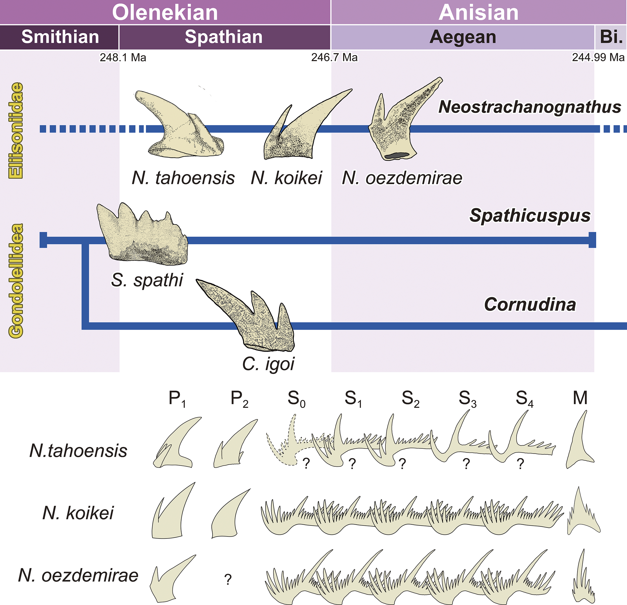
Figure 8. Long description
A stratigraphic diagram divided into two main sections.
Top section: A timeline spanning the Olenekian (Smithian and Spathian stages) and Anisian (Aegean and Bithynian stages) from 248.1 M a to 244.99 M a. Below the timeline, two horizontal blue lineages represent Ellisoniidae and Gondolellidae.
* The Ellisoniidae lineage includes Neostrachanognathus tahoensis (Spathian), N. koikei (late Spathian), and N. oezdemirae (Aegean).
* The Gondolellidae lineage branches into Spathicuspus spathi and Cornudina igoi during the Spathian.
Bottom section: A morphological grid comparing elements labeled P sub 1, P sub 2, S sub 0, S sub 1, S sub 2, S sub 3, S sub 4, and M for three species.
* N. tahoensis: Features simple, curved P elements and complex, multi-denticulated S elements, some marked with question marks.
* N. koikei: Shows broader P elements and highly serrated, comb-like S elements.
* N. oezdemirae: Displays slender, elongated P sub 1 elements, a question mark for P sub 2, and deeply branched S elements with prominent primary cusps.
Neostrachanognathus and “Neohindeodella.”—Kozur (Reference Kozur1968) described conodonts from the upper Muschelkalk of the Germanic Basin and first described “Neohindeodella” as a subgenus of “Hindeodella” Ulrich and Bassler, Reference Ulriche and Bassler1926. Subsequently elevated to genus, “Neohindeodella” is distinguished from other groups by its high, short processes bearing numerous denticles, which often reach their maximum size at the anterior and posterior ends of the processes; the attachment surface at the base being “inverted”; and the absence of a basal groove and basal pit (e.g., Kozur, Reference Kozur1968; Kozur and Mostler, Reference Kozur and Mostler1970, Reference Kozur and Mostler1972). By 1995, 17 species had been described, including the type species “Neohindeodella triassica” (Müller, Reference Müller1956), “Neohindeodella aequiramosa” Kozur and Mostler, Reference Kozur and Mostler1970, “Neohindeodella benderi,” “Neohindeodella nevadensis” (Müller, Reference Müller1956), and “Neohindeodella raridenticulata” (Müller, Reference Müller1956) (e.g., Kozur and Mostler, Reference Kozur and Mostler1970, Reference Kozur and Mostler1972; Wang, Reference Wang1978; Kozur and Mock, Reference Kozur and Mock1991; Götz, Reference Götz1995). However, Sweet (Reference Sweet, Kummel and Teichert1970) described conodonts from upper Permian to Lower Triassic strata of West Pakistan and assigned “Neohindeodella” as a synonym of the multi-element genus Ellisonia. At that time, “Nh. nevadensis,” “Nh. triassica,” and “Nh. raridenticulata” were chosen as the S2 element (LB element in Sweet, Reference Sweet, Kummel and Teichert1970) for the type species of Ellisonia, E. triassica (Sweet, Reference Sweet, Kummel and Teichert1970; Koike, Reference Koike1990). The type species of “Neohindeodella,” “Nh. triassica,” became a synonym of E. triassica, leading to the gradual discontinuation of “Neohindeodella.” However, some species remain widely recognized as form species because they are still valid as index fossils. In particular, “Nh. aequiramosa” and “Nh. benderi” are frequently found and reported from Lower Triassic “Toishi-type” siliceous claystones in Japan (e.g., Sashida et al., Reference Sashida, Kamata and Igo1992; Muto et al., Reference Muto, Takahashi, Yamakita, Suzuki, Suzuki and Aita2018, Reference Muto, Takahashi, Yamakita, Soda and Onoue2019). This section discusses the identification of some “Nh. aequiramosa” as N. koikei and the possibility of “Nh. benderi” being the S element of N. tahoensis.
The typical morphology of “Nh. aequiramosa” features anterior and posterior processes of nearly equal length, sometimes with the anterior one longer; the three to four denticles at the anterior end of the anterior process are large, often longer than a cusp; the three to five posterior denticles at the posterior end of the posterior process are large; and the basal line of the anterior process, viewed laterally, points downward in its posterior third (Kozur and Mostler, Reference Kozur and Mostler1970). The S element of N. koikei exhibits a bipennate, “neohindeodelliform” morphology. Its relatively long anterior process bears large denticles at the anterior end, which are as long as a cusp, resembling those of “Nh. aequiramosa”. However, these elements tend to have posterior processes that are somewhat longer than the anterior ones, and the basal line of the anterior process appears straight in lateral view, lacking the curvature at the one-third point. Consequently, the morphology of N. koikei S elements differs from that of typical specimens, including the holotype of “Nh. aequiramosa.” Morphology of the holotype of “Nh. aequiramosa” has a stratigraphic range from the Pelsonian (middle Anisian) to the Norian (Late Triassic) (e.g., Budurov, Reference Budurov1960; Kozur and Mostler, Reference Kozur and Mostler1970; Koike, Reference Koike1981). Forms comparable to the S element of N. koikei range from the Spathian to the lower Anisian, coinciding with the stratigraphic distribution of the P elements of N. koikei. Therefore, the S element of N. koikei can be identified as belonging to the Spathian and Anisian forms previously identified as “Nh. aequiramosa.”
As pointed out by Muto et al. (Reference Muto, Takahashi, Yamakita and Onoue2020), the P1 element of Neostrachanognathus sp. A described by Agematsu et al. (Reference Agematsu, Orchard and Sashida2008) can be identified as belonging to N. tahoensis (true tahoensis) (Agematsu et al., Reference Agematsu, Orchard and Sashida2008, text-fig. 8A–F). Among these elements, the P1 form (Agematsu et al., Reference Agematsu, Orchard and Sashida2008, text-fig. 8A–C) features a posterior process extending from a large cusp, likely bearing one denticle, and an antero-lateral corner projecting significantly, accompanied by two or three denticles. The P2 form (Agematsu et al., Reference Agematsu, Orchard and Sashida2008, text-fig. 8D–F) is similar to the P1 of N. koikei but differs from N. koikei in that the antero-lateral corner projects distinctly onto the lateral side. These Neostrachanognathus sp. A specimens were contained within rock samples collected from a single outcrop in Oman and are considered to be closely related to each other (Agematsu et al., Reference Agematsu, Orchard and Sashida2008). Therefore, this set of elements is likely to be a constituent of the apparatus of N. tahoensis. The S elements of Neostrachanognathus sp. A (Agematsu et al., Reference Agematsu, Orchard and Sashida2008, text-fig. 8I–K) have a short anterior process bearing a single large anterior-end denticle and often several relatively short denticles and are compared with “Nh. benderi.” The S elements of Neostrachanognathus sp. A include those lacking a denticle between the anterior-end denticle and the cusp (Agematsu et al., Reference Agematsu, Orchard and Sashida2008, fig. 8I), one denticle (Agematsu et al., Reference Agematsu, Orchard and Sashida2008, fig. 8K), and two denticles (Agematsu et al., Reference Agematsu, Orchard and Sashida2008, fig. 8J). These slightly different morphologies could potentially be placed at any position from S0 to S4 within a single apparatus. Among the “Kamuellerella” species proposed by Kiliç et al. (Reference Kiliç, Plasencia and Önder2018) as S elements of “Cornudia (here referred to as Neostrachanognathus), “Kamuellerella gebzeensis Gedik, Reference Gedik1975” may be identified as an S element of N. oezdemirae. This form resembles the S element of N. koikei but is distinguished from N. koikei by its shorter and lower posterior processes compared with the anterior processes. Muto et al. (Reference Muto, Takahashi, Yamakita and Onoue2020) and Muto (Reference Muto2021) reassigned “K. gebzeensis” to “Neohindeodella,” and these taxa appear to be closely related.
To date, N. koikei has been reported from sedimentary rocks formed in shallow water on a continental shelf (e.g., South China and Thailand) and in open-ocean environments (e.g., Japan and Russian Far East) (e.g., Buryi, Reference Buryi1989; Sashida et al., Reference Sashida, Kamata and Igo1992; Koike, Reference Koike1998; Leu et al., Reference Leu, Bucher, Vennemann, Bagherpour, Ji, Brosse and Goudemand2022). Neostrachanognathus must have been a group that expanded its distribution worldwide and thrived from the late Early Triassic to the early Middle Triassic.
Conclusion
Judging from natural assemblages of the Early Triassic conodont Neostrachanognathus koikei n. sp., we make the following conclusions. (1) The conodont apparatus of Neostrachanognathus consists of 15 elements occupying two pairs of P positions, one pair of M positions, four pairs of S positions, and a single S0 position. The P1 and P2 elements are conical forms; the nine S elements are similar in form to each other and are difficult to distinguish. (2) The S elements of Neostrachanognathus can be identified in some forms of “Neohindeodella aequiramosa.” From this relationship, we conclude that Neostrachanognathus derived from the family Ellisoniidae. (3) The S elements of Neostrachanognathus tahoensis are likely identifiable as “Neohindeodella benderi.” (4) During the Early Triassic, an evolutionary trend toward reduced denticles and processes on P elements occurred within both the Ellisoniidae and Gondolleloidea lineages. Among these, Neostrachanognathus was a taxon showing particularly marked simplification not only in P elements but also in the morphological diversity of S elements.
Systematic paleontology
The conodont description was carried out by Y.F. and S.A. The orientations of elements in the conodont apparatus and the nomenclature based on multi-element taxonomy are based on Purnell et al. (Reference Purnell, Donoghue and Aldridge2000). The general morphological scheme of conodont elements follows that of Sweet (Reference Sweet1988), and the morphological terminology of the genus Neostrachanognathus is based on Koike (Reference Koike1998) and Agematsu et al. (Reference Agematsu, Orchard and Sashida2008). Supergeneric classification of conodonts mostly follows that of Fåhraeus (Reference Fåhraeus1983), Orchard (Reference Orchard, Purnell and Donoghue2005), and Donoghue et al. (Reference Donoghue, Purnell, Aldridge and Zhang2008).
Class Conodonta Pander, Reference Pander1856
Order Ozarkodinida Dzik, Reference Dzik1976
Family Ellisoniidae Clark, Reference Clark, Lindström and Ziegler1972
Genus Neostrachanognathus Koike, Reference Koike1998
Type species
Neostrachanognathus tahoensis Koike, Reference Koike1998 (YNUC15876) from the Taho Limestone, Tahokamigumi, Shirokawa-cho, Seiyo City, Ehime Prefecture, Japan, by original designation.
Other species
N. oezdemirae (Gedik, Reference Gedik1975), N. sp. A of Agematsu et al. (Reference Agematsu, Orchard and Sashida2008), N. sp. A of Leu and Goudemand in Leu et al. (Reference Leu, Bucher, Vennemann, Bagherpour, Ji, Brosse and Goudemand2022), and N. koikei n. sp.
Diagnosis
Neostrachanognathus conodont has a bilaterally symmetrical apparatus consisting of 15 elements arranged in paired P1, P2, M, S1, S2, S3, and S4 positions and a single S0 position. The P1 and P2 elements are conical in form and may be accompanied by one or more denticles with a prominent cusp as a main unit. The S elements are bipennate, neohindeodelliform, and closely resemble each other; in particular, the S0 element is characterized by a non-alate ramiform. The M elements are breviform digyrate.
Occurrence
This genus has been reported from Smithian (upper Lower Triassic)–Aegean (lowest Anisian, Middle Triassic) strata in Kumamoto, Oita, Ehime, Kyoto, Aichi, and Gumma and Tochigi prefectures, Japan (Sashida et al., Reference Sashida, Kamata and Igo1992; Koike, Reference Koike1998; Agematsu et al., Reference Agematsu, Orchard and Sashida2008; Muto et al., Reference Muto, Takahashi, Yamakita, Soda and Onoue2019, Reference Muto, Takahashi, Yamakita and Onoue2020; Muto, Reference Muto2021; Ozeki et al., Reference Ozeki, Shimizu, Agematsu and Sashida2021); Primorsky Kray, Russia (Buryi, Reference Buryi1989); the Nanpanjiang Basin, South China (Leu et al., Reference Leu, Bucher, Vennemann, Bagherpour, Ji, Brosse and Goudemand2022); Phatthalung, Thailand (Sashida and Igo, Reference Sashida and Igo1992; Tongtherm et al., Reference Tongtherm, Shigeta, Sardsud, Asato, Maekawa, Haga, Agematsu and Sashida2023); Waiheke Island, New Zealand (Hori et al., Reference Hori, Yamakita, Ikehara, Kodamac and Aita2011); the Radio Tower section and Wadi Bani Khalid section, Oman (Agematsu et al., Reference Agematsu, Orchard and Sashida2008; Chen et al., Reference Chen, Richoz, Krystyn and Zhang2019); the Kocaeli Peninsula, Turkey (Gedik, Reference Gedik1975; Kiliç et al., Reference Kiliç, Plasencia and Önder2018; Kiliç, Reference Kiliç2021); and the Mokrice section, Slovenia (Kolar-Jurkovšek et al., Reference Kolar-Jurkovšek, Chen, Jurkovšek, Poljak, Aljinović and Richoz2017).
Remarks
Neostrachanognathus is characterized by the conical form of the P elements. Early to Middle Triassic conodont genera with a similar conical form include Cornudina Hirschmann, Reference Hirschmann1959, Aduncodina Ding, Reference Ding1983, and Urdyella Leu and Goudemand, Reference Leu, Bucher, Vennemann, Bagherpour, Ji, Brosse and Goudemand2022 (in Leu et al., Reference Leu, Bucher, Vennemann, Bagherpour, Ji, Brosse and Goudemand2022). The P1 element of Cornudina is a segminate or angulate pectiniform with a distinct cusp and short anterior process (Koike, Reference Koike, Noda and Sashida1996; Orchard, Reference Orchard, Purnell and Donoghue2005). The presence of the anterior process distinguishes Cornudina from Neostrachanognathus. Aduncodina was described by Koike (Reference Koike1998) as having conical Sa, Sb, Sc, and M elements; these cusps are elongated and suberect, and antero-basal denticles are also elongated, proclined forward, or hooked inward (Koike, Reference Koike1998). These features are inconsistent with those of Neostrachanognathus. The P1 element of Urdyella has an elongated conical form or is segminiscaphate pectiniform (Leu et al., Reference Leu, Bucher, Vennemann, Bagherpour, Ji, Brosse and Goudemand2022). The cusp of Urdyella is at least twice as long as an adjacent denticle (Leu et al., Reference Leu, Bucher, Vennemann, Bagherpour, Ji, Brosse and Goudemand2022), and it differs from the P element of Neostrachanognathus in being relatively short and wide in lateral view.
The S elements of Neostrachanognathus are “neohindeodelliform” bipennate ramiform. Those in the body of Neostrachanognathus koikei n. sp. are identified as a form occurring from the Spathian to Anisian among specimens previously described as “Neohindeodella. aequiramosa” Kozur and Mostler, Reference Kozur and Mostler1970. The typical morphology of “Nh. aequiramosa” is characterized by a basal line under the anterior process that curves to form an angle in its posterior third in lateral view. This feature is absent in N. koikei, allowing the two to be distinguished. The S elements of the type species N. tahoensis appear to be comparable to “Neohindeodella benderi” (Kozur and Mostler, Reference Kozur and Mostler1970). These elements are divided into several forms, differing in the number of denticles accompanying between the large anterior-end denticle of the anterior process and the cusp. How these were arranged in the body of N. tahoensis remains unclear. Furthermore, “Kamuellerella gebzeensis” Gedik, Reference Gedik1975 appears to be highly similar in morphology to “Neohindeodella” and may represent the S elements of N. oezdemirae. The M elements of the species included in Neostrachanognathus exhibit obvious variations in morphology, from digyrate coniform to digyrate ramiform (Agematsu et al., Reference Agematsu, Orchard and Sashida2008). As noted by Kiliç et al. (Reference Kiliç, Plasencia and Önder2018), the form genus “Ketinella” Gedik, Reference Gedik1975 is similar to the Neostrachanognathus M element.
Reconstruction of the Neostrachanognathus apparatus was first discussed by Koike (Reference Koike1998), who described the type species N. tahoensis. Koike (Reference Koike1998) presented a quadrimembrate apparatus containing four types of “coniform” elements in the Sa, Sb, Sc, and M positions. From natural assemblages of N. tahoensis (= N. koikei in this study), Agematsu et al. (Reference Agematsu, Orchard and Sashida2008) re-identified Koike’s Sa, Sb, and some Sc as P1 elements, and Koike’s M as P2 elements. Furthermore, Agematsu et al. (Reference Agematsu, Orchard and Sashida2008) reconstructed the apparatus as consisting of 14 elements: pairs of P1 and P2, digyrate ramiform P3, and bipennate ramiform S1–4 elements. They pointed out that the P3 element was slightly rostrally located relative to the P1 and P2 positions. From the natural assemblage specimens of N. koikei described in this study, however, it is clear that nine elements are settled in the S position, including S0. A pair of the P3 element of Agematsu et al. (Reference Agematsu, Orchard and Sashida2008) is rostral to the P1 and P2 positions in the specimen in this study and flank the S array. Given its position within the natural assemblage, its “Ketinella”-like morphology, and its homology with the ozarkodinid-type apparatus common in general Early Triassic conodonts, we conclude that the “P3” element can reasonably be regarded as an M element. In both the natural assemblage specimens illustrated by Agematsu et al. (Reference Agematsu, Orchard and Sashida2008) and the specimen from this study, the M elements are positioned caudally. This may be considered a diagnostic feature of this genus.
Neostrachanognathus koikei new species
Figures 3.7–3.10, 3.15, 4, 5
Multielement
Reference Agematsu, Orchard and Sashida2008 Neostrachanognathus tahoensis; Agematsu et al., p. 1210, text-figs. 3A–C, 4A–C, 5A–C, 6A, B, 6D, 6F.
P1 element
Reference Buryi1989 Cratognathodus sp.; Buryi, pl. 2, fig. 6.
Reference Koike1998 Neostrachanognathus tahoensis, Koike, p. 127, fig. 9.5–9.8, 9.11.
?Reference Koike1998 Neostrachanognathus tahoensis; Koike, fig. 9.9, 9.10, 9.12–9.15, 9.18.
non Reference Koike1998 Neostrachanognathus tahoensis; Koike, fig. 9.16, 9.17, 9.19–9.23.
?Reference Agematsu, Orchard and Sashida2008 Neostrachanognathus sp. A; Agematsu et al., text-fig. 8F.
?Reference Hori, Yamakita, Ikehara, Kodamac and Aita2011 Neostrachanognathus aff. N. tahoensis; Hori et al., fig. 5F.
?Reference Kolar-Jurkovšek, Chen, Jurkovšek, Poljak, Aljinović and Richoz2017 Neostrachanognathus tahoensis; Kolar-Jurkovšek et al., p. 695, fig. 7b, 7d.
non Reference Kolar-Jurkovšek, Chen, Jurkovšek, Poljak, Aljinović and Richoz2017 Neostrachanognathus tahoensis; Kolar-Jurkovšek et al., fig. 7a, 7c.
non Reference Chen, Richoz, Krystyn and Zhang2019 Neostrachanognathus tahoensis; Chen et al., fig. 7.4a, b, 7.5a, b.
?Reference Muto, Takahashi, Yamakita and Onoue2020 Neostrachanognathus oezdemirae; Muto et al., p. 21, fig. 9I.
?Reference Muto, Takahashi, Yamakita and Onoue2020 Neostrachanognathus tahoensis; Muto et al., p. 21, fig. 9K.
non Reference Muto, Takahashi, Yamakita and Onoue2020 Neostrachanognathus oezdemirae; Muto et al., fig. 9H, J.
non Reference Muto, Takahashi, Yamakita and Onoue2020 Neostrachanognathus tahoensis; Muto et al., fig. 9L.
?Reference Muto2021 Neostrachanognathus oezdemirae; Muto, fig. 13F.
non Reference Muto2021 Neostrachanognathus oezdemirae; Muto, fig. 11J.
non Reference Muto2021 Neostrachanognathus tahoensis; Muto, fig. 11K, 13G.
Reference Ozeki, Shimizu, Agematsu and Sashida2021 Neostrachanognathus tahoensis; Ozeki et al., fig. 3.30a, b.
?Reference Leu, Bucher, Vennemann, Bagherpour, Ji, Brosse and Goudemand2022 Urdyella n. sp. A; Leu et al., p. 51, fig. 26AE.
P2 element
Reference Koike1998 Neostrachanognathus tahoensis, Koike, p. 127, fig. 9.1–9.4.
Reference Chen, Richoz, Krystyn and Zhang2019 Neostrachanognathus tahoensis; Chen et al., fig. 6.5a, b.
?Reference Muto, Takahashi, Yamakita and Onoue2020 Neostrachanognathus tahoensis; Muto et al., p. 21, fig. 9M.
?Reference Muto, Takahashi, Yamakita and Onoue2020 Neostrachanognathus oezdemirae; Muto et al., p. 21, fig. 13E.
Reference Kiliç2021 Neostrachanognathus tahoensis; Kiliç, p. 620, fig. 4.22.
M element
Reference Muto, Takahashi, Yamakita, Soda and Onoue2019 Neostrachanognathus tahoensis; Muto et al., p. 66, pl. 10, fig. 3.
S element
non Reference Kozur and Mostler1970 Neohindeodella aequiramosa; Kozur and Mostler, p. 445, pl. 2, figs. 1, 2, 4, 5, 7, 8.
non Reference Kozur and Mostler1972 Neohindeodella aequiramosa; Kozur and Mostler, p. 20, pl. 5–8, 10, 11, 20, 21.
non Reference Kozur and Mock1973 Neohindeodella aequiramosa; Kozur and Mock, pl. 1, fig. 10.
Reference Gedik1975 Neohindeodella aequiramosa; Gedik, p. 134, pl. 6, figs. 3, 5, 6, 7.
?Reference Zawidzka1975 Neohindeodella aequiramosa; Zawidzka, pl. 35, fig. 10.
?Reference Mirăuță and Gheorghian1978 Neohindeodella aequiramosa; Mirăuță and Cheorghian, pl. 1, figs. 11, 12.
Reference Koike, Kobayashi, Toriyama and Hashimoto1982 Neohindeodella aequiramosa; Koike, p. 32, pl. 8, fig. 37.
non Reference Koike, Kobayashi, Toriyama and Hashimoto1982 Neohindeodella aequiramosa; Koike, p. 32, pl. 8, figs. 35, 36.
Reference Sashida and Igo1992 Neohindeodella aequiramosa; Sashida and Igo, fig. 2.4.
Reference Sashida, Kamata and Igo1992 Neohindeodella aequiramosa; Sashida et al., fig. 5.9, 5.11, 5.12, 5.20.
Reference Sashida, Kamata and Igo1992 Neohindeodella triassica; Sashida et al., fig. 5.15, 5.18, 5.21, 5.22.
?Reference Sashida, Kamata and Igo1992 Neohindeodella triassica; Sashida et al., fig. 5.10, 5.14.
non Reference Hori and Sashida1998 Neohindeodella aeruiramosa; Hori and Sashida, fig. 8.5, 8.6, 8.7.
?Reference Kozur, Aydin, Demir, Yakar, Göncüoglu and Kuru2000 Neohindeodella aequiramosa; Kozur et al., pl. 11, fig. 13.
non Reference Nakashima, Hori, Miyazaki and Nishioka2008 Neohindeodella aequiramosa; Nakashima et al., fig. 3.23.42.
?Reference Takahashi, Oba, Kaiho, Yamakita and Sakata2009b Neohindeodella benderi; Takahashi et al., pl. 1, fig. 3.
?Reference Kiliç, Plasencia and Önder2018 Neohindeodella aequiramosa; Kilic et al., fig. 6.4.
?Reference Kiliç, Plasencia and Önder2018 Veghella delicatula; Kilic et al., fig. 6.6.
Reference Muto, Takahashi, Yamakita, Suzuki, Suzuki and Aita2018 Kamuellerella gebzeensis; Muto et al., fig. 10.M.
?Reference Muto, Takahashi, Yamakita, Suzuki, Suzuki and Aita2018 Neohindeodella aequiramosa; Muto et al., fig. 10.P–10.R.
?Reference Muto, Takahashi, Yamakita, Soda and Onoue2019 “Kamuellerella gebzeensis”; Muto et al., p. 65, pl. 2, fig. 4.
Reference Muto, Takahashi, Yamakita, Soda and Onoue2019 Neohindeodella aequiramosa; Muto et al., p. 66, pl. 3, fig. 10.
?Reference Muto, Takahashi, Yamakita, Soda and Onoue2019 Neohindeodella aequiramosa; Muto et al., p. 66, pl. 3, fig. 11.
non Reference Muto, Takahashi, Yamakita, Soda and Onoue2019 Neohindeodella cf. N. aequiramosa; Muto et al., p. 66, pl. 8, fig. 8.
Reference Muto, Takahashi, Yamakita and Onoue2020 Neohindeodella gebzeensis; Muto et al., fig. 10.Q, 10.R.
?Reference Muto2021 Neohindeodella aequiramosa; Muto, fig. 14.G, 14.H.
Reference Muto2021 Neohindeodella gebzeensis; Muto, fig. 14.Q.
?Reference Muto2021 Neohindeodella cf. N. gebzeensis; Muto, fig. 12.U.
?Reference Tongtherm, Shigeta, Sardsud, Asato, Maekawa, Haga, Agematsu and Sashida2023 Neostrachanognathus cf. N. tahoensis; Tongtherm et al., p. 54, pl. 43, fig. 9.
Holotype
Holotype, IGUT-yf0001, and paratypes, IGUT-ag3468, 3469, 3470, 3470, and 3573, from sample A of Agematsu et al. (Reference Agematsu, Orchard and Sashida2008), middle Spathian to lower Aegean “Toishi-type” siliceous claystone, approximately 170–190 cm above the base of the Oritachi Section, Itsuki Village, Kumamoto Prefecture, Kyushu, Japan.
Diagnosis
The feeding apparatus consists of bilaterally symmetrical Neostrachanognathus composition. The P1 element is conical, with a short and robust base, tapered cusp, and a single antero-lateral denticle, without a posterior-basal projection. The P2 element has a conical form similar to P1 but without denticles. All S elements are bipennate ramiform, similar to “Neohindeodella aequiramosa.”
Occurrence
Lower Spathian–Aegean strata in Japan (Sashida et al., Reference Sashida, Kamata and Igo1992; Koike, Reference Koike1998; Agematsu et al., Reference Agematsu, Orchard and Sashida2008; Muto et al., Reference Muto, Takahashi, Yamakita, Suzuki, Suzuki and Aita2018, Reference Muto, Takahashi, Yamakita, Soda and Onoue2019, Reference Muto, Takahashi, Yamakita and Onoue2020; Muto, Reference Muto2021; Ozeki et al., Reference Ozeki, Shimizu, Agematsu and Sashida2021), Malaysia (Koike, Reference Koike, Kobayashi, Toriyama and Hashimoto1982), Russia (Buryi, Reference Buryi1989), Oman (Chen et al., Reference Chen, Richoz, Krystyn and Zhang2019), Thailand (Sashida and Igo, Reference Sashida and Igo1992), and Turkey (Gedik, Reference Gedik1975; Kiliç, Reference Kiliç2021).
Description
The P1 element is a conical form with a short base. The cusp is robust basally, tapered, and proclined with an arched anterior margin. It is accompanied by an antero-lateral denticle of one-half to one-third the length in the holotype and paratype specimens. The posterior-basal corner of the base is not extended. The P2 element has a conical form closely resembling P1, with a robust base and tapering cusp, but without an antero-lateral denticle. The M element is breviform digyrate ramiform, consisting of a cusp and two lateral processes each with three to four denticles. All S elements are bipennate ramiform. In the holotype and paratype specimens, the anterior process is turned downward with seven to nine denticles. Near the anterior end, there are two or three elongated denticles as long as the cusp. The anterior and posterior processes form an angle of ~120°, with the former being somewhat shorter than the latter. Denticles on the posterior process are six to 10 in number, relatively short, with the tips reclined.
Etymology
This species is named in honor of Dr. Toshio Koike, who has studied conodont fossils in Japan, particularly the biostratigraphy and multi-element taxonomy of Triassic conodonts, and first described the genus Neostrachanognathus.
Remarks
The holotype specimen of N. tahoensis (Koike, Reference Koike1998, fig. 9.19) differs from N. koikei in that the posterior extension of the posterio-basal corner of the element is pronounced. Neostrachanognathus sp. A of Agematsu et al. (Reference Agematsu, Orchard and Sashida2008) belongs to N. tahoensis rather than N. koikei because its P1 elements (Agematsu et al., Reference Agematsu, Orchard and Sashida2008, text-fig. 8A, C–E) have one or two antero-lateral denticles and one posterior denticle. Moreover, Neostrachanognathus sp. A of Leu et al. (Reference Leu, Bucher, Vennemann, Bagherpour, Ji, Brosse and Goudemand2022) from Smithian strata does not correspond to N. koikei in having only one posterior denticle, and thus also differs from Neostrachanognathus sp. A of Agematsu et al. (Reference Agematsu, Orchard and Sashida2008). However, Urdyella sp. A of Leu et al. (Reference Leu, Bucher, Vennemann, Bagherpour, Ji, Brosse and Goudemand2022) may be included in N. koikei because its cusp is shorter, wider near the base, and exhibits a more moderate angle between the posterior margin of the cusp and the base, compared with other species in the genus Urdyella.
Koike (Reference Koike1998) and Kiliç (Reference Kiliç2021) mentioned the morphological similarity between N. tahoensis (including N. koikei in this paper) and N. oezdemirae and raised the possibility that the former is a junior synonym of the latter. Muto et al. (Reference Muto, Takahashi, Yamakita and Onoue2020) identified a conical form element with an abruptly truncated posterior side as N. oezdemirae and included specimens previously assigned to N. tahoensis (including those identified as N. koikei) in N. oezdemirae. However, according to the original description of N. oezdemirae (= C. oezdemirae of Gedik, Reference Gedik1975), this species has a large cusp that is strongly inclined backward at the point where it contacts the base, and the basal cavity is nearly circular when viewed from the aperture side. Compared with the holotype of N. oezdemirae illustrated by Gedik (Reference Gedik1975), the morphology of the cusp of N. koikei is different because of the proclined cusp and distinctly shorter base. The P elements in “Toishi-type” siliceous claystone are nearly flattened due to compaction, but the N. koikei specimens reported to date for which the shape of the basal cavity is known show an elliptical shape with pointed anterior and posterior edges.
The S elements of N. koikei differ from those of N. tahoensis (i.e., “Nh. benderi”) in that the length of the anterior process relative to the posterior one is greater in the former and smaller in the latter, and that the former possesses more denticles on the anterior process. In addition, the S elements of N. koikei resemble “Kamuellerella gebzeensis” (possibly S elements of N. oezdemirae), but the two can be distinguished in that the anterior process of N. koikei is shorter than its posterior process, whereas in “K. gebzeensis” the anterior process is the longer one. Therefore, species identification within Neostrachanognathus is possible from the P and S elements.
Acknowledgments
We thank M. Orchard and M. Golding for their careful review and helpful comments, which improved the manuscript. We are grateful for K. Uesugi of JASRI/SPring-8 who supported synchronous radiation X-ray micro-tomography of the conodont natural assemblage. Sincere gratitude is expressed to T. Kino of the Itsuki Village Board of Education for their kind support during fieldwork. This study was supported by SPring-8 Social Interest Proposals, grant number 2018B1746 “Architecture of Triassic ‘coniform’ conodont apparatus in the Toishi-type claystone and relationship between environmental change and element morphological transition,” the Suzuki Takahisa Memorial grant number DDT03402K (to S.A.), and JST Support for Pioneering Research Initiated by the Next Generation, grant number JPMJSP2124, “Phylogeny, taxonomy, and paleoecology of Early Triassic conodonts based on a natural assemblage from ‘Toishi-type’ siliceous claystone ” (to Y.F.).
Competing interests
The authors declare none.




 Open access

