







1. Introduction
The jet in cross-flow (JICF) is a canonical shear flow that is utilized in many practical devices due to its fast mixing of fluid streams and because it does not place physical hardware into the flow path (Karagozian Reference Karagozian2014). In combustion systems in particular, the JICF is commonly used for mixing of fuel and air, or dilution air into hot combustion products. A significant body of research has developed on the dynamics of both reacting and non-reacting JICF configurations (Margason Reference Margason1993; Karagozian Reference Karagozian2010). For reacting jets in cross-flow (RJICF), work has been motivated by the issues of: (i) flame stabilization and liftoff locations, (ii) emissions formation from RJICF (Sirignano et al. Reference Sirignano, Nair, Emerson, Seitzman and Lieuwen2019), (iii) key flow features of RJICF relative to non-reacting JICF (Lyra et al. Reference Lyra, Wilde, Kolla, Seitzman, Lieuwen and Chen2015) and (iv) interaction of JICF/RJICF with other hydrodynamic and acoustic disturbances, such as during combustion instabilities (Karagozian Reference Karagozian2010). This paper particularly focuses on the third question above, with a focus on the shear layer vortices.
We will utilize the following nomenclature: a jet of velocity  $u_{{j}}$ and density
 $\rho _{{j}}$ is injected transversely into a cross-flow of bulk velocity
 $u_{{\infty }}$ and density
 $\rho _{{\infty }}$. We utilize two dimensionless ratios to parameterize the non-reacting flow, the jet to cross-flow momentum flux ratio,
 $J = \rho _{{j}} u_{{j}}^{2}/ \rho _{{\infty }} u_{{\infty }}^{2}$, and the jet to cross-flow density ratio,
 $S = \rho _{{j}}/\rho _{{\infty }}$ (Karagozian Reference Karagozian2014).
The non-reacting JICF typically exhibits four structures, as noted by Fric & Roshko (Reference Fric and Roshko1994): (i) the horseshoe vortex system, (ii) the upright wake vortices, (iii) the counter-rotating vortex pair (CVP) and (iv) the shear layer vortices (SLV). For non-reacting, barotropic flows, the vorticity contained within these structures ultimately originates from the jet and the cross-flow boundary layer. Moreover, these structures interact and strongly influence each other. Our particular focus in this paper is on the SLV dynamics. These SLV structures stem from the annular vortex sheet formed at the interaction of the jet and the cross-flow. This vortex sheet rolls up, as a consequence of the Kelvin–Helmholtz instability (Batchelor & Batchelor Reference Batchelor and Batchelor2000) which, in the case of an axisymmetric jet, leads to the formation of vortex rings from the annular shear layer (Becker & Massaro Reference Becker and Massaro1968). In a JICF, the inherent asymmetry introduced by the cross-flow results in the the shear layer rolling up into ‘loop vortex’ structures with a ‘windward’ and ‘leeward’ branch (Lim, New & Luo Reference Lim, New and Luo2001). As a result, most studies focusing on the plane of symmetry capture these two branches as discreet set of vortices upstream (windward) and downstream (leeward) of the jet (Kelso, Lim & Perry Reference Kelso, Lim and Perry1996).
For a non-reacting JICF, the windward SLV behaviour shows strong sensitivity to  $J$ and
 $S$. This is similar to the behaviour of free jets (into quiescent flow) where the stability of the shear layer depends strongly on the velocity and density ratio (defined similarly to
 $J$ and
 $S$). Based on the nature of the shear layer spectra, and their response to external excitation, these structures are classified as either convectively or globally unstable. Megerian et al. (Reference Megerian, Davitian, de B. Alves and Karagozian2007) used the transverse velocity spectra measured in the shear layer to classify instability behaviour in an iso-density (
 $S = 1$) JICF across different jet velocity profiles. They noted that
 $J < 10$ jets with a top-hat profile showed strong self-excited, narrowband oscillations, which were characterized as globally unstable. At higher
 $J$ values, the spectrum was more broadband, indicative of the shear layer behaving as a noise amplifier (convectively unstable). Getsinger, Hendrickson & Karagozian (Reference Getsinger, Hendrickson and Karagozian2012) extended this analysis for a class of low density JICF noting that a similar transition to global instability occurred around
 $S < 0.45$, similar to the behaviour of low density free jets (Monkewitz & Sohn Reference Monkewitz and Sohn1988).
While most turbulent jets show little sensitivity to  $Re_{{j}}$ above 2000, viscosity can exert indirect effects through the shear layer thickness (jet velocity profile shape). This can have a major impact on shear layer instability growth rates, especially in the near field (New, Lim & Luo Reference New, Lim and Luo2006). This dependence on the ‘shape’ of the shear layer also leads to additional parameters, including the jet to cross-flow viscosity ratio
 $\mu _j/\mu _{\infty }$, as strongly influencing the SLV dynamics. For example, data show that jets at matched
 $Re_{{j}}$ and
 $S$ show a lower transitional
 $J$ value at higher viscosity ratios (Shoji et al. Reference Shoji, Harris, Besnard, Schein and Karagozian2020).
Finally, for  $Re_{{j}}$ below approximately 600, non-reacting JICF exhibit significantly different flow topology and a higher sensitivity to
 $Re_{{j}}$. For example, Blanchard, Brunet & Merlen (Reference Blanchard, Brunet and Merlen1999) observed that reducing
 $Re_{{j}}$ below 300 completely stabilized the JICF shear layer. On increasing both
 $Re_{{j}}$ and
 $J$, the leeward shear layer was the first to destabilize, above
 $Re_{{j}}$ of 500, and finally windward roll-up was observed on increasing
 $J$ above 16. Camussi, Guj & Stella (Reference Camussi, Guj and Stella2002) suggested that the destabilization of the jet shear layer in this regime is not controlled by the formation of ring like SLV structures via the Kelvin–Helmholtz (K-H) instability. Instead, the destabilization is preceded by the oscillation of the whole jet flow, suggested by Blanchard et al. (Reference Blanchard, Brunet and Merlen1999) to be an effect of elliptical instabilities. Notably, these flow regimes are not typically achieved by studies in the gas phase due to difficulties in achieving such low
 $Re_{{j}}$ values.
A key motivation for predicting and classifying shear layer behaviour with respect to jet parameters is the impact they have on the mixing performance of the jet and its receptivity to external disturbances. Shear layer structure and jet/cross-flow mixing are a strong function of the convective or globally unstable nature of the flow, (Getsinger et al. Reference Getsinger, Gevorkyan, Smith and Karagozian2014), as quantified by the centreline decay of jet concentration across different  $J$ and
 $S$ values (Gevorkyan et al. Reference Gevorkyan, Shoji, Getsinger, Smith and Karagozian2016). This is similar to the impact that shear layer vortex behaviour has on the breakdown of the jet core in low density quiescent jets (Kyle & Sreenivasan Reference Kyle and Sreenivasan1993). In other words, larger SLV growth rates correspond to better entrainment in both the near and far field.
With this background in non-reacting JICF, consider RJICF. Given the practical implications of different flame stabilization positions on the design of RJICF configurations in practical systems, the topic of flame dynamics in RJICF has received attention from many studies (Grout et al. Reference Grout, Gruber, Yoo and Chen2011; Steinberg et al. Reference Steinberg, Sadanandan, Dem, Kutne and Meier2013; Wagner et al. Reference Wagner, Grib, Renfro and Cetegen2015, Reference Wagner, Grib, Dayton, Renfro and Cetegen2017). Hasselbrink & Mungal (Reference Hasselbrink and Mungal2001) noted that the reacting methane transverse jets showed a reduction in entrainment and consequently a deeper penetration into the cross-flow. Pinchak, Shaw & Gutmark (Reference Pinchak, Shaw and Gutmark2019) demonstrated that the wake dynamics and wake vortex behaviour significantly changed, resulting in a significantly larger wake structure in the reacting case. Considering the shear layer behaviour, Nair et al. (Reference Nair, Wilde, Emerson and Lieuwen2019) characterized the spatial growth rate for RJICF conditions showing that combustion suppresses the growth of the windward shear layer structures. Further, Sayadi & Schmid (Reference Sayadi and Schmid2021) used direct numerical simulation to demonstrate that combustion led to a reduction in the dominant frequencies associated with the shear layer structures in a jet with  $J = 9$.
Some insight and categorization of the different mechanisms responsible for these behaviours can be gained by considering in more detail the structure and topology of the reaction zones. For a RJICF, the flame can stabilize across multiple configurations (figure 1a) – completely attached to the burner outlet (Steinberg et al. Reference Steinberg, Sadanandan, Dem, Kutne and Meier2013) (i), marginally lifted on the windward side (Wagner et al. Reference Wagner, Grib, Dayton, Renfro and Cetegen2017) (ii), solely attached on the leeward side (Wagner et al. Reference Wagner, Grib, Renfro and Cetegen2015; Sirignano et al. Reference Sirignano, Nair, Emerson, Seitzman and Lieuwen2020) (iii) or completely lifted (Hasselbrink & Mungal Reference Hasselbrink and Mungal2001; Grout et al. Reference Grout, Gruber, Yoo and Chen2011; Sirignano et al. Reference Sirignano, Nair, Emerson, Seitzman and Lieuwen2019) (iv). As such, the heat release location varies with downstream location, and in the case where it is lifted on one side only, can be asymmetrically distributed about the jet. This complicates the interpretation of combustion effects across cases with different flame configurations where the local effect of combustion will be different. For example, even when combustion was noted to have a significant effect on suppressing the growth rate of SLV structures (Nair et al. Reference Nair, Wilde, Emerson and Lieuwen2019), this effect was limited in cases where the windward branch of the flame was lifted.
(a) Streamwise (Sirignano et al. Reference Sirignano, Nair, Emerson, Seitzman and Lieuwen2020) and (b) radial flame attachment configurations in a RJICF; in (b) the black dashed lines denote the approximate mean shear location, in both the side and top view, while the red regions represent the flame position.

Dominant mechanisms for combustion influences on the flow dynamics can be understood from studies focused on other canonical flow configurations. In general, the effect of combustion has been noted across many shear flows to suppress instabilities (Hermanson & Dimotakis Reference Hermanson and Dimotakis1989; Coats Reference Coats1996). It is well known that density plays a major role in influencing instability behaviour in shear flows (Menkes Reference Menkes1959; Davey & Roshko Reference Davey and Roshko1972) and that combustion induces strong density gradients in shear flows due to the exothermicity of the flame. Clemens & Paul (Reference Clemens and Paul1995) demonstrated that the flame effects in a jet diffusion flame could be modelled as a flame induced density ratio, noting that a reacting case had the same growth rate as a non-reacting jet when the effective density ratio was matched. But, the above argument presents a purely inviscid instability effect of the high-temperature flame. If viscosity is considered, the local temperature increase leads to a significant decrease in the local Reynolds number (as viscosity increases) and, reduces local turbulent shear stress (Yule et al. Reference Yule, Chigier, Ralph, Boulderstone and Ventura1981) leading to a ‘re-laminarization’ of the shear layer and a suppression of instabilities.
As alluded to earlier, combustion influences the shear layer dynamics through highly local effects. For a shear layer this can imply that moving the flame location with respect to the shear centre can have an impact on the direction and structure of the stratification. For jet flames this parameter is quantified as the radial flame location and few studies have evaluated the impact of changing it, on shear layer growth rates. Chen et al. (Reference Chen, Roquemore Wrdci, Goss and Vilimpoc1991) noted that moving the flame closer to the peak vorticity location suppressed vortex roll-up. Similarly, Füri et al. (Reference Füri, Papas, Raïs and Monkewitz2002), varied the fuel/oxidizer composition in a non-premixed, reacting axisymmetric co-axial jet to systematically vary the reaction layer–shear layer offset. They demonstrated that the K-H instability was almost completely suppressed when the flame was moved inside the shear layer. They concluded that the high viscosity of the high-temperature jet fluid caused a much thicker vorticity layer and consequently, decreased shear layer growth rates. Similarly, combustion also influences shear layer dynamics through non-local effects; i.e. by manipulating the induced velocity that one shear region induces upon another. For example, the bluff body flow field consists of two interacting shear layers (Mehta & Soteriou Reference Mehta and Soteriou2003; Emerson & Lieuwen Reference Emerson and Lieuwen2015), where the flame position has strong influences on flow stability. The implication of these observations for a RJICF is especially interesting to consider given that the jet behaviour and mixing behaviour are inexorably linked to the near field shear layer behaviour.
This study seeks to investigate these influences of combustion for a RJICF configuration over a range of  $S$ and
 $J$ values and systematically vary the radial flame location (figure 1b). Measurements were performed on three canonical configurations – one non-reacting and two reacting, across which the SLV dynamics is characterized over a range of
 $J$ and
 $S$ values. The first reacting condition consists of a flame with radial position ‘outside’ the shear layer, while the second reacting condition, involving the flame ‘inside’ the shear layer, for the case of a RJICF, has not been previously considered to the authors’ knowledge. To ensure that consistent effects of combustion are imposed across RJICF configurations, care is taken to achieve an attached flame type configuration (Steinberg et al. Reference Steinberg, Sadanandan, Dem, Kutne and Meier2013; Wilde Reference Wilde2014; Lyra et al. Reference Lyra, Wilde, Kolla, Seitzman, Lieuwen and Chen2015) to avoid variations in streamwise flame location that often occur as gas composition or
 $J$ values are manipulated.
2. Experimental methodology
2.1. Experimental set-up and test matrix
Based on the goals laid out in the previous section, three broad classes of flow–flame configuration were considered – non-reacting (NR), reacting where the flame lies outside the shear layer (R1) and reacting where the flame lies inside the shear layer (R2). The key design challenge of the facility was to be able to fix  $J$,
 $S$ for the different configurations, but also be able to sweep them across ranges known to exhibit both convective and global instability. However, independently controlling these parameters is challenging. In particular, changing the
 $J$ value (through jet velocity) or jet fuel composition will often influence flame standoff location (Ahrens et al. Reference Ahrens, Kolb, Hirsch and Sattelmayer2014; Sirignano et al. Reference Sirignano, Nair, Emerson, Seitzman and Lieuwen2020). Significant effort was spent in developing this experiment to maintain an attached flame, so that the flame liftoff height is not varying with other flow parameters. Under the autoigniting, high-temperature cross-flow conditions used here, the flame liftoff height is approximately given by
 $L_{{lift}}\sim t_{{ign}}u_{{j}}$ (Sullivan et al. Reference Sullivan, Wilde, Noble, Seitzman and Lieuwen2014). Thus, operating at physically relevant velocities,
 $u_{{j}} \sim O(10)$ m s
 $^{-1}$ requires a
 $t_{{ign}} < 30$ ms to obtain negligible lift-off heights,
 $< d_{{j}}/10$ (here,
 $d_{{j}} = 3$ mm). This was achieved by utilizing a high temperature, vitiated cross-flow which ensured very fast autoignition of the RJICF and thereby, near zero liftoff heights. This requirement itself introduced significant design challenges as the flow conditioning section had to be designed to be capable for very high temperatures and both an oxidizing and reducing environment.
The experimental rig consists of a main burner (vitiator) which is run at an equivalence ratio either fuel rich or lean, chosen based on the required oxygen content in the cross-flow for the reacting conditions R1 and R2. This is followed by a flow conditioning section where dilution air is added to further control the composition and temperature of the cross-flow and the addition of seed particles for particle image velocimetry (PIV). The flow passes through a ceramic honeycomb flow straightener before flowing into the test section. The test section allows for optical access from four faces and contains a 3 mm ceramic nozzle with a fifth-order polynomial contraction, duplicating the profile from Megerian et al. (Reference Megerian, Davitian, de B. Alves and Karagozian2007), to obtain a top-hat jet exit velocity profile. The test section dimensions are  $12 d_{{j}} \mathrm {(width)} \times 38 d_{{j}} \mathrm {(height)}$. All the sections were internally coated with castable ceramic (Cotronics Rescor 780) to effectively insulate the rig from the high-temperature flow conditions and provide a stable coating, relatively inert under oxidizing and reducing conditions.
Consider the first reacting condition, R1. Since the stoichiometric mixture fraction,  $f_{{st}}$, for most fuels have low values (e.g.
 $f_{{st}} \sim 0.02$ for a
 $\mathrm {H_2}$-air flame), the diffusion flame positions itself well outside the fuel jet and, consequently, outside the shear layer in oxygen-rich environments (Clemens & Paul Reference Clemens and Paul1995). Thus, an oxygen-rich cross-flow with a fuel jet is chosen for this configuration. In addition, a highly reactive fuel with short ignition times is required to obtain an attached flame configuration (Steinberg et al. Reference Steinberg, Sadanandan, Dem, Kutne and Meier2013). The required cross-flow condition is obtained by running the main burner at an equivalence ratio,
 $\varPhi _{{HE}}= 0.575 \pm 0.015$. The dilution stream consisted of air, introduced to reduce the effective equivalence ratio of gases to a target global equivalence ratio,
 $\varPhi _{{\infty }}\sim 0.5$. The cross-flow temperature was measured while the jet was not flowing, with an R-type thermocouple placed at the jet exit plane, and correlated with another R-type thermocouple placed upstream of the test section for the same cross-flow mass flow rate. Thermocouple bias errors were estimated using a second temperature estimate from the mass-averaged velocity measured from SPIV measurements (§ 2.6) and used to back out a nominal temperature,
 $T_{{\infty }}= 1175 \pm 35$ K. The mass flow rate of the vitiator and the dilution air was set to obtain a mass-averaged velocity of
 $u_{{\infty }}= 14.5 \pm 0.5$ m s
 $^{-1}$, entering the test section, and a Reynolds number,
 $Re_{{\infty }}= 9960 \pm 650$, calculated using the half-channel height. These set of cross-flow conditions were kept constant for all the R1 and NR flow configurations.
The jet composition and temperature were controlled to obtained specific  $S$ values with respect to the cross-flow. For the R1 conditions a mixture of
 $\mathrm {H_2}$/
 $\mathrm {He}$/
 $\mathrm {N_2}$ is used in the jet, while for the NR conditions, it is an inert mixture of
 $\mathrm {He}$/
 $\mathrm {N_2}$. For the different target
 $S$ values, the target
 $J$ value was varied between four values – 6, 12, 18 and 30 by changing the jet mass flow rate. The jet mixture composition and conditions for each target
 $S$ value, including the viscosity, are listed in table 1. For the reacting conditions, care was taken to approximately match the calculated adiabatic flame temperatures
 $T_f$ for the different R1 and R2 configurations as this parameter can be considered to capture combustion induced density changes/gas expansion. The jet Reynolds number,
 $Re_{{j}}$, lies between 700 and 5500 for all the different compositions and jet velocities considered here. The list of measured test parameters, for each case evaluated in this study, is provided in table 2 and the uncertainties in estimating the primary jet parameters –
 $J$,
 $S$ and
 $Re_{{j}}$ are estimated to be 9 %, 3 % and 4 %, respectively.
Target jet composition for different configurations.

Measured test conditions for 4 kHz SPIV  $+$ OH-PLIF experiments; * – cases for which velocity data are not available.

Significantly varying the radial flame position with respect to the shear layer through dilution of the fuel jet, similar to the approach used by Füri et al. (Reference Füri, Papas, Raïs and Monkewitz2002) for axial jets, is not possible for a lean vitiated cross-flow, as the level of dilution required would make flame stabilization difficult, and lead to flame lifting. Thus, for the R2 conditions, to exploit the affinity of the diffusion flame to stabilize in the oxidizer, a rich vitiated cross-flow and oxygen-rich jet was used. This configuration is also relevant to rich, quick-quench lean combustion systems (Correa Reference Correa1998; Moin & Apte Reference Moin and Apte2006). Here, the rich cross-flow composition was obtained by running the main burner at an equivalence ratio  $\varPhi _{{HE}}= 1.3 \pm 0.04$, followed by the addition of a mixture of
 $\mathrm {H_2}$ and
 $\mathrm {He}$ in the flow conditioning section (figure 2) to further increase the fuel content of the cross-flow. This resulted in a net equivalence ratio of
 $\varPhi _{{\infty }}\sim 2.5$ and a cross-flow temperature of
 $T_{{\infty }}= 1150 \pm 32$ K. The mass flow rate of the cross-flow was chosen to obtain a mass-averaged velocity,
 $u_{{\infty }}= 21.5 \pm 0.8$ m s
 $^{-1}$ entering the test section and a Reynolds number of
 $Re_{{\infty }}= 11\ 400$, similar to the other cross-flow condition. Since the jet composition must be oxygen rich, a mixture of
 $\mathrm {O_2}/ \mathrm {N_2} / \mathrm {He}$ was used, and the fluid heated to a temperature
 $T_{{j}}= 550 \pm 11$ K, to obtain specific
 $S$ values with respect to the cross-flow. Unlike the R1 configuration, where the flame stabilizes in the high temperature, oxygen-rich cross-flow, in the R2 case the flame locates itself in the jet fluid, which is colder and therefore has slower kinetics. In addition, the jet velocity is higher than the velocity in the boundary layer where the flame in the R1 configuration tends to stabilize. To allow for stabilization in these unfavourable conditions, the oxygen-rich jet was premixed with a small amount of
 $\mathrm {H_2}$ (table 1), less than the flammability limit. Even with these measures, the
 $J$ values were limited to a maximum of approximately 10, as the flame begins to lift off from the exit of the nozzle for higher flow velocities.
Schematic of (a) RJICF experimental rig, (b) simultaneous 4 kHz stereoscopic particle image velocimetry (SPIV) + OH planar laser induced fluorescence (OH-PLIF) diagnostic set-up, (c) test section centreplane denoting the FOV obtained for the two diagnostics.

2.2. Diagnostic set-up
Simultaneous SPIV and OH-PLIF were used to probe the centreplane ( $z =0$). Illumination for the PIV diagnostic was provided by a pulsed Nd:YAG laser (Continuum Mesa PIV) operating at 4 kHz with a pulse width of 150 ns. The pulse energy of 25 mJ pulse
 $^{-1}$ was sufficient to illuminate an area spanning
 $16 d_{{j}} \times 15 d_{{j}}$ in the plane of symmetry of the jet (figure 2c). Illuminated particles are imaged using two Phantom v2640 high-speed CMOS camera fitted with a 100 mm Tokina
 $f/ \# = 5.6$ macro lens arranged at an angle of 35 degrees to the normal in a side-scatter configuration. A brightline 532 nm bandpass filter with a bandwidth of 3 nm along with two 55 mm quarter wave polarizing filters were used to limit external sources and reflections. The PIV pulse spacing, varied between 5 and 14
 $\mathrm {\mu }\mathrm {s}$, was controlled to ensure an estimated particle displacement of 12–14 pixels with respect to the bulk jet velocity
 $u_{{j}}$. The
 $\mathrm {TiO}_2$ seed particles had a reported mean diameter between 200 and 300 nm, corresponding to a characteristic frequency of 90–200 kHz, calculated using the 50 % energy response of particles (Mei Reference Mei1996). This range is well above the time scales of interest for this flow (i.e. shear layer frequencies are
 $\sim$10–20 kHz for the conditions considered). Care was taken to reduce clumping of the seed particles by pre-heating the particles to 400 F prior to testing and heating the air supply. The raw Mie scattering data were processed using LaVision DaVis 8.3.1 software to obtain instantaneous vector fields. Multi-pass vector processing was performed using circular (Gaussian weighted) interrogation windows of size
 $48 \times 48\ \mathrm {px}^{2}$ for two passes initially, and two final interrogation passes using a
 $24 \times 24\ \mathrm {px}^{2}$ adaptive-PIV window, to get sufficiently good correlation values. The universal outlier detection scheme was used to remove outlier vectors and interpolate gaps, followed by smoothing with a
 $3 \times 3\ \mathrm {pt}^{2}$ Gaussian filter. The final interrogation window size used to obtain vectors was approximately 280
 $\mathrm {\mu }\mathrm {m}$ with 50 % overlap between adjacent windows.
The light source for the OH-PLIF system was provided by a high-speed Sirah Credo dye laser pumped by a 120 W Edgewave InnoSlab Nd:YAG laser. The 283 nm output, probing the  ${Q}_1(9)$ transition of the OH molecule, had a pulse energy of 4 mJ pulse
 $^{-1}$ in order to illuminate the region of interest spanning
 $14 d_{{j}} \times 14 d_{{j}}$ and a beam waist of 0.5 mm. The resultant emission was captured with a high-speed Photron SA-5 camera, fitted with a HiCatt V2 high-speed intensifier, and a 100 mm
 $f/\# = 2.8$ UV transmissible Cerco lens. A 40 nm bandpass filter centred at 320 nm was used to ensure that only the OH-PLIF emission was captured by the intensified camera. The PLIF laser pulse was synchronized to bisect the PIV pulse doublet. The imaging plane was aligned and calibrated using a Davis 058-5 3D target synchronously with the SPIV cameras. To account for spatial variation in the laser sheet strength, baseline measurements were made by filling the test section with acetone vapour. The acetone emissions from over 200 pulses were captured and averaged to obtain the mean variation in the laser sheet, which was used to correct the raw images.
2.3. Estimating flame location from OH-PLIF
The spatial OH-PLIF signal primarily correlates to regions corresponding to high-temperature, high OH regions. For a non-premixed flame, the peak OH concentration occurs on the lean side of the mixture fraction space,  $f< f_{{st}}$, and peak heat release, where
 $f_{{st}}$ is the stoichiometric mixture fraction (Donbar, Driscoll & Carter Reference Donbar, Driscoll and Carter2000). Correspondingly, figure 3 illustrates calculated profiles for an opposed-flow diffusion flame, with compositions at the boundaries identical to the R1 and R2 configurations. The data are presented with respect to the mixture fraction as well as the spatial coordinate system centred about the stagnation plane (denoted by a black dashed line, figure 3b). For the R1 type flame configurations, the windward OH layer is very thin due to the high scalar dissipation rate, and, consequently, the reaction zone location can be accurately inferred relative to the jet diameter length scale from the OH-PLIF signal. For the leeward flame branch as well, the reaction zone lies on the inside of the elevated OH zone, but there is a much larger uncertainty in the reaction zone location as the OH zone is much broader. As such, we have notionally indicated the windward side heat release zone by the white contour in figure 3(c), on the ’fuel’ side of the OH-PLIF signal, but have not indicated the leeward side. For the R2 configuration, the fuel and oxidizer locations are interchanged, and the flame is located on the cross-flow facing edge of the OH-PLIF signal distribution. Due to the narrow width of the OH-PLIF signal in both leeward and windward side regions, the reaction zone location can be identified quite accurately relative to the jet diameter length scale; the approximate flame location is also indicated by the white line in figure 3(d).
Relationship between [OH] and (a) mixture fraction ( $f$); (b) spatial location (
 $x-x_0$) from one-dimensional opposed diffusion flame computations along with local
 $T$ field; instantaneous OH-PLIF intensity field for (c)
 $J = 12, S = 1.75$, R1; (d)
 $J = 10, S = 2.2$, R2; While lines represent approximate flame position as inferred from the OH-PLIF intensity field.

Keeping in mind the relationship between the OH-PLIF intensity distribution and the ‘actual’ flame position, as discussed above, the offset between the shear layer and the mean OH-PLIF intensity value was evaluated. Figure 4(a) shows the normalized time-averaged OH-PLIF intensity ( $I_{{PLIF}}$) values for an R1 case (
 $J = 12, S = 1.0$) where the windward and leeward branches of the flame can clearly be seen. To contrast this with the shear centre, the near field time-averaged out-of-plane vorticity (
 $\overline {\omega _z}$) is shown in figure 4(b) with contours corresponding to different values of the mean OH-PLIF intensity marked. The radial (
 $n$ direction with respect to the trajectory) distribution of both
 $\overline {\omega _z}$ and
 $I_{{PLIF}}$ are extracted along the normal to the trajectory by interpolating the two metrics on a grid of 50 points lying in the range
 $0 < n/d_{{j}} < 1$, at a location of
 $s/d_{{j}} = 1.5$ along the jet trajectory. This location was chosen since it lay in the near field, and the distribution of OH-PLIF intensity or mean vorticity would be relatively insensitive to jet flapping. Note that the substantial thickening of the mean windward
 $I_{{PLIF}}$ signal (figure 4a) is primarily a consequence of this flapping motion since the instantaneous signal is relatively thin (figure 3c). Finally, the offset between the flame and the shear layer
 $\varDelta _{{fl}}$ was calculated based on the radial maxima from
 $\overline {\omega _z}$ and
 $I_{{PLIF}}$ and is plotted for an R1 (figure 4c) and R2 case (figure 4d). The location of each of the peaks demonstrates that for the R1 cases the flame primarily lies outside the shear layer on a time-averaged basis, while for the R2 cases, it lies inside.
(a) Mean OH-PLIF intensity map; (b) close up of near field showing  $\overline {\omega _z}$ field (colour map) with contours corresponding to different normalized OH-PLIF intensity values; ‘*’ points correspond to sample points at
 $s/d_{{j}} = 1.5$, to extract radial distribution of vorticity and OH-PLIF signal; normalized radial OH-PLIF intensity and
 $\overline {\omega _z}$ variation for (c)
 $J = 12, S = 1.0$, R1 and (d)
 $J = 10, S = 2.2$, R2.

2.4. Vortex identification and characterization
This section details the approaches used to quantify shear layer structure growth rates and strength; uncertainties are discussed in the following section. The swirling strength criterion ( $\lambda _{{ci}}$), introduced by Zhou et al. (Reference Zhou, Adrian, Balachandar and Kendall1999), was used to identify regions of strong rotation. Since
 $\lambda _{{ci}}$ is computed from the complex eigenvalues of the velocity gradient tensor (
 $\boldsymbol {\nabla } \boldsymbol {v}$), it does not suffer from being biased by the flow dilatation (Kolár Reference Kolár2009) in reacting flow fields. Vortex regions are identified as locations where
 $\lambda _{{ci}}< 0$, but due to the turbulent nature of the flow field, a threshold
 $\lambda _{{ci}} < \epsilon$ is applied. The choice of vortex size is a subjective metric and few studies have attempted to define the boundary of the vortex based on the choice of threshold
 $\epsilon$ (Gharib, Rambod & Shariff Reference Gharib, Rambod and Shariff1998). Here, to identify isolated vortical structures, topological segmentation (Bremer et al. Reference Bremer, Gruber, Bennett, Gyulassy, Kolla, Chen and Grout2015) is applied which circumvents the need to apply a fixed global
 $\epsilon$. The detected vortical structures are further filtered based on their swirling strength magnitude to remove smaller regions of noise, as is common in turbulent flow fields (Bremer et al. Reference Bremer, Gruber, Bennett, Gyulassy, Kolla, Chen and Grout2015). An example of the final result of the vortex tracking algorithm, for a given instantaneous vector field, can be seen in figure 5(a).
(a) Out-of-plane vorticity field computed for same instantaneous velocity field with vortex regions identified (black contours); (b) vector plots superimposed on the raw Mie scattering field, colour corresponds to vector choices from algorithm –  $\mathrm {1^{st}}$ choice/final (black),
 $\mathrm {2^{nd}}$ choice (yellow),
 $\mathrm {3^{rd}}$ choice (green),
 $\mathrm {4^{th}}$ choice (blue) and interpolated (red); (c) ratio of calculated circulations vs the normalized vortex radius; three reference lines represent
 $\varGamma _2=\varGamma _1$ (‘solid’) as well as
 $\varGamma _2=0.8\varGamma _1$ and
 $\varGamma _2=1.2\varGamma _1$ (‘dashed’).

The detected vortices provide a means to quantify the SLV characteristics by calculating metrics for each defined vortex. These metrics are further used to interpret the behaviour of the flow field by providing a spatial measure of the vortex behaviour, ensembled through a binning process which is covered in § 3.2. The peak swirling strength of each vortex ( $\lambda _{{ci,0}}$) is used to quantify the strength of these vortices. The swirling strength provides a physically relevant metric since in its two-dimensional form, considering only the in-plane velocity gradients,
 $\lambda _{{ci}}$ measures the time period for completing one revolution of the streamline
 $\sim 2{\rm \pi} /\lambda _{{ci}}$. While
 $\lambda _{{ci,0}}$ is calculated from the local values of
 $\lambda _{{ci}}$ within a vortex boundary, due to the size of the finite difference stencil used to calculate the derivatives as well as the smoothing nature of the PIV algorithm, its value can be considered a function of the velocity field of the entire vortex. In the current study, the fourth-order finite difference stencil, was utilized for gradient reconstruction. While the noise amplification term was higher, the truncation error was significantly lower and consequently has been shown to improve the estimation of quantities such as vorticity (Foucaut & Stanislas Reference Foucaut and Stanislas2002).
Two other metrics considered here are the vortex circulation,  $\varGamma$, and the vortex area,
 $A$. Both are calculated based on the detected vortex boundary and, therefore, are sensitive to the local threshold applied during the segmentation process. Due to the discrete nature of the data, the vortex area can be calculated by considering the number of points within the boundary multiplied by the grid size as follows:
 \begin{equation} A = \sum _{i \in Vortex} \delta x \delta y. \end{equation}
The circulation utilizes the velocity values obtained at the boundary cells of the detected vortices, summing the contributions along a circuit defined along the boundary as
 \begin{equation} \varGamma = \sum _{i \in Boundary} \boldsymbol{v_i} \boldsymbol{\cdot} \boldsymbol{\delta s_i}, \end{equation}
where,  $\boldsymbol {\delta s_i}$ is estimated using forward difference in a cyclic manner along the boundary of the vortex as
 $0.5 \times (x_{i+1}-x_i,y_{i+1}-y_i)$ and
 $\boldsymbol {v_i}$ is the vector containing the velocity components at the cell position (
 $u$,
 $v$).
2.5. Velocity and vortex strength uncertainty
Turbulent reacting flow fields can induce additional sources of uncertainty in the measurement of PIV data due to the thermophoretic effect (Sung, Law & L Axelbaum Reference Sung, Law and Axelbaum1994) and inconsistencies in the seeding density (Raffel et al. Reference Raffel, Willert, Scarano, Kähler, Wereley and Kompenhans2018). Quantifying these effects, along with other bias effects (including stereo reconstruction, peak locking etc.) require treating random and systematic errors in PIV separately (Sciacchitano et al. Reference Sciacchitano, Neal, Smith, Warner, Vlachos, Wieneke and Scarano2015). Random errors are generally larger in magnitude (Sciacchitano et al. Reference Sciacchitano, Neal, Smith, Warner, Vlachos, Wieneke and Scarano2015) and the random uncertainty in each velocity component ( $U_u$,
 $U_v$,
 $U_w$) is calculated from the correlation statistics using the PIV processing software (DaVis 8.3.1). These uncertainty values are propagated through the calculation of the metrics presented in the previous § 2.4 using standard error propagation techniques to quantify the uncertainty in
 $\lambda _{{ci,0}}$, used in the rest of the paper to provide quantitative characterization of the SLV structures. Monte Carlo sampling was used to visualize the uncertainty in the detected vortex boundary on an instantaneous basis which impacts the calculation of
 $\varGamma$ and
 $A$, but, as only the qualitative variation of these metrics are discussed in the following section, this approach was not performed for an entire data set. The influence of the uncertainty of the vortex boundary has a negligible effect on the peak swirling strength
 $\lambda _{{ci,0}}$ since this value is usually obtained from the centre of the detected vortices. A more exhaustive discussion of the uncertainty sources and sample calculations highlighting their impact on the metrics presented are covered in Nair (Reference Nair2020).
It should be emphasized that a limitation in using only the correlation statistics for uncertainty estimation is that physical effects causing seed density inconsistencies are not explicitly considered and in cases it is possible to obtain physically improbable data with ’good’ correlation values (Raffel et al. Reference Raffel, Willert, Scarano, Kähler, Wereley and Kompenhans2018). The remainder of this section will be devoted to the discussion of this vortex fidelity, primarily in the area about the vortex cores where the centrifuging reduces the particle density of the vortex cores. First, we consider the behaviour of the multi-pass vector processing algorithm (DaVis 8.3.1) in regions where the correlation values are not sufficiently strong. Here, secondary and tertiary correlation peaks are used to obtain velocity vectors. Figure 5(b) provides insight into the vector quality by noting the different vector choices locally. In regions where the seeding density is relatively poor, such as in the cores, the algorithm chooses secondary correlation peaks suggesting that there is higher uncertainty of the vector choice. While most of the vectors in these regions are the second (yellow) or third (green) choices, few of them are interpolated (red). Incidentally, for the few points that are interpolated, linear interpolation of the velocity field across a vortex core yields small errors since the mean field has no extrema (with respect to the scales considered here).
In addition, to provide an independent assessment of uncertainty in extracted velocity values from the centre of the vortices (used to calculate  $\lambda _{{ci,0}}$), the calculated circulation was used to assess the accuracy of vorticity values inside the vortex cores. Using Stokes’ theorem, the circulation was calculated through two equivalent techniques, first using a circuit defined around the detected vortex boundary
 $\varGamma _1 = \oint _{{\rm d} s} \boldsymbol {v} \boldsymbol {\cdot } \, {\rm d} l$ (the discrete form is elaborated in the previous section), and finally using the area integral
 $\varGamma _2 = \iint _S \boldsymbol {\nabla } \times \boldsymbol {v} \boldsymbol {\cdot } \, {\rm d} S = \iint _S \boldsymbol {\omega } \boldsymbol {\cdot } \, {\rm d} S$. This is essentially done to compare the circulation estimate using velocity data at the boundaries of the core, which has lower uncertainty, with the higher uncertainty vorticity data within the cores. Figure 5(c) plots the dependence of this metric
 $\varGamma _2/\varGamma _1$ with respect to a dimensionless vortex core size. The largest errors occur for smaller core sizes and negligible error occurs for
 $R_0/ {\rm \Delta} x > 2.5$, suggesting that for a majority of the vortices detected, the fidelity of the velocity and swirling strength is sufficient to extract quantitative metrics.
2.6. Baseline measurements
The cross-flow and jet velocity profile, i.e. the boundary layer thickness, have a strong impact on the jet dynamics, including its trajectory (Muppidi & Mahesh Reference Muppidi and Mahesh2005) and shear layer dynamics (Megerian et al. Reference Megerian, Davitian, de B. Alves and Karagozian2007). The cross-flow velocity profile was captured here using PIV measurements focused on a similar interrogation plane as detailed in § 2.2 but with a larger field of view which spanned half the test section height ( $2h$). Planar PIV measurements were made at 2.5 kHz to obtain the in-plane velocity components (
 $u,v$) in this region. The mean velocity profiles of the cross-flow are plotted in figure 6(a), sampled above the jet exit (
 $x = 0$). The figure shows the similarity in profile between the lean and rich cross-flow cases but the existence of a relatively thick boundary layer profile. The velocity profile from the jet nozzle, in the absence of cross-flow, was measured using a small field of view (
 $9\ {\rm mm} \times 12\ {\rm mm}$) SPIV measurement in the near field of the jet, with only seed added to the jet. These measurements were made at 40 kHz. The vector resolution of 300
 $\mathrm {\mu }$m allows for roughly 10 data points spanning the jet diameter. The transverse velocity (
 $v$) was extracted at three different locations at different heights above the jet and is shown in figure 6(a) for a given case. Note the limited radial resolution of the velocity field near the jet exit, due to seed particles only being present in the jet. However, the top hat nature of the near jet exit velocity is clear in the image, with a shear layer momentum thickness of
 $\theta /d_{{j}} \sim 0.02$ at
 $y/d_{{j}} = 0.5$.
(a) Comparison of measured axial velocity profile between the two conditions; (b) comparison of experimentally measured profile with theoretical profiles.

In an effort to understand the shape of the current cross-flow velocity profile, the mean cross-flow velocity profiles are also compared with reference laminar and turbulent velocity profiles at the representative free-stream Reynolds number,  $Re_{\infty } = 9900$. This value was further used to estimate the friction velocity,
 $u_{\tau } = 1.01$ m s
 $^{-1}$ and the viscous length scale,
 $\delta _{\nu } = 0.16$ mm, using the expression for the coefficient of friction,
 $C_f$ (Pope Reference Pope2000). All the constructed profiles (figure 7a) have the same integrated mass-averaged velocity,
 $u_{{\infty }} = ({1}/{h})\int u(y) \, {\rm d} y$. The observed velocity profile is similar to the theoretical log-law turbulent profile in the region below
 $y/h <0.1$ but resembles the laminar velocity profile in the region above. This large boundary layer thickness is a consequence of the elevated temperature, and consequently, viscosity of the cross-flow. In addition, the distance from the honeycomb flow straightener to the test section (
 $\sim 3.5h$) is shorter (in order to minimize heat loss, which is very significant at these elevated temperatures) than the recommended length (Marusic et al. Reference Marusic, McKeon, Monkewitz, Nagib, Smits and Sreenivasan2010) of
 $130h$ required for fully developed turbulent profile. Evidence that the cross-flow is still developing can be noted by observing that the mean velocity, along the mid-plane of the test section, decreases by approximately 5 % over an axial distance spanned by
 $10d_{{j}}$ within the PIV field of view. The flow conditioning section upstream of the test section contains a 1 : 3 area flow contraction to accelerate the flow. The contraction was designed with a fifth-order polynomial contraction to minimize the spanwise boundary layer. This contraction can further be a source of the large mean shear in the observed profile. The implication of the cross-flow boundary layer on JICF dynamics is further discussed in the results and concluding remarks.
(a) Comparison of spanwise variation of fluctuating components; (b) power spectrum of the cross-flow axial velocity.

In addition to the mean velocity profile, the unsteady components are plotted (figure 7b) with respect to the viscosity normalized height from the bottom wall,  $y^{+}=y/\delta _{\nu }$. The velocity profile for the axial fluctuations show a peak near
 $y^{+} \sim 20$, similar to what is expected from theoretical wall bounded flows (Pope Reference Pope2000). The peak in the outer flow region on the other hand,
 $y^{+} > 100$ is likely a consequence of unsteadiness and coherent structures in the cross-flow. While special care was taken to only take data under conditions where the vitiator was thermo-acoustically stable, reacting flows have inherent unsteadiness due to the heat release that excites axial acoustic modes of the system; e.g. see (Wilde Reference Wilde2014; Lyra et al. Reference Lyra, Wilde, Kolla, Seitzman, Lieuwen and Chen2015). The lack of tonal content, which would be present during a thermo-acoustic instability, was verified from the axial velocity spectrum sampled at a location above the jet (
 $y^{+} \sim 250$). These fluctuations in the cross-flow velocity lead to ‘jet flapping’ (Wilde Reference Wilde2014) where the trajectory of the jet varies periodically, but at such a low frequency that it is quasi-steady with respect to the SLV roll-up. Along a similar vein, the transverse velocity spectra of the jet shear layer was noted to have modes (
 $St \sim 0.2{-}0.3$) corresponding to the roll-up of the jet shear layer but at a frequency much lower than that observed for a JICF (
 $St \sim 0.8$) with the same jet exit velocity. This, along with the absence of strong acoustic tones from the jet supply would suggest minimal interference with the JICF shear layer dynamics. A more exhaustive set of baseline data and analysis can be found in Nair (Reference Nair2020).
3. Results
3.1. Structure and dynamics of RJICF
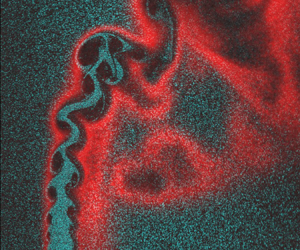
We start with a general qualitative discussion of the SLV evolution, using Mie scattering data. The general structure of the near field is characterized by the roll-up of SLV structures (figure 8) from the jet shear layer, as indicated by the spatially growing vortex regions. These structures eventually saturate in size and strength, and lose coherence further downstream, due to secondary instabilities. Sampling the plane of symmetry in this flow field essentially probes a slice of the jet shear layer, separating the SLV structures into windward and leeward SLV. The significant asymmetry in the leeward/windward development is clearly evident, where the windward shear rolls up and grows much faster than the leeward shear layer. This is due to the much sharper velocity gradients along the windward side, including evidence of reverse flow upstream of the jet (Iyer & Mahesh Reference Iyer and Mahesh2016) while the leeward side has a smaller gradient due to the recirculation region in the wake. As noted earlier, centrifuging in the SLV structures causes regions of low seed density, as clearly evident in these Mie scattering data. While this poses challenges to PIV processing, the size and nature of these observed structures provide qualitative insight into variations between the cases.
Mie scattering data for NR conditions (parameters inset in image).

Starting with the NR, high jet density results ( $S = 1.75$), the images show relatively small vortex cores that grow spatially with downstream distance. Vortex pairing is also evident further along the jet centreline. In contrast, the low density cases (
 $S = 0.35$) show significantly larger vortex structures whose size saturates very near the jet exit, suggesting a much higher growth rate. Similar observations were made by Getsinger et al. (Reference Getsinger, Gevorkyan, Smith and Karagozian2014) who noted that cases with low
 $S$ values showed more rapid vortex roll-up behaviour. With respect to
 $J$, a clear trend is not visible solely from the Mie scattering data; further
 $J$ effect characterization will be provided in the next section.
The streamwise variation in vortical structure coherence also provides some indication of how fast the jet mixes out into the cross-flow. Cases with a faster shear layer roll up and larger vortical structures ( $S = 0.35$ cases) clearly show breakdown of these vortical structures closer to the jet exit. This location at which the jet mixes out into the cross-flow can be identified as the streamwise region where the SLV structures have broken down into smaller scale structures – essentially a measure of the persistence of the jet core. Studies have noted a similar behaviour in free jets (Kyle & Sreenivasan Reference Kyle and Sreenivasan1993), which occurs due to secondary instabilities of these structures (Yule Reference Yule1978) and occur closer to the jet exit for cases with larger spatial growth rate.
The Mie scattering data for the R1 cases show qualitative similarities as the  $S = 1.75$, NR cases. While the roll-up of the windward and leeward shear layers is clearly evident, their size and spatial growth rate is considerably smaller than the high
 $S$, NR case. This is a manifestation of the suppression of the shear layer growth rates, discussed extensively in the literature for both one-dimensional shear layers and for RJICF (Nair et al. Reference Nair, Wilde, Emerson and Lieuwen2019). The low density cases (
 $S = 0.35$) show a more rapid spatial development and roll-up of these vortices, similar to the NR cases. The R1 cases also show evidence of the jet core persisting further downstream relative to analogous NR cases, as indicated by the persistence of large coherent SLV structures further along the jet core. This can be attributed to a slower onset of secondary instabilities and delayed breakdown into small scale turbulence. Similar observations have been made for jet diffusion flames (Yule et al. Reference Yule, Chigier, Ralph, Boulderstone and Ventura1981), where combustion delays the breakdown of vortical structures by slowing the development of secondary instabilities. Further, it is clear that the jet fluid has not mixed out into the cross-flow entirely within the field of view, as evidenced by the fact that the OH-PLIF does not close in on itself, such as is evident in figure 9.
Mie scattering and OH-PLIF data for R1 conditions (parameters inset in image).

Before tackling the R2 flame configurations, consider the variation in radial flame location across the reacting cases ( $\varDelta _{{fl}}$, figure 10). Far enough downstream, this position is controlled by the location at which
 $f_{st}$ is located for a given flow configuration. However, two dependencies can be seen with
 $J$ and the jet fluid temperature
 $T_j$. As the position of
 $f_{st}$ is calculated on an averaged basis, it is dependent on the mixing behaviour of the jet, i.e. cases with stronger mixing will show
 $f_{st}$ further out into the cross-flow, explaining the dependence of
 $\varDelta _{{fl}}$ on
 $J$. The second dependency is tied to the importance of the most reacting mixture fraction, and consequently the local kinetic time scales in controlling the flame position due to elevated jet fluid temperature (R1,
 $S = 1.0$ cases, table 1).
Flame offset  $\varDelta _{{fl}}$ plotted as a function of the mixture stoichiometric mixture fraction,
 $f_{{st}}$, for the R1 (red) and R2 (purple) reacting compositions (table 1); different symbols correspond to different target
 $J$ values for the cases.

On the leeward side, the region of elevated OH region is much broader and correspondingly more loosely correlated with the local flame position. This is primarily because the OH-PLIF signal corresponds to the products of combustion which, in the leeward side, are entrained into the recirculation region in the wake of the jet. In addition, while the windward shear layer mixture fraction profile is sharp, the leeward region is significantly more diffuse and small changes in  $f_{{st}}$ lead to large differences in the spatial position of the flame. These differences can be observed in the spatial location of the leeward OH-PLIF signal between some cases where the signal is contoured with the leeward shear layer (figure 9g), and some where the flame position appears to be completely detached (figure 9c). As such, note two distinct points related to the leeward region – first, there is inherently a higher uncertainty in flame location in this region as determined by OH-PLIF. Second, for related reasons, the flame location is also quite sensitive and will move significantly as a result of small changes in flow velocity and mixing.
Figure 11 provides a similar overlay for the R2 case. These images represent the first documentation of this flame configuration that we are aware of in a JICF. The jet composition for the R2 cases ensures the  $f_{{st}}$ is high enough that the flame tends to sit inside the jet shear layer (
 $\varDelta _{{fl}} < 0$) near the jet core (
 $f = 1$), see figure 10. For the R2 cases, the flame position appears to be insensitive to
 $f_{{st}}$ nominally because both cases have significantly elevated jet temperatures (table 1), and therefore the position is likely governed by the most reactive
 $f$ and local fluid mechanic time scales. The OH-PLIF images also show that the dynamics of the reaction zone for the R2 cases is significantly different from the R1 configuration. Both the windward and the leeward branches of the flame lie completely within the shear layer, as is evident from the lack of elevated OH levels in the leeward zone.
Mie scattering and OH-PLIF data for R2 conditions (parameters inset in image).

Most prominently, there is no indication of any near field SLV structures at all in these images. Farther downstream, the entire jet column clearly undulates over a much larger length scale of approximately  $3\unicode{x2013}4 d_{{j}}$. The absence of regions of high flow rotation rates, i.e. centrifuged pockets, indicates that these structures have significantly lower rotation rates compared with the vortices in the other two configurations. These observations show significantly suppressed SLV growth rates in the R2 case, and dramatically illustrate the importance of radial flame location on the RJICF dynamics.
The suppressed SLV roll-up appears to be controlled by viscous effects. This higher fluid viscosity is not necessarily due to the closer proximity of the flame and the shear layer of the R2 cases, as indicated by  $\varDelta _{{fl}}$ values. For the R1 cases since the flame lies outside the shear layer, the near field shear layer, for the most part, contains relatively cold jet fluid. In contrast, since the shear layer is located outside the flame for the R2 cases, it necessarily contains a mixture of high-temperature products from the fluid passing through the flame surface and the hot cross-flow fluid, leading to a significantly elevated local fluid temperature. The significantly higher local viscosities through the mixing interface can therefore lead to a thicker shear layer as noted by Füri et al. (Reference Füri, Papas, Raïs and Monkewitz2002). Some insight into thickened shear layer effects can be gained from JICF studies using fully developed pipe flows, which similarly have thick shear layers and do show delayed roll-up of the shear layer (Getsinger et al. Reference Getsinger, Gevorkyan, Smith and Karagozian2014). However, regular SLV development and concentration is still clearly observed within 3–4 jet diameters for the non-reacting pipe flow. As such, shear layer thickening alone does not appear to be responsible for suppression of SLV. Rather, Reynolds number effects may be controlling in this situation. Consider a worst case calculation where the entire jet column is at the adiabatic flame temperature, which corresponds to a
 $Re_{{j}}$ of 300–400 (in contrast to the values provided in table 1). These flame images exhibit many qualitative similarities to flow topology of liquid-liquid non-reacting jets in the
 $Re_{{j}} = 200\unicode{x2013}500$ range, which similarly exhibit oscillation of the whole jet flow (Camussi et al. Reference Camussi, Guj and Stella2002), without strong windward SLV roll-up.
3.2. Quantifying SLV behaviour
Having qualitatively discussed key features of the RJICF, we now consider quantitative characteristics. Figure 12 plots the out-of-plane (with respect to the centreplane) vorticity component,  $\omega _z$, while also indicating the individual vortices obtained through the vortex identification technique described earlier. The vorticity in the windward (positive, red) and leeward (negative, blue) shear layers can clearly be seen to roll up into concentrated vortex structures. These specific cases were chosen to highlight the results of applying the vortex identification methodology (§ 2.4) on cases with different growth and rollup behaviour. Distinctions between the SLV characteristics in the different cases, matching the observations from the Mie scattering data, can be observed from the vorticity plots. The degree to which vorticity concentrates into coherent structures can be gauged by comparing the amount of vorticity in the shear layers that is present inside and outside of the indicated vortex cores – recall the vortex core definition decomposes the flow into regions of shear and rotation, and identifies regions of flow rotation that is calculated independently of vorticity. For the NR cases, the majority of the shear layer vorticity lies concentrated inside the indicated vortex cores. Comparing comparable streamwise locations for the R1 cases, while vortex structures are present in the near field, a significant amount of vorticity is present as shear that is distributed along the shear layer, and is not fully concentrated and entrained into the cores. This shows that the concentration of vorticity and roll-up process is slower.
Series of instantaneous vorticity fields (per case) with the vortex structures demarcated as identified using the vortex tracking algorithm (§ 2.4); speckled regions for the reacting cases denote regions of elevated OH-PLIF signal.

For the R2 cases, the shear layer vorticity is very uniformly distributed up to  $x/d_{{j}} \sim 4$ and there is very little concentration of vorticity and vortex cores that are indicative of flow rotation. The lack of large regions of ‘engulfment’ of cross-flow fluid in the near field, driven by rotating vortex cores, further indicates that in the near field the mixing process is dominated by viscous nibbling (Westerweel et al. Reference Westerweel, Fukushima, Pedersen and Hunt2009) as opposed to the irrotational entrainment process described for the NR and R1 cases. In the far field, the spacing between the observed vortices appears to occur over a much longer length scale (3–4
 $d_{{j}}$) compared with the NR and R1 cases, of the order of the jet core undulations noted earlier. In line with the observations of low
 $Re_{{j}}$ JICF (Camussi et al. Reference Camussi, Guj and Stella2002), the near field is dominated by vortical structures with primarily ’negative’ vorticity, analogous to the leeward structures observed here. Although the indicated vortex cores in the leeward regions appear to be influenced by the recirculation in the wake, and do not necessarily correspond to vortex roll-up here. This paints the picture of a significantly more complex flow regime, as suggested by Blanchard et al. (Reference Blanchard, Brunet and Merlen1999) for non-reacting JICF, where there is significant three-dimensional interaction between wake structures including the CVP and roll-up of the shear layer.
Further along the jet trajectory, the next phase of turbulent mixing, diastrophy (Dimotakis Reference Dimotakis1986), can be observed once the vortex structures have saturated in strength and start to breakdown into smaller structures. Differences between the NR and R1 cases can be observed in this phase as well, since the NR cases show a faster transition to smaller structures and the vortex cores in the far field have a highly variable structure with significantly lower peak vorticity. For the R1 cases, coherent vortex cores are still identified as far downstream as  $x/d_{{j}} \sim 6$, matching the observations made in the previous section, suggesting that the transition to smaller scales is suppressed. Given the relatively high
 $Re$ value, this is likely controlled by the appearance of secondary instabilities (Yule et al. Reference Yule, Chigier, Ralph, Boulderstone and Ventura1981), which are clearly suppressed in the R1 case relative to the NR case. Finally, the R2 cases show almost no transition within the field of view since the structures are continuing to concentrate shear layer vorticity as they advect out of the field of view.
To capture this streamwise variation in the vortex strength, the characteristics of the individual vortices identified can be ensemble averaged based on their location with respect to the jet trajectory. The instantaneous jet trajectory is obtained by fitting a standard power-law trajectory to the centre streamline and is shown for an instantaneous velocity field in figure 13(a). The total number of windward vortices through each instantaneous snapshot of a given case is displayed in figure 13(b). Since each vortex has a centroid location in Cartesian space, this can be converted into a streamwise ( $s$) and spanwise (
 $n$) coordinates based on the instantaneous jet trajectory. Streamwise properties of vortex metrics are obtained by averaging over all realizations of the individual vortices present in each ‘bin’ as denoted in figure 13(b). The plots below use a bin width of
 ${\rm \Delta} s = 0.33d_{{j}}$. The uncertainty for the peak swirling strength in each bin can be calculated based on (3.1)
 \begin{equation} \sigma^{2}_{{err}} \cong \sigma^{2}_{{rand}} + \overline{U^{2}_{\langle \lambda_{{ci,0}} \rangle}}, \end{equation}
where  $\sigma ^{2}_{{rand}}$ is the variance within each bin and
 $\overline {U^{2}_{\langle \lambda _{{ci,0}} \rangle }}$ is the root mean square (RMS) of the uncertainty of the peak swirling strength estimate for each individual vortex within the bin. This is obtained by propagating the uncertainty of the velocity fields through the expression for the swirling strength (§ 2.5). The streamwise variation of various vortex metrics provide a quantitative means to track the behaviour of the SLV structures as they roll up, saturate and finally breakdown. Previous studies have used the area (Gharib et al. Reference Gharib, Rambod and Shariff1998), or size of the coherent structures, as well as the circulation to track the strength of the vortices. Here, we also use the peak swirling strength
 $\lambda _{{ci,0}}$ since it quantifies the rotational strength of the vortex structure. The streamwise variation of these three metrics for two NR cases are presented in figure 14 with the uncertainty bounds denoted for the ensembled peak swirling strength,
 $\langle \lambda _{{ci,0}} \rangle$, extracted from the windward shear layer. Note that data from regions below
 $s/d_{{j}} < 1.66$ are not shown because of higher uncertainties due to the resolvable field of view.
(a) Instantaneous vorticity field for  $J = 12, S = 1.75$, NR with identified structures and the instantaneous jet trajectory; (b) ensemble windward shear layer vortex locations based on the centroid displayed with respect to the mean vorticity field; streamwise binning process is highlighted.

Streamwise variation in peak swirling strength  $\langle \lambda _{{ci,0}} \rangle$ for windward and leeward vortices (a,c) and the streamwise variation in circulation and coherent structure size (b,d) for two different NR cases with different
 $S$ and
 $J = 12$; the definitions of
 $\gamma$ and
 $\gamma _{{decay}}$ as indicated in plot (a) are provided in § 3.3.

As the vortical structures roll up from the shear layer, the averaged swirling strength ( $\langle \lambda _{{ci,0}} \rangle$), circulation (
 $\langle \varGamma \rangle$) and vortex area (
 $\langle A \rangle$) increases, as the vortex structures accumulate vorticity through irrotational entrainment (Dimotakis Reference Dimotakis1986). Further on, the
 $\langle \lambda _{{ci,0}} \rangle$ peaks can be attributed to the instability saturating, followed by its decay as the (
 $\omega _z$ oriented) vortical structure weaken, likely due to three-dimensional instabilities and viscous diffusion. In general, any reorientation of the vortex structure away from the centreplane can be interpreted as destabilizing since vorticity contained with respect to the other components (
 $\omega _x$,
 $\omega _y$) are dissipated quickly into the cross-flow due to the strain imparted by the bulk cross-flow. This observation, in contrast to the behaviour of axisymmetric free jets, is supported by previous three dimensional characterization of the SLV structures in turbulent flows (Iyer & Mahesh Reference Iyer and Mahesh2016; Nair et al. Reference Nair2020). The circulation stays elevated further downstream relative to
 $\langle \lambda _{{ci,0}} \rangle$, since its magnitude is governed by the vorticity magnitude contained within the vortical structure which tends to simply expand as it saturates (in contrast to
 $\langle \lambda _{{ci,0}} \rangle$ which can be compared with the peak vorticity). Thus, the circulation can remain elevated even when the instability generating the vortical structures has saturated or even decayed. The area of the vortical structure in general tends to increase monotonically (except for the low density cases) due to the vorticity contained within these structures spreading out due to irrotational entrainment of fluid and diffusion. Thus, the vortical structures detected in the far field tend to be larger and less coherent resulting in a significantly larger variability in detected vortex sizes.
As stated earlier, cases with a lower density ratio show a significantly higher growth rate which can be seen in figure 14(c) since the swirling strength reaches its peak value in the near field close to the jet exit and saturates quickly. In contrast, the growth rate is slower for the higher density ratio case, as manifested in the smaller initial slope and longer distance before saturation. The circulation shows a similar trend between these cases but falls off quickly for the low density ratio cases due to the faster breakdown of coherent structures, as indicated in the Mie scattering data as well. The leeward shear layer in both cases shows a comparatively slower growth rate, in line with initial observations, which is a consequence of the asymmetry in the velocity gradients in the windward and leeward regions. While the above plots were for cases with  $J = 12$, similar results occur across different
 $J$ values which showed consistent trends – strong dependence on
 $S$ and weak dependence on
 $J$.
Results for the reacting cases are presented in figure 15. The R1 cases show a similar trend of initial growth and saturation as the NR cases. Another notable fact is that the peak  $\langle \lambda _{{ci,0}} \rangle$ lies between 1.5 and 1.8 for most NR and R1 cases, collapsing well with respect to the convective flow scales
 $d_{{j}}/u_{{j}}$, an observation shared in earlier work (Nair et al. Reference Nair, Wilde, Emerson and Lieuwen2019). This supports the observations from the Mie scattering data that the fundamental mechanism of shear layer roll-up and growth is similar between the NR and R1 datasets. But, the R1 cases clearly show slower growth rates relative to the NR case, as manifested by the lower values of the initial slopes and the peak location occurring further downstream; i.e. at
 $s/d_{{j}} \sim 3$ and
 $\sim 4$ for the NR (figure 14a) and R1 (figure 15a) cases, respectively. The circulation and vortex size show similar trends but, being a function of the size of the vortex, is naturally larger on average for the R1 cases due to the entrainment of lower density combustion products into the vortices.
Streamwise variation in peak swirling strength  $\langle \lambda _{{ci,0}} \rangle$ for windward and leeward vortices (a,c,e) and the streamwise variation in circulation and coherent structure size (b,d,f ) for R1 and R2 cases with different
 $S$ and similar
 $J$.

Finally, we consider the R2 case (figure 15e), where the Mie scattering data suggested dramatically suppressed shear layer roll-up. In line with this,  $\langle \lambda _{{ci,0}} \rangle$ is significantly flatter with peak values about half that of the NR and R1 cases and the peak location occurring at roughly twice the downstream location. The much slower concentration of shear layer vorticity into coherent structures is also manifested by the fact that these vortex metrics could not be calculated with reasonably uncertainties in the near field regions (
 $s/d_{{j}} < 4.5$) and, hence, are not indicated, which can also be noted from figure 12. Notably, the leeward swirling strength is stronger than the windward in this case. This can be attributed to the fact that the regions of rotation identified in the near field R2 leeward shear layer do not correspond to SLV structures, as noted earlier (figure 12). In addition, while the trend of stronger windward shear layers is noted across most cases (NR and R1) in this study as well as in turbulent jet literature (Getsinger et al. Reference Getsinger, Gevorkyan, Smith and Karagozian2014), this trend can reverse in the low
 $Re_j$ regime (Camussi et al. Reference Camussi, Guj and Stella2002).
3.3. Shear layer growth, saturation and decay
This section further quantifies the shear layer growth rates and peak/saturated values, in order to more readily compare across the different  $J$,
 $S$ and reacting cases, using the streamwise
 $\langle \lambda _{{ci,0}} \rangle$ values. We define the spatial growth rate (
 $\gamma$) with respect to the maximum normalized, ensemble-averaged vortex strength (
 $\langle \lambda _{{ci,0}} \rangle _{{max}}$) and location along the jet centreline (
 $s_{{max}}$) at which this is attained (figure 14a) as
 \begin{equation} \gamma = \left.\left(\frac{\langle \lambda_{{ci,0}} \rangle_{{max}} d_{{j}}}{u_{{j}}}\right) \right/ \left(\frac{s_{{max}}}{d_{{j}}}\right). \end{equation}
The growth rate is plotted for all cases as a function of  $J$ in figure 16. For the NR cases (blue, Figure 16), the growth rate scales strongly most clearly with
 $S$, and exhibits a more weak and non-monotonic dependence upon
 $J$. The
 $S = 0.35$, NR cases show the highest initial growth rate. This is in line with observations from previous studies which have noted that low density (
 $S < 0.45$) jets exhibit globally unstable behaviour (Getsinger et al. Reference Getsinger, Hendrickson and Karagozian2012), which very quickly saturates. Moving to higher
 $S$ values reduces the growth rate, an effect similar to the behaviour of non-reacting free jets (Monkewitz & Sohn Reference Monkewitz and Sohn1988) and planar mixing layers (Brown & Roshko Reference Brown and Roshko1974). Moving on to the reacting configurations, it is clear that the R1 cases (red, figure 16) show a slower growth rate (
 $\gamma$) compared with analogous NR cases. Between the R1 cases, for the most part, the same dependence of growth rate on
 $S$ is observed. Presumably, the reacting cases are governed by some ‘effective’ density ratio that is different from
 $S$, based on the gas expansion ratio and where the flame lies in the R1 configurations (outside the shear layer). For example, comparing results at the same
 $J = 18$ values, note that the growth rate of the R1,
 $S = 0.35$ cases is comparable to the NR,
 $S = 1.75$ case. Finally, considering the R2 cases (purple, figure 16) the initial growth rate is highly suppressed, having values that are 3–5 times lower than the R1 case and about 6–8.5 times lower the NR cases.
Growth rate ( $\gamma$) for each case with the measured value of
 $J$; colours correspond to the flame configuration – NR (blue), R1 (red) and, R2 (purple); lines connect cases with constant target
 $S$ values as indicated in the legend.

From a linear stability perspective, the growth rate of the shear layer is in general, inversely proportional to the momentum thickness  $\theta$ of the jet. But,
 $\theta$ requires the extraction of density measurements in the near field, which is not feasible in the current study. To provide some additional perspective on the observed growth rates, the vorticity thickness
 $\delta _{\omega }$ is calculated as
 \begin{equation} \delta_{\omega} = \frac{u_j}{(\partial v/\partial y)_{max}}, \end{equation}
at the location  $s/d_j = 1.5$.
 $\delta _{\omega }$ has been used as an analogue to
 $\theta$ in other non-reacting (Brown & Roshko Reference Brown and Roshko1974) and reacting (Füri et al. Reference Füri, Papas, Raïs and Monkewitz2002) studies on growth rates in density stratified shear layers. Figure 17 demonstrates that observed growth rate variations do not scale with
 $\delta _{\omega }$. The
 $J = 6$ cases have the largest
 $\delta _{\omega }$ similar to the observations made in non-reacting JICF (Megerian et al. Reference Megerian, Davitian, de B. Alves and Karagozian2007). In addition, the
 $S = 0.35$, NR cases show the largest shear layer thickness despite exhibiting the largest growth rate. Notably, the R1 cases have comparable
 $\delta _{\omega }$ to the NR cases despite having a lower growth rate. While the R2 cases have relatively larger
 $\delta _{\omega }$ compared with corresponding R1 and NR cases, this clearly does not scale with the growth rate observed suggesting that any effect of the thickening shear layer is negligible compared with other effects contributing to the R2 topology. A caveat is that
 $\delta _{\omega }$ only estimates the thickening of the shear layer velocity profile due to combustion and density stratification effects but cannot capture
 $\theta$ where large non-monotonic density variations exist, i.e. near a flame.
Vorticity thickness ( $\delta _{\omega }$) measured at
 $s/{d_j} = 1.5$ for each case with the measured value of
 $S$; colours correspond to the flame configuration – NR (blue), R1 (red) and, R2 (purple); lines connect cases with constant target
 $J$ values as indicated in the legend.

Having considered spatial growth rates, we next consider the maximum value of the saturated structure, using  $\langle \lambda _{{ci,0}} \rangle _{{max}}$, and plotted in figure 18. While there are clearly some differences between the non-reacting and the reacting cases, it appears scaling with respect to the jet velocity
 $u_{{j}}$ captures a large amount of the variability across different
 $S$ and
 $J$ values. For most of the cases the normalized peak swirling strength
 $\langle \lambda _{{ci,0}} \rangle _{{max}} d_{{j}}/u_{{j}}$ lie between 1.5 and 1.8, a significantly smaller range between NR and R1 cases compared with the growth rates plotted in figure 16. In other words, the primary difference between the NR and R1 cases is streamwise location of the peak/SLV growth rate, rather than their final peak strength. The somewhat reduced peak strength of the R1 relative to the NR cases could be due to the higher local viscosity. Turning to the R2 cases, they clearly have significantly lower peak swirling strengths, indicative of the inhibition of the shear layer to roll up into strongly rotating structures. In the far field where these vortical structures are formed (figure 12c), the local time scales are unlikely to sustain high swirling rates before these structures breakdown and dissipate.
Peak saturation swirling strength with the measured value of  $J$; colours correspond to the flame configuration – NR (blue), R1 (red) and, R2 (purple); lines connect cases with constant target
 $S$ values as indicated in the legend.

Of course, parameterizing all of the linear and nonlinear SLV amplification processes into a single quantity,  $\gamma$, averages over spatially evolving effects. For example, a closer observation of the streamwise
 $\langle \lambda _{{ci,0}} \rangle$ variations in figures 14 and 15 show that initially there is strong, almost linear growth, followed by a region of slow growth and saturation. This initial growth is a strong a function of the roll-up strength of the shear layer instability while the saturation behaviour is often dependent on different processes, such as three-dimensional instabilities (Coats Reference Coats1996) and local viscosity (Yule et al. Reference Yule, Chigier, Ralph, Boulderstone and Ventura1981). Thus, each of the parameters of interest, specifically combustion, can have a varying effect on the dominant factors in each phase of the instability growth. To illustrate, consider a NR, low density case (figure 14a) where the initial growth rate is rapid but soon tapers off and grows slowly to its peak. In contrast, for a R1, high density case (figure 15a), the
 $\langle \lambda _{{ci,0}} \rangle$ slope is low initially but steadily grows (within the saturation phase) to the peak value. This complexity is apparent even in the simpler case of a two-dimensional vortex sheet, whose spatial growth rate is highly nonlinear (Pozrikidis & Higdon Reference Pozrikidis and Higdon1985). Given these points, we did evaluate other growth rate definitions, including considering the local slope in the very near field region (
 $s/d_{{j}} < 2.0$), but these did not show any significant qualitative differences from the trends represented in figure 16.
Finally, we consider the decay rate of the SLV which is also related to the rate that the jet mixes into the cross-flow. To quantify, we define  $\gamma _{{decay}}$ as
 \begin{equation} \gamma_{{decay}} = \left.\left(\frac{\langle \lambda_{{ci,0}} \rangle_{{max}}-\langle \lambda_{{ci,0}} \rangle_{{0.67}}d_{{j}}}{u_{{j}}}\right)\right/ \left(\frac{s_{{max}}-s_{{0.67}}}{d_{{j}}}\right), \end{equation}
where  $\langle \lambda _{{ci,0}} \rangle _{{0.67}}$ is 67 % of the peak and
 $s_{{0.67}}$ the location at which the value is reached. This value of 0.67 was used to capture the decay processes more local to the peak (as opposed to a smaller value of, say 0.1), noting that the dissipation process is also highly nonlinear (see figures 14 and 15) implying that far downstream of the peak location, the local swirling strength is less indicative of local vortex properties. Additionally, for some of the low growth rate cases, primarily the R2 configurations (figure 15e), the swirling strength does not dissipate significantly within the domain of the data obtained. A sensitivity study to this threshold was performed, including reducing the thresholds for the R1 and NR cases but no qualitative differences in the trends were observed.
The variation in  $\gamma _{{decay}}$ is plotted as a function of
 $\gamma$ in figure 19. In general, note that there is a correlation between the two; i.e. faster growing SLV structures also decay more rapidly and vice versa. For example, the figure clearly shows that the reacting cases have a lower decay rate compared with the non-reacting cases. In addition, the decay rate varies with
 $S$ since low density cases show faster decay from the peak value. The R2 cases show a significantly lower decay rate compared with the R1 and NR cases. Similar observations were previously made in the context of the Mie scattering images (figure 8) where it is clear that low density ratio NR cases, which have significantly faster shear layer growth rates, and consequently larger vortex structures closer to the jet exit, resulting in a faster breakdown of the jet core. Similar observations were also made by Kyle & Sreenivasan (Reference Kyle and Sreenivasan1993) for the case of low density round jets where cases exhibiting self-excited oscillations exhibited breakdown of the jet core closer to the jet exit. This process has been thought to be influenced by the onset of secondary instabilities along these vortical structures and cases which exhibited stronger growth of the primary SLV consequently exhibited faster growth of the secondary instabilities (Yule Reference Yule1978). Similarly, the reacting cases, which in general exhibit suppressed
 $\gamma$ values, clearly show weaker decay rates. A similar rationale was presented by Yule et al. (Reference Yule, Chigier, Ralph, Boulderstone and Ventura1981) with respect to the delayed transition for jet flames (compared with similar non-reacting free jets), noting that the process of ‘re-laminarization’ suppressed the onset of secondary instabilities that contributed to the breakdown of the jet core. To summarize, these results suggest that at leading order the contribution of combustion is primarily through its impact on secondary instabilities and not through changes in viscosity, at least for the R1 cases.
Decay rate ( $\gamma _{{decay}}$) compared with the growth rate (
 $\gamma$); colours correspond to the flame configuration – NR (blue), R1 (red) and, R2 (purple); lines connect cases with constant target
 $S$ values as indicated in the legend; hollow cases denote
 $J = 6$ points.

Note that there are a few outliers to this trend; these outliers are the lowest  $J$ (
 $J = 6$), NR cases (figure 19). One possibility for that case being outliers is that they are globally unstable, as manifested by the rapid vortex roll-up (figure 8a–c) and regularly spaced train of vortices with clear tonal content in the velocity spectra (Getsinger et al. Reference Getsinger, Gevorkyan, Smith and Karagozian2014). However, the
 $S = 0.35$ cases also show strong growth and vortex structures indicative of global instability (Getsinger et al. Reference Getsinger, Hendrickson and Karagozian2012), and those cases (other than the
 $J = 6$ case) do exhibit a good correlation between
 $\gamma$ and
 $\gamma _{{decay}}$. As such, the scatter in these NR,
 $J = 6$ points does not appear to be due to a different scaling between globally and convectively unstable cases. Rather, we hypothesize that this scatter is due to jet trajectory effects. At lower momentum flux ratios, curvature effects due to the bending of the jet into the cross-flow can have a lower influence on the breakdown of these vortical structures compared with cases that penetrate further (Sau & Mahesh Reference Sau and Mahesh2008). As the trajectory approaches a free jet (at higher
 $J$), these effects become less sensitive to
 $J$ since the trajectory is relatively vertical in the near field, around the region where SLV structures for most NR cases appear to saturate. Further, for the R1 cases, since the breakdown process is suppressed, the saturation location is usually further along the jet core across all
 $J$ values (i.e. trajectory shapes), once it has already been reoriented with the cross-flow and therefore does not show the same additional sensitivity to the cross-flow trajectory. In other words, we hypothesize that this scatter arises in cases where SLV growth and decay both coincide with regions of high jet curvature.
4. Discussion and concluding remarks
As emphasized in the introduction, RJICF have many additional degrees of freedom due to combustion. The results presented here capture dominant SLV dependencies upon  $J$,
 $S$ and flame–shear layer offset.
The SLV growth rate was used to quantify the rate at which vorticity concentrates itself into coherent structures. For NR cases, the initial growth rate decreases with increasing  $S$, similar to previous observations (Getsinger et al. Reference Getsinger, Hendrickson and Karagozian2012), but had a weaker dependence on
 $J$ than they reported. This variation highlights the limitations in comparing JICF results across different experiments with different cross-flow boundary layer thicknesses and jet shear layer thicknesses. For example, due to the elevated cross-flow temperatures used here and consequent lower Reynolds number, the current study has a significantly larger cross-flow boundary layer thickness compared with related non-reacting studies that capture variation of jet behaviour with
 $J$ (Megerian et al. Reference Megerian, Davitian, de B. Alves and Karagozian2007). For example, Shoji et al. (Reference Shoji, Harris, Besnard, Schein and Karagozian2020) and Iyer & Mahesh (Reference Iyer and Mahesh2016) show that the counter-current mixing layer parameter, does a better job of correlating data across a range of conditions than
 $J$ alone.
Considering the effect of combustion, the R1 cases clearly show a suppressed growth rate compared with analogous NR cases. Qualitatively, this suppression can be seen in the longer distance taken by the shear layer to completely roll up into concentrated regions of vorticity. This observation is consistent with prior work on nominally two-dimensional shear layers and jet flows, and is dominated by inviscid effects (as opposed to viscous effects associated with the much higher viscosities in the reacting cases) as evidenced by the comparable peak vortex strength values and similar decay rate scalings between the NR and R1 cases. The observation that the R1 cases show the same dependence on the jet density (through  $S$) as the NR cases suggest that, in the near field, the flame changes the ‘relevant’ density ratio across the mixing interface (due to the R1 flame position). Given that the flame induced fluid density is lower than the nominal cross-flow density values, this would correspond to density ratios larger than
 $S$ for analogous jet fluid density values – in line with the assertion that increasing
 $S$ decreases the growth rate.
As mentioned above, the fact that peak saturation values between the NR and R1 cases are similar, as well as the correlation between growth and decay rates, suggests that the growth, peak and decay of the SLV can be explained largely from inviscid arguments. For example, the negative correlation between the decay and growth rate supports the hypothesis that the breakdown process is strongly linked to the onset of secondary instabilities, while viscosity likely plays a secondary role. Finally, since the breakdown process is largely correlated with  $\gamma$, this parameter can easily be correlated with the mixing performance of the jet, across both R1 and NR configurations.
The R2 cases demonstrated completely different shear layer behaviour compared with the NR and other reacting (R1) condition, demonstrating that the above arguments do not generalize to this case. The flow is almost completely devoid of concentrated vortical structures, as the annular vortex ring emanating from the jet remains distributed along the streamwise direction. Consequently the growth rates are significantly lower compared with R1 and NR conditions. Viscosity effects appear to be very important in this case, both in creating a locally thicker shear layer (i.e. less susceptible to roll up) and a very low  $Re_{{j}}$. In other words, while combustion causes the same reduction in local
 $Re_{{j}}$ in both the R1 and R2 cases, its effect is much more profound in R2 cases as it occurs in the jet rather than the cross-flow. There are similarities in the centreplane flow topology of the R2 cases and non-reacting low
 $Re_{{j}}$ configurations, manifested as long wavelength jet core undulations similar to an elliptical instability of the CVP, proposed by Blanchard et al. (Reference Blanchard, Brunet and Merlen1999).
This work also suggests several promising lines of future study. These results quantify the behaviour of the SLV structures with respect to the commonly used JICF parameters,  $J$ and
 $S$ as well as the effect of combustion and flame position. But, the limitation of these parameters in uniquely predicting the shear layer behaviour is apparent since these parameters do not quantify the local conditions at the near field shear layer that strongly influence the SLV dynamics. The counter-current shear layer model evaluated by Iyer & Mahesh (Reference Iyer and Mahesh2016) and Shoji et al. (Reference Shoji, Harris, Besnard, Schein and Karagozian2020) shows promising path towards extracting metrics that can better parameterize JICF dynamics, suggesting future work to extend this model to describe the RJICF stability behaviour. Another area of future work is more detailed characterization of the three-dimensional development of the SLV and appearance of the CVP. For example, this work showed a dramatically different flow dynamics for the R2 case from the ‘classical’ JICF structure, suggesting comparable differences in other flow structures. Given that the CVP structure is highly correlated with the SLV vortex roll-up process (Getsinger et al. Reference Getsinger, Gevorkyan, Smith and Karagozian2014), it is possible that the CVP either does not develop at all or is significantly weakened, implying poor mixing in the far field. A more exhaustive study focusing on the velocity data in transverse planes (
 $x$–
 $z$ and
 $y$–
 $z$), and across a larger parameter space would address this question.
Declaration of interest
The authors report no conflict of interest.
Funding
This work was partially supported by the National Science Foundation under contract number 1705649 (contract monitor Dr. H. Chelliah).


 Open access

