

1 Introduction
The literature generally presents the period 1870-1913 as the high watermark of 19th century globalization (Daudin et al. Reference Daudin, Morys and O'Rourke2008), which is known as the First Globalization to contrast it with the post-World War II (WWII) process of international integration. However, there is also agreement that, during the period 1870-1913, the advance of international integration itself triggered a retreat from pro-global postures (Williamson Reference Williamson1998, Reference Williamson2002). This retreat has been explained as a protectionist backlash: partly in response to the grain invasion of continental Europe caused by technological improvements in transport (O'Rourke Reference O'Rourke1997) and partly as a reply of the European periphery to the customs increases of its core-country partners (Blattman et al. Reference Blattman, Clemens and Williamson2003; Williamson Reference Williamson2006). In any case, the popular wisdom is that there was an anti-globalization reaction during the globalization process during 1870-1913 that, for Spain, has been traditionally associated with the protectionist changes of the 90s.
First, in December 1890, as a declared response to the drop in transport costs, duties on grain and meat were substantially increased in Spain. A year later, in December 1891, as part of a strategy to force France to negotiate a new treaty, duties on manufactured goods were also increased. The resulting rise in customs, because of its intensity, has led the literature to talk about a 90s protectionist swerve (the viraje proteccionista, Serrano-Sanz Reference Serrano-Sanz1987). Moreover, part of the academic community has claimed that the deterrent effect of raised customs on imports was then reinforced by the simultaneous depreciation of the Spanish peseta (Prados de la Escosura Reference Prados de la Escosura1988, Reference Prados de la Escosura1997; Prados de la Escosura and Tena Reference Prados de la Escosura and Tena1994).
Therefore, three main barriers have supposedly influenced Spanish trade during 1870-1913 (international transport costs, customs and currency) and the aim of this paper is to disentangle the role that each one played over time by using a gravitational approach. The approach, of course, is not new. In the last decade, a number of works have analyzed the forces that drove trade during the First Globalization by introducing different measures of, or proxies for, trade barriers into a gravity equation (Estevadeordal et al. Reference Estevadeordal, Frantz and Taylor2003; López-Córdova and Meissner Reference López-Córdova and Meissner2003; Flandreau and Maurel Reference Flandreau and Maurel2005; Mitchener and Weidenmier Reference Mitchener and Weidenmier2008; Jacks and Pendakur Reference Jacks and Pendakur2010).
However, none of these papers have compared the specific evolution of the different trade barriers for the period 1870-1913, which is the comparison we carry out for Spain. In this task, we can exploit a range of measures of customs barriers, instead of using proxies or the traditional ratio of customs revenues over total imports used in multi-country analyses to date. Moreover, given that for most of the period under examination, the peseta exchange rate was in a floating regime, instead of the traditional dummies used in multi-country panels to capture the effects of adherence or non-adherence to the gold standard, we consider the size and sign of the peseta exchange rate departures from parity between 1870 and 1913 and their effects on trade.
The results from estimating the gravity equation for different panel data samples confirm that, whatever the customs variable considered, transport costs and currency variables are always significantly linked to imports. However, the customs variable only appears significant when considering the measures that control for the sample of goods over time. This might explain the difficulties experienced by some studies in finding a significant relationship between customs and imports when using the simple ratio between customs revenues and total importsFootnote 1.
More interestingly, as we have directly estimated the elasticity of substitution for Spanish imports, we can combine the three kinds of variables into a costs function to obtain a single measure of barriers to trade. According to our estimations, this synthetic measure, the trade costs tariff equivalent, averaged an ad valorem tariff of 112 per cent during 1870-1913, 65 points coming from transport costs, 22 from customs and only 7 from the exchange rate. Thus, on average, the exchange rate seems to have played a minor deterrent role compared with that of the other barriers. This finding fits in with the idea of those who hold that, in the long run, the peseta played a minor role as a trade barrier.
However, when instead of static averages, we consider the evolution of the trade costs tariff equivalent and its three components over time, the resulting picture tells a much richer story. To start with, we find that the peseta acted both as a barrier to and a boost for trade at different moments during the period. In the 80s, the exchange rate moved under parity contributing, together with customs and transport, to a reduction of the trade costs tariff equivalent. This is in clear contrast to what happened in the 90s, when a chain of exceptional depreciations that culminated in the year of the defeat against the United States (1898) raised a currency barrier which, added to the increased customs, broke the downward trend of the tariff equivalent. Once the war was over, the peseta adjusted to a new movement of appreciation that significantly reduced its height as a barrier. Therefore, we find that the exchange rate played an active role during the period 1870-1913, in some periods reinforcing the movement of customs, in others playing an offsetting role. In this way, this paper reconciles the two positions, one assigning a minor long-run role and the other an active short-run role to the peseta as a barrier, that coexist in the literature.
Finally, the aforementioned reversal in the downward trend of the trade costs tariff equivalent confirms the 90s as the moment of the Spanish protectionist backlash. The breaking down of the tariff equivalent into its components illustrates how, before the 90s, the sharp reduction of transport costs ran in parallel to a slight decrease in customs, both contributing, along with the exchange rate, to the decline of the Spanish trade costs tariff equivalent. In the 90s, however, the increase in customs stopped the falling trend of the tariff equivalent, thus reflecting the Spanish backlash against the drop in transport costs and the abandonment of the premises of free trade in continental Europe, especially in France.
The result is the story of anti-globalization within globalization to which we have referred. As a sign of globalization, the Spanish tariff equivalent average decreased between 1870-1890 and 1891-1913, although to a much lesser extent than if currency and, especially, customs had not raised barriers in the 90s. Without the anti-globalizing role played by the Spanish idiosyncratic barriers to trade (customs plus currency), we have estimated that the decline in transport costs would have trebled the growth of imports at the end of the period 1870-1913.
The rest of the paper is organized as follows: in the second section, we present the procedure and data used in the estimation of the gravity equation. In the third section, we discuss the evolution of the trade costs tariff equivalent and relate the dynamics shown by its three components to the historical narrative. In the fourth section, we conclude.
2 The procedure and data
As we have said, our goal is to establish the channels whereby different sources of costs affected Spanish trade in the First Era of Globalization. To this end, we consider three kinds of directly measured barriers (customs, maritime transport costs and exchange rates) that are introduced into a gravity equation à la Anderson and van Wincoop (Reference Anderson and van Wincoop2003). These authors, starting from a constant elasticity of substitution (CES) utility function where the prices of imported goods reflect «iceberg» trade costs, propose the following gravity equation:

where Xij denotes exports from country i to country j; Yi and Yj represent the respective national GDPs; Y w is the total world income and σ the elasticity of substitution between products; tij is the bilateral trade cost factor (one plus the tariff equivalent of trade barriers) and Πi and Pj denote country i's and country j's price indexes. The specific expression of these price indexes is:
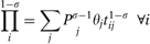

where θi denotes the share of world income of country i.
Anderson and van Wincoop (Reference Anderson and van Wincoop2003, Reference Anderson and van Wincoop2004) refer to Πi and Pj as multilateral resistance indexes since, by construction, they consider the average trade resistance between a country and its partners. Index Πi weighs the trade costs of country i when exporting to all its partners. Index Pj weighs the trade costs imposed by importer country j to all its partners. To explain bilateral trade flows, the bilateral trade cost factor has to be compared to the product of the multilateral indexes. The authors summarize the rationale for this comparison as follows: Given a bilateral barrier between i and j (tij), a higher multilateral resistance of country j (higher barriers in j for other partners; Pj) will reduce the relative prices of goods from i and increase its exports to j. Analogously, a higher multilateral resistance of country i (higher barriers faced by i from other partners; Πi) will reduce the supply price of goods from i and increase its exports to j.
Given our specific interest in analyzing Spanish imports, we express equation [1] as:

where Msi denotes Spain's imports from country i, Y s is the Spanish GDP and Ps represents Spain's multilateral resistance.
Thus, the theoretical stochastic expression in which we are interested becomes:

We assume that the bilateral trade cost factor tis can be defined as a multiplicative function of different trade barriers, tis = Π (Zis n)λn, where Zis n (n = 1…N) denote the barriers and λn are the observable individual elasticities of each component Zisn. Finally, if we introduce the trade costs function tsj into equation [3], we obtain the expression:

or more specifically, since we consider three kinds of barriers (customs, ct; currency, CU; and maritime transport costs, tcr), the expression to estimate is (where all the variables are in logs):

Starting from this equation, the estimation of coefficients for the three barriers γn = (1−σ)λn n = 1,2,3, enables us to compute the individual elasticities in the trade costs function as λn = γn/(1−σ) and the tariff equivalent for each barrier Zn as (Zis n)λn. This is possible since, according to Feenstra (Reference Feenstra2002, Reference Feenstra2004), when working with the simple customs average, the coefficient estimated in a gravity equation is equal to (1−σ). This means that the elasticity λ 1 = 1 or, in other words, the tariff equivalent for the simple customs average is the average itself. Therefore, we can derive the elasticity value from the γ 1 coefficient, then calculate the elasticities for the other two barriers and, finally, combine the customs, currency and transport costs tariff equivalents into a multiplicative trade costs function to obtain a synthetic trade costs tariff equivalent.
The data used to calculate this synthetic tariff equivalent come from the following sources. The availability of data for the period 1870-1913 allows us to work with a sample of twenty countries (Australia, the Austro-Hungarian empire, Belgium, Brazil, Canada, Denmark, Finland, France, Germany, the Netherlands, Italy, Japan, Norway, New Zealand, Portugal, Sweden, Switzerland, Uruguay, the United Kingdom and the United States). National GDPs (expressed in 1990 Geary-Khamis dollars) come from Maddison (2009). As regards the bilateral flows, import figures have been obtained from the Spanish annual Foreign Trade Statistics, first converted to dollars and then to 1990 dollars with the U.S. deflator of Taylor (Reference Taylor2002). The value of Spanish imports from these countries averaged 80 per cent of total imports during 1870-1913. The figures for total exports in domestic currency come from Mitchell (Reference Mitchell2003a, Reference Mitchell2003b, Reference Mitchell2003c) and have been converted to dollars by applying the exchange rates in the Global Financial Data site (http://www.globalfindata.com) and then corrected by the U.S. deflator.
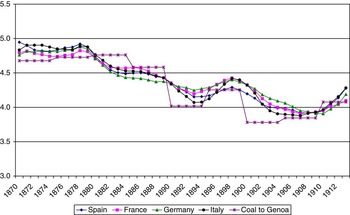
As previously mentioned, three different kinds of barriers are included in our trade costs function: maritime costs, customs tariffs and those associated with exchange rates. Starting with maritime shipping costs, there is a pervasive agreement that these costs registered an overall declining trend during the period 1870-1913, as shown by Mohammed and Williamson (Reference Mohammed and Williamson2004) in their real global freight rate index. The same occurs with the indexes of country-pair specific freight rates offered in Jacks and Pendakur (Reference Jacks and Pendakur2010). These authors construct indexes between the United Kingdom and 21 other countries for the period 1870-1913, and conclude that freight rates fell on average by 50 per cent in this period. In Figure 1, we show the paths of shipping costs between the United Kingdom and Spain and between the United Kingdom and Spain's main trade partners, all of which are quite reminiscent of the pattern shown by the commodity- and city-specific Coal to Genoa freight rate index of Mohammed and Williamson (Reference Mohammed and Williamson2004). The indexes of transport costs of Jacks and Pendakur (2010) are used in our estimation while, as explained later in the paper, the indexes of Mohammed and Williamson (Reference Mohammed and Williamson2004) are used to test the robustness of the results.
SHIPPING FREIGHT RATES BETWEEN THE UNITED KINGDOM AND SPAIN AND SPAIN′S MAIN PARTNERS
Source: Jacks and Pendakur (Reference Jacks and Pendakur2010) and Mohammed and Williamson (Reference Mohammed and Williamson2004).

More specifically, we use the United Kingdom–Spain freight rate series of Jacks and Pendakur (2010) to proxy the evolution of bilateral Spanish shipping costs with its main partners and also with Austria, Belgium, the Netherlands and Portugal. The indexes between the United Kingdom and Australasia, Brazil, Canada, Denmark, Japan, Sweden–Norway (for Sweden, Norway and Finland), the United States and Uruguay are taken as representative of the respective maritime transport costs between Spain and each of these countries that, once again, follow a clear downward trend. By doing so, we are assuming that, for the nearest countries, the United Kingdom–Spain index is representative of the evolution of Spain's short-haul freight rates. For the most distant countries, we are assuming that the deeper downward trends registered by the United Kingdom routes are representative of the evolution of Spain's long-haul freight ratesFootnote 2. Of course, we are conscious that the transport revolution of the 19th century was not limited to shipping. There was also a decline in land transport costs associated with the spread of railroads. However, we assume that, for a peninsular country like Spain, maritime transport played the most important role in explaining its integration into the world marketFootnote 3.
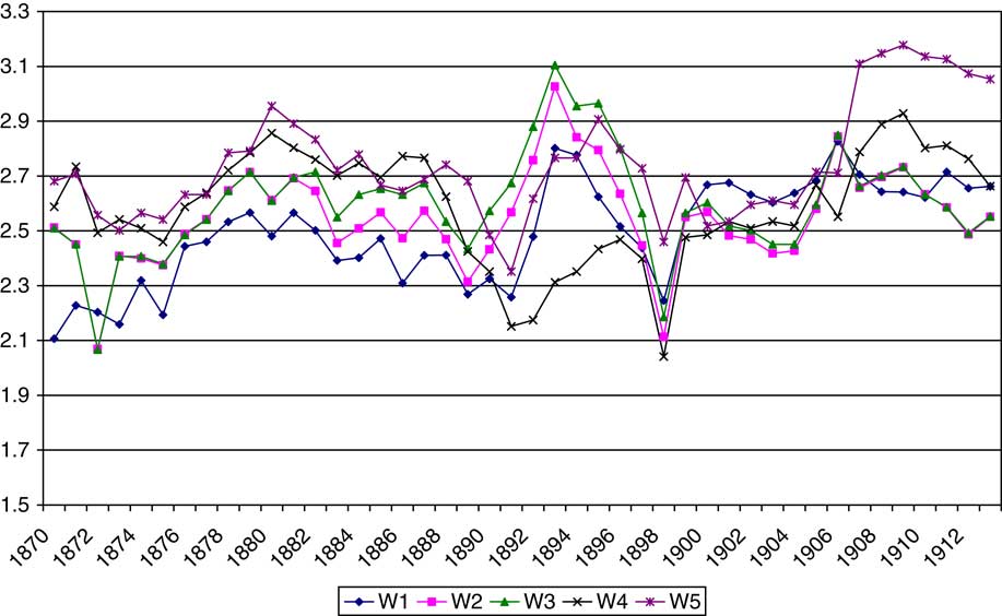
Concerning tariff barriers, in Figure 2, we show different measures of trade-weighted nominal protection. The trajectory of Weighted 1 corresponds to the ratio of tariff revenues over the value of total imports as registered in the official Spanish Foreign Trade Statistics. It is worth remarking that, in the Spanish case, the unreliability of official import unit values introduces significant bias into the calculation of the ad valorem rates of protectionFootnote 4. For this reason, we also work with measures such as Weighted 2 and Weighted 3 that take into account the falsity of the import unit values in the official statistics. Weighted 2 is calculated by dividing the tariff revenue by the corrected import values in Prados (Reference Prados de la Escosura1986). Weighted 3 comes from Tena (Reference Tena2006), who adds the surcharges on sugar imports to the import revenues. We have modified these three series to take into account the payment of Spanish tariffs in gold from 1906 on, which meant an appreciable surcharge on dutiesFootnote 5. Payment in gold is also taken into account in the trade-weighted measure Weighted 4 constructed by Tirado (Reference Tirado1994). In this case, the official values are also corrected but, instead of considering all products registered in the Spanish Foreign Trade Statistics during 1870-1913, the author uses an unchangeable selection of highly representative goods over the period. In Weighted 5, the sample only considers the industrial goods in Weighted 4. Therefore, both these indexes have the advantage of avoiding the risk that variations in the aggregate measure might simply be reflecting variations in the goods composition of trade, thus blurring the relationship between commercial policy and trade.
TRADE-WEIGHTED CUSTOMS TARIFFS
Source: Prados (1986), Tirado (Reference Tirado1994) and Tena (Reference Tena2006).
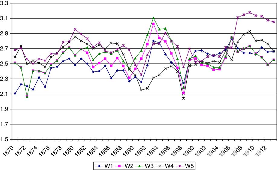
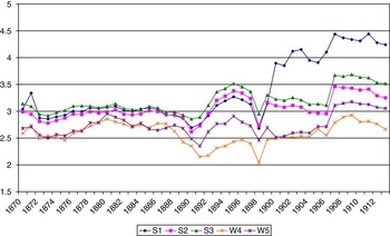
However, as is well known, trade-weighted averages endogenize the constraint effect of customs increases on trade and, consequently, there is always a bias of undervaluation in these measures. The higher the tariff applied to a certain good, the lower its imports and, consequently, the lower the weight of the highest taxed goods in the calculation of the aggregate level of protection. For this reason, it is important to have, as well as trade-weighted averages, simple arithmetic averages which, in turn, are the type of measures to consider in a theoretically well-founded version of the gravity equation. The simple arithmetic average, Simple 1, shown in Figure 3 along with Weighted 4, is offered in Tirado (Reference Tirado1994), both of them for the same sample of representative goods mentioned above. Simple 2 is the simple arithmetic average once overseas products have been excluded. It is clear how both simple averages, as expected, reach higher values than the weighted rate. The same occurs if we compare Weighted 5 to Simple 3, where the latter is the simple average for the industrial goods included in Simple 1. This point is also illustrated for Spain by Tena (Reference Tena1999), when comparing different customs measures for a number of years during the period 1870-1913. The levels are always higher for simple than weighted measures, whether the latter are weighted by actual trade or the trade structure prior to the enforcement of a new bill. In any case, the interruption of the declining trend of tariff barriers in the 90s is a common feature for all the yearly series mentioned above, including the profile shown by the estimations of Tena (Reference Tena1999). Therefore, as previously mentioned, we can exploit a range of measures of customs barriers, although none of them are available in bilateral terms, a shortcoming which we consider minimized because the Most Favoured Nation Clause was the rule for Spain's commercial policy during 1870-1913.

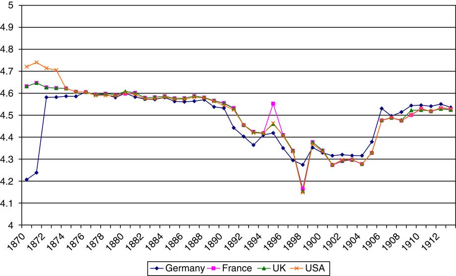
Finally, we have considered the role played by the peseta exchange rate in Spanish external trade. Unlike most western currencies, the peseta never formally belonged to the gold standard, there being only a partial gold convertibility from 1876 to 1882. In Figure 4, we show the performance of the nominal rates of the peseta against its main partners’ currencies which, after Germany adhered to gold in 1871 and the United States won the battle against silver in 1874, exhibit a noticeable parallelism in their evolutionFootnote 6. The Spanish lack of commitment to gold emerges clearly in the early 90s. It was then that the peseta began to depreciate and this depreciation gathered pace in the years of the war against Cuba and the United States (1895-1898). After this plunge in its external value, the Spanish currency adjusted to a path of recovery until the end of the period.
NOMINAL EXCHANGE RATE INDEXES FOR GOLD CORE COUNTRIES
Source: Global Financial Data.
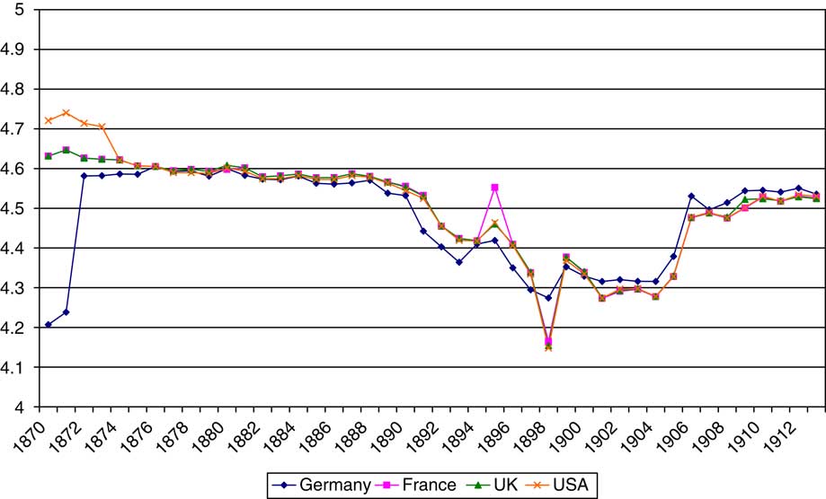
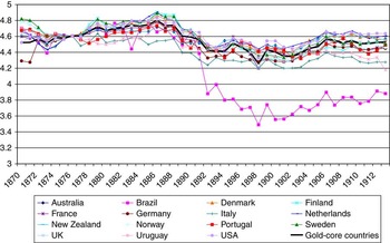
Our interest in the exchange rate, however, goes beyond its nominal evolution. Its role, either as a barrier to or as a boost for imports, depends on whether the interaction between nominal rates and relative prices determines episodes of real depreciation or appreciation for the peseta, respectively. Therefore, we focus on the peseta real exchange rates, which we calculate for the countries with available data by correcting the nominal rate through the corresponding relative price index (Spanish over foreign prices). The prices are GDP deflators: the Spanish deflator comes from Prados (Reference Prados de la Escosura2003) and the foreign ones from Mitchell (Reference Mitchell2003a), except for the Dutch, Portuguese and Uruguayan figures that come from Smits et al. (Reference Smits, Horlings and van Zaden2000), Lains (Reference Lains2006) and Bértola (mimeo), respectively. The indexes of real exchange rates are shown in Figure 5. Here again, we find a very similar evolution of the peseta exchange rates against most of the currencies considered, consistent with their general commitment to gold. In fact, the two countries with the shortest commitment, Italy and Brazil, especially the latter, are those that exhibit the weakest adjustment to the gold core-countries’ real exchange averageFootnote 7.
REAL EXCHANGE RATE INDEXES
Source: Mitchell (Reference Mitchell2003a), Prados (Reference Prados de la Escosura2003), Bértola (mimeo), Smits et al. (Reference Smits, Horlings and van Zaden2000) and Lains (Reference Lains2006).

For the gold currencies, the evolution of the peseta real exchange rate goes through three stages. First, there is a movement of real appreciation in the 80s, which turns into a movement of depreciation in the 90s. Once the war is over, the peseta adjusts to a new trend of real appreciation. We select the profile depicted by the core-countries’ average as representative of the evolution of the peseta real exchange rate for all the countries in our sample (including those for which we have no information) except for Italy and Brazil, for which we will consider their respective real exchange rate indexesFootnote 8. In the next section, we examine how these real exchange rate indexes along with maritime transport costs and customs influenced the performance of Spanish imports in the First Era of Globalization.
3 Anti-globalization within globalization
As observed in the previous section, the expression to estimate is:

However, some practical problems arise. In theory, the difference between the prices of countries i and s included in the gravity equation should reflect the effect of relative trade barriers on bilateral flows, for which the available price indexes can only be considered as a proxy. Consumer price indexes and GDP deflators include non-tradable goods prices and, furthermore, certain trade barriers are not reflected in prices. For this reason, Feenstra (Reference Feenstra2002) and Anderson and van Wincoop (Reference Anderson and van Wincoop2003) proxied the multilateral_resistance effect by using source and destination region fixed effects. However, with our data panel, which covers only one country (Spain) during a relatively short period (1870-1913), the use of country-year effects would leave us without enough degrees of freedomFootnote 9. Neither can we solve the problem by using country-period effects (country dummies interacting with 2-, 3-, 4- or 5-year-period dummies) because of problems of multicollinearityFootnote 10. Therefore, we propose an alternative way to proxy the multilateral resistance effect on the basis of the model of Anderson and van Wincoop (Reference Anderson and van Wincoop2003), summarized in Section 2.
According to these authors, the bilateral trade cost factor between i and j (in our case, the barrier between country i and Spain, tis) has to be compared to the product of the multilateral indexes (country i's and Spain's price indexes, Πi and Ps). The rationale for this comparison is that, given a bilateral barrier between i and Spain, a reduction in barriers faced by i from other partners will raise its total exports, increasing the supply price of i’s goods and reducing its exports to Spain. Thus, if we read an increase in i’s total exports as the result of a reduction in its multilateral barriers, one way to proxy the multilateral resistance depressing effect of this on i's exports to Spain is to discount the value of i's total exports from Yi. By doing so, we are reducing i's exporter potential to Spain. Analogously, given a bilateral barrier between i and Spain, a reduction in the barriers between Spain and the rest of its trade partners will increase the relative prices of goods from i and reduce Spanish imports from country i. Thus, if we read an increase in its total imports from third partners as the result of a decrease in its multilateral barriers, one way to proxy this other multilateral resistance depressing effect on Spanish imports from i is to discount the value of Spanish total imports (except i's) from Y s. By doing so, we are reducing the Spanish importer potential from country i.
Consequently, our instrumental version of the gravity equation is as follows:

where Yi* and Ys* denote i's and Spain's GDPs, after discounting the levels of country i's total exports and Spain's imports from third countries, respectively.
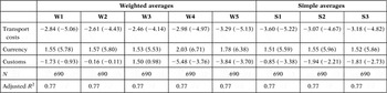
We use several measures of customs protection and the indexes of maritime freight rates of Jacks and Pendakur (Reference Jacks and Pendakur2010)Footnote 11. We have also considered the real exchange rate of the peseta over time as a potential influence on Spanish imports. The results of combining these different measures, after imposing the standard assumption of unit elasticity on the adjusted economic size variables, are shown in Table 1. The first finding to highlight is that transport costs are always highly significant. The same occurs if, when testing for robustness, we proxy the trends of shipping costs by the city- and commodity-specific indexes of Mohammed and Williamson (Reference Mohammed and Williamson2004)Footnote 12. The exchange rate is also always significant. However, the only significant tariff measures (Simple 1, Simple 2, Simple 3, Weighted 4 and Weighted 5) are those that keep the sample of goods unchanged over the period under study. The difference between the coefficients of the simple and weighted measures is also important. The coefficients for the weighted measures are significantly higher than those corresponding to the simple measures (Weighted 4 vs. Simple 1, both calculated for the whole unchanged sample; Weighted 5 vs. Simple 3, both calculated for the industrial unchanged sample), in line with the criticism of undervaluation against the former mentioned above. From here on, we will focus on the results obtained when considering simple customs averages and, particularly, the Simple 2 average, calculated for the unchanged sample of goods with the exclusion of overseas foodFootnote 13.
GRAVITY ESTIMATIONS OF TRADE COSTS

W, weighted; S, simple.
Notes: W1 calculated with official values; W2, W3, calculated with corrected values, the latter including sugar surcharges; W4 calculated with corrected values maintaining the sample fixed; W5, as W4, for only industrial goods.
S1 calculated for the same sample as W4; S2 is S1 without overseas products; S3, for the same sample as W5.
Estimations are country-fixed effects.
Source: See text.
This average is a simple one and therefore, as explained before, we assume that its individual elasticity λ 1 = 1 and calculate the elasticity of substitution starting from the estimated coefficient γ 1 = (1−σ). Since the coefficient obtained for the protection measure is 1.94, we find that the elasticity of substitution among Spanish imports is 2.94 when transport costs and fluctuations in the real exchange rate are controlled for. This is an interesting result because it is directly estimated from the panel data and is near the usual elasticity values found in the literatureFootnote 14.
By using our estimated elasticity of substitution among the Spanish imports, we calculate that the elasticities of the maritime freight rates and the peseta real exchange rate in the trade costs function are 1.58 and −0.80, respectively. This yields a trade costs tariff equivalent, τ, that averages 112 per cent during 1870-1913, 65 points coming from transport costs, 22 from customs and 7 from the exchange rateFootnote 15. Our estimated trade costs tariff equivalent is above those computed by Jacks et al. (Reference Jacks, Meissner and Novy2010). These authors, by assuming a price elasticity of imports of 11 (σ = 11), derive a comprehensive measure of trade costs for the United Kingdom, France and the United States, which ranges from a minimum of around 30 per cent (in the United Kingdom in 1913) to a maximum of 48 per cent (in the United States in 1870). However, our tariff equivalent level is not directly comparable to theirs. First, our assumption about the level of maritime transport costs to which to apply the indexes of Jacks and Pendakur (Reference Jacks and Pendakur2010) is overestimating our tariff equivalent levelFootnote 16. Second, they hypothesize a high elasticity value, which might be underestimating their tariff equivalents.
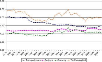
Fortunately, the comparison of levels is not the goal of this paper. Rather than in the absolute level of the trade costs tariff equivalent and its average during 1870-1913, which are clearly sensitive to the elasticity considered, we are interested in the changes in the dynamics of its components (transport costs, commercial policy and currency). We are looking for a confirmation of the Spanish protectionist backlash against the decline in international transport costs and the supposedly protectionist role played by a currency that did not join the gold standard. To this end, the trajectories of the trade costs tariff equivalent and its components, not seriously affected by the elasticity value chosen, are far more informative. Looking at Figure 6, we find that the tariff equivalent was reduced from 156 per cent to 104 per cent between 1870 and 1913 and, above all, we find that the trends shown by its components match the economic history narrative perfectlyFootnote 17. Behind the downward trend in the transport costs component, it is easy to recognize the technological improvements in maritime shipping (among them, the introduction of the screw propeller, the compound engine, steel hulls and the increase in ship sizes)Footnote 18. We also find that the slight decrease in the customs and exchange rate components during the 80s matches the historical record.
TRADE COSTS TARIFF EQUIVALENT AND COMPONENTS

On May 11, 1882, Spain signed a treaty with France in which the two countries exchanged significant concessions. Spain agreed to cut customs for many manufactured items and France, in exchange, substantially reduced duties on the Spanish import of wine, from 3.5 to 2 francs/hectolitre. More importantly, soon after this, the Spanish reductions agreed in the treaty were included as a second column of duties in the bill of July 1882. This second column was applied to the countries that enjoyed the Most Favoured Nation Clause in their relationship with Spain, which, in the mid-80s (after the Modus Vivendi signed with the United Kingdom in 1885), applied to more than 90 per cent of the value of Spanish importsFootnote 19.
In the same direction as customs, the exchange rate also facilitated the entry of foreign goods into Spain. In 1870, at the beginning of the period under examination, the Spanish monetary standard was bimetallic (gold and silver) and, for that reason, was fully affected by the sustained decline in the international price of silver initiated in 1867. This fall in prices meant silver overvaluation at the mint. Minting silver became a profitable business and silver coins quickly started to oust increasingly valuable gold from circulation. To put an end to this process, the Spanish authorities declared their intention of abandoning bimetallism in favor of gold and prohibited the private mintage of silver through a decree in August 1876Footnote 20. Nevertheless, despite this measure, budgetary problems led the Spanish government to continue the profitable minting of silver while continuing to monetize deficits through bond sales to the Bank of SpainFootnote 21. In this way, the growth in fiat money (overvalued silver and paper), by offsetting the continuous hoarding of gold, was enough to increase the Spanish money supply and isolate domestic prices from the international deflation of the 70s.
During this decade, however, the pressure on the reserves of the Bank of Spain was kept under control. As mentioned before, the peseta never formally belonged to the gold standard. Convertibility was always a discretional issue for the Bank which, in fact, repeatedly limited this possibilityFootnote 22. The problems, however, did not become unsustainable until the 80s when the drop in capital inflows caused by the French stock crisis depreciated the peseta enough to make the export of gold profitable, thus stimulating paper conversion. As a consequence, despite the Bank having rationed convertibility, its gold reserves were reduced from 126 million pesetas in 1881 to 61 million in 1882. When, in 1883, the reserves decreased to 36 million pesetas, the Bank decided to suspend convertibility and it would never be resumed. However, despite price divergence, the peseta nominal exchange rate remained quite stable after the suspension, thanks to the exceptional exports of wine to France along with the offsetting role played by private exports of goldFootnote 23. The result was a real appreciation of the peseta in the 80s, which, combined with the simultaneous decrease in maritime freights and customs barriers, explains the fall in the total tariff equivalent in that decadeFootnote 24.
However, in the early 90s, as shown in Figure 6, this harmony of declining barriers was broken and, while transport costs continued to go down, the Spanish customs component started to rise. In fact, the first step in the Spanish tariff protectionist reform of 1890-1891 was defended as a means to offset the declining prices of grain imports resulting from technological advances in transport. As a result of this competition, the price of wheat in Barcelona had decreased from 26.7 to 22.3 pesetas/hectolitre between 1880 and 1885, pushing down the domestic average from 23.9 to 19.9 pesetas, respectivelyFootnote 25. As a first response to this internationally induced drop in domestic prices, several measures aimed at improving productivity were takenFootnote 26. However, as time went by and gains in efficiency failed to stop the advance of imports, the decision was taken to reinforce protectionFootnote 27. In December 1890, tariffs on grains and rice were raised. Tariffs were also increased on meat, whose imports, coming from Australia and Argentina, had registered a great increase in the 80s due to the combined effect of declining transport costs plus refrigerationFootnote 28. In this way, Spain started the retreat from liberalization that characterized the reaction of continental Europe to the land rent losses brought about by the grain invasion from Russia and overseasFootnote 29. The retreat mirrors the social significance of landowners in the Spain of the late 19th centuryFootnote 30.
The second step in the retreat was the approval of the bill of December 31, 1891, which, as well as including the raised tariffs on agrarian products, increased most of the customs for manufactured items. The reason argued for this remarkable increase in the duties on manufacture was one of strategic policy. In January 1891, France had denounced the treaty signed with Spain in 1882, meaning that, from February 1892, if a new treaty were not agreed upon, Spanish wine would have to pay the duties resulting from the tariff reform then in progress in the French Assembly. As is well known, the Méline bill, finally passed in December 1891, included a generalized increase in customs that was especially punishing for Spanish wine because its duties were raised from the previous range of between 2 and 3.5 francs/hectolitre to another of between 14.8 and 19.8 francs. The Spanish response consisted of inflating the duties on manufactures in its bill of 1891, also approved in DecemberFootnote 31, and then offering France a treaty that included a cut in duties on Spanish manufactures in exchange for a reduction in French duties on Spanish wineFootnote 32. To reinforce the appeal of the proposal, Spain offered these cuts in exclusivity. However, France's interest in the Spanish market was much less than Spain's in the French. In 1890, Spain received only 5 per cent of total French exports, while France received 45 per cent of total Spanish exports. This meant that Spain had to negotiate by attacking «with a needle against one defending with a sword»Footnote 33 and, not surprisingly, the treaty was never signed. Having lost the main market for its principal export (wine), Spain only exchanged minor concessions with other countries (through treaties with the Netherlands, Norway, Sweden and Switzerland), which were far less important marketsFootnote 34. In the end, the result of the whole process (the 1891 bill and the four treaties mentioned) was a significant increase in customs at the beginning of the 90s. Accordingly, Figure 6 shows a rise of the customs component that is in clear contrast to the decline registered by the transport costs component.
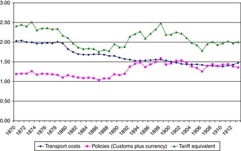
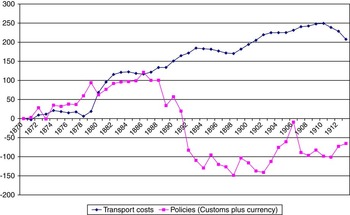
As regards the movements of the exchange rate in the 90s, they contributed to the trade costs tariff equivalent in the same direction as commercial policy, that is to say, by increasing it. This common pattern can be clearly seen in Figure 6 and even more so in Figure 7, where the Spanish policy barriers (customs and exchange rate) have been added. The agrarian crisis of the mid-80s seriously affected tax revenues, a significant deficit reappeared and the sale of bonds to the Bank resumed to such an extent that, in 1890, fiat money accounted for more than 80 per cent of legal tender. In these circumstances, the Baring crisis in Argentina, by spreading doubts about the solvency of countries with a weak treasury, led to a sharp drop in the capital flows to Spain. The result was a significant depreciation of the peseta, which did not recoup part of its losses until 1895, just before plummeting again as a consequence of the risk that the markets assigned to the Spanish debt because of the strongly renewed monetization of deficit to finance the war against Cuba and the United States. In sum, the risk assigned to the Spanish Treasury led to a decade of real depreciation for the peseta, which worked as a barrier for imports. More importantly, the effect of this depreciation, added to the increase in customs barriers, was enough for the Spanish trade costs tariff equivalent to regain a substantial part of the level to which it had fallen in the 80sFootnote 35.
TRADE COSTS TARIFF EQUIVALENT, TRANSPORT COSTS AND POLICIES

The financial disorders of the war years, however, were quickly addressed. A number of measures taken in 1899-1900 allowed the budget to close with a surplus, debt held by the Bank of Spain was redeemed and prices were stabilizedFootnote 36. The restoration of confidence in the Spanish Treasury plus the renewal of foreign investment inflows (now focused on electricity and water services) are the reasons put forward to explain the recovery, in 1906, of the nominal exchange rate levels prior to the Baring crisis. From then on, the relative control of public finances and domestic prices determined the stability of the exchange rate at around 26 pesetas to the pound and, as shown in Figure 6, the exchange rate significantly reduced its role as a trade barrier.
At this point, it is worth highlighting the changing trends of the exchange rate component, since these changes allow us to reconcile some apparently divergent stances taken in the literature regarding the consequences of Spain not having belonged to the gold standard. Returning to Figure 6, it is clear that the performance of the exchange rate component is consistent with the ideas of Prados de la Escosura (Reference Prados de la Escosura1988, Reference Prados de la Escosura1997), Prados de la Escosura and Tena (Reference Prados de la Escosura and Tena1994), Tortella (Reference Tortella1994) and Sánchez-Alonso (Reference Sánchez-Alonso1995), among others, when arguing that the movements of the peseta reinforced the protection approved in the tariff bill of 1891 and reduced that approved in the bill of 1906. However, the trajectory of the exchange rate component also supports the ideas of Serrano-Sanz et al. (Reference Serrano-Sanz, Gadea and Sabaté1998) and Gadea and Sabaté (Reference Gadea and Sabaté2004), who, finding evidence in favor of the purchasing power parity (PPP) hypothesis, argue in favor of a moderate role of the peseta in terms of protection. In their opinion, the holding of the hypothesis means discarding the idea that remaining out of the gold standard led to a continuous increase or decrease of competitiveness for Spain. In this regard, the figure of 7 per cent that the exchange rate component averages in the period 1870-1913 is consistent with a long-run moderation in protectionist terms. In the same way, the variations in the trend of the exchange component shown in Figure 6 match the significant short-run deviations from parity found by Serrano-Sanz et al. (Reference Serrano-Sanz, Gadea and Sabaté1998) and Gadea and Sabaté (Reference Gadea and Sabaté2004) for the 80s (deviations of appreciation) and for most of the 90s (deviations of depreciation)Footnote 37. These variations serve to reconcile positions: in the short run, the exchange rate played an active role (reinforcing or loosening commercial barriers); in the long run, the average effect was smoothed.
As regards transport costs and customs components, while the former continued to follow a downward trend in the first decade of the 20th century, the latter moved upward. Thus, the counterbalancing role of transport costs and customs tariffs continued and this became especially clear when the bill of 1906, by raising duties, restored the ad valorem customs levels of the 90sFootnote 38. In sum, two dynamics clearly emerge, one before and one after 1890, when comparing the evolution of transport costs and customs components in Figure 6. Before the 90s, the sharp reduction in transport costs took place in parallel with a slight decrease in customs and, thus, the decline in the Spanish trade costs tariff equivalent was essentially driven by the path of maritime freight rates. However, in the 90s, the increase in customs barriers started an offsetting relationship between them that the tariff reform of 1906 sustained. Thus, from 1890 onward, especially when the exchange rate barrier was lowered, trade policy becomes the most active force in defining the profile of the Spanish trade costs tariff equivalent.
Finally, in Figure 8, we present this counterbalancing relationship in terms of the accumulated contributions of the different barriers to the variations in the ratio between Spanish trade and economic growth. According to this figure, the decline in transport costs, had the customs and the exchange rate barriers remained unchanged, would have trebled the growth of imports in 1913. Also in the figure, it is easy to observe the offsetting role of customs plus currency barriers after 1890. During the subperiod 1870-1890, customs and currency as well as transport costs had contributed positively to the growth of imports. In contrast, during the subperiod 1891-1913, the gains in the contribution of transport costs were severely offset by the negative contribution of Spanish policy barriers, especially in the decade of the 90s, when customs and exchange rate barriers rose in similar fashion.
CONTRIBUTIONS TO THE GROWTH OF SPANISH IMPORTS.
Source: see text.

4 Conclusions
This paper estimates the relationship between three potential kinds of trade barriers (transport costs, customs and currency) and Spanish imports during 1870-1913. First, we find that customs tariffs have a significant negative impact on trade as long as the selected protection measure controls for the goods composition. We also show how the use of trade-weighted measures, normally employed in these estimations, downwardly biases the estimated effect of customs on imports. Second, whatever the customs measure, transport costs and exchange rate always show a significant effect on imports, both with the expected sign. Third, on the basis of their significance, we have combined the three kinds of variables into a trade costs function to obtain a single measure of trade barriers. This yields a trade costs tariff equivalent average of 112 per cent ad valorem during 1870-1913, with only 7 points coming from the exchange rate. As remarked before, the moderate height averaged by the currency barrier during 1870-1913 fits in with the idea of the peseta having played a long-run minor deterrent role on trade. Even so, in the short run, as revealed by the evolution of the exchange rate component, currency made significant (positive and negative) contributions to the trade costs tariff equivalent. Thus, this paper reconciles the short- and long-run approaches to the analysis of the protectionist consequences of the fact that the peseta never formally belonged to the gold standard. Finally, our estimations locate the start of an offsetting relationship between decreasing transport costs and increasing customs barriers in the 90s, in tune with the historical record, which dates the Spanish protectionist backlash to the tariff reform of 1890-1891.