1 Introduction
Perturbed flow over a mildly uneven terrain is a classic topic that is encountered in countless applications. It is often mathematically formulated as a linearized problem, in which the slope of the boundary is assumed to be small, and this is the setting we shall also adopt in this paper. It goes without saying that for larger slope many other phenomena complicate the matter, most prominent being flow separation and detachment, but this will be assumed not to occur here, or possibly to be accounted for by the adoption of an approximate artificial boundary.
Linearization of the problem with respect to the slope of the boundary implies, of course, that any desired result is a linear functional of such slope, and therefore can be expressed through a transfer function in wavenumber space. In simplified words, once we have solved the problem for a sinusoidal boundary we have solved it for any (shallow enough) curvy boundary (there included an isolated bump). Transfer functions allow a tremendously powerful generalization, and are probably one of the main reasons why linearization is so useful. In what follows we shall particularly focus our attention on the transfer function from boundary slope to shear stress exerted on the boundary.
Seminal in this subject is the paper by Benjamin (Reference Benjamin1959), and much of the present discussion will be based upon this author’s problem set-up, and on the modified Orr–Sommerfeld equation introduced by Thorsness et al. (Reference Thorsness, Morrisroe and Hanratty1978). Just like Benjamin, we shall initially restrict the discussion to laminar flow and then examine its possible implications for turbulent flow. This theory appears to have been discovered more than once, and its generalization to turbulent flow by Hunt and coworkers (Jackson & Hunt Reference Jackson and Hunt1975; Belcher & Hunt Reference Belcher and Hunt1993) still to this day provides the foundation of a large number of geophysical applications (Belcher & Hunt Reference Belcher and Hunt1998).
In addition to linearization, the definition of a transfer function requires a translation-invariant problem; namely, the base flow has to be approximated as locally parallel and all of the classical approaches do so. Even though the locally parallel approximation of a spatially evolving boundary layer is itself a classical topic (and a large part of Benjamin’s derivation is devoted to setting it up properly), here we show the surprising result that in some wavenumber range non-parallel effects of boundary-layer growth can drastically affect the shear-stress transfer function, and the locally parallel result turns out to be incorrect. On the other hand, as will also be seen, an inner–outer matched asymptotic expansion coupling boundary layer and potential flow provides the correct answer, because it does not parallelize the boundary layer at leading order and respects its symmetries.
The material is organized as follows. In § 2 we define the notation and the governing equations along the lines of Benjamin (Reference Benjamin1959), and introduce the basic goal of our analysis: the transfer function from boundary slope to wall shear stress in wavenumber space. In § 3 we go through the asymptotic analytical solutions of this problem, outlining a consistent framework of the various regimes that are encountered with varying wavenumber
 $k$
and of the approximations appropriate to each. In § 4 we move to examining numerical solutions, which are not difficult for this one-dimensional problem but produce a surprising outcome: the numerical and asymptotic results are inconsistent with each other! Section 5 proposes the solution of this conundrum: It appears that essential to the asymptotic solution were symmetry properties of the boundary layer, which were instead lost in the parallel Orr–Sommerfeld approximation of Benjamin. Hanratty’s formulation, originally introduced to better account for curvature of the streamlines in turbulence models, turns out to possess the power to restore the correct invariance properties in laminar flow, as will be illustrated here in more than one way. The compared numerical solutions of Benjamin’s and Hanratty’s formulation are taken up in § 6, where a number of examples will be shown in different regimes. The numerical solution of Hanratty’s formulation will also be used to confirm the accuracy of a simple analytical formula, previously derived in § 3, which describes the range of
 $k$
where the transfer function is largest. Up to this point only laminar flow is considered; extensions of the theory to turbulent flow are the subject of § 7. After going through the, sometimes radical, changes that occur in the definition of the asymptotic regimes because of the different scaling of laminar and turbulent flow, numerical solutions will be examined first in the quasi-laminar regime where the perturbation still only feels laminar viscosity even though the mean flow has a turbulent profile, and then in the presence of a turbulence model the limitations of which will be shown.
2 Problem set-up
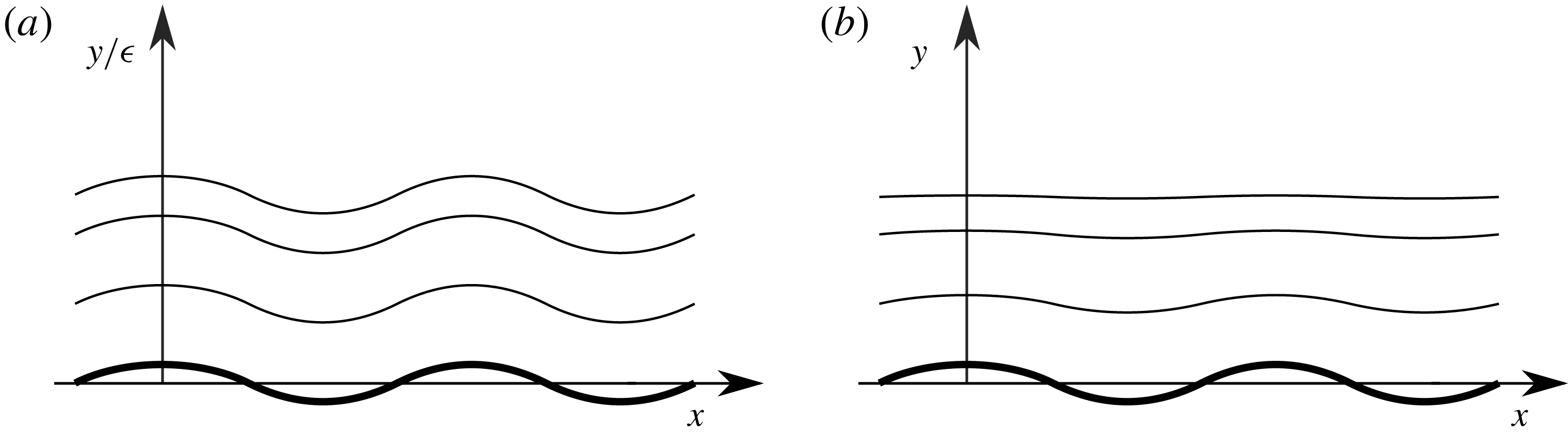
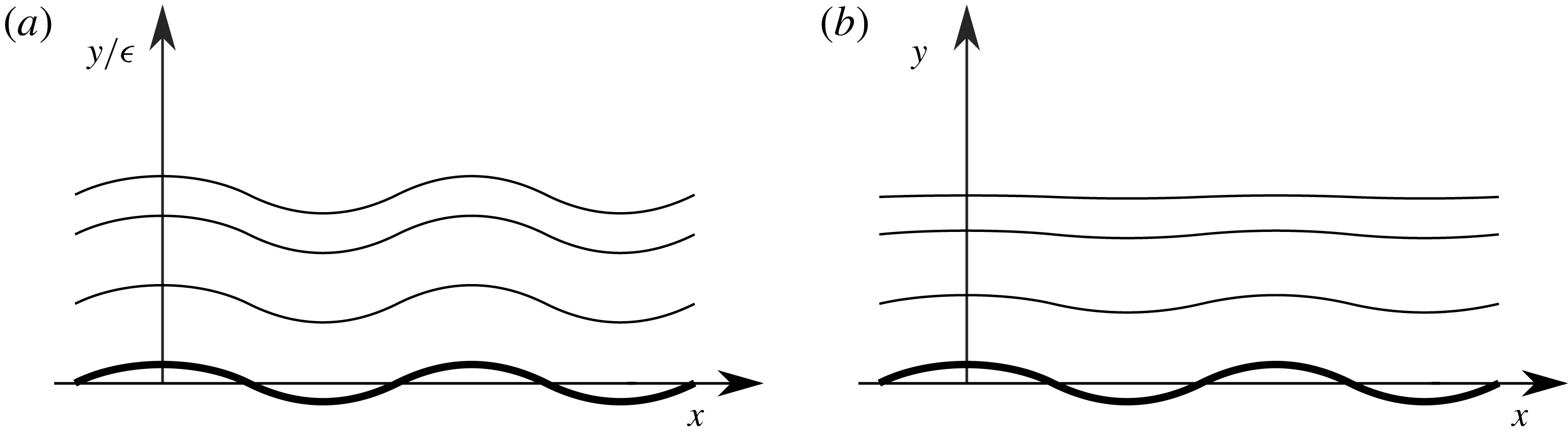
Flow past a wavy boundary can occur in a confined or in an open geometry. A two-dimensional channel closed by two walls (or by a wall and a free surface) can be virtually infinite in length, and the canonical unperturbed laminar flow in it is without question Poiseuille flow. On the other hand, an open flow cannot be completely translation invariant (with the notable exception of unbounded Couette flow, which constitutes an important limiting case), and must be envisaged as a locally parallel portion of an otherwise non-parallel boundary layer. Benjamin (Reference Benjamin1959), having the excitation of water waves by wind as the primary application in his mind, devoted a large part of his first sections to the approximations involved in setting up the open, quasi-parallel problem properly. If the region nearest to the wall is assumed to be governed by Prandtl’s boundary-layer equations for both the base flow and its perturbation, a well-known fundamental symmetry of these equations allows an arbitrary vertical displacement as an exact solution. This solution has a very simple geometrical interpretation: if Prandtl’s equations were an exact mathematical representation, every streamline of the perturbed flow would geometrically mould so as to keep the same distance from the wall it had before the perturbation (see figure 1). With increasing distance from the wall Prandtl’s equations must eventually fail, in a closed channel because the streamline would not fit the opposing wall and in an open space because potential flow tends to damp streamline curvature but, Benjamin argued, the linearization is more easily justified, and acceptable over a more extended range, if performed in curvilinear coordinates that follow the wall’s geometry.
After a thorough examination of the order of magnitude of each and every non-parallel term, for which we refer the reader to the original paper, he concluded that the problem can safely be approximated by the locally parallel Orr–Sommerfeld equation ((3.2) on p. 173 of Benjamin Reference Benjamin1959), the stationary form of which we shall rewrite as
 $$\begin{eqnarray}-\text{i}k(U\unicode[STIX]{x1D713}^{\prime \prime }-U^{\prime \prime }\unicode[STIX]{x1D713}-k^{2}U\unicode[STIX]{x1D713})=k^{4}\unicode[STIX]{x1D713}-2k^{2}\unicode[STIX]{x1D713}^{\prime \prime }+\unicode[STIX]{x1D713}^{\prime \prime \prime \prime },\end{eqnarray}$$
with boundary conditions ((2.7) and (2.9) on p. 169 of Benjamin Reference Benjamin1959)
 $$\begin{eqnarray}\unicode[STIX]{x1D713}(0)=0;\quad \unicode[STIX]{x1D713}^{\prime }(0)=-hU^{\prime }(0).\end{eqnarray}$$
These are, in fact, the same equation and boundary conditions that could have been obtained in Cartesian coordinates by linearizing the Navier–Stokes equations about a parallel flow directly. Therefore, Benjamin’s procedure can be seen as a theoretical justification for doing the latter.
A formulation alternate to Benjamin’s was given by Hanratty and coworkers in a series of papers (Zilker et al.
Reference Zilker, Cook and Hanratty1977; Thorsness et al.
Reference Thorsness, Morrisroe and Hanratty1978; Abrams & Hanratty Reference Abrams and Hanratty1985). As explained in particular by Thorsness et al. (Reference Thorsness, Morrisroe and Hanratty1978), who ascribe the development to Thorsness (Reference Thorsness1975), they introduced a ‘boundary-layer coordinate system’ in which they moved the origin of the
 $z$
coordinate to the displaced surface
 $z=h(x)$
before the linearization, like Benjamin did, but crucially the base flow was moved together with the coordinate system, and thus assumed to have the velocity
 $U(z-h)$
, i.e. the same velocity profile that would exist on a plane surface but displaced to the new origin. As will be discussed in greater detail in § 5, this slight modification has deep implications.
Streamlines follow the wall in a boundary layer of thickness
 $\unicode[STIX]{x1D716}$
(a), but not in potential flow (b).
As far as notation is concerned, the only difference between the present equation (2.1) and (3.2) of Benjamin (Reference Benjamin1959) for
 $c=0$
(steady wall waviness), is non-dimensionalization. Here we use viscous units (the same that in a turbulent flow are called wall units), in which the non-dimensional viscosity, unperturbed shear stress and unperturbed wall velocity gradient are all unitary. Namely, using a subscript ‘dim’ for dimensional quantities (with the exception of
 $u_{\unicode[STIX]{x1D70F}}$
, which is dimensional by definition), we adopt the following notation:
 $$\begin{eqnarray}\left.\begin{array}{@{}c@{}}u_{\unicode[STIX]{x1D70F}}=\sqrt{\unicode[STIX]{x1D70F}_{dim}/\unicode[STIX]{x1D70C}_{dim}};\quad z=z_{dim}u_{\unicode[STIX]{x1D70F}}/\unicode[STIX]{x1D708}_{dim};\\ k=k_{dim}\unicode[STIX]{x1D708}_{dim}/u_{\unicode[STIX]{x1D70F}};\quad \unicode[STIX]{x1D6FF}=\text{Re}_{\unicode[STIX]{x1D70F}}=\unicode[STIX]{x1D6FF}_{dim}u_{\unicode[STIX]{x1D70F}}/\unicode[STIX]{x1D708}_{dim}.\end{array}\right\}\end{eqnarray}$$
Primes denote derivatives with respect to the wall-normal coordinate
 $z$
,
 $k$
is the longitudinal wavenumber and
 $\unicode[STIX]{x1D713}(z)$
is the perturbation streamfunction, whereas
 $U(z)$
is the unperturbed velocity profile, defined as
 $U_{dim}(z_{dim})=u_{\unicode[STIX]{x1D70F}}U(z_{dim}u_{\unicode[STIX]{x1D70F}}/\unicode[STIX]{x1D708}_{dim})$
. The velocity profile extends up to a typical boundary-layer thickness (or channel half-height)
 $\unicode[STIX]{x1D6FF}_{dim}$
, whose dimensionless value
 $\unicode[STIX]{x1D6FF}$
in viscous units identically coincides with the usual definition of the shear-based Reynolds number
 $\text{Re}_{\unicode[STIX]{x1D70F}}$
. This identity will be emphasized where appropriate, but it should be remembered that in the presence of two length scales,
 $\unicode[STIX]{x1D6FF}_{dim}$
and
 $\unicode[STIX]{x1D706}_{dim}=2\unicode[STIX]{x03C0}/k_{dim}$
, both
 $\unicode[STIX]{x1D6FF}$
and
 $k^{-1}$
can in turn play the role of a Reynolds number. The dimensionless function
 $U(z)$
is by definition such that
 $U(0)=0$
,
 $U^{\prime }(0)=1$
,
 $U_{ext}=U(\infty )=O(\text{Re}_{\unicode[STIX]{x1D70F}})$
for laminar flow and
 $U_{ext}=U(\infty )=O(\log \text{Re}_{\unicode[STIX]{x1D70F}})$
for turbulent flow.
The Fourier transform
 $\widehat{h}(k)$
of the boundary perturbation
 $z=h(x)$
(where
 $z=0$
is the reference flat wall) is defined according to the convention:
 $$\begin{eqnarray}\displaystyle \widehat{h}(k)=\int _{-\infty }^{\infty }h(x)\text{e}^{\text{i}kx}\,\text{d}x,\quad h(x)=\frac{1}{2\unicode[STIX]{x03C0}}\int _{-\infty }^{\infty }\widehat{h}(k)\text{e}^{-\text{i}kx}\,\text{d}k, & & \displaystyle\end{eqnarray}$$
and the transfer function from boundary slope to wall shear-stress perturbation
 $\unicode[STIX]{x1D70F}_{1}$
is
 $$\begin{eqnarray}T(k)=\frac{\widehat{\unicode[STIX]{x1D70F}_{1,dim}}/\unicode[STIX]{x1D70F}_{dim}}{\widehat{\text{d}h_{dim}/\text{d}x_{dim}}}=\frac{\widehat{\unicode[STIX]{x1D70F}_{1}}}{-\text{i}k\widehat{h}}=\frac{\widehat{\unicode[STIX]{x1D713}}^{\prime \prime }(0)+\widehat{h}U^{\prime \prime }(0)}{-\text{i}k\widehat{h}}.\end{eqnarray}$$
Fourier transforms and perturbation quantities will be implicitly understood wherever not ambiguous, with hats and 1 subscripts omitted.
3 Asymptotic description
The solution of (2.1) was tackled by Benjamin through asymptotic techniques similar to those that had been adopted before him for stability problems, and to those which would give origin in the coming years to triple-deck theories. Without pretension of being exhaustive, this section will give an overview of the relevant formulas. We start with some order-of-magnitude considerations, valid for laminar flow only. Revised estimates for turbulent flow will be the subject of a separate section, § 7. For
 $k\gg 1$
(small
 $\unicode[STIX]{x1D706}$
-based Reynolds number), the problem (2.1) reduces at leading order to creeping Stokes flow. This limit was examined in Charru & Hinch (Reference Charru and Hinch2000) with the result that
 $$\begin{eqnarray}T(k)\simeq 2\text{i}\,\text{sign}(k)+0.5k^{-2}.\end{eqnarray}$$
For
 $k$
smaller than
 $1$
, a viscous and an inviscid wall-normal scale of length come into play, in addition to the unperturbed boundary-layer thickness
 $\unicode[STIX]{x1D6FF}$
. The inviscid length scale is dictated by the Laplace equation: it is simply
 $k^{-1}$
. The typical viscous scale emerges from a study of Couette flow (Charru & Hinch Reference Charru and Hinch2000, see also § 3.1 below), and turns out to be
 $k^{-1/3}$
. Since
 $k\ll 1$
, the viscous scale is always much smaller than the inviscid scale. The Orr–Sommerfeld equation (2.1) now lends itself to further local approximations.
For
 $z\ll k^{-1}$
, equation (2.1) can be replaced by the linearized boundary-layer equation
 $$\begin{eqnarray}\displaystyle & -\text{i}k(U\unicode[STIX]{x1D713}^{\prime }-U^{\prime }\unicode[STIX]{x1D713}+p)=\unicode[STIX]{x1D713}^{\prime \prime \prime }, & \displaystyle\end{eqnarray}$$
 $$\begin{eqnarray}\displaystyle & p^{\prime }=0, & \displaystyle\end{eqnarray}$$
 $p$
, which was hidden in (2.1), has been made explicit for later use. As is easily verified, taking the derivative of (3.2a
) makes the pressure disappear and reproduces (2.1) up to terms
 $O(k^{2})$
.
For
 $z\gg k^{-1/3}$
, equation (2.1) instead loses its right-hand side and reduces to the inviscid Rayleigh equation, which with pressure made explicit can be written as
 $$\begin{eqnarray}\displaystyle & U\unicode[STIX]{x1D713}^{\prime }-U^{\prime }\unicode[STIX]{x1D713}+p=0, & \displaystyle\end{eqnarray}$$
 $$\begin{eqnarray}\displaystyle & p^{\prime }=-k^{2}U\unicode[STIX]{x1D713}. & \displaystyle\end{eqnarray}$$
 $k^{-1/3}\ll z\ll k^{-1}$
,
 $k^{2}$
can be neglected and (3.3b
) becomes
 $p^{\prime }=0$
. Or, equivalently,
 $\unicode[STIX]{x1D713}^{\prime \prime \prime }$
can be neglected and (3.2a
) becomes (3.3a
). (3.3a
) then has the analytical solution
 $$\begin{eqnarray}\displaystyle & p=\text{const.}, & \displaystyle\end{eqnarray}$$
 $$\begin{eqnarray}\displaystyle & \displaystyle \unicode[STIX]{x1D713}(z)=U(z)\left[B_{1}-p\int _{z_{1}}^{z}U^{-2}\,\text{d}z\right], & \displaystyle\end{eqnarray}$$
 $z_{1}$
is arbitrary and constant
 $B_{1}$
changes with it.
In a region of constant unperturbed velocity (
 $z\gg \unicode[STIX]{x1D6FF}$
,
 $U=U_{ext}$
), which may or may not overlap with one of the previous regions, equations (3.3) reduce to the potential-flow equations
 $$\begin{eqnarray}\displaystyle \unicode[STIX]{x1D713}^{\prime \prime }-k^{2}\unicode[STIX]{x1D713} & = & \displaystyle 0,\end{eqnarray}$$
 $$\begin{eqnarray}\displaystyle U_{ext}\unicode[STIX]{x1D713}^{\prime }+p & = & \displaystyle 0,\end{eqnarray}$$
 $$\begin{eqnarray}\unicode[STIX]{x1D713}(z)=\unicode[STIX]{x1D713}(0)\exp (-|k|z).\end{eqnarray}$$
The boundary condition classically associated with potential flow,
 $$\begin{eqnarray}\unicode[STIX]{x1D713}(0)=-hU_{ext},\end{eqnarray}$$
is notably different from the viscous boundary condition (2.2), but as is generally known and will be reasserted below, it consistently follows from a boundary-layer analysis.
Finally, in the region
 $k^{-1}\lesssim z\lesssim \unicode[STIX]{x1D6FF}$
, if such a region is non-empty, i.e. if
 $k\unicode[STIX]{x1D6FF}\gg 1$
, (3.3) admit no simplification and must be retained in full. Different flow regimes will occur (even for the same base flow with varying
 $k$
) according as the boundary-layer thickness
 $\unicode[STIX]{x1D6FF}$
traverses each of the above regions.
3.1 The Couette-flow region
Starting from
 $k\gtrsim 1$
(regime 0, creeping flow, described by (3.1)) and progressively reducing
 $k$
(increasing
 $\unicode[STIX]{x1D706}=2\unicode[STIX]{x03C0}/k$
), we shall first encounter a regime where both the viscous and the inviscid scale are smaller than the thickness of the unperturbed boundary layer. The velocity profile
 $U(z)$
can then for all purposes be replaced by the first term of its Taylor expansion,
 $U(z)=z$
, and the boundary-layer equation (3.2a
) becomes
 $$\begin{eqnarray}-\text{i}k(z\unicode[STIX]{x1D713}^{\prime }-\unicode[STIX]{x1D713}+p)=\unicode[STIX]{x1D713}^{\prime \prime \prime }.\end{eqnarray}$$
Its derivative is an Airy equation with complex coefficient,
 $$\begin{eqnarray}\displaystyle -\text{i}kz\unicode[STIX]{x1D713}^{\prime \prime }=\unicode[STIX]{x1D713}^{\prime \prime \prime \prime }, & & \displaystyle\end{eqnarray}$$
and has as its solution
 $$\begin{eqnarray}\displaystyle \unicode[STIX]{x1D713}^{\prime \prime }=A\,\text{Ai}[(-\text{i}k)^{1/3}z], & & \displaystyle\end{eqnarray}$$
where
 $\,\text{Ai}$
denotes Airy’s function (Abramowitz & Stegun Reference Abramowitz and Stegun1972, p. 446), and
 $A$
is an arbitrary constant. Hence, by integrating twice,
 $$\begin{eqnarray}\unicode[STIX]{x1D713}=A\int _{z}^{\infty }\,\text{Ai}[(-\text{i}k)^{1/3}\unicode[STIX]{x1D701}](\unicode[STIX]{x1D701}-z)\,\text{d}\unicode[STIX]{x1D701}+p+Bz,\end{eqnarray}$$
with three undetermined constants
 $A$
,
 $B$
and
 $p$
, the pressure. In order to select the complex-plane sector where the Airy function decays at infinity, the polydromic power
 $(-\text{i}k)^{1/3}$
must be intended (whether
 $k$
be positive or negative) as its branch with positive real part. Incidentally this implies that (3.11) and any transfer function obtained from it will be analytic functions in the half-plane real
 $(-\text{i}k)>0$
, and that their inverse Fourier transform will be zero for
 $x<0$
consistent with the parabolic character of the boundary layer.
From the standard normalization of the Airy function according to Abramowitz & Stegun (Reference Abramowitz and Stegun1972), the following values at
 $z=0$
ensue:
 $$\begin{eqnarray}\displaystyle \unicode[STIX]{x1D713}(0) & = & \displaystyle A\int _{0}^{\infty }\,\text{Ai}[(-\text{i}k)^{1/3}z]z\,\text{d}z+p=(-\text{i}k)^{-2/3}c_{0}A+p,\end{eqnarray}$$
 $$\begin{eqnarray}\displaystyle \quad \text{where }c_{0} & = & \displaystyle 3^{-1/3}/\unicode[STIX]{x0393}(1/3)\approx 0.25882,\end{eqnarray}$$
 $$\begin{eqnarray}\displaystyle \unicode[STIX]{x1D713}^{\prime }(0) & = & \displaystyle B-A\int _{0}^{\infty }\,\text{Ai}[(-\text{i}k)^{1/3}z]\,\text{d}z=B-(-\text{i}k)^{-1/3}c_{1}A,\end{eqnarray}$$
 $$\begin{eqnarray}\displaystyle \quad \text{where }c_{1} & = & \displaystyle 3^{-1}\approx 0.33333,\end{eqnarray}$$
 $$\begin{eqnarray}\displaystyle \unicode[STIX]{x1D713}^{\prime \prime }(0) & = & \displaystyle A\,\text{Ai}(0)=c_{2}A,\quad \text{where }c_{2}=3^{-2/3}/\unicode[STIX]{x0393}(2/3)\approx 0.35503,\end{eqnarray}$$
 $\unicode[STIX]{x0393}$
denotes the Gamma function (Abramowitz & Stegun Reference Abramowitz and Stegun1972, p. 253). Boundary conditions at the wall are still given by (2.2).
3.2 Regimes 1 and 2: admittance conditions at the outer edge
Constants
 $B$
and
 $p$
(the pressure) determine the linear and constant terms in the behaviour for
 $z\rightarrow \infty$
of (3.11). Contrary to the growing solution of Airy’s equation, which grows exponentially and must be discarded regardless, which one between the constant and linear term is to be discarded, if any, is not automatic; their coupling with the inviscid region may lead to different outcomes. It can be useful to describe this coupling through an admittance: since
 $\text{i}k\unicode[STIX]{x1D713}$
is the normal velocity perturbation
 $v$
, the ratio
 $\text{i}k\unicode[STIX]{x1D713}/p$
must equal the admittance
 $Y$
, the amount of normal velocity that the outer flow accommodates in response to a given pressure.
Since, according to (3.11), the ratio
 $\text{i}k\unicode[STIX]{x1D713}/p$
grows with both
 $k$
and
 $z$
, it can be expected that, at least for
 $k$
not too small, it will rapidly exceed whatever admittance
 $Y$
is offered by the outer inviscid flow unless
 $B=0$
. The case
 $B=0$
is the one that was studied by Charru & Hinch (Reference Charru and Hinch2000), on the simple grounds of choosing the bounded solution in (3.11), but as will be seen below it is not the only possibility. Nevertheless with
 $k$
gradually decreasing from 1,
 $Y=0$
is the first regime that is encountered, and will be termed regime 1 in table 1.
Laminar-flow regimes in the wavenumber spectrum.

3.2.1 Regime 1:
 $Y=0$

Combining the boundary conditions (2.2) with
 $B=0$
and (3.12c
) gives
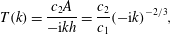
 $$\begin{eqnarray}\displaystyle & -\unicode[STIX]{x1D713}^{\prime }(0)=(-\text{i}k)^{-1/3}c_{1}A=h, & \displaystyle\end{eqnarray}$$
 $$\begin{eqnarray}\displaystyle & T(k)=\displaystyle \frac{c_{2}A}{-\text{i}kh}=\frac{c_{2}}{c_{1}}(-\text{i}k)^{-2/3}, & \displaystyle\end{eqnarray}$$
where
 $$\begin{eqnarray}\displaystyle & \displaystyle \frac{c_{2}}{c_{1}}=3^{1/3}/\unicode[STIX]{x0393}(2/3)\approx 1.06508, & \displaystyle\end{eqnarray}$$
i.e. a transfer function whose modulus decreases with
 $k$
as
 $k^{-2/3}$
. It should be remarked that the generally complex function
 $T(k)$
must be the Fourier transform of a real function of
 $x$
, and therefore must have symmetric real and antisymmetric imaginary part. This symmetry uniquely determines its behaviour for negative
 $k$
and therefore the correct branch of the polydromic function (3.14). As noted below (3.11), the correct branch is the one that is real and positive for
 $-\text{i}k$
real and positive. Its inverse Fourier transform, the spatial response produced by an infinitesimal step in
 $h(x)$
, is
 $$\begin{eqnarray}\displaystyle t(x)=\left\{\begin{array}{@{}ll@{}}0 & \text{for }x\leqslant 0\\ \displaystyle \frac{3^{1/3}}{\unicode[STIX]{x0393}^{2}(2/3)}\,x^{-1/3}\approx 0.78655\,x^{-1/3} & \text{for }x>0.\end{array}\right. & & \displaystyle\end{eqnarray}$$
As an additional remark, as long as the admittance of the outer flow is negligible, details of the velocity profile other than its derivative at zero have no leading-order role in the expression of the wall shear stress, nor does the boundary-layer thickness or its corresponding Reynolds number appear in it. For confined flow this will turn out to be the case up until regime 3 is entered.
3.2.2 Regime 2:
$Y=\infty$

According to (3.11), the ratio
 $\text{i}k\unicode[STIX]{x1D713}/p$
is proportional to both
 $z$
and
 $k$
. Therefore, with decreasing
 $k$
, a regime may eventually be entered in which at the height
 $z\simeq \unicode[STIX]{x1D6FF}$
this ratio drops below the admittance
 $Y$
of the outer flow. Here a distinction must be made between confined and open flow: confined flow obstructs normal velocity owing to the presence of the opposing wall; it has virtually zero admittance, and therefore the
 $Y=0$
regime can be expected to continue to much smaller
 $k$
than for open flow; on the other hand, an open boundary layer classically tracks the pressure of the outer flow and in return imposes a normal velocity as a higher-order perturbation upon it. In other words, a classical boundary layer obeying the theory of matched asymptotic expansions faces an infinite admittance at its edge.
In order to attain an expression of the shear-stress transfer function, the infinite-admittance regime must be handled in two successive approximations. At leading order there is no perturbation and no pressure in the outer flow; the solution of (3.8) for
 $p=0$
is (3.11) with
 $A=p=0$
and
 $B=-h$
. At this order of approximation there is no pressure or shear stress on the wall either. However, there is a normal velocity
 $v=\text{i}k\unicode[STIX]{x1D713}=-\text{i}khz$
induced at the upper edge of the boundary layer, which in the approximate Rayleigh region (3.4) becomes
 $v=-\text{i}khU$
and therefore in the potential region
 $v=-\text{i}khU_{ext}$
. It can be remarked that this is also the normal velocity that would be seen by imposing the linearized boundary condition (3.7) on the inviscid flow directly. Its corresponding irrotational solution (3.6) is
 $\unicode[STIX]{x1D713}=-hU_{ext}\exp (-|k|z)$
, and produces a pressure
 $p=-U_{ext}\unicode[STIX]{x1D713}^{\prime }(0)=-U_{ext}^{2}|k|h$
.
Reinjecting this pressure into the boundary-layer solution (3.11) yields, at the next order of approximation,
 $$\begin{eqnarray}\displaystyle & \unicode[STIX]{x1D713}(0)=(-\text{i}k)^{-2/3}c_{0}A-|k|hU_{ext}^{2}=0, & \displaystyle\end{eqnarray}$$
 $$\begin{eqnarray}\displaystyle & T(k)=\displaystyle \frac{c_{2}A}{-\text{i}kh}=U_{ext}^{2}\frac{c_{2}}{c_{0}}\text{i}\,\text{sign}(k)(-\text{i}k)^{2/3}, & \displaystyle\end{eqnarray}$$
where
 $$\begin{eqnarray}\displaystyle \displaystyle \frac{c_{2}}{c_{0}} & = & \displaystyle \frac{3^{-1/3}\unicode[STIX]{x0393}(1/3)}{\unicode[STIX]{x0393}(2/3)}\approx 1.37172.\end{eqnarray}$$
Therefore, in the infinite-admittance regime the shear-stress spectral response
 $T(k)$
is now proportional to
 $k^{+2/3}$
, as opposed to
 $k^{-2/3}$
in the zero-admittance regime. In addition, owing to the presence of the sign function, (3.18) is not an analytic function in either the half-plane
 $\text{real}(-\text{i}k)>0$
or
 $\text{real}(-\text{i}k)<0$
, which means that the physical-domain response function is different from zero in both
 $x>0$
and
 $x<0$
, as may be expected to occur under the influence of the elliptic potential flow.
3.2.3 Finite admittance: the interacting boundary layer
The amplitudes of (3.14) and (3.18) become comparable to each other when
 $k^{4/3}U_{ext}^{2}\simeq 1$
; that is, upon considering that in a laminar boundary layer
 $U_{ext}\simeq \text{Re}_{\unicode[STIX]{x1D70F}}$
, they become comparable when
 $k\simeq \text{Re}_{\unicode[STIX]{x1D70F}}^{-3/2}$
. This is the wavenumber threshold where the transfer function can be expected to shift from regime 1 to regime 2. Interestingly it occurs in a range where already
 $k\unicode[STIX]{x1D6FF}=k\text{Re}_{\unicode[STIX]{x1D70F}}\ll 1$
, a condition which will allow further simplifications.
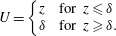
In order to start with an example that allows a simpler solution, we can consider a piecewise-linear base velocity profile,
 $$\begin{eqnarray}\displaystyle U=\left\{\begin{array}{@{}cl@{}}z & \text{for }z\leqslant \unicode[STIX]{x1D6FF}\\ \unicode[STIX]{x1D6FF} & \text{for }z\geqslant \unicode[STIX]{x1D6FF}.\end{array}\right. & & \displaystyle\end{eqnarray}$$
In this example the exact Couette-flow solution (3.11) applies for all
 $z\leqslant \unicode[STIX]{x1D6FF}=U_{ext}=\text{Re}_{\unicode[STIX]{x1D70F}}$
, whereas for
 $z\geqslant \unicode[STIX]{x1D6FF}$
the potential equation (3.5) provides the solution
 $\unicode[STIX]{x1D713}(z)=\unicode[STIX]{x1D713}(\unicode[STIX]{x1D6FF})\exp [-|k|(z-\unicode[STIX]{x1D6FF})]$
,
 $p(z)=-U_{ext}\unicode[STIX]{x1D713}^{\prime }(z)$
.
At
 $z=\unicode[STIX]{x1D6FF}$
,
 $\unicode[STIX]{x1D713}^{\prime }$
is discontinuous just like
 $U^{\prime }$
is, but
 $U\unicode[STIX]{x1D713}^{\prime }-U^{\prime }\unicode[STIX]{x1D713}=-p$
is continuous. Therefore the potential admittance condition
 $\unicode[STIX]{x1D713}^{\prime }(\unicode[STIX]{x1D6FF}+)=-|k|\unicode[STIX]{x1D713}(\unicode[STIX]{x1D6FF})$
becomes, immediately to the left of
 $z=\unicode[STIX]{x1D6FF}$
,
 $\unicode[STIX]{x1D713}^{\prime }(\unicode[STIX]{x1D6FF}-)=[U_{ext}^{-1}-|k|]\unicode[STIX]{x1D713}(\unicode[STIX]{x1D6FF})$
, with
 $p(\unicode[STIX]{x1D6FF}-)=p(\unicode[STIX]{x1D6FF}+)=U_{ext}|k|\unicode[STIX]{x1D713}(\unicode[STIX]{x1D6FF})$
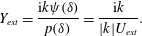
. The admittance
 $Y(z)$
is continuous (but with discontinuous derivative) at
 $z=\unicode[STIX]{x1D6FF}$
, and it equals
 $$\begin{eqnarray}Y_{ext}=\frac{\text{i}k\unicode[STIX]{x1D713}(\unicode[STIX]{x1D6FF})}{p(\unicode[STIX]{x1D6FF})}=\frac{\text{i}k}{|k|U_{ext}}.\end{eqnarray}$$
For
 $z<\unicode[STIX]{x1D6FF}$
it is given by
 $$\begin{eqnarray}Y(z)=\frac{\text{i}k\unicode[STIX]{x1D713}(z)}{p(z)}=\text{i}k+\text{i}k\left(\frac{1}{|k|U_{ext}^{2}}-\frac{1}{\unicode[STIX]{x1D6FF}}\right)z.\end{eqnarray}$$
The term
 $1/\unicode[STIX]{x1D6FF}$
is of a higher order with respect to
 $1/(|k|U_{ext}^{2})$
, since
 $\unicode[STIX]{x1D6FF}=U_{ext}$
and, in the distinguished limit of
 $k=O(\unicode[STIX]{x1D6FF}^{-3/2})$
,
 $k\unicode[STIX]{x1D6FF}\rightarrow 0$
when
 $\unicode[STIX]{x1D6FF}\rightarrow \infty$
. Comparing (3.22) with (3.11) for large
 $z$
provides
 $B=(|k|U_{ext}^{2})^{-1}p$
; (3.12) inserted into the boundary conditions (2.2) then give
 $$\begin{eqnarray}\displaystyle (-\text{i}k)^{-2/3}c_{0}A+p=0,\quad B-(-\text{i}k)^{-1/3}c_{1}A=-h, & & \displaystyle\end{eqnarray}$$
 $$\begin{eqnarray}\displaystyle T(k)=c_{2}A/(-\text{i}kh) & & \displaystyle\end{eqnarray}$$
whence, by elimination,
 $[(-\text{i}k)^{-1/3}c_{1}+(|k|U_{ext}^{2})^{-1}(-\text{i}k)^{-2/3}c_{0}]A=h$
and
 $$\begin{eqnarray}T(k)=[(c_{1}/c_{2})(-\text{i}k)^{2/3}-\text{i}(c_{0}/c_{2})U_{ext}^{-2}(-\text{i}k)^{-2/3}\,\text{sign}(k)]^{-1},\end{eqnarray}$$
with
 $c_{1}/c_{2}=3^{-1/3}\unicode[STIX]{x0393}(2/3)\approx 0.93889$
and
 $c_{0}/c_{2}=3^{1/3}\unicode[STIX]{x0393}(2/3)/\unicode[STIX]{x0393}(1/3)\approx 0.72901$
.
This leading-order solution, obtained for a piecewise-linear velocity profile, actually turns out to be the correct expression of
 $T(k)$
in the general case of an arbitrary velocity profile, because, as will now be seen, the shape of the profile only entails higher-order corrections. Let us consider the case where the linear region
 $U(z)=z$
, instead of becoming abruptly constant at
 $z=\unicode[STIX]{x1D6FF}$
, is joined to the constant region
 $U(z)=U_{ext}$
by a smooth curve extending from an inner point
 $z_{1}<\unicode[STIX]{x1D6FF}$
to an outer point
 $z_{2}>\unicode[STIX]{x1D6FF}$
, with both nonetheless
 $O(\unicode[STIX]{x1D6FF})$
. Between
 $z_{1}$
and
 $z_{2}$
the approximate solution (3.4) of the Rayleigh equation is valid; imposing at
 $z=z_{2}$
the potential admittance condition
 $\unicode[STIX]{x1D713}^{\prime }(z_{2})=-|k|\unicode[STIX]{x1D713}(z_{2})$
, we obtain
 $$\begin{eqnarray}\displaystyle Y(z)=\frac{\text{i}k\unicode[STIX]{x1D713}(z)}{p}=-\text{i}kU(z)\left[\int _{z}^{z_{2}}U^{-2}\,\text{d}z-\frac{1}{|k|U_{ext}^{2}}\right]. & & \displaystyle\end{eqnarray}$$
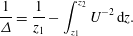
For
 $z\leqslant z_{1}$
, where
 $U(z)\approx z$
, this may be rewritten as
 $$\begin{eqnarray}Y(z)=\text{i}k+\text{i}k\left(\frac{1}{|k|U_{ext}^{2}}-\frac{1}{\unicode[STIX]{x1D6E5}}\right)z,\end{eqnarray}$$
where
 $$\begin{eqnarray}\frac{1}{\unicode[STIX]{x1D6E5}}=\frac{1}{z_{1}}-\int _{z_{1}}^{z_{2}}U^{-2}\,\text{d}z.\end{eqnarray}$$
Whatever the shape of the velocity profile,
 $\unicode[STIX]{x1D6E5}$
is of the same order as
 $\unicode[STIX]{x1D6FF}\simeq U_{ext}$
, and therefore in (3.26)
 $1/\unicode[STIX]{x1D6E5}$
is vanishing with respect to
 $1/(|k|U_{ext}^{2})$
when
 $|k|\unicode[STIX]{x1D6FF}\rightarrow 0$
just as
 $1/\unicode[STIX]{x1D6FF}$
was in (3.22). The difference between (3.26) and (3.22) is therefore negligible in this limit. In fact (3.27) can also be taken to the limit for
 $z_{1}\rightarrow 0$
, when
 $U^{\prime \prime }(0)=0$
, without changing this estimate. When the second derivative
 $U^{\prime \prime }(0)\neq 0$
, that is when the base flow has its own non-zero pressure gradient, the limit for
 $z_{1}\rightarrow 0$
of (3.27) diverges, but this divergence can be circumvented by the method of Tollmien (Reference Tollmien1929). This modification again leaves the present leading-order estimate (3.24) unchanged. In conclusion, the transfer function (3.24) represents the union of regimes 1 and 2 at leading order for an arbitrary velocity profile.
3.3 Regime 3: fully developed flow
In the case of confined flow, the fully developed perturbed flow is the local Poiseuille flow in a channel of modified half-height
 $\unicode[STIX]{x1D6FF}-h(x)$
. For a varicose perturbation, where
 $z=\unicode[STIX]{x1D6FF}$
is a symmetry plane, the centreline velocity goes from
 $U_{ext}=0.5\unicode[STIX]{x1D6FF}$
to
 $U_{ext}=0.5\unicode[STIX]{x1D6FF}/(1-h(x)/\unicode[STIX]{x1D6FF})$
owing to mass conservation, and the skin friction from
 $1$
to
 $(1-h(x)/\unicode[STIX]{x1D6FF})^{-2}\simeq 1+2h(x)/\unicode[STIX]{x1D6FF}$
. In Fourier space, the corresponding transfer function is
 $T(k)=2\text{i}/(k\unicode[STIX]{x1D6FF})$
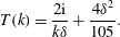
. An expansion of
 $T(k)$
in powers of
 $k$
up to the next order was calculated by Benjamin (Reference Benjamin1957) and by Luchini & Charru (Reference Luchini and Charru2010); in the present non-dimensionalization it can be written as
 $$\begin{eqnarray}T(k)=\frac{2\text{i}}{k\unicode[STIX]{x1D6FF}}+\frac{4\unicode[STIX]{x1D6FF}^{2}}{105}.\end{eqnarray}$$
This fully developed regime is achieved when the viscous length
 $k^{-1/3}$
becomes larger than the channel half-width
 $\unicode[STIX]{x1D6FF}$
, that is when
 $k\ll \unicode[STIX]{x1D6FF}^{-3}$
. For the whole interval
 $\unicode[STIX]{x1D6FF}^{-3}\ll k\ll 1$
a confined flow remains in the zero-admittance regime 1, governed by the friction transfer function (3.14). It can easily be verified that
 $k\simeq \unicode[STIX]{x1D6FF}^{-3}$
is the value where the orders of magnitude of (3.14) and (3.28) cross each other. (An attentive eye will notice that the real and imaginary parts of
 $T(k)$
switch regimes at almost two decades’ distance in
 $k$
, owing to the appearance of the small factor
 $4/105$
in (3.28); but the same asymptotic scaling is respected for both.)
For open flow one might a priori expect that a similar quasi-one-dimensional regime could be attained for small enough
 $k$
, a regime where the main contribution to
 $T(k)$
is proportional to the inviscid longitudinal velocity perturbation. The resulting shear-stress transfer function would be
 $$\begin{eqnarray}T(k)=|k|/(-\text{i}k)=\text{i}\,\text{sign}(k).\end{eqnarray}$$
However, the wavenumber
 $k\simeq \unicode[STIX]{x1D6FF}^{-3}$
where this may be expected to happen also has another special meaning. A boundary layer grows to a thickness
 $\unicode[STIX]{x1D6FF}_{dim}\simeq \sqrt{L_{dim}\unicode[STIX]{x1D708}_{dim}/U_{ext,dim}}$
after a distance
 $L_{dim}$
from its origin. Reversing the argument, a boundary layer of thickness
 $\unicode[STIX]{x1D6FF}_{dim}$
must have originated at a distance not larger than
 $L_{dim}=\unicode[STIX]{x1D6FF}_{dim}^{2}U_{ext,dim}/\unicode[STIX]{x1D708}_{dim}$
upstream of the point where it is measured. Wavelengths larger than
 $L_{dim}$
have no meaning, even more so in a locally parallel approximation: they would imply an oscillation over a length larger than the boundary layer itself. When non-dimensionalized in viscous units, the development distance from the leading edge becomes
 $L=\unicode[STIX]{x1D6FF}^{3}$
, and therefore the fully developed range of the shear-stress transfer function, if there existed one for open flow, would be composed of wavelengths exceeding this upper bound. This range is marked ‘impossible’ in table 1.
4 Numerical solution: what happened to regime 2?
Elegant as the asymptotic techniques are, eventually they are nothing else than an approximate solution of the Orr–Sommerfeld equation (2.1), or at least so we are induced to believe by the way they were derived. The Orr–Sommerfeld equation can just as well be solved numerically, and while this path was barely beginning to be explored in Benjamin’s time, today it is nearly a classroom exercise. In doing so, however, a surprise awaits us.
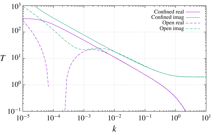
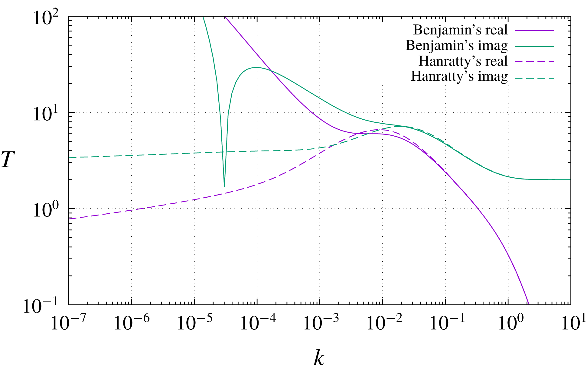
Figure 2 displays the shear-stress transfer function, as previously defined in (2.5), as a function of wavenumber
 $k$
for confined Poiseuille flow at
 $\unicode[STIX]{x1D6FF}=\text{Re}_{\unicode[STIX]{x1D70F}}=100$
, which translates into
 $\text{Re}_{\unicode[STIX]{x1D6FF}}=\unicode[STIX]{x1D6FF}_{dim}U_{ext,dim}/\unicode[STIX]{x1D708}_{dim}=\text{Re}_{\unicode[STIX]{x1D70F}}^{2}/2=5000$
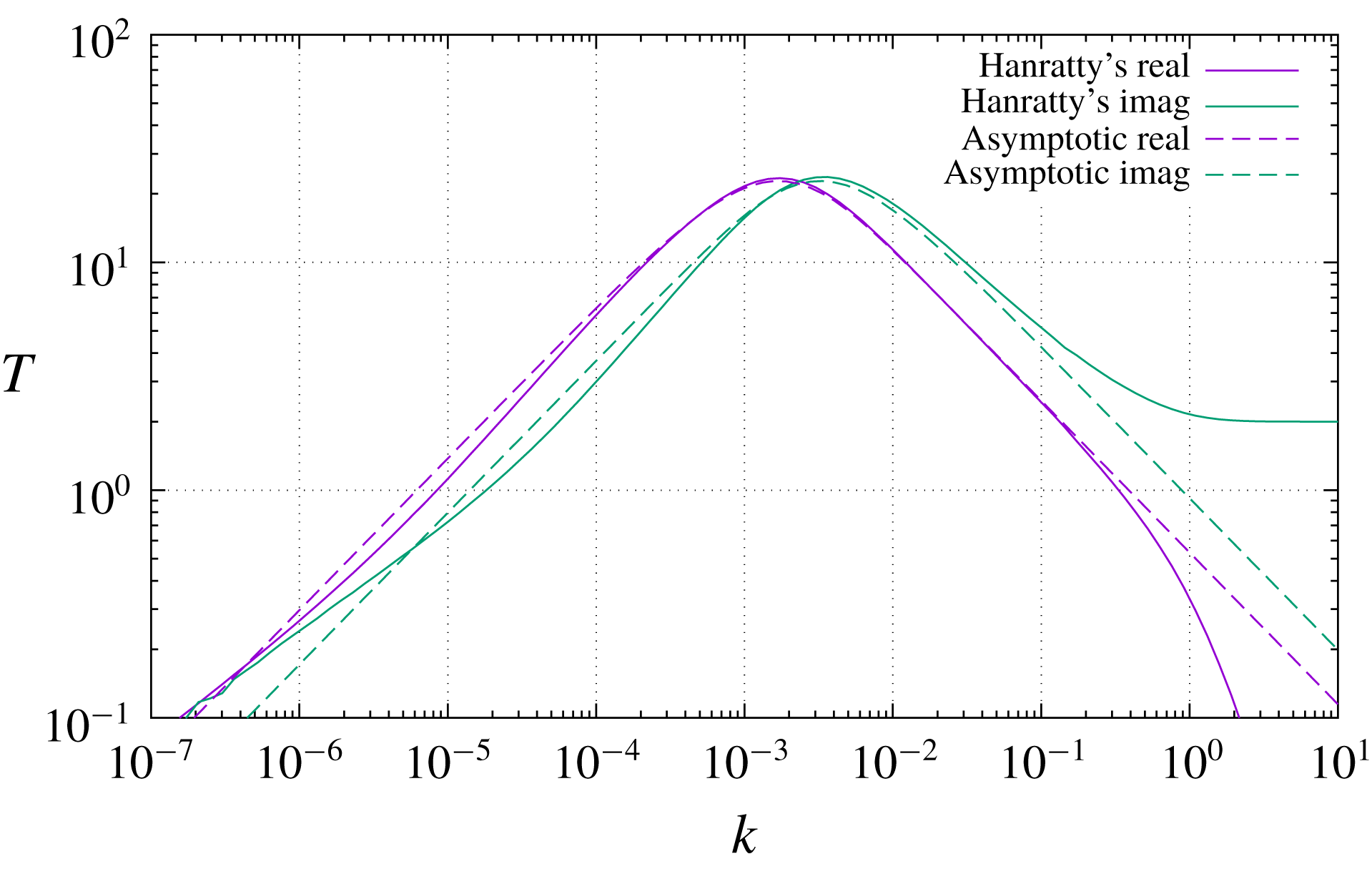
. The three regimes 0, 1 and 3 foreseen by the asymptotic analysis are clearly visible, with no trace of regime 2 which confirms that for confined flow, admittance is always vanishing because of the blockage effect of the opposing wall.
Confined Poiseuille flow and open boundary layer at
 $\text{Re}_{\unicode[STIX]{x1D70F}}=100$
, or
 $\text{Re}_{\unicode[STIX]{x1D6FF}}=5000$
.
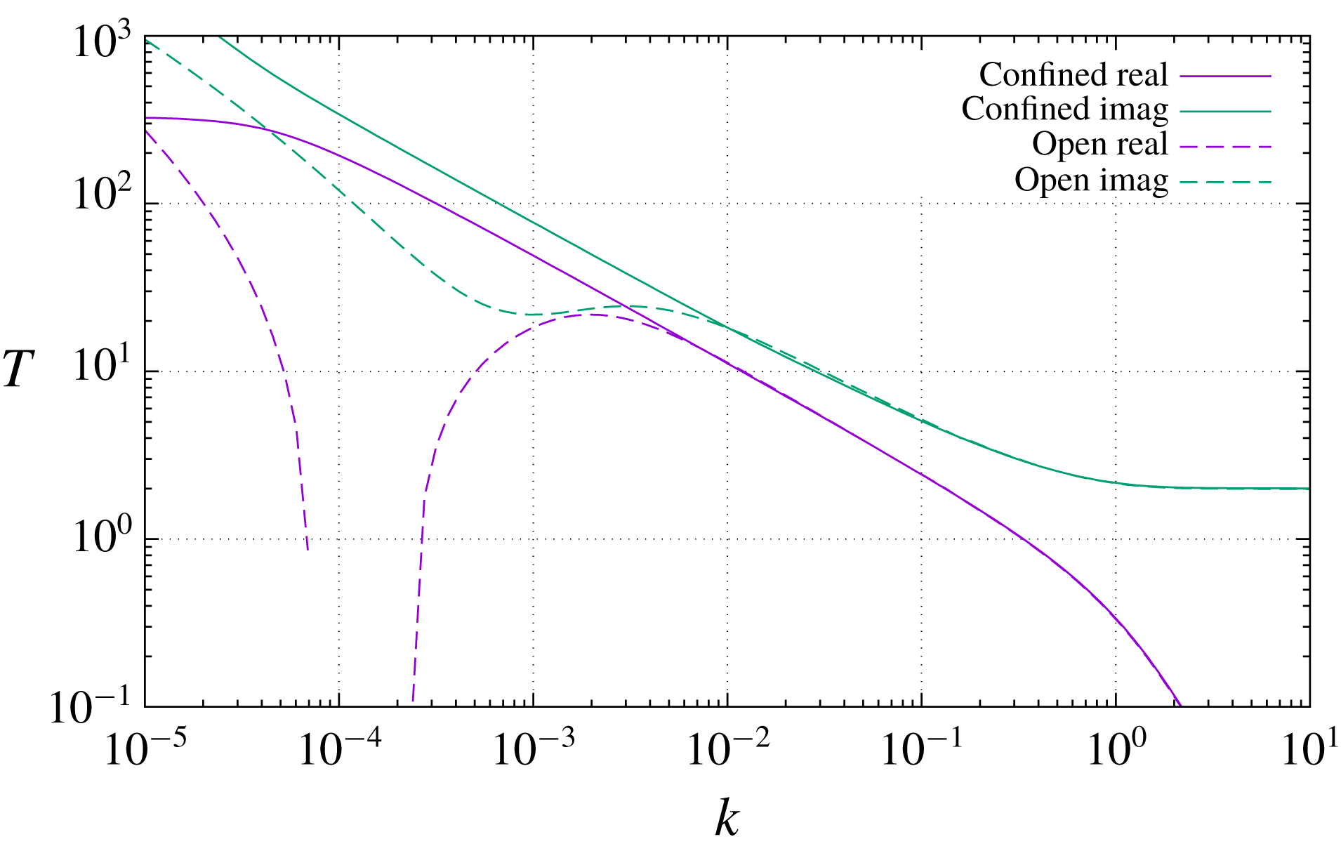
The same figure 2 also displays a similar transfer-function plot for a laminar boundary layer at
 $\text{Re}_{\unicode[STIX]{x1D70F}}=100$
(
 $\text{Re}_{L}\approx 10^{6}$
). Here we expect to see all four regimes 0, 1, 2, 3. But, to our own great surprise when we first saw this plot, we do not. All is well for
 $k\gtrsim \unicode[STIX]{x1D6FF}^{-3/2}$
, which for this Reynolds number is
 $k\gtrsim 10^{-3}$
; there we see the
 $k^{-2/3}$
slope characterizing regime 1 followed by the signature of regime 0. But, despite a very shallow local maximum appears in the neighbourhood of
 $k\simeq \unicode[STIX]{x1D6FF}^{-3/2}$
, about where we expect it, there is no evidence of a
 $k^{2/3}$
behaviour at its left. (Incidentally, the dip visible in the real part is an artefact of the logarithmic scale, since the curve crosses zero and then diverges on the negative side.) We verified the numerical solution extensively, but there is not much that can go wrong with it. The Orr–Sommerfeld equation and its own asymptotic approximation were being inconsistent.
5 Loss of the Prandtl invariance and its recovery
Despite the fact that the Orr–Sommerfeld equation (2.1) was initially derived by Benjamin in a curvilinear reference frame, it can be remarked that
 $\unicode[STIX]{x1D713}$
is the original perturbation streamfunction as defined in the Cartesian frame, and (2.1) and its boundary conditions (2.2) are identical to those that can be derived by linearizing the Cartesian Navier–Stokes equations directly about a parallel flow with no change of frame. Therefore, Benjamin’s derivation can be seen as a theoretical justification for the latter procedure.
In contrast, Hanratty and coworkers (Thorsness et al.
Reference Thorsness, Morrisroe and Hanratty1978), having in mind the application of mixing-length turbulence models in which eddy viscosity is a function of distance from the actual wall, introduced a boundary-layer coordinate system in which the normal coordinate is such distance. They wrote the following equation for the streamfunction
 $\unicode[STIX]{x1D713}_{rel}$
in this relative (to the wall) coordinate system:
 $$\begin{eqnarray}-\text{i}k(U\unicode[STIX]{x1D713}_{rel}^{\prime \prime }-U^{\prime \prime }\unicode[STIX]{x1D713}_{rel}-k^{2}U\unicode[STIX]{x1D713}_{rel}+k^{2}hU^{2})=k^{4}\unicode[STIX]{x1D713}_{rel}-2k^{2}\unicode[STIX]{x1D713}_{rel}^{\prime \prime }+\unicode[STIX]{x1D713}_{rel}^{\prime \prime \prime \prime }-k^{4}hU+2k^{2}hU^{\prime \prime },\end{eqnarray}$$
which differs from Benjamin’s in two fundamental ways: the presence of the ‘centripetal force’ term
 $-\text{i}k^{3}hU^{2}$
, and the fact that
 $\unicode[STIX]{x1D713}_{rel}$
is the perturbation streamfunction relative to the displaced wall, i.e. deprived of the rigid displacement
 $\unicode[STIX]{x1D713}=-hU$
. In addition (11) of Thorsness et al. (Reference Thorsness, Morrisroe and Hanratty1978) contains curvature-modified Reynolds stresses whose description will be delayed to § 7.3, since we wish to only discuss laminar flow in the present section.
As remarked by Thorsness et al. (Reference Thorsness, Morrisroe and Hanratty1978), equation (5.1) can also be reformulated in the original Cartesian coordinate system by the change of variables
 $\unicode[STIX]{x1D713}_{rel}=\unicode[STIX]{x1D713}+hU$
, with the result that
 $$\begin{eqnarray}-\text{i}k(U\unicode[STIX]{x1D713}^{\prime \prime }-U^{\prime \prime }\unicode[STIX]{x1D713}-k^{2}U\unicode[STIX]{x1D713})=k^{4}\unicode[STIX]{x1D713}-2k^{2}\unicode[STIX]{x1D713}^{\prime \prime }+\unicode[STIX]{x1D713}^{\prime \prime \prime \prime }+hU^{\prime \prime \prime \prime }.\end{eqnarray}$$
Thorsness et al. (Reference Thorsness, Morrisroe and Hanratty1978) ascribe the difference between their and Benjamin’s formulation to the appearance of
 $U^{\prime \prime \prime \prime }$
in the viscous term on the right side of (5.7), which results from the inclusion of a centripetal acceleration term in (5.1). They then proceed to explore turbulence models and the effects of curvature upon them. Although the same equation eventually springs out of the derivation below, our interpretation will be somewhat different. In fact, as will be seen from the numerical results, even in the laminar regime the largest difference between Benjamin’s and Hanratty’s formulation arises in the limit of very small
 $k$
, where centripetal acceleration should be negligible.
A comparison of the boundary-layer approximation (3.2) of (2.1) with the classical, nonlinear and non-parallel boundary-layer equation highlights an incongruence. In viscous-unit scaling, the complete nonlinear boundary-layer equation reads
 $$\begin{eqnarray}\unicode[STIX]{x1D6F9}_{z}\unicode[STIX]{x1D6F9}_{xz}-\unicode[STIX]{x1D6F9}_{x}\unicode[STIX]{x1D6F9}_{zz}+P_{x}=\unicode[STIX]{x1D6F9}_{zzz}.\end{eqnarray}$$
As is easily verified, a change of independent variable from
 $z$
to
 $\unicode[STIX]{x1D701}=z-h(x)$
leaves this equation unchanged, for arbitrary
 $h(x)$
, and the same is true of the boundary conditions
 $\unicode[STIX]{x1D6F9}=\unicode[STIX]{x1D6F9}_{z}=0$
if applied at the new wall position
 $z=h(x)$
. In words, if
 $\unicode[STIX]{x1D6F9}(x,z)$
is a known solution (for an arbitrary pressure gradient) of (5.3) over a plane wall,
 $\unicode[STIX]{x1D6F9}(x,z-h(x))$
is the exact solution of (5.3) over a wall located at
 $z=h(x)$
. This is known as Prandtl’s displacement invariance property. If now (5.3) is linearized for a streamfunction perturbation
 $\unicode[STIX]{x1D713}$
,
 $$\begin{eqnarray}\unicode[STIX]{x1D6F9}_{z}\unicode[STIX]{x1D713}_{xz}-\unicode[STIX]{x1D6F9}_{zz}\unicode[STIX]{x1D713}_{x}+\underbrace{\unicode[STIX]{x1D6F9}_{xz}\unicode[STIX]{x1D713}_{z}-\unicode[STIX]{x1D6F9}_{x}\unicode[STIX]{x1D713}_{zz}}_{\mathit{non-parallel\,terms}}+p_{x}=\unicode[STIX]{x1D713}_{zzz},\end{eqnarray}$$
it can easily be verified that a linearized version of the same invariance property still holds; in particular
 $\unicode[STIX]{x1D713}=-hU$
, the first term in a Taylor expansion of
 $\unicode[STIX]{x1D6F9}(x,z-h(x))$
with
 $U=\unicode[STIX]{x1D6F9}_{z}$
, is always an exact solution of (5.4) and the appropriate boundary conditions (2.2). Incidentally, it follows from this property that a wall perturbation
 $h(x)$
translates into
 $\unicode[STIX]{x1D713}=-hU_{ext}$
and
 $v=-\unicode[STIX]{x1D713}_{x}=U_{ext}h_{x}$
at the edge of the boundary layer, that is, quite naturally, into the standard boundary condition that applies to an inviscid flow when the boundary-layer thickness tends to zero.
On the other hand, if the non-parallel terms
 $\unicode[STIX]{x1D6F9}_{xz}\unicode[STIX]{x1D713}_{z}-\unicode[STIX]{x1D6F9}_{x}\unicode[STIX]{x1D713}_{zz}$
are neglected in (5.4), the above property is no longer exact;
 $\unicode[STIX]{x1D713}=-hU$
is not a solution of (3.2), the boundary-layer limiting form of the intrinsically parallel Orr–Sommerfeld equation, which lacks just such non-parallel terms. With parallelization, Prandtl’s displacement invariance symmetry is broken; hence, Benjamin’s curvilinear-coordinates formulation and the original Cartesian formulation are no longer equivalent as we were led to believe.
Keeping all the non-parallel terms that Benjamin had decided to neglect would make the problem intractable, in addition to making it dependent on the
 $x$
derivatives of the base flow which may not be easily available. But as we shall show through examples, Thorsness et al.’s (Reference Thorsness, Morrisroe and Hanratty1978) modification to the original problem (2.1) can actually solve the issue. If the streamfunction is parallelized about the partially perturbed flow
 $\unicode[STIX]{x1D6F9}(x,z)-h(x)U(x,z)$
, rather than about the original
 $\unicode[STIX]{x1D6F9}(x,z)$
, the new perturbation streamfunction
 $\unicode[STIX]{x1D713}_{rel}=\unicode[STIX]{x1D713}+hU$
, according to Prandtl’s invariance property obeys an
 $x$
-dependent boundary-layer equation identical to the one
 $\unicode[STIX]{x1D713}$
does, but the parallel approximations (3.2a
) of one and the other equation are not equivalent to each other. Let us write (3.2a
) for
 $\unicode[STIX]{x1D713}_{rel}$
as
 $$\begin{eqnarray}\displaystyle -\text{i}k(U\unicode[STIX]{x1D713}_{rel}^{\prime }-U^{\prime }\unicode[STIX]{x1D713}_{rel}+p)=\unicode[STIX]{x1D713}_{rel}^{\prime \prime \prime }, & & \displaystyle\end{eqnarray}$$
and then revert to
 $\unicode[STIX]{x1D713}$
through the substitution
 $\unicode[STIX]{x1D713}_{rel}=\unicode[STIX]{x1D713}+hU$
. The result is
 $$\begin{eqnarray}-\text{i}k(U\unicode[STIX]{x1D713}^{\prime }-U^{\prime }\unicode[STIX]{x1D713}+p)=\unicode[STIX]{x1D713}^{\prime \prime \prime }+hU^{\prime \prime \prime },\end{eqnarray}$$
with an additional term with respect to the former equation (3.2a
). Because of the underlying boundary-layer equation obeyed by the base flow, this inhomogeneous term
 $hU^{\prime \prime \prime }$
, despite containing no
 $x$
derivative, approximately equals and replaces contributions of the form
 $\unicode[STIX]{x1D6F9}_{xz}\unicode[STIX]{x1D713}_{z}-\unicode[STIX]{x1D6F9}_{x}\unicode[STIX]{x1D713}_{zz}$
which would appear in the linearized, non-parallel boundary-layer equations. In practice it restores
 $\unicode[STIX]{x1D713}=-hU$
as one of the exact solutions of (5.6), as is easily verified. In addition, the third derivative
 $hU^{\prime \prime \prime }$
goes quickly to zero outside the boundary layer, thus it does no harm to include it everywhere. This implies that the Orr–Sommerfeld equation (2.1) modifies with an additional inhomogeneous term into
 $$\begin{eqnarray}-\text{i}k(U\unicode[STIX]{x1D713}^{\prime \prime }-U^{\prime \prime }\unicode[STIX]{x1D713}-k^{2}U\unicode[STIX]{x1D713})=k^{4}\unicode[STIX]{x1D713}-2k^{2}\unicode[STIX]{x1D713}^{\prime \prime }+\unicode[STIX]{x1D713}^{\prime \prime \prime \prime }+hU^{\prime \prime \prime \prime }.\end{eqnarray}$$
Together with the unmodified boundary conditions (2.2), (5.7) provides a uniformly valid parallel approximation which tends to the invariant limiting form (5.6) in the boundary layer and to its original form (2.1) elsewhere. This can be recognized to be the same as Hanratty’s equation (5.2), and was used by Hanratty and coworkers in several articles (Zilker et al. Reference Zilker, Cook and Hanratty1977; Thorsness et al. Reference Thorsness, Morrisroe and Hanratty1978; Abrams & Hanratty Reference Abrams and Hanratty1985) where they compared its turbulent-flow numerical solutions with their experiments.
From an alternate viewpoint one can conceive an unperturbed boundary layer, over a wall in the reference position
 $z=0$
, which is held exactly parallel by a real or fictitious external force
 $F(z)$
. For this to happen,
 $F(z)$
must exactly balance diffusion: in dimensionless form,
 $F(z)+U^{\prime \prime }(z)=0$
. For the perturbed problem with a wall located at
 $z=h(x)$
, depending on the physical nature of
 $F$
, this force may stay in its original position or, more likely, be convected with the wall and thus become
 $F[z-h(x)]$
(the second is especially the case if
 $F$
is considered to be a fictitious force mimicking the inertial action of the flow itself). A Taylor expansion with respect to
 $h$
now produces a linearized force
 $-hF^{\prime }(z)=hU^{\prime \prime \prime }(z)$
, and in the Orr–Sommerfeld equation its derivative
 $hU^{\prime \prime \prime \prime }(z)$
, which is exactly the innovation between Hanratty’s equation (5.7) and Benjamin’s equation (2.1). The advantage of this alternate derivation of (5.7) is that it does not in principle require that the boundary layer and inviscid region be formally distinguished from each other. As a side note it can be remarked that in the most obvious instance of parallel flow under the action of a physical volume force, Poiseuille flow under the action of either an external pressure gradient or gravity,
 $F(z)$
is constant and
 $U^{\prime \prime \prime }$
vanishes. But it does not vanish for a typical boundary layer.
Either way, we arrive at the same inhomogeneous Orr–Sommerfeld equation (5.7). The effect of this modification to restore Prandtl’s invariance will become apparent in the following numerical tests.
6 The numerical shear-stress transfer function
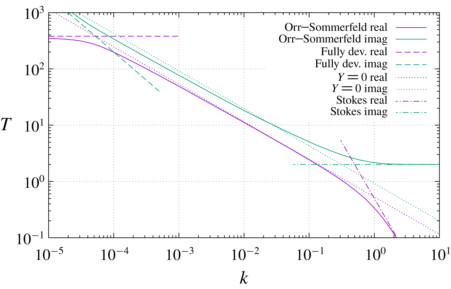
Figure 3 shows the shear-stress transfer function (2.5) as obtained from either Benjamin’s (2.1) or Hanratty’s (5.7) form of the Orr–Sommerfeld equation for confined Poiseuille flow. The two results are trivially identical because for a quadratic
 $U(z)$
, its third and fourth derivatives vanish. The same figure also displays the theoretical asymptotes characterizing the three regimes 0 (3.1), 1 (3.14) and 3 (3.28). There is no regime 2 anywhere in the spectrum for confined flow.

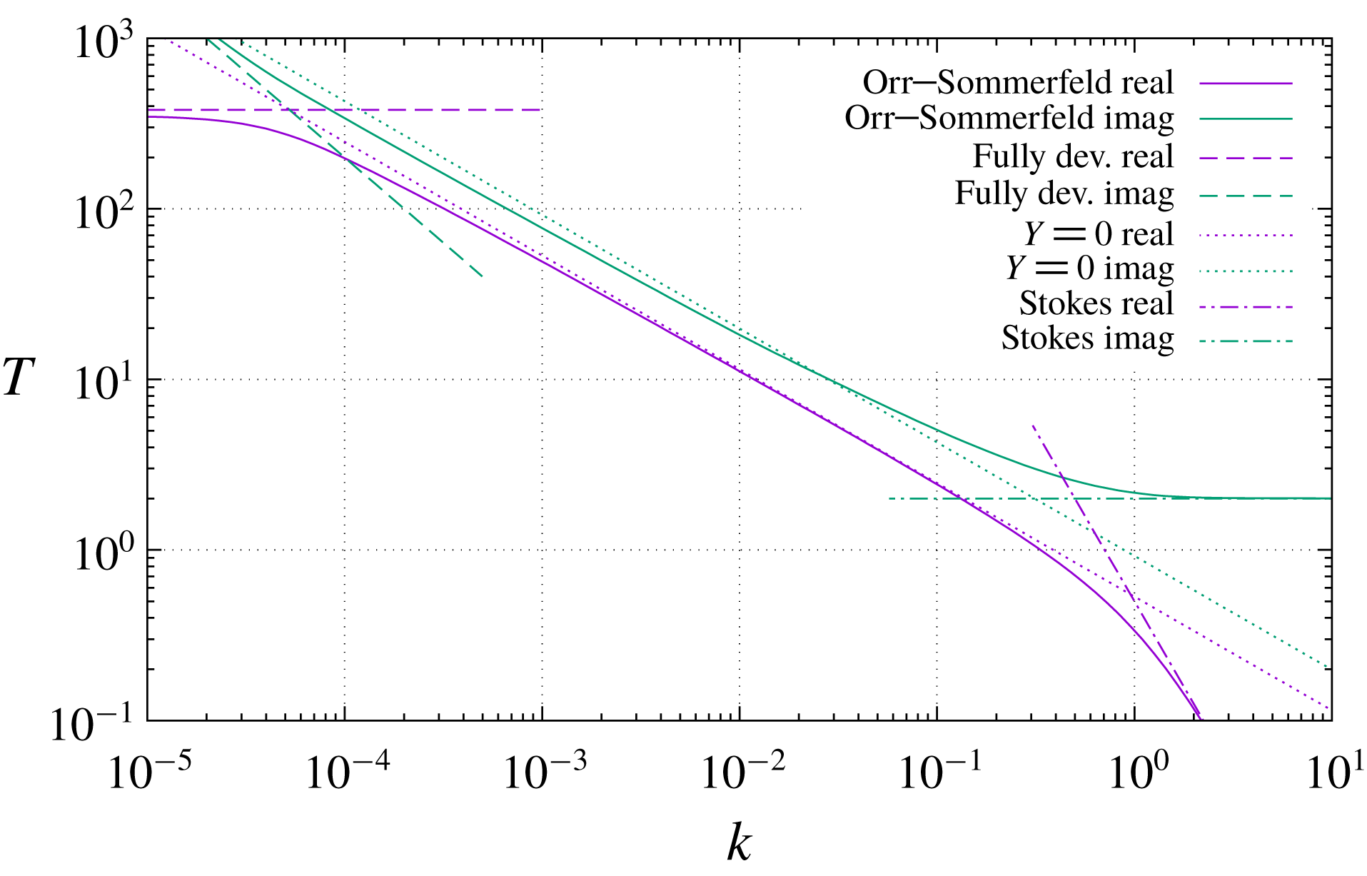

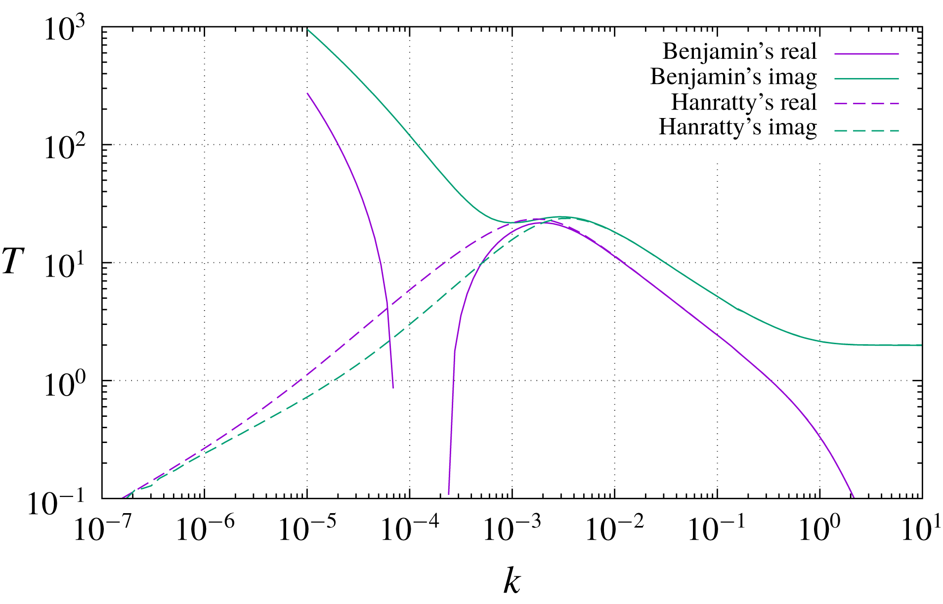
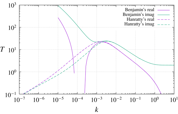
Figure 4 exhibits the shear-stress transfer function for a boundary-layer velocity profile, also at
 $\unicode[STIX]{x1D6FF}=\text{Re}_{\unicode[STIX]{x1D70F}}=100$
(with
 $\unicode[STIX]{x1D6FF}$
defined, for the present purposes, as
 $\unicode[STIX]{x1D6FF}=2U_{ext}$
, or
 $\unicode[STIX]{x1D6FF}_{dim}=2U_{ext,dim}/U_{dim}^{\prime }(0)$
, the same relationship that holds in the confined-flow example). Here the two curves coincide with each other (and at the same time with the corresponding curves for confined flow) to within the accuracy of the graph in the right half, corresponding to regimes 0 and 1 as described above, but in the left half of the graph the difference between Benjamin’s and Hanratty’s equation is dramatic. Whereas the numerical solution of (2.1), the same which was already seen in figure 2, fails to exhibit any regime 2 at all and keeps increasing (in modulus) left of
 $k\approx 2\times 10^{-3}$
, the solution of Hanratty’s equation (5.7) has a well evident maximum at about this value (slightly displaced between its real and imaginary parts) and then decreases with the expected
 $k^{2/3}$
slope to its left. The same behaviour is again observable in figure 5, where the solution of Hanratty’s equation (5.7) is compared to the asymptotic analytical solution (3.24). The agreement is remarkable, standing the simplicity of (3.24), and especially so in the proximity of the maximum response. The spectral range of maximum response is the most likely one to emerge in practical applications, just because wavenumbers where the transfer function is lower will be filtered out by the transfer function itself.

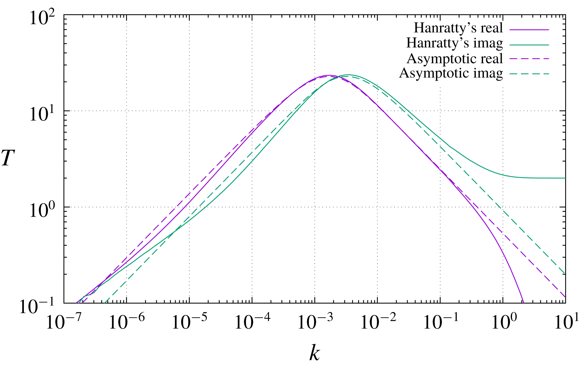
One may also observe from figure 5 that at approximately the same
 $k$
where confined flow attains its fully developed regime, the transfer function
 $T(k)$
of the boundary layer becomes of order unity, but for
 $k\ll \unicode[STIX]{x1D6FF}^{-3}$
, contrary to the prediction of (3.29), it keeps decreasing. This range is of little practical interest, because as was already remarked it corresponds to wavelengths longer than the boundary layer’s development length, but it is in principle attainable in an experiment in which the boundary layer is kept artificially parallel by an external force, such as an electric or perhaps thermal buoyancy force generated by the body surface. It is therefore of some interest to remark, from figure 5, that even in such an extreme case the hypothetical fully developed transfer function (3.29) is not achieved. The qualitative explanation of this failure is that now the boundary layer induced by the perturbation is even taller than the original one, and therefore the ratio between its induced shear stress and its outer velocity is not the same but smaller.
7 Turbulent flow
When the oncoming flow is turbulent, the equality
 $\unicode[STIX]{x1D6FF}=\text{Re}_{\unicode[STIX]{x1D70F}}$
remains true by definition, but the other approximate equality
 $U_{ext}\simeq \text{Re}_{\unicode[STIX]{x1D70F}}$
(a consequence in the laminar case of
 $U^{\prime }(0)=1$
and the presence of essentially a single length scale) changes dramatically to
 $U_{ext}\simeq \log (\text{Re}_{\unicode[STIX]{x1D70F}})$
. Many of the previous estimates must then be revised. In particular, the typical distance from the leading edge of an unperturbed boundary layer, which in the laminar case was
 $L\simeq \text{Re}_{\unicode[STIX]{x1D70F}}^{3}$
, is now
 $L\simeq \unicode[STIX]{x1D6FF}\log (\text{Re}_{\unicode[STIX]{x1D70F}})=\text{Re}_{\unicode[STIX]{x1D70F}}\log (\text{Re}_{\unicode[STIX]{x1D70F}})$
. In a boundary layer (as opposed to a confined flow), values of
 $k\unicode[STIX]{x1D6FF}$
smaller than
 $1/\text{log}(\text{Re}_{\unicode[STIX]{x1D70F}})$
would imply wavelengths longer than the boundary layer itself. Perturbations to a turbulent boundary layer will therefore very rarely (and only for exceptionally high Reynolds numbers) have
 $k\unicode[STIX]{x1D6FF}\ll 1$
.
Even when the mean flow is turbulent, perturbations with
 $k\gg 1$
remain confined to the viscous Stokes layer and turbulence is invisible to them. Regime 0 is thus identical for turbulent and laminar flow when expressed in viscous wall units. At the other end of the spectrum, for confined flow there definitely is a regime 3 where shear stress is quasi-statically determined by the local value of the classical formula
 $\unicode[STIX]{x1D70F}=c_{f}\unicode[STIX]{x1D70C}U_{mean}^{2}/2$
. If variations in the friction coefficient
 $c_{f}$
are neglected, the linearization of this formula is
 $\unicode[STIX]{x1D70F}_{1}/\unicode[STIX]{x1D70F}_{0}=2U_{mean,1}/U_{mean,0}$
, and since from mass conservation
 $U_{mean,1}/U_{mean,0}=-h/\unicode[STIX]{x1D6FF}$
,
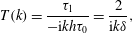 $$\begin{eqnarray}T(k)=\frac{\unicode[STIX]{x1D70F}_{1}}{-\text{i}kh\unicode[STIX]{x1D70F}_{0}}=\frac{2}{\text{i}k\unicode[STIX]{x1D6FF}},\end{eqnarray}$$
which curiously is identical, despite the fact that the motivation is different, to the leading term of the laminar result (3.28). Higher-order corrections to (7.1) in the context of an eddy-viscosity model were studied by Luchini & Charru (Reference Luchini and Charru2010).
7.1 The logarithmic layer
Just like the unbounded laminar Couette flow in § 3.1, a turbulent logarithmic layer unbounded at the top and of constant
 $u_{\unicode[STIX]{x1D70F}}$
(a frequent mathematical idealization for the atmospheric boundary layer) is exceptional among open flows because it can remain exactly parallel. (In practice, an unbounded logarithmic layer will often represent the near-wall region of a larger boundary layer of thickness
 $\unicode[STIX]{x1D6FF}$
, where
 $\unicode[STIX]{x1D6FF}$
itself is not constant. But the near-wall layer will become more and more parallel with increasing
 $\unicode[STIX]{x1D6FF}$
, just as the Couette layer does in the corresponding laminar flow.) Therefore this case has no a priori lower bound on its
 $k$
range of validity. However, there is a fundamental difference: the vorticity of laminar Couette flow is constant and in regime 1 (the
 $k$
range where the disturbance caused by a wall perturbation remains inside the Couette layer of a more general boundary layer) the perturbation is rotational everywhere; the vorticity of the logarithmic layer decreases with
 $z$
, and as will be seen, the disturbance caused by a wall perturbation in a logarithmic layer can become effectively irrotational within the layer itself. Therefore, for a turbulent flow this condition corresponds to regime 3.
In fewer words, whereas a laminar open boundary layer has no actual fully developed regime because having one would imply wavelengths longer than the boundary layer itself, a turbulent open boundary layer is free from this constraint because the typical wavelength scale of the spectrum is not fixed by the thickness of the unperturbed boundary layer but by the thickness where vorticity of the perturbation becomes negligible.
In order to find an asymptotic expression for the transfer function in the
 $k\rightarrow 0$
limit of the logarithmic layer, a quasi-static approach (one that is frequently encountered in practice) is to assume that velocity perturbations are approximately irrotational at a sufficiently large distance, and then assume that the shear stress at the wall remains quasi-statically proportional to the square of the tangential inviscid velocity through a fixed friction coefficient
 $c_{f}$
. From
 $\unicode[STIX]{x1D70F}=c_{f}\unicode[STIX]{x1D70C}U_{ext}^{2}/2$
it follows that
 $\unicode[STIX]{x1D70F}_{1}/\unicode[STIX]{x1D70F}_{0}=2\unicode[STIX]{x1D713}^{\prime }(0)/U_{ext}$
. For irrotational flow, from (3.6) and the inviscid boundary condition (3.7) we obtain
 $\unicode[STIX]{x1D713}^{\prime }(0)=|k|hU_{ext}$
, and thus
 $$\begin{eqnarray}T(k)=\frac{\unicode[STIX]{x1D70F}_{1}}{-\text{i}kh\unicode[STIX]{x1D70F}_{0}}=2\text{i}\,\text{sign}(k)\end{eqnarray}$$
(which differs by a factor of 2, this time, from the corresponding laminar formula (3.29)).
This is a general and simple answer, independent of any parameters, and can be very useful in practice. Notice also that
 $U_{ext}$
cancels in the final result and the latter is independent of the Reynolds number, therefore (7.2) can be applied in situations, such as the atmospheric boundary layer, where
 $U_{ext}$
is unspecified or unknown. Nevertheless the above derivation involves an external region; we need to be cautious since it was observed in § 3.3 that the conceptually similar quasi-static approach leading to (3.29) fails in laminar flow. There is no such thing as an open, fully developed, laminar regime 3 because if there was one it would only occur for perturbation wavelengths longer than the boundary layer itself. However, laminar and turbulent flows are essentially different in this respect because, as will now be shown, in turbulent flow the disturbance stays confined inside the logarithmic layer even in the fully developed regime, and the same result as (7.2) can be derived without any reference to an external region.
In a more accurate description, when the disturbance is described by asymptotically separating a turbulent and an inviscid region, the latter is governed by the Rayleigh equation (3.3) rather than by the irrotational equation (3.5). But if we look at the Rayleigh equation in its compact form
 $$\begin{eqnarray}\unicode[STIX]{x1D713}^{\prime \prime }-(k^{2}+U^{\prime \prime }/U)\unicode[STIX]{x1D713}=0\end{eqnarray}$$
for the example of a logarithmic velocity profile
 $U=\unicode[STIX]{x1D705}^{-1}\log (z/z_{0})$
, we can observe that the term
 $-U^{\prime \prime }/U$
equals
 $z^{-2}/\log (z/z_{0})$
, and becomes negligible with respect to
 $k^{2}$
when
 $$\begin{eqnarray}k^{2}z^{2}\log (z/z_{0})\gg 1.\end{eqnarray}$$
This is a milder condition than
 $|k|z\gg 1$
, and therefore there is a non-empty range of
 $z$
, even in an a priori rotational mean-velocity profile, where the inviscid behaviour of the perturbation streamfunction is at leading order irrotational and given by (3.6). (We note that the second-order Rayleigh equation for
 $\unicode[STIX]{x1D713}$
, as opposed to alternate forms where
 $\unicode[STIX]{x1D713}/U$
or
 $p$
appears as the dependent variable, is the canonical one in which only the second and no first derivative appears. It follows that
 $\unicode[STIX]{x1D713}$
approaches its asymptotic exponential behaviour more closely than these other variables.)
At the same time in the turbulent region, for
 $z\ll |k|^{-1}$
where we expect
 $\unicode[STIX]{x1D713}$
to become independent of
 $k$
, the dimensionally consistent expression for the mean turbulent streamfunction is the universal law of the wall, namely
 $\unicode[STIX]{x1D713}_{dim}/\unicode[STIX]{x1D708}_{dim}=f(z)$
where
 $z=z_{dim}u_{\unicode[STIX]{x1D70F}}/\unicode[STIX]{x1D708}_{dim}$
and
 $f(z)$
is a universal function (an interpolating formula for the derivative of which is provided in Luchini Reference Luchini2018a
). When
 $z_{dim}$
is changed into
 $z_{dim}-h_{dim}$
and
 $\unicode[STIX]{x1D70F}_{dim}$
undergoes a yet unknown increment
 $\unicode[STIX]{x1D70F}_{1}$
,
 $z$
changes into
 $$\begin{eqnarray}\displaystyle (z_{dim}-h_{dim})\sqrt{\unicode[STIX]{x1D70F}_{0}+\unicode[STIX]{x1D70F}_{1}}/\unicode[STIX]{x1D70C}_{dim}\unicode[STIX]{x1D708}_{dim}=(1-h/z)\sqrt{1+\unicode[STIX]{x1D70F}_{1}/\unicode[STIX]{x1D70F}_{0}}\,z\simeq z-h+(\unicode[STIX]{x1D70F}_{1}/2\unicode[STIX]{x1D70F}_{0})z. & & \displaystyle\end{eqnarray}$$
At linear order the streamfunction correction thus becomes
 $\unicode[STIX]{x1D713}(z)=[(\unicode[STIX]{x1D70F}_{1}/2\unicode[STIX]{x1D70F}_{0})z-h]\unicode[STIX]{x1D6F9}^{\prime }(z)=[(\unicode[STIX]{x1D70F}_{1}/2\unicode[STIX]{x1D70F}_{0})z-h]U(z)$
. Since the ranges where
 $|k|z\ll 1$
and (7.4) is valid overlap, this
 $\unicode[STIX]{x1D713}$
must match the low-
 $|k|z$
behaviour of (3.6), i.e. it must be proportional to
 $1-|k|z$
. It follows that
 $$\begin{eqnarray}\unicode[STIX]{x1D70F}_{1}/\unicode[STIX]{x1D70F}_{0}=2|k|h,\end{eqnarray}$$
from which (7.2) ensues again. It is thus no longer surprising that at the end of the previous, more handwaving derivation,
 $U_{ext}$
disappeared in the final result.
More generally we can state that
 $U(|k|^{-1})$
plays in a turbulent flow much of the same role that
 $U_{ext}$
played in a laminar flow, because vorticity of the base flow becomes negligible for
 $z\gg |k|^{-1}$
. In the same range (7.4) where
 $\unicode[STIX]{x1D713}$
is well approximated by (3.6), pressure is nevertheless determined by the full Rayleigh equation (3.3b
), i.e.
 $$\begin{eqnarray}p=-U\unicode[STIX]{x1D713}^{\prime }+U^{\prime }\unicode[STIX]{x1D713}.\end{eqnarray}$$
Since
 $-\unicode[STIX]{x1D713}/\unicode[STIX]{x1D713}^{\prime }=|k|^{-1}\ll U/U^{\prime }=z\log (z/z_{0})$
, this expression can be seen as the Taylor expansion of
 $U(z)$
by the increment
 $|k|^{-1}$
, namely
 $$\begin{eqnarray}p(z)\simeq |k|U(z+|k|^{-1})\unicode[STIX]{x1D713}(z).\end{eqnarray}$$
But we know that
 $p$
must become approximately constant for
 $|k|z\ll 1$
, therefore the value of this constant is
 $p(0)=|k|U(|k|^{-1})\unicode[STIX]{x1D713}(0)$
, and the admittance of the inviscid flow is
 $$\begin{eqnarray}Y_{ext}\simeq \text{i}[U(|k|^{-1})]^{-1}\,\text{sign}(k).\end{eqnarray}$$
As compared to the expression (3.21) for the admittance in laminar flow, in (7.9)
 $U_{ext}=U(\infty )$
has been replaced by
 $U(|k|^{-1})$
, which becomes
 $U_{ext}$
again if by accident
 $|k|^{-1}>\unicode[STIX]{x1D6FF}$
. This result only indirectly depends on whether the flow is laminar or turbulent, through the boundary-layer thickness
 $\unicode[STIX]{x1D6FF}$
being smaller or larger than the wavelength. Whereas a laminar boundary layer can easily be thinner that the wavelength, and when it is not it falls in the zero-admittance regime 1 (or 0) which is independent of the boundary-layer thickness anyway, a turbulent boundary layer is nearly always thicker than, or of thickness at least comparable to, the wavelength; as a consequence much of its behaviour becomes independent of the actual thickness (and therefore of the Reynolds number). In sharp contrast to open laminar flow, the transfer function of open turbulent flow resulting from the expression (7.9) for the admittance will only contain the velocity
 $U(|k|^{-1})$
and never
 $U_{ext}$
.
7.2 Quasi-laminar response
After regime 0 ends, when
 $k$
progressively decreases below
 $1$
, perturbations will progressively extend over a turbulent and an inviscid region, the turbulent region being the analogue of the viscous region that existed in the laminar case. For
 $k$
smaller than unity but still not too small, the perturbation diffusion layer remains inside the viscous sublayer of the turbulent stream and we can then treat this diffusion layer as laminar, taking into account molecular viscosity only, whereas the inviscid layer will be affected by the mean value of the turbulent velocity. It was empirically shown in Luchini & Charru (Reference Luchini and Charru2017) that this is the case when
 $k\gtrsim 10^{-2}$
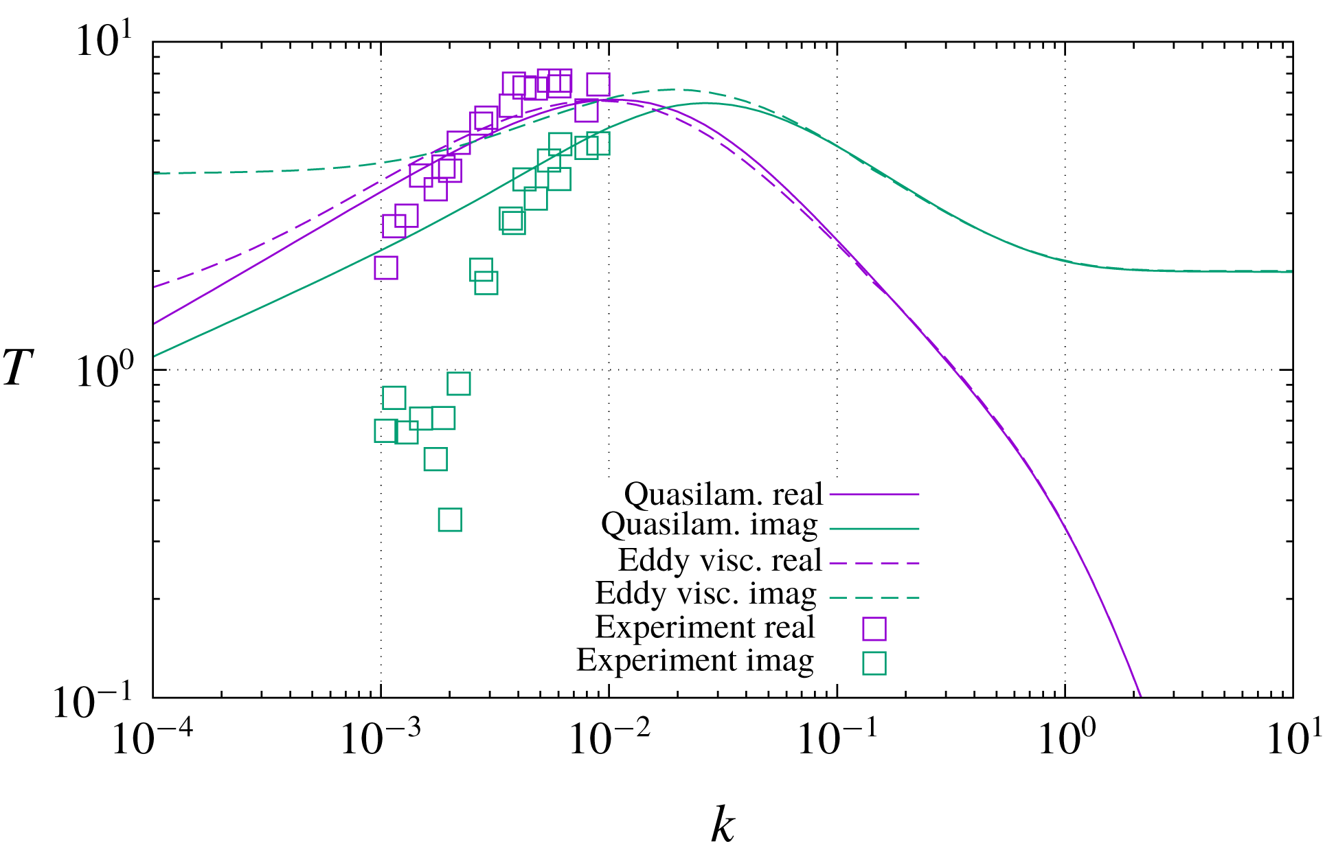
. There, we denoted this region of the spectrum as ‘quasi-laminar’, using the same terminology originally introduced by Thorsness et al. (Reference Thorsness, Morrisroe and Hanratty1978), implying that the resulting transfer function combines laminar viscosity with the shape of the turbulent mean-velocity profile. In practice, it ensues from the coupling of a viscous boundary layer, where only molecular viscosity operates, and an inviscid region in which viscous and turbulent diffusion are both negligible as far as the perturbation is concerned, but the mean-velocity profile is that of the turbulent base flow. This quasi-laminar perturbation regime can then be numerically described by the Orr–Sommerfeld equation containing the actual mean turbulent flow but with molecular viscosity only. We must emphasize, however, that in Luchini & Charru (Reference Luchini and Charru2017) we used the classical Orr–Sommerfeld equation (2.1) for this purpose. It had already been observed by Thorsness et al. (Reference Thorsness, Morrisroe and Hanratty1978) that when Hanratty’s equation (5.2) is substituted for Benjamin’s the approximation improves (see figure 5 of Thorsness et al.
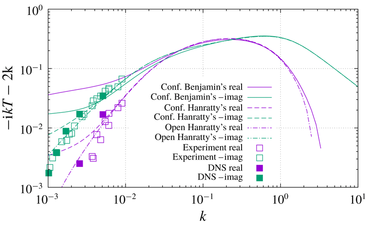
Reference Thorsness, Morrisroe and Hanratty1978). When the numerical computation is repeated using Hanratty’s equation (5.7), the result of Luchini & Charru (Reference Luchini and Charru2017) becomes the one shown in figure 6 for confined and in figure 7 for open flow.


In order to ease the comparison, figure 6 has been drawn with the same axes as figure 2 of Luchini & Charru (Reference Luchini and Charru2017). In particular,
 $T$
as defined in Luchini & Charru (Reference Luchini and Charru2017) equals the present
 $-\text{i}kT$
, the ratio between wall shear stress and the Fourier transform of the height
 $h$
rather than of slope
 $h_{x}$
. The curves tagged ‘confined Benjamin’s’ reproduce the same data as in Luchini & Charru (Reference Luchini and Charru2017), the solution of the classical Orr–Sommerfeld equation (2.1) for confined flow in a symmetrical channel at
 $\text{Re}_{\unicode[STIX]{x1D70F}}=400$
. The ‘confined Hanratty’s’ curves represent the solution of (5.7) for an identical confined flow. The ‘open Hanratty’s’ curves represent the solution of (5.7) for an open boundary layer at the same Reynolds number (actually, as will be seen next, the Reynolds number is irrelevant), with the mean flow provided by the accurate interpolation of the turbulent law of the wall recently developed and given in Box 1 of Luchini (Reference Luchini2018a
). Clearly the adoption of Hanratty’s equation (5.7) in place of Benjamin’s (2.1) considerably extends to the left the range of
 $k$
where agreement is observed with both the experimental measurements of Abrams & Hanratty (Reference Abrams and Hanratty1985) and the direct numerical simulations of Luchini (Reference Luchini2016, Reference Luchini2017), especially so as far as the real part is concerned. Agreement becomes even better with the quasi-laminar calculation in the open regime, for reasons that will be analysed below, and shows that the quasi-laminar regime extends over the whole range
 $k\gtrsim 10^{-3}$
.

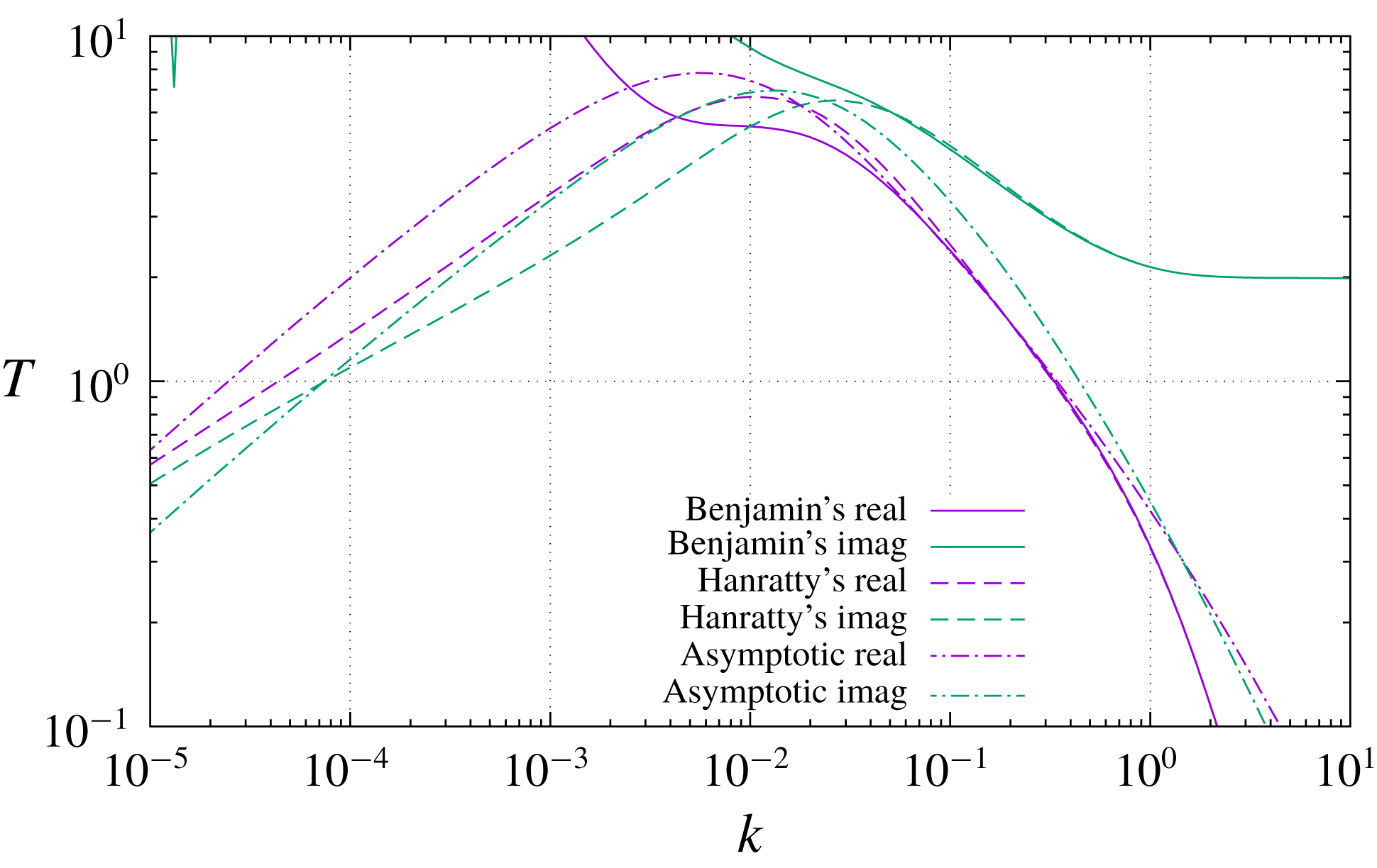
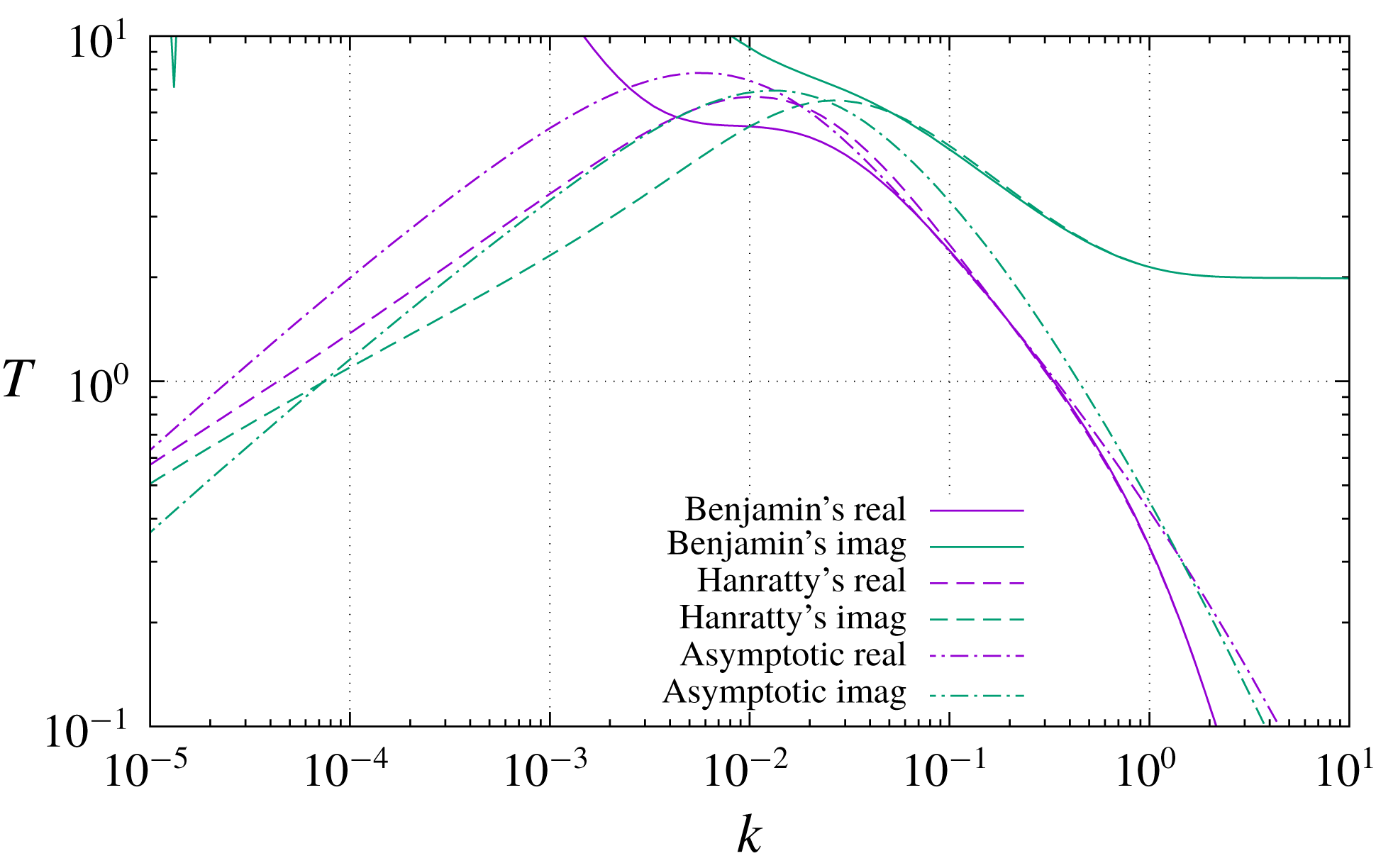
The comparison between calculations of the shear-stress transfer function of open flow according to Benjamin’s and Hanratty’s formulations appears in figure 7, with the mean flow given by the analytical approximation of the law of the wall of Luchini (Reference Luchini2018a
), for
 $\text{Re}_{\unicode[STIX]{x1D70F}}=400$
. Just as was the case for laminar flow in the corresponding figure 4, here the differences are much more marked than in confined flow, and left of the maximum located at
 $k\approx 10^{-2}$
the curve obtained from Benjamin’s formulation diverges with decreasing
 $k$
while the one obtained from Hanratty’s, correct, formulation decreases. Even without a complete asymptotic analysis, we can propose a very simple approximation obtained, on the basis of the considerations leading to (7.9) above, by just substituting
 $U(|k|^{-1})$
for
 $U_{ext}$
into the laminar asymptotic formula (3.24); this is also plotted in figure 7 and the agreement is reasonable. Both the laminar and turbulent transfer functions have a maximum, which endows them with a kind of resonance at a characteristic wavenumber, but the most striking difference between them is that, whereas the laminar peak-response wavenumber changes like
 $\unicode[STIX]{x1D6FF}^{-3/2}$
with Reynolds number
 $\text{Re}_{\unicode[STIX]{x1D70F}}=\unicode[STIX]{x1D6FF}$
, the turbulent peak-response wavenumber is a fixed value of the order of
 $k\approx 10^{-2}$
for all Reynolds numbers. In other words the quasi-laminar turbulent transfer function (which is a good approximation to the true turbulent transfer function in this region) becomes quickly Reynolds number independent contrary to the laminar one. This independence can be ascribed, as discussed in general at the beginning of § 7, to the turbulent boundary layer being comparatively much thicker, which makes its actual thickness irrelevant. For the same reason, a proper asymptotic theory is impossible, because the position and intensity of the maximum do not change with any parameter; but the approximation obtained by purposely adapting the laminar asymptotic result, the one displayed in the figure, can perhaps be of practical utility.
Reynolds number dependence of the quasi-laminar transfer function.
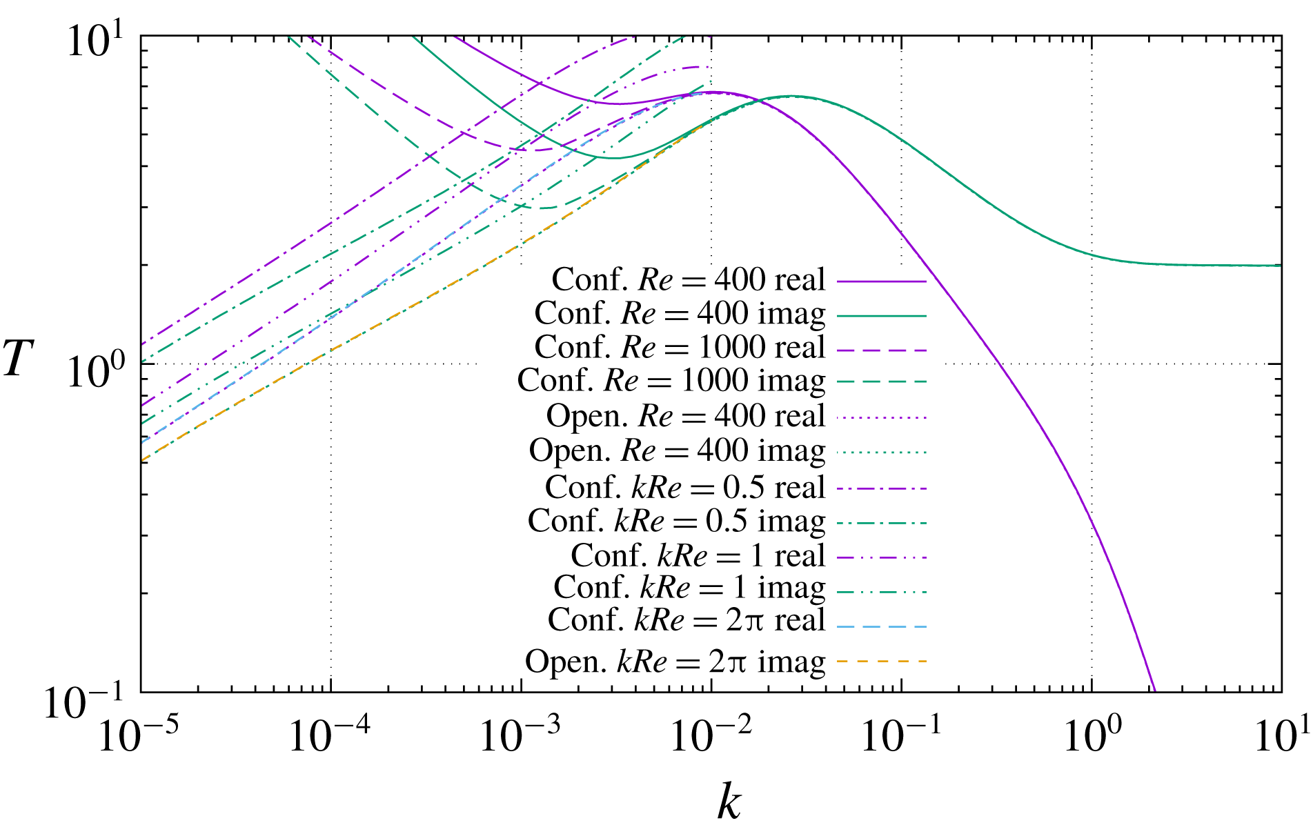
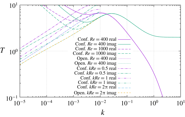
Finally, figure 8 compares the quasi-laminar transfer functions of confined and open flow to each other. All responses displayed coincide for large enough
 $k$
, and then diverge from each other with
 $k$
decreasing. The confined responses diverge from the open response at different positions for different Reynolds numbers (and actually diverge to infinity for
 $k\rightarrow 0$
in compliance with (7.1)), whereas the open responses are perfectly superposed and only one Reynolds number is shown. The curves at constant
 $k\text{Re}$
reproduce conditions, such as in Abrams & Hanratty’s experiment, where a single physical channel having a sinusoidal wall is subjected to a simultaneous change of non-dimensional
 $k$
and Reynolds number by changing the speed of the mean flow. As visible in figure 8, these curves run parallel to the open-flow transfer function. By
 $k\text{Re}=2\unicode[STIX]{x03C0}$
(
 $\unicode[STIX]{x1D706}=\unicode[STIX]{x1D6FF}$
, the actual geometry of Abrams & Hanratty’s channel), the constant-
 $k\text{Re}$
curve is perfectly superposed with the open-flow transfer function, a condition which presumably fulfilled the experimenters’ intention and at the same time explains why the open-flow response provides the best match in figure 6, despite the experiments being performed in a confined channel.
7.3 Eddy viscosity
With some reluctance we include a section about eddy viscosity, because previous work of one of us (Luchini Reference Luchini2016; Russo & Luchini Reference Russo and Luchini2016; Luchini Reference Luchini2018b ) highlighted that, when perturbations to a parallel flow are involved, there is complete disagreement between the predictions of eddy viscosity and direct numerical simulation. Yet, much of the literature about turbulent flow over uneven terrain uses this kind of turbulence modelling (Belcher & Hunt Reference Belcher and Hunt1998); therefore, there is some interest in understanding what modifications of the Orr–Sommerfeld equation are necessary when used in conjunction with an eddy-viscosity model.
7.3.1 Variable viscosity
Some modifications of the problem set-up are needed in general when dealing with a variable viscosity, be it the representation of a turbulent eddy-viscosity model or of an actual inhomogeneous fluid with a viscosity gradient induced by temperature or chemical composition. First, the divergence of the stress tensor cannot be reduced to a Laplacian any more, but the deformation rate must be written in its full symmetric form and derivatives of viscosity must be properly taken into account. This generally complicates the structure of viscous terms, and (2.1) becomes
 $$\begin{eqnarray}-\text{i}k(U\unicode[STIX]{x1D713}^{\prime \prime }-U^{\prime \prime }\unicode[STIX]{x1D713}-k^{2}U\unicode[STIX]{x1D713})=k^{4}\widetilde{\unicode[STIX]{x1D708}}\unicode[STIX]{x1D713}+k^{2}\widetilde{\unicode[STIX]{x1D708}}\unicode[STIX]{x1D713}^{\prime \prime }+k^{2}(\widetilde{\unicode[STIX]{x1D708}}\unicode[STIX]{x1D713})^{\prime \prime }-4k^{2}(\widetilde{\unicode[STIX]{x1D708}}\unicode[STIX]{x1D713}^{\prime })^{\prime }+(\widetilde{\unicode[STIX]{x1D708}}\unicode[STIX]{x1D713}^{\prime \prime })^{\prime \prime }.\end{eqnarray}$$
Second, viscosity
 $\widetilde{\unicode[STIX]{x1D708}}$
is a material property, which can be a function of thermodynamic variables like temperature or chemical composition, or just as well of the statistics of turbulent fluctuations, and follows the perturbations of such quantities. On the assumption that the property that
 $\widetilde{\unicode[STIX]{x1D708}}$
depends upon is simply convected with no diffusion (infinite Schmidt number, see also Ern et al.
Reference Ern, Charru and Luchini2003),
 $\widetilde{\unicode[STIX]{x1D708}}$
must be seen as a given function of the perturbed streamfunction
 $\unicode[STIX]{x1D6F9}+\unicode[STIX]{x1D713}$
, and different from the viscosity
 $\unicode[STIX]{x1D708}(z)$
of the unperturbed parallel flow. From the Taylor expansion
 $\tilde{\unicode[STIX]{x1D708}}(\unicode[STIX]{x1D6F9}+\unicode[STIX]{x1D713})\simeq \unicode[STIX]{x1D708}(z)+(\text{d}\unicode[STIX]{x1D708}/\text{d}z)(\text{d}z/\text{d}\unicode[STIX]{x1D6F9})\unicode[STIX]{x1D713}$
, the product
 $\widetilde{\unicode[STIX]{x1D708}}\unicode[STIX]{x1D713}^{\prime \prime }$
can be linearized as
 $$\begin{eqnarray}\widetilde{\unicode[STIX]{x1D708}}\unicode[STIX]{x1D713}^{\prime \prime }\simeq \unicode[STIX]{x1D708}(z)\unicode[STIX]{x1D6F9}^{\prime \prime }+\unicode[STIX]{x1D708}(z)\unicode[STIX]{x1D713}^{\prime \prime }+\unicode[STIX]{x1D6F9}^{\prime \prime }\frac{\text{d}\unicode[STIX]{x1D708}}{\text{d}z}\frac{\text{d}z}{\text{d}\unicode[STIX]{x1D6F9}}\unicode[STIX]{x1D713},\end{eqnarray}$$
whence, since
 $\unicode[STIX]{x1D6F9}^{\prime }=\text{d}\unicode[STIX]{x1D6F9}/\text{d}z=U$
,
 $$\begin{eqnarray}\displaystyle & & \displaystyle -\text{i}k(U\unicode[STIX]{x1D713}^{\prime \prime }-U^{\prime \prime }\unicode[STIX]{x1D713}-k^{2}U\unicode[STIX]{x1D713})=k^{4}(\unicode[STIX]{x1D708}\unicode[STIX]{x1D713}+\unicode[STIX]{x1D6F9}\unicode[STIX]{x1D708}^{\prime }U^{-1}\unicode[STIX]{x1D713})+k^{2}(\unicode[STIX]{x1D708}\unicode[STIX]{x1D713}^{\prime \prime }+\unicode[STIX]{x1D6F9}^{\prime \prime }\unicode[STIX]{x1D708}^{\prime }U^{-1}\unicode[STIX]{x1D713})\nonumber\\ \displaystyle & & \displaystyle \quad +\,k^{2}(\unicode[STIX]{x1D708}\unicode[STIX]{x1D713}+\unicode[STIX]{x1D6F9}\unicode[STIX]{x1D708}^{\prime }U^{-1}\unicode[STIX]{x1D713})^{\prime \prime }-4k^{2}(\unicode[STIX]{x1D708}\unicode[STIX]{x1D713}^{\prime }+\unicode[STIX]{x1D708}^{\prime }\unicode[STIX]{x1D713})^{\prime }+(\unicode[STIX]{x1D708}\unicode[STIX]{x1D713}^{\prime \prime }+U^{\prime }\unicode[STIX]{x1D708}^{\prime }U^{-1}\unicode[STIX]{x1D713})^{\prime \prime }.\end{eqnarray}$$
Equation (7.12) is the standard Orr–Sommerfeld equation (2.1) according to Benjamin, as adapted to variable-viscosity fluids. In the boundary-layer approximation, when terms proportional to
 $k^{2}$
and higher are neglected, equation (7.12) reduces to
 $$\begin{eqnarray}-\text{i}k(U\unicode[STIX]{x1D713}^{\prime }-U^{\prime }\unicode[STIX]{x1D713})^{\prime }=(\unicode[STIX]{x1D708}\unicode[STIX]{x1D713}^{\prime \prime }+U^{\prime }\unicode[STIX]{x1D708}^{\prime }U^{-1}\unicode[STIX]{x1D713})^{\prime \prime }.\end{eqnarray}$$
The corresponding Hanratty equation, as described in § 5, can be obtained by adding to the right-hand side of either (7.12) or (7.13) the same right-hand side of (7.13) again, but with
 $hU$
in the place of
 $\unicode[STIX]{x1D713}$
, in such a manner that
 $\unicode[STIX]{x1D713}=-hU$
becomes a particular exact solution. Thus the variable-viscosity version of (5.7) becomes
 $$\begin{eqnarray}\displaystyle & & \displaystyle -\text{i}k(U\unicode[STIX]{x1D713}^{\prime \prime }-U^{\prime \prime }\unicode[STIX]{x1D713}-k^{2}U\unicode[STIX]{x1D713})-k^{4}(\unicode[STIX]{x1D708}\unicode[STIX]{x1D713}+\unicode[STIX]{x1D6F9}\unicode[STIX]{x1D708}^{\prime }U^{-1}\unicode[STIX]{x1D713})-k^{2}(\unicode[STIX]{x1D708}\unicode[STIX]{x1D713}^{\prime \prime }+\unicode[STIX]{x1D6F9}^{\prime \prime }\unicode[STIX]{x1D708}^{\prime }U^{-1}\unicode[STIX]{x1D713})\nonumber\\ \displaystyle & & \displaystyle \quad -\,k^{2}(\unicode[STIX]{x1D708}\unicode[STIX]{x1D713}+\unicode[STIX]{x1D6F9}\unicode[STIX]{x1D708}^{\prime }U^{-1}\unicode[STIX]{x1D713})^{\prime \prime }+4k^{2}(\unicode[STIX]{x1D708}\unicode[STIX]{x1D713}^{\prime }+\unicode[STIX]{x1D708}^{\prime }\unicode[STIX]{x1D713})^{\prime }-(\unicode[STIX]{x1D708}\unicode[STIX]{x1D713}^{\prime \prime }+\unicode[STIX]{x1D6F9}^{\prime \prime }\unicode[STIX]{x1D708}^{\prime }U^{-1}\unicode[STIX]{x1D713})^{\prime \prime }\nonumber\\ \displaystyle & & \displaystyle \quad =h(\unicode[STIX]{x1D708}U^{\prime \prime }+U^{\prime }\unicode[STIX]{x1D708}^{\prime })^{\prime \prime }=h(\unicode[STIX]{x1D708}U^{\prime })^{\prime \prime \prime }.\end{eqnarray}$$
Notice that, if the equilibrium of the parallel base flow is written as
 $$\begin{eqnarray}(\unicode[STIX]{x1D708}U^{\prime })^{\prime }+F=0,\end{eqnarray}$$
with a real or fictitious volume force
 $F$
, the corrective term equals
 $-hF^{\prime \prime }$
, just as was the case for constant viscosity.
7.3.2 Turbulent flow as a variable-viscosity fluid
When a turbulent flow is modelled through an eddy viscosity, this variable viscosity can be considered to be a known function of coordinates (zero-equation model), or of auxiliary properties such as turbulent energy, dissipation or Reynolds stresses (one, two or more equation models). In parallel flow, all these models become equivalent to each other, because the auxiliary properties are functions of
 $z$
only and so is viscosity, but the equivalence in principle disappears when an
 $x$
-dependence is reintroduced. The most cited asymptotic eddy-viscosity analysis of flow over a perturbed bottom (Jackson & Hunt Reference Jackson and Hunt1975) is based on a zero-equation model and to this choice we shall adhere here. Nevertheless, in the presence of a perturbation of the shape of the bottom wall it would be unreasonable to assume that
 $\unicode[STIX]{x1D708}$
remains the same function of the distance to the unperturbed wall (nor do Jackson & Hunt Reference Jackson and Hunt1975, assume it); therefore we shall treat the turbulent flow as a variable-viscosity fluid where viscosity remains attached to streamlines, as in the previous section.
As an additional simplification, since according to § 7.2 turbulence only affects the transfer function for
 $k\ll 1$
, we shall neglect terms proportional to
 $k^{2}$
and
 $k^{4}$
in the viscous part of (7.14), which thus becomes
 $$\begin{eqnarray}-\text{i}k(U\unicode[STIX]{x1D713}^{\prime \prime }-U^{\prime \prime }\unicode[STIX]{x1D713}-k^{2}U\unicode[STIX]{x1D713})-(\unicode[STIX]{x1D708}\unicode[STIX]{x1D713}^{\prime \prime }+U^{\prime }\unicode[STIX]{x1D708}^{\prime }U^{-1}\unicode[STIX]{x1D713})^{\prime \prime }=h(\unicode[STIX]{x1D708}U^{\prime })^{\prime \prime \prime }.\end{eqnarray}$$
We have numerically verified that adding back the terms in
 $k^{2}$
and
 $k^{4}$
does not visibly change the results that are presented in what follows, except in the
 $k\gtrsim 1$
range where turbulence is irrelevant anyway.
As far as the expression of
 $\unicode[STIX]{x1D708}(z)$
is concerned, a classical choice (and the one adopted in Luchini & Charru Reference Luchini and Charru2010) is to obtain
 $\unicode[STIX]{x1D708}(z)$
from the mean flow (or vice versa) in such a manner that
 $\unicode[STIX]{x1D708}(z)U^{\prime }(z)=\text{const}$
. For the present non-dimensionalization in wall units, the constant is 1 and this choice corresponds to
 $$\begin{eqnarray}\unicode[STIX]{x1D708}(z)=[U^{\prime }(z)]^{-1}.\end{eqnarray}$$
An equally popular, but not practically different, choice is a mixing-length model, where the primitive quantity is a mixing length
 $l_{dim}(z)$
such that
 $$\begin{eqnarray}\unicode[STIX]{x1D70F}_{dim}/\unicode[STIX]{x1D70C}=\unicode[STIX]{x1D708}_{dim}U_{dim}^{\prime }+[l_{dim}U_{dim}^{\prime }]^{2}.\end{eqnarray}$$
Near the wall, the mixing length must be a non-dimensional function when expressed in wall units, i.e.
 $l_{dim}=(\unicode[STIX]{x1D708}_{dim}/u_{\unicode[STIX]{x1D70F}})l(z)$
. With this substitution, and
 $u_{\unicode[STIX]{x1D70F}}$
defined from the local shear stress according to
 $u_{\unicode[STIX]{x1D70F}}^{2}=\unicode[STIX]{x1D70F}_{dim}/\unicode[STIX]{x1D70C}$
, (7.18) becomes
 $$\begin{eqnarray}1=\frac{U^{\prime }}{\unicode[STIX]{x1D70F}}+l^{2}\frac{{U^{\prime }}^{2}}{\unicode[STIX]{x1D70F}^{2}},\end{eqnarray}$$
which implicitly defines
 $\unicode[STIX]{x1D708}(z)=\unicode[STIX]{x1D70F}/U^{\prime }$
as a unique function of
 $l(z)$
. The eddy-viscosity and mixing-length models are therefore totally interchangeable and (7.17) remains valid. As a remark, with the choice (7.17) of the eddy viscosity, the r.h.s. of (7.16) vanishes just as it did in a laminar Couette layer. Infinite-Schmidt-number convection of the viscosity is sufficient to ensure the Prandtl invariance of the Orr–Sommerfeld equation in this particular example.
Eddy-viscosity transfer function for open turbulent flow, according to Benjamin’s and Hanratty’s equations for variable-viscosity fluids.
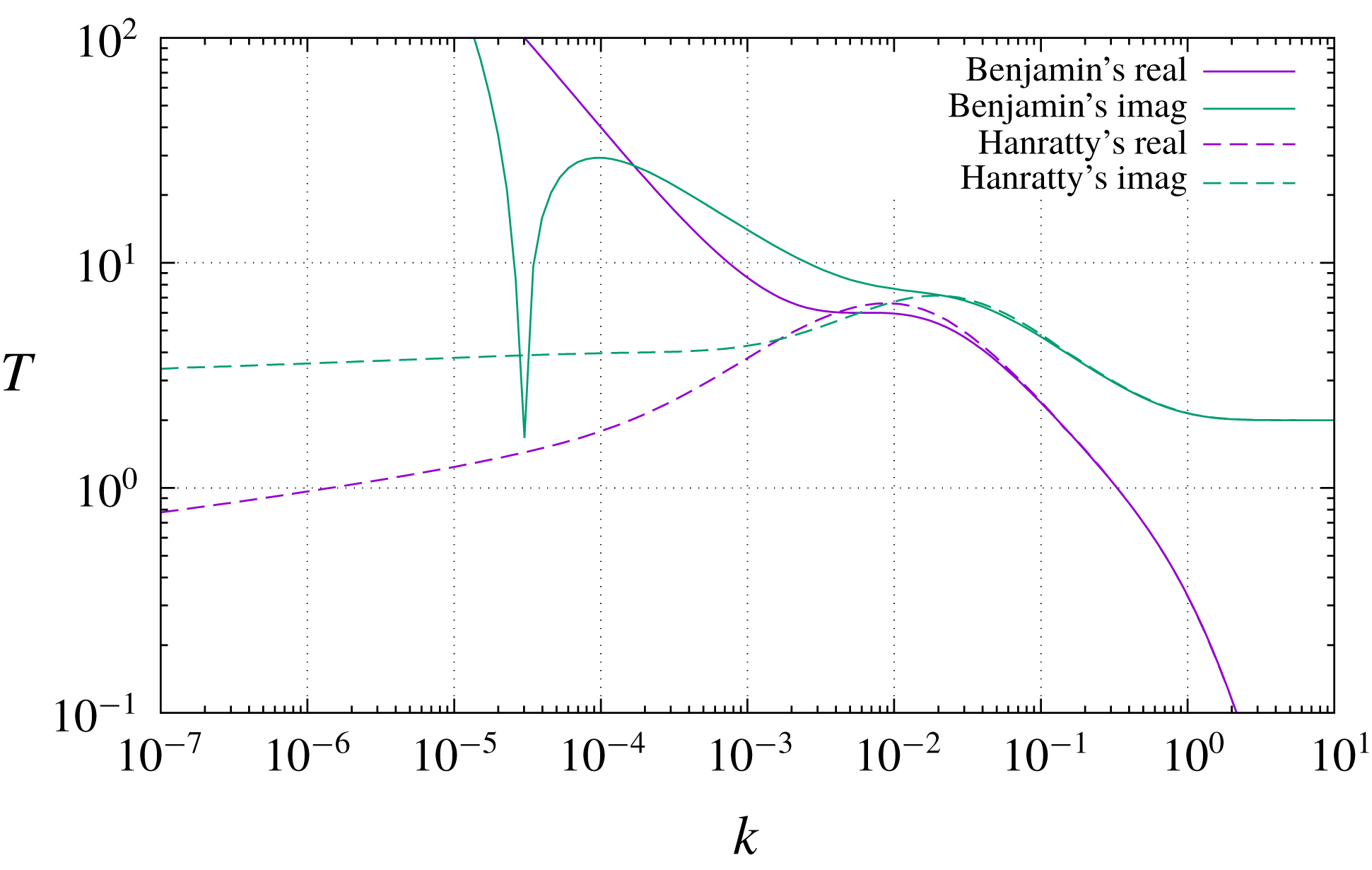
Figure 9 displays the shear-stress transfer function obtained from Benjamin’s and Hanratty’s equations for the eddy-viscosity model (7.17), as applied to open flow with a velocity profile given by the law of the wall of Luchini (Reference Luchini2018a
). Just like in previous examples, the solution of the classical Orr–Sommerfeld equation diverges left of
 $k\approx 10^{-2}$
and fails to represent reasonable behaviour. The solution of Hanratty’s equation, on the other hand, exhibits a maximum in both its real and imaginary parts at about this value, and very slowly decreases towards a constant limit for
 $k\rightarrow 0$
, expected to be the fully developed limit (7.2) even if not realized for any practical
 $k$
. It should be noted that this is very similar to the curve exhibited in figure 3 of Charru et al. (Reference Charru, Andreotti and Claudin2013), also obtained from an eddy-viscosity model.
Comparison of the eddy-viscosity and quasi-laminar open-flow transfer functions with the experiments of Abrams & Hanratty (Reference Abrams and Hanratty1985) for
 $k\unicode[STIX]{x1D6FF}=2\unicode[STIX]{x03C0}$
.
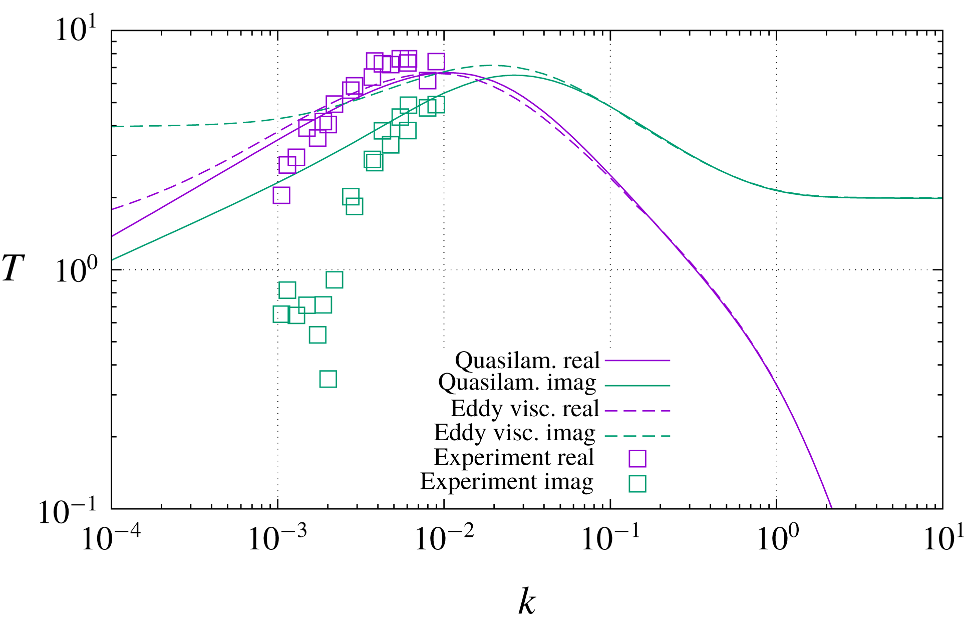
The comparison between the quasi-laminar and eddy-viscosity results is carried forward in figure 10, which also superposes the experimental transfer function of Abrams & Hanratty (Reference Abrams and Hanratty1985). Here we observe that the eddy-viscosity solution nowhere improves upon the quasi-laminar result, and actually completely fails to capture the dip in amplitude that the experimental results (and the direct numerical simulations of Luchini Reference Luchini2016, Reference Luchini2017) exhibit somewhere in the
 $k\approx 10^{-3}$
region. This dip was a subject of major attention by Hanratty’s group, and was successfully reproduced by empirically introducing a first-order spatial delay in the expression of the mixing length. However, like all previous and subsequent authors, they implicitly took it for granted that the transfer function would eventually attain a quasi-static eddy-viscosity behaviour for small enough
 $k$
. Their experiments did not extend to such low
 $k$
as to actually observe this behaviour, and that an eddy viscosity is even valid in the
 $k\rightarrow 0$
limit was recently disproved by a confined-flow numerical counterexample in Russo & Luchini (Reference Russo and Luchini2016). What physically happens in open turbulent flow over a perturbed wall for wavenumbers below
 $10^{-3}$
(wavelengths larger than
 $\unicode[STIX]{x1D706}\approx 6000$
) remains open to speculation.
8 Summary and conclusion
8.1 Laminar flow
The theory of linearized flow over a perturbed terrain classically (Benjamin Reference Benjamin1959) leads to the Orr–Sommerfeld equation as its mathematical description (in its unstationary or stationary version according as the boundary moves or is steady). However, we have seen that, at least in some regimes, the numerical solution of the Orr–Sommerfeld equation fails to provide consistent results and a correction is needed. This correction remained invisible for a long time because in the asymptotic approximations, which preceded the use of computers, it appears natural to treat boundary layers like boundary layers, without recognizing that doing so falls out of the domain of the Orr–Sommerfeld approximation. On the other hand, the numerical solution of the same equation, as close to exact as desired, fails to provide the expected results. With hindsight one can recognize that the asymptotic approximations had used more information than strictly contained in the Orr–Sommerfeld equation.
To understand the origin of this dichotomy one needs to distinguish between confined and open flows, and to partition the wavenumber spectrum in several ranges, or regimes, as we did in table 1 for laminar flow. The perturbation induced by the boundary deformation extends normally into the flow according to two characteristic length scales, a viscous scale
 $O(k^{-1/3})$
and an inviscid scale
 $O(k^{-1})$
, and a priori different regimes are expected depending on how each of these scales compares to the thickness
 $\unicode[STIX]{x1D6FF}$
of either the confined channel or the open boundary layer. Curiously, however, owing to the prevalence of other phenomena, nothing special happens when the inviscid length
 $k^{-1}$
crosses
 $\unicode[STIX]{x1D6FF}$
.
In the simpler case of confined flow there are effectively just three regimes: For
 $k\gg 1$
(in viscous units, which implies that the wavelength-based Reynolds number is small) the perturbation simplifies to Stokes flow irrespective of the Reynolds number of the main stream. For
 $k\ll \unicode[STIX]{x1D6FF}^{-3}$
we have a locally one-dimensional perturbation to a fully developed flow, what is often denoted as a ‘long-wave’ approximation; what needs to be emphasized here is that this long-wave regime does not occur for
 $k\ll \unicode[STIX]{x1D6FF}^{-1}$
, as one may be led to believe if
 $\unicode[STIX]{x1D706}$
is considered as the only scale of length, but only under the much stricter condition
 $k\ll \unicode[STIX]{x1D6FF}^{-3}$
where the viscous length touches the opposing wall. In the whole intermediate region,
 $\unicode[STIX]{x1D6FF}^{-3}\ll k\ll 1$
, the asymptotic solution of Charru & Hinch (Reference Charru and Hinch2000) applies, essentially reducible to a perturbed Couette boundary layer. In addition, there is no discrepancy with the numerical solution of the Orr–Sommerfeld equation for confined flow.
When the flow is open, essentially when it is a boundary layer whose thickness
 $\unicode[STIX]{x1D6FF}$
is smaller than the distance to any surrounding solid walls, and a similar condition is obeyed by
 $\unicode[STIX]{x1D706}$
, the special regime 2 appears in addition to other parts of the spectrum that look similar to confined flow. Perturbations in regime 2 can be described as having their own boundary layer and potential flow, tied to each other in a classical hierarchical inner–outer coupling. At leading order the displacement of the wall produces an equal displacement of the whole main boundary layer. According to the translation invariance of Prandtl’s equations, this displacement can happen without any variation in the velocity profile and without any additional stress or pressure on the wall. In the outer region, the displacement produces a potential flow which excites a pressure. This pressure then produces a second-order perturbation to the boundary layer, which is where a stress on the wall finally appears. This wall shear stress is much smaller than the one that would exist at the same
 $k$
under confinement, and turns out to be proportional to
 $U_{ext}^{2}k^{2/3}$
rather than to
 $k^{-2/3}$
. The boundary between the two regimes is found to occur for
 $k\approx \unicode[STIX]{x1D6FF}^{-3/2}$
, which is the point where the admittances of the boundary layer and of the outer flow become comparable, and also the point where the two stress curves cross each other. This is also the wavenumber where the shear-stress response has its maximum, and potentially identifies the most sensitive wavelength for various applications. In a neighbourhood of this maximum, a uniform analytical asymptotic solution was offered (3.24), which is the result of an interactive boundary-layer formulation and encompasses the previous two. Equation (3.24) does not seem to have appeared before in the literature.
The numerical solution of the Orr–Sommerfeld equation essentially confirms the accuracy of the various asymptotic descriptions, but with the exception of regime 2. Here, surprisingly, the Orr–Sommerfeld equation itself is at failure. An essential ingredient of the physical mechanism of regime 2 is the translation invariance of the boundary layer, and the Orr–Sommerfeld equation lacks this property (although in the asymptotic approximation it was just assumed that it had it). In fact, as was shown in § 5, non-parallelism of the boundary layer plays an essential role and invariance is lost when non-parallel terms are removed. Nonetheless, a correction can be devised which restores the required property. This takes the form of a non-homogeneous right-hand side, and can be interpreted in two alternative ways: one requires writing the Orr–Sommerfeld equation first in a curvilinear frame, where its form is complicated by a number of additional terms, and then reverting to the original cartesian frame where only a simple right-hand side remains. The other alternative is to modify the original problem through a (real or artificial) force term which keeps the boundary-layer thickness from growing, and then include in the perturbation equation the perturbation of this force term corresponding to its displacement in solid with the perturbed wall. The two ways lead to the same correction.
From a historical viewpoint it can be remarked that Benjamin (Reference Benjamin1959) in his original formulation made large use of this curvilinear, displaced reference frame, but then concluded that the result was equivalent to the Orr–Sommerfeld equation in the original Cartesian frame without mentioning any correction. Thorsness et al. (Reference Thorsness, Morrisroe and Hanratty1978), on the other hand, used for their (turbulent) numerical computation the curvilinear equation directly, and therefore did not encounter any apparent difficulty.
8.2 Turbulent flow
When the flow is turbulent, the overall picture changes in several respects. To begin with, the scales of the boundary-layer (or channel) thickness and of the main outer velocity no longer coincide in wall units, as they do for laminar flow: the outer velocity is now
 $U_{ext}=O(\log \unicode[STIX]{x1D6FF})$
, where
 $\unicode[STIX]{x1D6FF}$
in wall units coincides with the Reynolds number. But, even more importantly, the maximum of the shear-stress response no longer occurs at a
 $\unicode[STIX]{x1D6FF}$
-dependent position (it was
 $\unicode[STIX]{x1D6FF}^{-3/2}$
for laminar flow), but rather at a fixed value of
 $k$
which (as everywhere else in wall units) is of the order of
 $10^{-2}$
. This can only be considered an empirical ascertainment, as no asymptotic theory makes sense at a fixed value of
 $k$
, but at least qualitatively it follows from the deduction, in § 7.1, that owing to the logarithmic shape of the velocity profile
 $U(|k|^{-1})$
takes on the role that
 $U_{ext}$
used to have in the coupling between boundary layer and outer flow. In fact, boldly substituting
 $U(|k|^{-1})$
for
 $U_{ext}$
in the laminar formula (3.24) gets interestingly close to the numerical result (see figure 7).
Another fortunate circumstance is that the maximum response falls in the quasi-laminar region. The quasi-laminar region of the spectrum is the one where the perturbation only moderately extends beyond the viscous sublayer, to the point that it feels the actual turbulent mean-velocity profile but only the molecular viscosity. In other words, the perturbation is (numerically) calculated from the laminar Orr–Sommerfeld equation in which the turbulent mean velocity appears as the base flow. It was shown in Luchini & Charru (Reference Luchini and Charru2017) that the quasi-laminar transfer function, which is obviously correct at large
 $k$
, where the perturbation is completely inside the viscous sublayer, with decreasing
 $k$
encounters a maximum and then tends to align with the experimental results of Abrams & Hanratty (Reference Abrams and Hanratty1985) and the numerical results of Luchini (Reference Luchini2016, Reference Luchini2017). The novelty here is that, when Hanratty’s equation is inserted in place of the standard one used in Luchini & Charru (Reference Luchini and Charru2017), the agreement with experimental and numerical data improves considerably (see figure 6) and further extends to lower
 $k$
. We can therefore state with some confidence that the quasi-laminar regime extends over most of
 $k>10^{-3}$
, and a region where the shear-stress response is in the range between
 $10^{-2}$
times its maximum and the maximum itself. Once again, the dominant wavelength is likely to fall in this region.
For
 $k<10^{-3}$
, neither experimental nor direct numerical simulation data are, to our knowledge, available. The Orr–Sommerfeld equation can be solved in this region with the aid of an eddy-viscosity turbulence model, and § 7.3 details the modifications that are necessary to do so, in particular the modifications associated with a variable viscosity which can be useful in their own right. Once again, it clearly appears that the modification of Benjamin’s Orr–Sommerfeld equation into Hanratty’s is essential, as without it the response grows unboundedly for
 $k<10^{-2}$
. Despite the modification, however, the eddy-viscosity solution is farther from the numerical and experimental data than the quasi-laminar solution, and does not even appear to capture their trend.
In conclusion, the maximum shear stress of an open turbulent flow in response to wall perturbations occurs, independently of the Reynolds number, for
 $k\approx 10^{-2}$
, and is reasonably well captured by the quasi-laminar analysis. The range
 $k<10^{-3}$
of the spectrum, where anyway the response appears to be much smaller, remains unexplored and offers a challenging but interesting target for future research. The question also remains open whether a fully developed turbulent regime, one where the shear-stress response tends to (7.2), ever exists for open flow at small enough
 $k$
.