1 Introduction
The reflection asymmetry of the solar magnetic activity about the equator is one of the most important properties of the solar dynamo. The magnetic fields of the leading and following sunspot groups of the solar bipolar regions have predominantly opposite polarities in each hemisphere. This is the so-called Hale polarity rule. A similar asymmetry exist for the polar magnetic fields, which are most prominent during the sunspot minima. After Parker (Reference Parker1955), it is commonly accepted that the reflection properties of the large-scale magnetic field are determined by the dynamo mechanism operating inside the Sun. The essential parts of the large-scale dynamo are governed by the differential rotation and the turbulent convective motions. In the convective zone of a star the global rotation makes turbulent convective motions helical. This results in the reflection asymmetry of the convective vortices about the equator and produces the dynamo generation  $\unicode[STIX]{x1D6FC}$-effect, which transforms the global toroidal magnetic field to the poloidal (Parker Reference Parker1955; Krause & Rädler Reference Krause and Rädler1980). The reflection hemispheric asymmetry of the
 $\unicode[STIX]{x1D6FC}$-effect results in the hemispheric asymmetry of the helical properties of the solar magnetic field. This phenomenon is called the hemispheric helicity rule (hereafter HHR) and it is observed in a number of the magnetic helicity tracers like the current helicity in the solar active regions, chirality of the solar prominences etc. The standard HHR suggests a negative sign of the current helicity of solar active regions (ARs) in the northern hemisphere and a positive in the southern one. For the global magnetic field the opposite HHR is expected (Blackman & Brandenburg Reference Blackman and Brandenburg2003). In the ideal situation, there is a hemispheric balance of distributions of the current helicity density and the total magnetic helicity.
The origin of the HHR and its impact on the dynamo is extensively discussed in the literature (see, e.g. the recent review Brandenburg (Reference Brandenburg2018)). Recently Singh et al. (Reference Singh, Käpylä, Brandenburg, Käpylä, Petri, Lagg and Virtanen2018) found that in cycle 24 more than 20 % of the vector magnetic field synoptic maps show violations of the expected hemispheric sign rule. Reversals of the sign rule of the current helicity of solar active regions during the beginning and the end of cycles 22 and 23 have been reported by Zhang et al. (Reference Zhang, Sakurai, Pevtsov, Gao, Xu, Sokoloff and Kuzanyan2010) and references therein. Similar reversals have been found at the end of cycle 24 for the magnetic helicity density by Pipin et al. (Reference Pipin, Pevtsov, Liu and Kosovichev2019). The origin of the HHR reversals was addressed in our previous paper using the mean-field dynamo models (Pipin et al. Reference Pipin, Zhang, Sokoloff, Kuzanyan and Gao2013b). It was found that the reversal of the sign of the small-scale magnetic helicity follows the dynamo wave propagating inside the convection zone and the spatial patterns of the magnetic helicity reversals reflect the processes which contribute to generation and evolution of the large-scale magnetic fields.
In the paper, the HHR will be characterized by the hemispheric sign distribution and the net magnetic helicity parameters, such as the current and magnetic helicity densities. For the perfect HHR the net helicities are about zero and the sign rule is obeyed. The net helicity can be generated by the hemispheric imbalance of the magnetic helicity flux from the surface to the outer atmosphere. The existence of the net helicity flux is still under debate. For example, Georgoulis et al. (Reference Georgoulis, Rust, Pevtsov, Bernasconi and Kuzanyan2009) found that the helicity injection through the solar photosphere associated with active region magnetic fields was well balanced over the solar cycle 23. On the other hand, Yang & Zhang (Reference Yang and Zhang2012) reported significant imbalance between the helicity fluxes of northern and southern hemispheres. Currently, it is unclear to which extent the imbalance of helicity fluxes impacts the dynamo processes inside the convection zone. It is also unclear how the imbalance of helicity fluxes affect the net magnetic helicity density. Another possible reason could be due to redistribution of the magnetic helicity density over the spatial scale. Both effects (helicity fluxes and helicity cascades) are governed by the complicated magnetohydrodynamic processes which can easily destroy the equatorial symmetry from time to time and produce the net magnetic helicity of the Sun.
In the paper we model effects of the net magnetic helicity using the mean-field magneto-hydrodynamic framework. In this case it is important to distinguish magnetic helicity of the small-scale and large-scale (global) fields of the Sun. We represent the magnetic field  $\boldsymbol{B}$ and its vector potential
 $\boldsymbol{A}$ (
 $\boldsymbol{B}=\unicode[STIX]{x1D735}\times \boldsymbol{A}$) as the sum of the mean and fluctuating parts:
 $\boldsymbol{B}=\overline{\boldsymbol{B}}+\boldsymbol{b}$,
 $\boldsymbol{A}=\overline{\boldsymbol{A}}+\boldsymbol{a}$, where the overbar denotes the mean quantities. Next, the magnetic helicity is defined as the integral over the closed domain
 ${\mathcal{H}}=\int \boldsymbol{A}\boldsymbol{\cdot }\boldsymbol{B}\,\text{d}V$, and the
 $\boldsymbol{A}\boldsymbol{\cdot }\boldsymbol{B}$ is the magnetic helicity density. Assuming the validity of the Reynolds rule for averaging of the products and sum of a turbulent quantity, we can distinguish between the contributions of the large-scale and small-scale magnetic fields to the magnetic helicity density
 $$\begin{eqnarray}\overline{\unicode[STIX]{x1D712}}^{(\text{tot})}=\overline{\boldsymbol{A}\boldsymbol{\cdot }\boldsymbol{B}}=\overline{\boldsymbol{A}}\boldsymbol{\cdot }\overline{\boldsymbol{B}}+\overline{\boldsymbol{a}\boldsymbol{\cdot }\boldsymbol{b}}.\end{eqnarray}$$
Hereafter, we denote the small-scale and large-scale parts of the magnetic helicity density as follows,
 $$\begin{eqnarray}\displaystyle & \displaystyle \overline{\unicode[STIX]{x1D712}}=\overline{\boldsymbol{a}\boldsymbol{\cdot }\boldsymbol{b}}, & \displaystyle\end{eqnarray}$$
 $$\begin{eqnarray}\displaystyle & \displaystyle \overline{\unicode[STIX]{x1D712}}^{(m)}=\overline{\boldsymbol{A}}\boldsymbol{\cdot }\overline{\boldsymbol{B}}. & \displaystyle\end{eqnarray}$$
Following Hubbard & Brandenburg (Reference Hubbard and Brandenburg2012), Pipin et al. (Reference Pipin, Sokoloff, Zhang and Kuzanyan2013a), we employ the conservation law for  $\overline{\unicode[STIX]{x1D712}}^{(\text{tot})}$
 $$\begin{eqnarray}\frac{\text{d}}{\text{d}t}\int \overline{\unicode[STIX]{x1D712}}^{(\text{tot})}\,\text{d}V=-2\unicode[STIX]{x1D702}\int \{\overline{\boldsymbol{B}}\boldsymbol{\cdot }\overline{\boldsymbol{J}}+\overline{\boldsymbol{b}\boldsymbol{\cdot }\boldsymbol{j}}\}\,\text{d}V-\int \unicode[STIX]{x1D735}\boldsymbol{\cdot }\boldsymbol{{\mathcal{F}}}^{\unicode[STIX]{x1D712}}\,\text{d}V,\end{eqnarray}$$
where the  $\boldsymbol{{\mathcal{F}}}^{\unicode[STIX]{x1D712}}$ denotes the helicity flux. In the above cited papers it was shown that, with this formulation of the magnetic helicity conservation, the dynamo evolution avoids the catastrophic quenching regimes. The differential equation that corresponds to (1.4) is
 $$\begin{eqnarray}\frac{\unicode[STIX]{x2202}\overline{\unicode[STIX]{x1D712}}^{(\text{tot})}}{\unicode[STIX]{x2202}t}=-\frac{\overline{\unicode[STIX]{x1D712}}}{R_{m}\unicode[STIX]{x1D70F}_{c}}-2\unicode[STIX]{x1D702}\overline{\boldsymbol{B}}\boldsymbol{\cdot }\overline{\boldsymbol{J}}-\unicode[STIX]{x1D735}\boldsymbol{\cdot }\boldsymbol{{\mathcal{F}}}^{\unicode[STIX]{x1D712}}-(\overline{\boldsymbol{U}}\boldsymbol{\cdot }\unicode[STIX]{x1D735})\overline{\unicode[STIX]{x1D712}}^{(\text{tot})}.\end{eqnarray}$$
In the (1.4) we assumed  $2\unicode[STIX]{x1D702}\overline{\boldsymbol{b}\boldsymbol{\cdot }\boldsymbol{j}}=\overline{\unicode[STIX]{x1D712}}/R_{m}\unicode[STIX]{x1D70F}_{c}$ (see, Kleeorin & Rogachevskii Reference Kleeorin and Rogachevskii1999; Kleeorin et al. Reference Kleeorin, Safiullin, Kleeorin, Porshnev, Rogachevskii and Sokoloff2016), where the magnetic Reynolds number
 $R_{m}=10^{3-6}$ and
 $\unicode[STIX]{x1D702}$ is the microscopic diffusivity. Note that conservation law given by (1.4) takes into account the possibility of magnetic helicity fluxes out of the dynamo domain. In the stationary state we have locally
 $$\begin{eqnarray}\overline{\unicode[STIX]{x1D712}}\approx -\overline{\boldsymbol{A}}\boldsymbol{\cdot }\overline{\boldsymbol{B}}=-\overline{\unicode[STIX]{x1D712}}^{(m)}.\end{eqnarray}$$
This balance can be changed in any direction by the helicity fluxes either on the small or the large scales.
We assume that the magnetic helicity density balance is following (1.5) and (1.6). Clearly, there are important unknown details in (1.5), in particular, those are related to the helicity density fluxes. Further, it will be shown that breaking of the equatorial symmetry of the global magnetic field can result in the hemispheric imbalance of the magnetic helicity density, as well. We study the mutual effect of this imbalance and the magnetic parity breaking using mean-field dynamo models.
In § 2 we describe our dynamo model. Section 3 is devoted to description of the main results and to discussion of those results in light of the available observational proxies. Section 4 summarizes our findings.
2 Basic equations
2.1 Dynamo model
In this paper we will discuss the kinematic version of the mean-field dynamo model developed recently by Pipin (Reference Pipin2018) and Pipin & Kosovichev (Reference Pipin and Kosovichev2019). We study the mean-field induction equation in a turbulent perfectly conducting medium
 $$\begin{eqnarray}\frac{\unicode[STIX]{x2202}\overline{\boldsymbol{B}}}{\unicode[STIX]{x2202}t}=\unicode[STIX]{x1D735}\times (\boldsymbol{{\mathcal{E}}}+\overline{\mathbf{U}}\times \overline{\boldsymbol{B}}),\end{eqnarray}$$
where  $\boldsymbol{{\mathcal{E}}}=\overline{\boldsymbol{u}\times \boldsymbol{b}}$ is the mean electromotive force, with
 $\boldsymbol{u},\boldsymbol{b}$ being the fluctuating velocity and magnetic field, respectively,
 $\overline{\mathbf{U}}$ is the mean velocity field, which is represented by the differential rotation and meridional circulation. We assume that the large-scale flow as well as the global thermodynamics of the convection zone remain unaffected by the solar dynamo. Those effects were discussed in the above cited papers. A large-scale axisymmetric magnetic field is represented by decomposition of the sum of the toroidal and poloidal parts
 $$\begin{eqnarray}\overline{\boldsymbol{B}}=\mathbf{e}_{\unicode[STIX]{x1D719}}B+\unicode[STIX]{x1D735}\times \frac{A\mathbf{e}_{\unicode[STIX]{x1D719}}}{r\sin \unicode[STIX]{x1D703}},\end{eqnarray}$$
where  $\unicode[STIX]{x1D703}$ is the polar angle. The mean electromotive force
 $\boldsymbol{{\mathcal{E}}}$ is expressed as follows:
 $$\begin{eqnarray}{\mathcal{E}}_{i}=(\unicode[STIX]{x1D6FC}_{ij}+\unicode[STIX]{x1D6FE}_{ij}^{(\unicode[STIX]{x1D6EC})})\overline{B}_{j}+\unicode[STIX]{x1D702}_{ijk}\unicode[STIX]{x1D735}_{j}\overline{B}_{k}.\end{eqnarray}$$
The tensor  $\unicode[STIX]{x1D6FC}_{ij}$ represents the
 $\unicode[STIX]{x1D6FC}$-effect,
 $\unicode[STIX]{x1D6FE}_{ij}^{(\unicode[STIX]{x1D6EC})}$ is the turbulent pumping and
 $\unicode[STIX]{x1D702}_{ijk}$ is the diffusivity tensor. The
 $\unicode[STIX]{x1D6FC}$ effect includes hydrodynamic and magnetic helicity contributions,
 $$\begin{eqnarray}\displaystyle \unicode[STIX]{x1D6FC}_{ij}=C_{\unicode[STIX]{x1D6FC}}(1+\unicode[STIX]{x1D709}^{(\unicode[STIX]{x1D6FC})}(t,\unicode[STIX]{x1D703}))\unicode[STIX]{x1D6FC}_{ij}^{(H)}+\unicode[STIX]{x1D6FC}_{ij}^{(M)}, & & \displaystyle\end{eqnarray}$$
where  $\unicode[STIX]{x1D709}^{(\unicode[STIX]{x1D6FC})}(t,\unicode[STIX]{x1D703})$ is the fluctuating part of the
 $\unicode[STIX]{x1D6FC}$-effect. Further details about the kinetic part of the
 $\unicode[STIX]{x1D6FC}$ effect,
 $\unicode[STIX]{x1D6FC}_{ij}^{(H)}$, as well as
 $\unicode[STIX]{x1D6FE}_{ij}^{(\unicode[STIX]{x1D6EC})}$,
 $\unicode[STIX]{x1D6FC}_{ij}^{(M)}$ and
 $\unicode[STIX]{x1D702}_{ijk}$ can be found in Pipin & Kosovichev (Reference Pipin and Kosovichev2019). The nonlinear feedback of the large-scale magnetic field to the
 $\unicode[STIX]{x1D6FC}$-effect is described by a dynamical quenching due to the constraint of magnetic helicity conservation given by (1.5). Similar to that paper, the integration domain includes the overshoot layer, which bottom is at
 $r_{b}=0.68R_{\odot }$. The convection zone extends from
 $r_{b}=0.728R_{\odot }$ to
 $r_{e}=0.99R_{\odot }$. We matched the dynamo solution to the potential field outside, and assume zero magnetic field at the bottom boundary. The numerical scheme employs a spatial mesh with 100 nodes in the radius. We use the pseudo-spectral approach for the differentiation operators along latitude and the 64 nodes in latitude are located at the collocation points of the Legendre polynomial. Turbulent coefficients in the bulk of the convection zone are calculated from solution of the mean-field thermodynamic equation using the mixing-length approximation and the mean entropy distribution. It is assumed that in the overshoot layer all the turbulent coefficients except the eddy diffusivity are exponentially quenched. For numerical stability we keep the finite eddy diffusivity in the overshoot layer. More details can be found in Pipin & Kosovichev (Reference Pipin and Kosovichev2019). Distributions of the angular velocity profile, the kinetic part of the
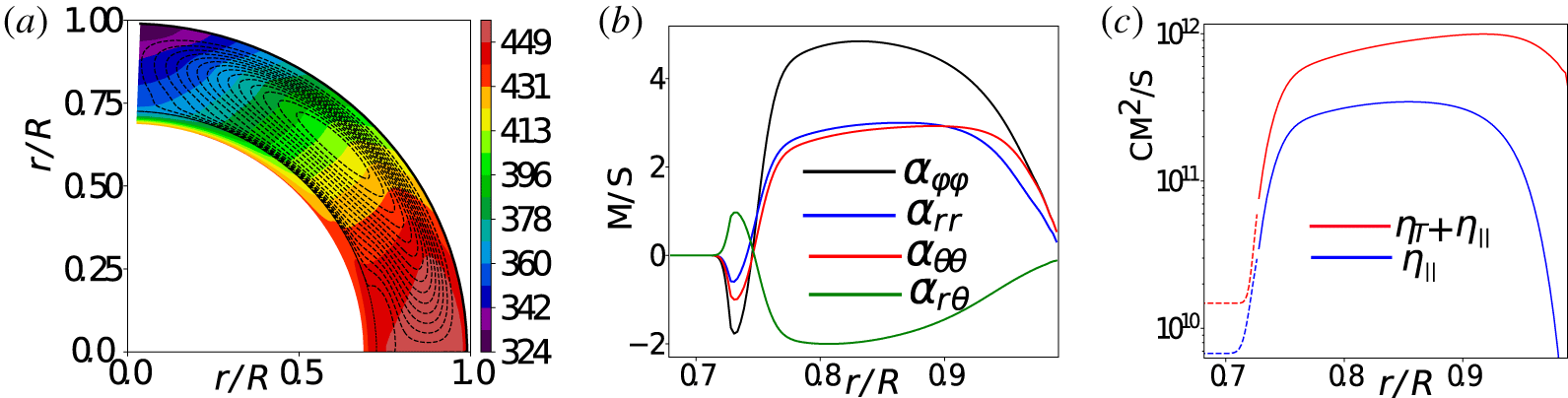
 $\unicode[STIX]{x1D6FC}$ effect tensor and the rotationally anisotropic eddy diffusivity in our model are shown in figure 1. The meridional circulation has the magnitude
 $13~\text{m}~\text{s}^{-1}$ at the surface and it has the stagnation point in the upper part of the convection zone, near
 $0.9R$. The given model describes the dynamo distributed in the bulk of the convection zone. In this model the new dynamo wave starts at the bottom and drifts toward the surface and equator in the main part of the convection zone, below
 $0.9R$. The model of the large-scale flow gives the equatorward meridional circulation in that region. The equatorial drift of the toroidal magnetic field in the subsurface shear layer, i.e. above
 $0.9R$, is provided by the Parker–Yoshimura law (Yoshimura Reference Yoshimura1975) and the latitudinal turbulent pumping; see the detailed discussion of these effects in Pipin (Reference Pipin2018). Similar mechanisms are also suggested by direct numerical simulations, e.g. Warnecke et al. (Reference Warnecke, Käpylä, Käpylä and Brandenburg2016, Reference Warnecke, Rheinhardt, Tuomisto, Käpylä, Käpylä and Brandenburg2018). The given model is one of the numerous variants of the mean-field dynamo models discussed in the literature (Charbonneau Reference Charbonneau2011). The possible choice of the solar dynamo scenario includes the cases with and without the effect of the meridional circulation with the dynamo effects distributed over the convection zone and concentrated in the convection zone boundaries (Choudhuri & Dikpati Reference Choudhuri and Dikpati1999; Brandenburg Reference Brandenburg2005; Cameron & Schüssler Reference Cameron and Schüssler2017). In particular, the models without the meridional circulation (see, e.g. Pipin et al. (Reference Pipin, Zhang, Sokoloff, Kuzanyan and Gao2013b) and their earlier papers) seems to be outdated. Despite the qualitative agreement, the modelled time–latitude evolution of the surface radial magnetic field in is not very consistent with observations. The dynamo model with shallow return flow, such as suggested by Pipin & Kosovichev (Reference Pipin and Kosovichev2019) and considered here, gives qualitatively similar results to our previous models without the meridional circulation. Also, the given model allows us to explain the so-called ‘extended’ mode of the torsional oscillation. The meridional flow can be one of the key factors causing the existence of this mode. This justifies application of the particular variant of the dynamo model for our study.
(a) The reference angular velocity and the streamlines of the meridional circulation distribution; (b) the radial profiles of the  $\unicode[STIX]{x1D6FC}$-effect tensor at latitude
 $45^{\circ }$; (c) radial profiles of the total,
 $\unicode[STIX]{x1D702}_{T}+\unicode[STIX]{x1D702}_{\Vert }$ and the rotationally induced part,
 $\unicode[STIX]{x1D702}_{\Vert }$, of the eddy magnetic diffusivity.

2.2 Random sources of the helicity density imbalance
In our model we explore a few possible sources of the net helicity density. The first is the, non-symmetric about the equator, fluctuations of the kinetic  $\unicode[STIX]{x1D6FC}$-effect (see (2.4)). For deterministic problems like the dynamo equation system, the equations (1.5) and (2.1), which are solved by the standard numerical integration schemes, the spatial and temporal fluctuations of the model parameters are sources of potential numerical pitfalls because the meaning of the derivative is rather different for the deterministic and the random functions. Practically, without going deep into details, we are safe if the typical spatial and temporal scales of the fluctuations are much larger than the size of the spatial mesh and the size of the time step. To simulate the randomness of the
 $\unicode[STIX]{x1D6FC}$-effect distribution over hemispheres we generate spatially random Gaussian sequences,
 $\unicode[STIX]{x1D709}^{(\unicode[STIX]{x1D6FC})}(\unicode[STIX]{x1D703}_{j})$, where
 $\unicode[STIX]{x1D703}_{j}$ are the collocation points of the Legendre polynomials, and
 $\langle \unicode[STIX]{x1D709}^{(\unicode[STIX]{x1D6FC})}(\unicode[STIX]{x1D703}_{j})\rangle =0$,
 $\unicode[STIX]{x1D70E}(\unicode[STIX]{x1D709}^{(\unicode[STIX]{x1D6FC})}(\unicode[STIX]{x1D703}_{j}))=0.5$. Then, we decompose the sequence
 $\unicode[STIX]{x1D709}^{(\unicode[STIX]{x1D6FC})}(\unicode[STIX]{x1D703}_{j})$ in the Legendre polynomials and filter out all the Legendre modes higher than
 $\ell =5$. The resulted latitudinal fluctuations of the
 $\unicode[STIX]{x1D6FC}$-effect are described via the smooth functions. The ensemble of
 $\unicode[STIX]{x1D709}^{(\unicode[STIX]{x1D6FC})}(\unicode[STIX]{x1D703})$ follows the Gaussian probability distribution with a mean approximately equal to 0 and a standard deviation
 $\unicode[STIX]{x1D70E}\approx 0.2$. The renewal time for the sequences
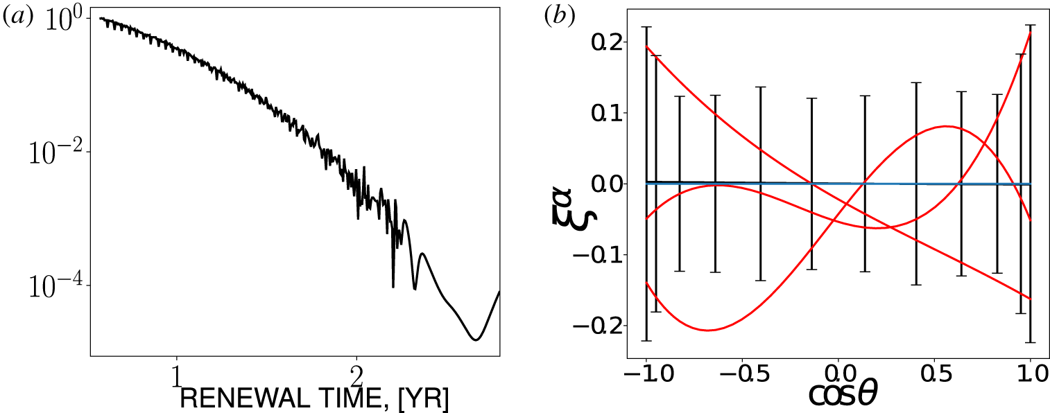
 $\unicode[STIX]{x1D709}^{(\unicode[STIX]{x1D6FC})}$ is also taken in the form of a random sequence. We loosely pick up the values larger than 0.5 year intervals, which is safe for the numerical scheme with a time step of approximately a few hours. The low boundary of the renewal time interval is close to the typical evolution time of the large solar active region (Stenflo Reference Stenflo2013). The probability distribution of the renewal time is shown in figure 2(a). The fluctuations of the
 $\unicode[STIX]{x1D6FC}$-effect in latitude are illustrated in figure 2(b). Note that contribution of
 $\unicode[STIX]{x1D709}^{(\unicode[STIX]{x1D6FC})}(t,\unicode[STIX]{x1D703})$ in (2.4) is multiplied by a factor
 $\cos \unicode[STIX]{x1D703}$ caused by
 $\unicode[STIX]{x1D6FC}_{ij}^{(H)}$.
(a) Probability distribution of the renewal time intervals of  $\unicode[STIX]{x1D709}^{(\unicode[STIX]{x1D6FC})}(t,\unicode[STIX]{x1D703})$; (b) red lines show three realizations of
 $\unicode[STIX]{x1D709}^{(\unicode[STIX]{x1D6FC})}(t,\unicode[STIX]{x1D703})$, the vertical bars show the standard deviations for particular latitudes and the blue line shows the mean over ensemble of realizations,
 $\langle \unicode[STIX]{x1D709}^{(\unicode[STIX]{x1D6FC})}(t,\unicode[STIX]{x1D703})\rangle \approx 0$.

Another source of the net helicity density can be due to the asymmetry about the equator of the flux of helicity density from the dynamo domain to the corona. Following the suggestions by Guerrero, Chatterjee & Brandenburg (Reference Guerrero, Chatterjee and Brandenburg2010) we model this by subtracting the fraction of the helicity density from the local helicity density in the upper parts of the convection zone. Thus, the modified equation for the helicity density evolution is
 $$\begin{eqnarray}\displaystyle \frac{\unicode[STIX]{x2202}\overline{\unicode[STIX]{x1D712}}^{(\text{tot})}}{\unicode[STIX]{x2202}t} & = & \displaystyle -\frac{\overline{\unicode[STIX]{x1D712}}}{R_{m}\unicode[STIX]{x1D70F}_{c}}-2\unicode[STIX]{x1D702}\overline{\boldsymbol{B}}\boldsymbol{\cdot }\overline{\boldsymbol{J}}-\unicode[STIX]{x1D735}\boldsymbol{\cdot }\boldsymbol{F}\nonumber\\ \displaystyle & & \displaystyle -\,\frac{\unicode[STIX]{x1D70F}_{\unicode[STIX]{x1D709}}(r)}{\unicode[STIX]{x1D70F}_{0r}}\sin ^{2}\unicode[STIX]{x1D703}(\unicode[STIX]{x1D709}^{(\unicode[STIX]{x1D712})}(t,\unicode[STIX]{x1D703})\overline{\unicode[STIX]{x1D712}}+\unicode[STIX]{x1D709}^{(m)}(t,\unicode[STIX]{x1D703})\overline{\unicode[STIX]{x1D712}}^{(m)}),\end{eqnarray}$$
where,  $\boldsymbol{F}=-\unicode[STIX]{x1D702}_{\unicode[STIX]{x1D712}}\unicode[STIX]{x1D735}\overline{\unicode[STIX]{x1D712}}$, with
 $\unicode[STIX]{x1D702}_{\unicode[STIX]{x1D712}}=0.1\unicode[STIX]{x1D702}^{(I)}$. Similarly to Pipin et al. (Reference Pipin, Zhang, Sokoloff, Kuzanyan and Gao2013b), we employ
 $R_{m}=10^{6}$. The last term in (2.5) takes into account the helicity density flux out of the solar convection zone. In the paper we study the fluxes of the small-scale and large-scale magnetic helicities. They are
 $\unicode[STIX]{x1D709}^{(\unicode[STIX]{x1D712})}\overline{\unicode[STIX]{x1D712}}$ and
 $\unicode[STIX]{x1D709}^{(m)}\overline{\unicode[STIX]{x1D712}}^{(m)}$, respectively. It is assumed that the fluxes are due to the near surface magnetic activity. Therefore, we apply the factor
 $\sin ^{2}\unicode[STIX]{x1D703}$ and introduce the function
 $$\begin{eqnarray}\unicode[STIX]{x1D70F}_{\unicode[STIX]{x1D709}}(r)={\textstyle \frac{1}{2}}[1-\text{erf}(100(r_{0}-r))],\end{eqnarray}$$
where  $r_{0}=0.9R_{\odot }$ and the dimension factor corresponds to the maximum of the probability density function (PDF) of the renewal time,
 $\unicode[STIX]{x1D70F}_{0r}=0.5~\text{Yr}$ (see figure 2a). In our model we assume that the renewal times for both the large- and small-scale helicity fluxes are the same. This seems counter-intuitive. However, introducing another longer renewal time for the large-scale helicity will introduce a additional free parameter in the model. This is postponed to a future study.
The sequence of the renewal times of the helicity density outflows will be determined in the same way as for the  $\unicode[STIX]{x1D6FC}$-effect except for the low limit, which is approximately ten times smaller and is equal to one month. Thus, the net helicity density flux over a hemisphere is computed as integral over the shell, which includes the subsurface region between
 $r_{0}$ and
 $R_{\odot }$. Functions
 $\unicode[STIX]{x1D709}^{(\unicode[STIX]{x1D712})}$ and
 $\unicode[STIX]{x1D709}^{(m)}$ are random in latitude, and they are defined in the same way as
 $\unicode[STIX]{x1D709}^{(\unicode[STIX]{x1D6FC})}$ and we use the ensembles of the spatial fluctuations with the Gaussian probability function distribution, the mean value of
 $\overline{\unicode[STIX]{x1D709}^{(\unicode[STIX]{x1D712},m)}}=0$ and the standard deviation of
 $\unicode[STIX]{x1D70E}(\unicode[STIX]{x1D709}^{(\unicode[STIX]{x1D712},m)})=1$. These fluctuations are driven with the random renewal time interval, which has the same probability distribution as the
 $\unicode[STIX]{x1D6FC}$ effect fluctuations. For the magnetic helicity density we employ
 $\overline{\unicode[STIX]{x1D712}}=0$ at the bottom and
 $\unicode[STIX]{x1D735}_{r}\overline{\unicode[STIX]{x1D712}}=0$ at the top of the convection zone domain. We neglect the magnetic helicity evolution in the overshoot region for the sake of simplicity.
For the purpose of analysis we introduce the total energy of the dynamo generated magnetic field,
 $$\begin{eqnarray}E_{B}=\frac{1}{8\unicode[STIX]{x03C0}}\int \overline{\boldsymbol{B}}^{2}\,\text{d}V,\end{eqnarray}$$
where integration is over the dynamo domain. Following Pipin, Sokoloff & Usoskin (Reference Pipin, Sokoloff and Usoskin2012), we mimic the sunspot number using parameters of the toroidal magnetic field in the subsurface shear layer
 $$\begin{eqnarray}W=\overline{B}_{\text{max}}(t)\exp \left(-\frac{\overline{B}_{\text{max}}(t)}{B_{0}}\right),\end{eqnarray}$$
where  $B_{0}=600$ G and
 $\overline{B}_{\text{max}}(t)=\max _{\unicode[STIX]{x1D707}=-1:1}((\overline{B}(\unicode[STIX]{x1D707},t)|_{0.95R}))$. In (2.8), we assume that sunspots are produced from the toroidal magnetic fields by means of some nonlinear instability.
The properties of the equatorial symmetry of the magnetic activity is characterized by the parity index. Let us define the parameters characterizing the energy of the symmetric and antisymmetric parts of the radial magnetic field at the surface
 $$\begin{eqnarray}\displaystyle & \displaystyle E_{B}^{S}=\frac{1}{4}\int _{-1}^{1}[\overline{B}_{r}(\unicode[STIX]{x1D707},t)+\overline{B}_{r}(-\unicode[STIX]{x1D707},t)]^{2}\,\text{d}\unicode[STIX]{x1D707}, & \displaystyle\end{eqnarray}$$
 $$\begin{eqnarray}\displaystyle & \displaystyle E_{B}^{N}=\frac{1}{4}\int _{-1}^{1}[\overline{B}_{r}(\unicode[STIX]{x1D707},t)-\overline{B}_{r}(-\unicode[STIX]{x1D707},t)]^{2}\,\text{d}\unicode[STIX]{x1D707}. & \displaystyle\end{eqnarray}$$
Then, the parity index, or the reflection symmetry index for this component of the magnetic activity, is
 $$\begin{eqnarray}P=\frac{E_{B}^{S}-E_{B}^{N}}{E_{B}^{S}+E_{B}^{N}}.\end{eqnarray}$$
Also, we define the parameters characterizing the helicity fluxes of the large- and small-scale magnetic fields. In the model, these fluxes are determined by the random parameters  $\unicode[STIX]{x1D709}^{(\unicode[STIX]{x1D712})}$ and
 $\unicode[STIX]{x1D709}^{(m)}$. For the large-scale magnetic field we define the latitudinal helicity density flux
 $$\begin{eqnarray}F_{L}=-2\unicode[STIX]{x03C0}\sin ^{2}\unicode[STIX]{x1D703}\unicode[STIX]{x1D709}^{(m)}(t,\unicode[STIX]{x1D703})\int _{.9R}^{R}\frac{\unicode[STIX]{x1D70F}_{\unicode[STIX]{x1D709}}(r)}{\unicode[STIX]{x1D70F}_{0r}}\overline{\unicode[STIX]{x1D712}}^{(m)}r^{2}\,\text{d}r.\end{eqnarray}$$
The small-scale magnetic helicity density flux includes the diffusive flux as well, see (2.5),
 $$\begin{eqnarray}\displaystyle F_{S}=-2\unicode[STIX]{x03C0}R^{2}\unicode[STIX]{x1D702}_{\unicode[STIX]{x1D712}}\unicode[STIX]{x1D735}\overline{\unicode[STIX]{x1D712}}|_{.9R}^{R}-2\unicode[STIX]{x03C0}\sin ^{2}\unicode[STIX]{x1D703}\unicode[STIX]{x1D709}^{(\unicode[STIX]{x1D712})}(t,\unicode[STIX]{x1D703})\int _{.9R}^{R}\frac{\unicode[STIX]{x1D70F}_{\unicode[STIX]{x1D709}}(r)}{\unicode[STIX]{x1D70F}_{0r}}\overline{\unicode[STIX]{x1D712}}r^{2}\,\text{d}r. & & \displaystyle\end{eqnarray}$$
Following Berger & Ruzmaikin (Reference Berger and Ruzmaikin2000) and Hawkes & Yeates (Reference Hawkes and Yeates2019) we define the latitudinal helicity density flux due to the differential rotation
 $$\begin{eqnarray}F_{\unicode[STIX]{x1D6FA}}=-4\unicode[STIX]{x03C0}R^{3}\sin \unicode[STIX]{x1D703}\overline{A}\,\overline{B_{r}}\,\overline{U}_{\unicode[STIX]{x1D719}},\end{eqnarray}$$
where  $\overline{A}$ is the vector potential and
 $\overline{U}_{\unicode[STIX]{x1D719}}=R\sin \unicode[STIX]{x1D703}\unicode[STIX]{x1D6FA}(R,\unicode[STIX]{x1D703})$ is the large-scale azimuthal flow at the surface. This helicity flux does not enter directly in the helicity evolution equation. Its effect on the dynamo is determined by the boundary conditions.
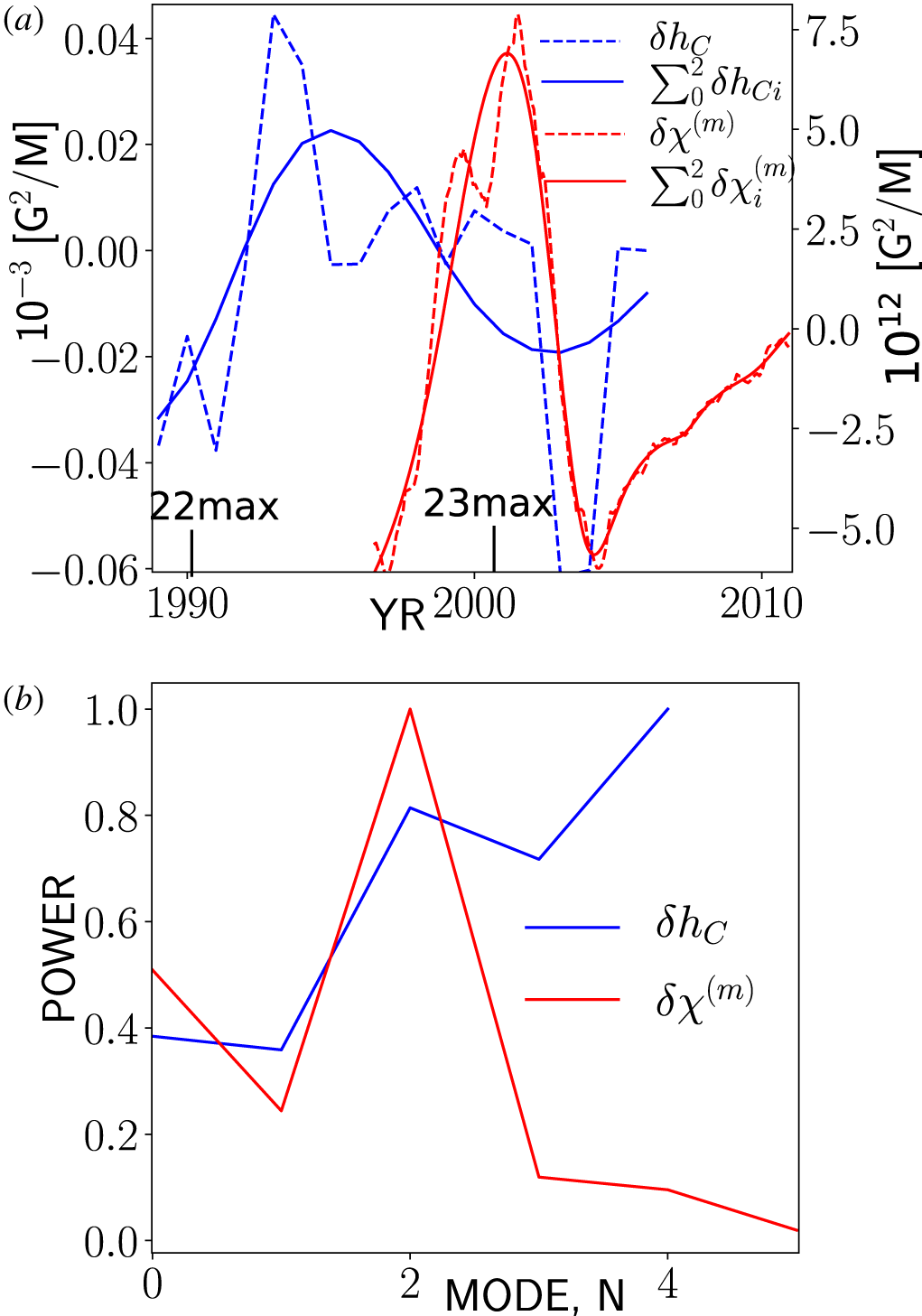
(a) Current helicity density imbalance of the solar ARs (blue colour) and the large-scale magnetic field helicity density imbalance (shown in red colour), and their representation via the first three empirical modes; lines show positions of maxima of the solar cycles 22 and 23; (b) shows the relative power of each mode in the empirical mode decomposition (EMD), where the results are normalized to the maximum of the magnitude of the signal.

3 Observational proxies of the net magnetic helicity
In the Introduction we defined the hemispheric helicity rule by the surface integral of the magnetic helicity proxies. Figure 3(a) shows the integral of the current helicity density of the solar active regions obtained from the reduced data set of the Huairou Solar Observing Station given in Zhang et al. (Reference Zhang, Sakurai, Pevtsov, Gao, Xu, Sokoloff and Kuzanyan2010),
 $$\begin{eqnarray}\unicode[STIX]{x1D6FF}h_{C}=\int _{0}^{1}\overline{h}_{C}\,\text{d}\unicode[STIX]{x1D707},\end{eqnarray}$$
where  $\unicode[STIX]{x1D707}=\cos \unicode[STIX]{x1D703}$ and
 $\unicode[STIX]{x1D703}$ is the polar angle, and the same for the net magnetic helicity density over large and small scales which was reconstructed by Pipin & Pevtsov (Reference Pipin and Pevtsov2014) using the SOHO/MDI data set,
 $$\begin{eqnarray}\unicode[STIX]{x1D6FF}\unicode[STIX]{x1D712}^{(m)}=\int _{0}^{1}\overline{\unicode[STIX]{x1D712}}^{(m)}\,\text{d}\unicode[STIX]{x1D707}.\end{eqnarray}$$
We observe the solar cycle variations of the HHR parameters in both cases. The low cadence of the data set of  $\unicode[STIX]{x1D6FF}h_{C}$ and the limited time interval in both data sets result in uncertainty in our conclusions about the long-term behaviour of these parameters. To get a rough idea we apply the empirical mode decomposition (EMD) method, using the standard PYTHON package, which is available from the SCIPY distribution sets (http://scipy.org). Because of the mentioned issue of our data sets, our analysis is rather rough and it can be subject to systematic aliasing errors. We show the results in the same figure 3(a). The information about the contribution of the empirical modes to the energy of the signal is shown in figure 3(b). In the signal of
 $\unicode[STIX]{x1D6FF}h_{C}$, the ‘small-scale’ modes of short periods, 1–3 years, are the strongest. Their effect on the whole
 $\unicode[STIX]{x1D6FF}h_{C}$ is rather strong over the sunspot minima. The first three modes of
 $\unicode[STIX]{x1D6FF}h_{C}$ show the variation with the solar cycle period. The large-scale magnetic helicity density imbalance has a strong signal with a period of approximately 9 years and the first three modes quite accurately reproduce the total signal. The sum of the first three modes of current helicity density imbalance
 $\sum _{0}^{2}\unicode[STIX]{x1D6FF}h_{C\,i}$ has a similar period. It is seen that
 $\sum _{0}^{2}\unicode[STIX]{x1D6FF}h_{C\,i}$ goes ahead of
 $\sum _{0}^{2}\unicode[STIX]{x1D6FF}\unicode[STIX]{x1D712}_{i}^{(m)}$ with a phase shift of approximately
 $\unicode[STIX]{x03C0}$. This rough analysis shows the possibility of the quasi-regular variations of
 $\unicode[STIX]{x1D6FF}h_{C}$ and
 $\unicode[STIX]{x1D6FF}\unicode[STIX]{x1D712}^{(m)}$ in the dynamo cycle. We shall see whether this effect can be reproduced in our dynamo models.
4 Results
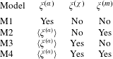
The dynamo model governing parameters are the same as in the paper of Pipin & Kosovichev (Reference Pipin and Kosovichev2019). In all the runs we consider a slightly overcritical dynamo regime using the same dynamo parameter set as in the our previous papers. Similar to those papers, our models are weakly nonlinear with  $\unicode[STIX]{x1D6FD}_{\text{max}}=|B|/\sqrt{4\unicode[STIX]{x03C0}\bar{\unicode[STIX]{x1D70C}}u^{\prime 2}}<0.4$. The random parameters in the models are applied following table 2. Also, table 2 shows some output parameters, like the amplitude of the helicity flux variations, the amplitude of the total magnetic energy and maximum amplitudes of the net helicity in our models.
Random parameters of the model runs. In the models M2, M3 and M4 we neglect the hemispheric asymmetry of the  $\unicode[STIX]{x1D6FC}$-effect fluctuations. In these cases the fluctuating part of the
 $\unicode[STIX]{x1D6FC}$-effect is equal to
 $\langle \unicode[STIX]{x1D709}^{(\unicode[STIX]{x1D6FC})}\rangle (t)$ where we use average over latitudes, see the (2.4).

The integral parameters of the model runs, from left to right: the magnitude of the large-scale helicity flux,  $F_{L}$;
 $F_{S}$ is the same for the small-scale helicity density;
 $F_{\unicode[STIX]{x1D6FA}}$ stands for magnitude of the helicity flux by the differential rotation; the total magnetic energy root mean square (RMS) and its standard deviation (STD); the STD of the net small-scale and large-scale helicity densities,
 $\unicode[STIX]{x1D70E}_{\unicode[STIX]{x1D6FF}\unicode[STIX]{x1D712}}$ and
 $\unicode[STIX]{x1D70E}_{\unicode[STIX]{x1D6FF}\unicode[STIX]{x1D712}m}$, respectively; the last two columns show the RMS and STD of the small-scale and large-scale helicity densities.

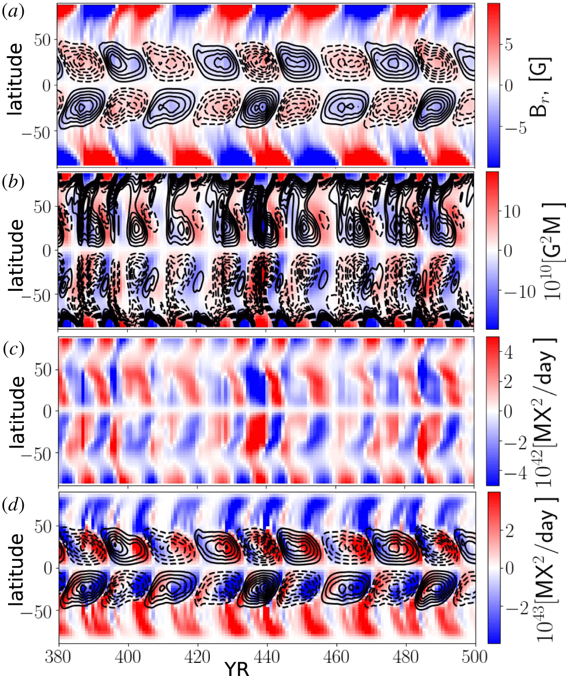
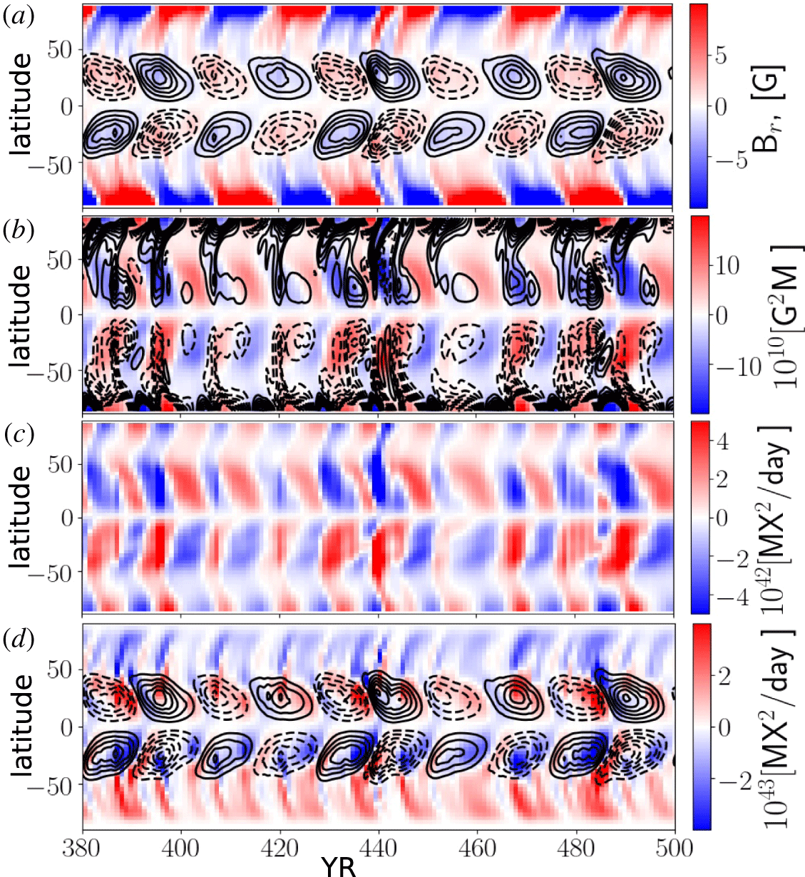
Figures 4 and 5 illustrate the time–latitude diagram of the toroidal magnetic field in the upper part of the solar convection zone, the radial magnetic field at the surface, the time–latitude evolution of the small-scale magnetic helicity density and the fluxes  $F_{L}$,
 $F_{S}$, as well as the flux from the differential rotation,
 $F_{\unicode[STIX]{x1D6FA}}$, see figures 4 and 5(d). The series include episodes of relatively high and weak magnetic activity for the models M2 and M3 (see, also, figure 6). Similar evolution diagrams were found for the models M1 and M4. Evolution patterns of the magnetic field and the HHR for the large- and small-scale magnetic helicity densities are qualitatively similar to our previous results which were discussed in Pipin et al. (Reference Pipin, Zhang, Sokoloff, Kuzanyan and Gao2013b). In particular, for the episodes of high activity, e.g. during years 380–400, our models show the standard HHR for the small- and the large-scale magnetic fields. The inversions of the HHR occur during the relatively short periods of the growing and decaying phases of the magnetic cycles. In the weak cycles these episodes last a longer time. There is a similar tendency in the hemispheric behaviour of the helicity fluxes. The results for the helicity flux due to the differential rotation, i.e.
 $F_{\unicode[STIX]{x1D6FA}}$, are qualitatively similar to the surface flux transport simulations of Hawkes & Yeates (Reference Hawkes and Yeates2019). The amplitude of this flux in our case is an order of magnitude smaller than in theirs because we are restricted to the contribution of the axisymmetric magnetic field. In our simulations the dynamo regimes show that
 $F_{L}<F_{S}<F_{\unicode[STIX]{x1D6FA}}$.
It is found that in the given range variations of the parameters,  $\unicode[STIX]{x1D709}^{(\unicode[STIX]{x1D712})}$,
 $\unicode[STIX]{x1D709}^{(m)},$ the variations of the dynamo efficiency are weak. The magnitude of the maximum total energy of the generated magnetic field among the models varies by approximately 20 % (see table 1). This is likely because the maximum of the dynamo wave is located near the bottom of the convection zone and the dynamo efficiency does not change much because the helicity flux from the surface. On the other hand, it is assumed that random variations of the
 $\unicode[STIX]{x1D6FC}$-effect are uniform in radius. Therefore, the effect of random variations of the
 $\unicode[STIX]{x1D6FC}$-effect is more profound than the effect of the helicity flux variations.
The model M2: (a) the time–latitude diagram of the toroidal magnetic field in the subsurface shear layer (contours in range of  $\pm 600$ G) and the radial magnetic field at the surface (colour image); (b) the time–latitude evolution of the small-scale (colour image) and the large-scale magnetic helicity densities (contours are drawn for the same range of magnitudes
 $\pm 20\times 10^{10}~\text{G}^{2}~\text{M}$); (c) the small-scale magnetic helicity density flux,
 $F_{S}$; (d) the time–latitude diagram of the toroidal magnetic field (same as a) and the magnetic helicity density flux from differential rotation,
 $F_{\unicode[STIX]{x1D6FA}}$ (colour image).

The same as figure 4 for the model M3.

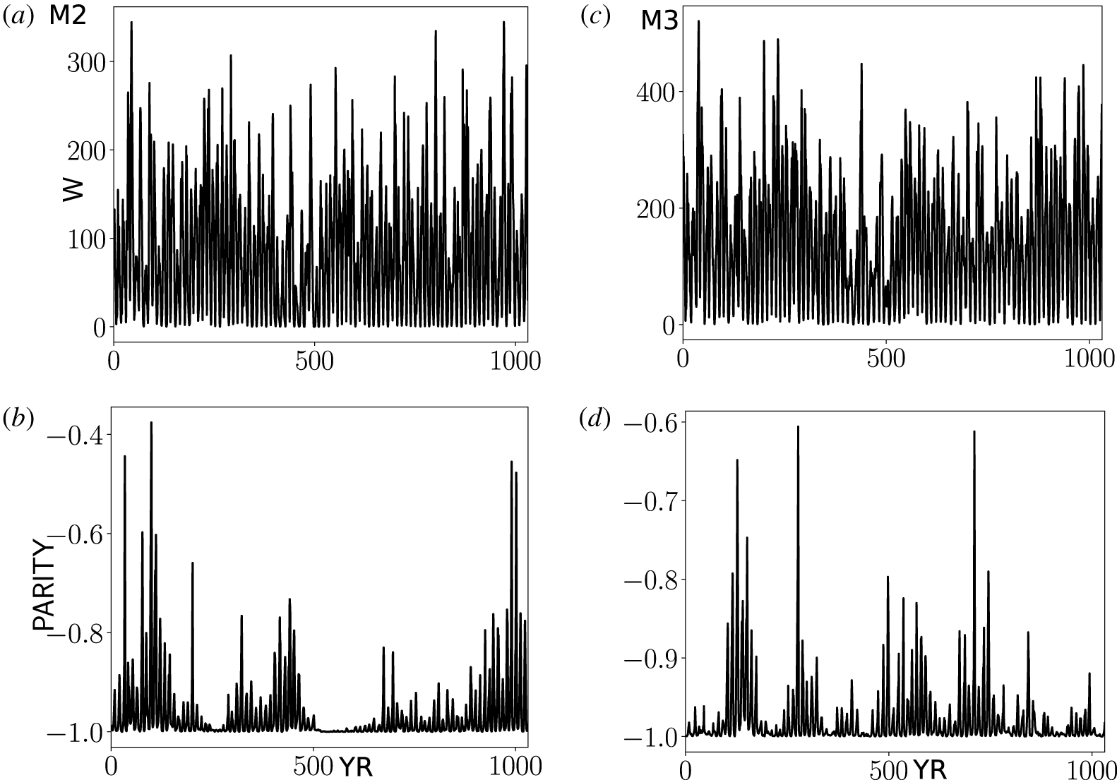
(a) The simulated value of the sunspot number,  $W$ for the model M2; (b) the same for the parity index; (c,d) show the same as (a,b) for the model M3.

Figure 6 shows the simulated value of the sunspot number,  $W$, and the parity index,
 $P$, for the models M2 and M3. The model M3 shows a higher cycle magnitude than the model M2 because the helicity flux from the small-scales increases the dynamo efficiency. The helicity flux from the large-scale magnetic field works in the opposite direction. In contrast, the parity variations are higher in the model M2 than in the model M3.
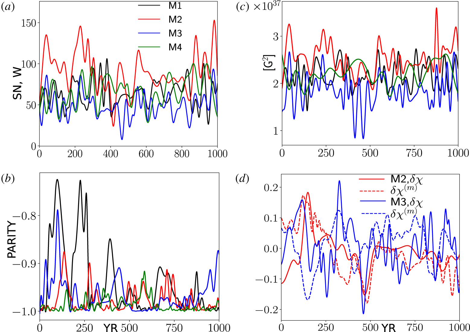
Figure 7 shows the EMD-smoothed series for simulated value of the sunspot number,  $W$, the parity index,
 $P$, and the net magnetic helicity density at the surface for the small-scale and large-scale magnetic fields,
 $\unicode[STIX]{x1D6FF}\unicode[STIX]{x1D712}$ and
 $\unicode[STIX]{x1D6FF}\unicode[STIX]{x1D712}^{(m)}$, respectively, for our models. In this figure we filter out all variations with periods smaller than 20 years using the EMD. The net magnetic helicity densities were normalized to the current RMS helicity densities.
(a) The smoothed simulated value of the sunspot number; (b) the same for the parity index; (c) the same for the total magnetic energy; (d) the same the net magnetic helicity density at the surface.

The results of the model M2 show that, during epochs of the centennial magnetic activity minima, corresponding to periods of around 100, 500 and 900 years, the distributions of the magnetic field and the large-scale magnetic helicity density are not symmetric about the equator and the parity index is greater than  $-1$ during most of the cycle, oscillating around
 $[-0.8:-0.6]$. In contrast, the model M3 shows a tendency for strong deviations of parity during the centennial maximum episodes. This model shows the strongest variations of the sunspot number parameter,
 $W$. Our models show the increase of the parity index seems to be accompanied by and connected with the increase of the oscillation magnitudes of the net helicities
 $\unicode[STIX]{x1D6FF}\unicode[STIX]{x1D712}$ and
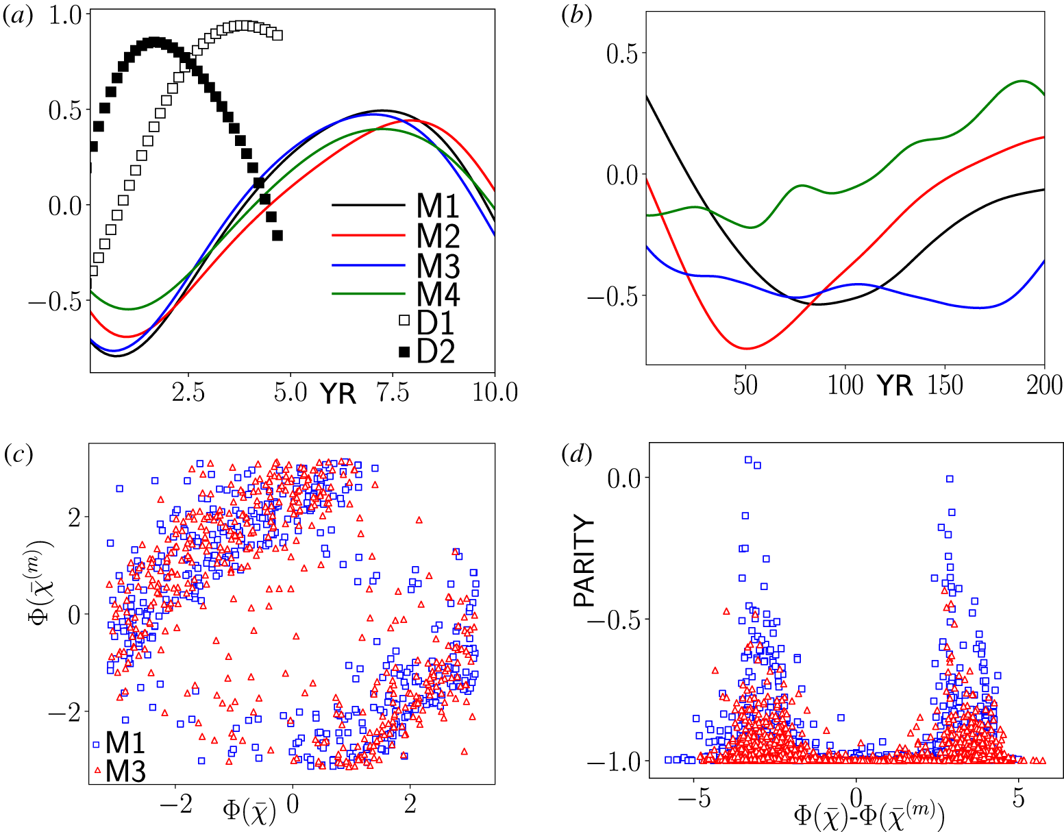
 $\unicode[STIX]{x1D6FF}\unicode[STIX]{x1D712}^{(m)}$. Variations of these parameters on the short time scale, including those within the range of 1 year, go in anti-phase. This effect is quantified by the Pearson correlation coefficient
 $\langle \unicode[STIX]{x1D6FF}\unicode[STIX]{x1D712}(t)\unicode[STIX]{x1D6FF}\unicode[STIX]{x1D712}^{(m)}(t+\unicode[STIX]{x1D70F})\rangle$. It is further illustrated by figure 8(a), where we show results for
 $\langle \unicode[STIX]{x1D6FF}h_{C}(t)\unicode[STIX]{x1D6FF}\unicode[STIX]{x1D712}^{(m)}(t+\unicode[STIX]{x1D70F})\rangle$ computed from our observational data sets and from the models using the original data sets and the smoothed ones where we filter out all variations with periods smaller than 20 years.
(a) The cross-correlations  $\langle \unicode[STIX]{x1D6FF}\unicode[STIX]{x1D712}(t)\unicode[STIX]{x1D6FF}\unicode[STIX]{x1D712}^{(m)}(t+\unicode[STIX]{x1D70F})\rangle$ for the dynamo models and the
 $\langle \unicode[STIX]{x1D6FF}h_{C}(t)\unicode[STIX]{x1D6FF}\unicode[STIX]{x1D712}^{(m)}(t+\unicode[STIX]{x1D70F})\rangle$ from the observational data sets of
 $h_{C}$ and
 $\overline{\unicode[STIX]{x1D712}}^{(m)}$ (D1) and the same correlations computed from the first 3 empirical modes (D2); (b) the same as (a) calculated from the smoothed series of the model runs see figure 7; (c) the phase diagram for phases of the analytical signals of the
 $\unicode[STIX]{x1D6FF}\unicode[STIX]{x1D712}(t)$ and
 $\unicode[STIX]{x1D6FF}\unicode[STIX]{x1D712}^{(m)}(t)$ in the models M1 and M3; (d) the parity index in the models M1 and M3 versus the difference of the phases of the analytical signals of
 $\unicode[STIX]{x1D6FF}\unicode[STIX]{x1D712}(t)$ and
 $\unicode[STIX]{x1D6FF}\unicode[STIX]{x1D712}^{(m)}(t)$.

We see that in all the models there is an anti-correlation between  $\unicode[STIX]{x1D6FF}\unicode[STIX]{x1D712}(t)$ and
 $\unicode[STIX]{x1D6FF}\unicode[STIX]{x1D712}^{(m)}(t+\unicode[STIX]{x1D70F})$ if
 $\unicode[STIX]{x1D70F}=0$. The effect of the anti-phase synchronization is largest in models M1 and M3. The same effect is present in the data as well, in particular, when we restrict ourselves to the first three empirical modes of
 $h_{C}$ and
 $\overline{\unicode[STIX]{x1D712}}^{(m)}$ (the curve D2). This conclusion is not robust because the correlation coefficient changes sign to positive after adding the fourth empirical mode (see the curve D1). Also, we have to take into account that the quality of the observational data is not sufficient for a robust conclusion. The anti-phase synchronization
 $\unicode[STIX]{x1D6FF}\unicode[STIX]{x1D712}(t)$ and
 $\unicode[STIX]{x1D6FF}\unicode[STIX]{x1D712}^{(m)}(t)$ persists in the model M3 over the centennial time scales as well. Oppositely, the model M4 shows synchronization on the long time scales. The results of the models M1 and M2 show the anti-phase behaviour over the range of scales from 50 to 100 years and they show the absence of significant correlations on the longer time intervals. The anti-phase synchronization in models M1 and M3 is further illustrated by the phases of the analytical signals of
 $\unicode[STIX]{x1D6FF}\unicode[STIX]{x1D712}(t)$ and
 $\unicode[STIX]{x1D6FF}\unicode[STIX]{x1D712}^{(m)}(t)$, which are computed using the Hilbert transform, and denoted as
 $\unicode[STIX]{x1D6F7}(\overline{\unicode[STIX]{x1D712}})$ and
 $\unicode[STIX]{x1D6F7}(\overline{\unicode[STIX]{x1D712}}^{(m)})$, respectively. In the model M1 the synchronization persists on the longer time intervals than in the model M3. This likely due to absence of the forced magnetic helicity fluxes. The effect of synchronization is reflected in the clustering of the points in the phase diagram to the two bands. The effect is less for the model M3. The relation of the synchronization between
 $\unicode[STIX]{x1D6FF}\unicode[STIX]{x1D712}(t)$ and
 $\unicode[STIX]{x1D6FF}\unicode[STIX]{x1D712}^{(m)}(t)$ with the magnetic parity is further illustrated in figure 8(c,d). We see that the dispersion of the difference
 $\unicode[STIX]{x1D6F7}(\overline{\unicode[STIX]{x1D712}})-\unicode[STIX]{x1D6F7}(\overline{\unicode[STIX]{x1D712}}^{(m)})$ is large (and possibly random nature) when the parity index varies around 1. The dispersion decreases when the parity index grows.
5 Discussion and summary
Results of our models predict the anti-correlation between variations of the net magnetic helicity on the small and large scales on the short time intervals. A similar effect is demonstrated by the observational data (see figure 3). However, observations are rather noisy and cover a small period of time which is not enough to robustly determine the given effect. It is found that the hemispheric asymmetry of the magnetic helicity flux can affect the hemispheric asymmetry of the magnetic activity. The latter is characterized the parity parameter  $P$ (see (2.11)), and the helicity imbalance parameters. In our models the relative variations of the net helicities are weak. They are typically less than 20 per cent of the RMS helicity density. The parity parameter of the dynamo generated magnetic field is related to mixing of the fundamental dynamo modes, which is corresponding to the symmetric and antisymmetric about the solar equator magnetic field (Sokoloff & Nesme-Ribes Reference Sokoloff and Nesme-Ribes1994).
The net magnetic helicity density of the large-scale magnetic field can be related to the parity parameter  $P$ as well. To see it, let us decompose the
 $r$ and
 $\unicode[STIX]{x1D719}$ components of the magnetic field and its vector potential in a series of Legendre polynomials
 $P_{n}$ and
 $P_{n}^{1}$ (also see Pipin & Pevtsov (Reference Pipin and Pevtsov2014))
 $$\begin{eqnarray}\displaystyle & \displaystyle \bar{A}_{\unicode[STIX]{x1D719}}(t,\unicode[STIX]{x1D703})=\mathop{\sum }_{n=1}^{N}a_{\unicode[STIX]{x1D719}}^{(n)}(t)P_{n}^{1}(\cos \unicode[STIX]{x1D703}), & \displaystyle\end{eqnarray}$$
 $$\begin{eqnarray}\displaystyle & \displaystyle \bar{B}_{r}(t,\unicode[STIX]{x1D703})=\mathop{\sum }_{n=1}^{N}b_{r}^{(n)}(t)P_{n}(\cos \unicode[STIX]{x1D703}), & \displaystyle\end{eqnarray}$$
 $$\begin{eqnarray}\displaystyle & \displaystyle \bar{B}_{\unicode[STIX]{x1D719}}(t,\unicode[STIX]{x1D703})=\mathop{\sum }_{n=1}^{N}b_{\unicode[STIX]{x1D719}}^{(n)}(t)P_{n}^{1}(\cos \unicode[STIX]{x1D703}), & \displaystyle\end{eqnarray}$$
 $$\begin{eqnarray}\displaystyle & \displaystyle \bar{A}_{r}(t,\unicode[STIX]{x1D703})=\mathop{\sum }_{n=1}^{N}a_{r}^{(n)}(t)P_{n}(\cos \unicode[STIX]{x1D703}). & \displaystyle\end{eqnarray}$$
Using the standard relations between  $P_{n}$ and
 $P_{n}^{1}$ we can find expressions for the coefficients of the vector potential
 $$\begin{eqnarray}\displaystyle & \displaystyle a_{\unicode[STIX]{x1D719}}^{(n)}(t)=-\frac{Rb_{r}^{(n)}(t)}{n(n+1)}, & \displaystyle\end{eqnarray}$$
 $$\begin{eqnarray}\displaystyle & \displaystyle a_{r}^{(n)}(t)=-Rb_{\unicode[STIX]{x1D719}}^{(n)}(t). & \displaystyle\end{eqnarray}$$
Then, restricting ourselves only to the two first terms of expansions we have
 $$\begin{eqnarray}\displaystyle & \displaystyle \bar{A}_{\unicode[STIX]{x1D719}}(t,\unicode[STIX]{x1D703})=-\frac{R_{\odot }b_{r}^{(1)}(t)}{2}P_{1}^{1}-\frac{R_{\odot }b_{r}^{(2)}(t)}{6}P_{2}^{1}+\cdots \,, & \displaystyle\end{eqnarray}$$
 $$\begin{eqnarray}\displaystyle & \displaystyle \bar{B}_{\unicode[STIX]{x1D719}}(t,\unicode[STIX]{x1D703})=b_{\unicode[STIX]{x1D719}}^{(1)}(t)P_{1}^{1}+b_{\unicode[STIX]{x1D719}}^{(2)}(t)P_{2}^{1}+\cdots \,. & \displaystyle\end{eqnarray}$$
Note that  $\int _{-1}^{1}\bar{A}_{\unicode[STIX]{x1D719}}\bar{B}_{\unicode[STIX]{x1D719}}\,\text{d}\unicode[STIX]{x1D707}=\int _{-1}^{1}\bar{A}_{r}\bar{B}_{r}\,\text{d}\unicode[STIX]{x1D707}$ because of the symmetry properties (Blackman & Brandenburg Reference Blackman and Brandenburg2003). Therefore, the net magnetic helicity density will be
 $$\begin{eqnarray}\unicode[STIX]{x1D6FF}\unicode[STIX]{x1D712}^{(m)}=2\int _{-1}^{1}\bar{A}_{\unicode[STIX]{x1D719}}\bar{B}_{\unicode[STIX]{x1D719}}\,\text{d}\unicode[STIX]{x1D707}\approx -\frac{4R_{\odot }}{3}b_{r}^{(1)}(t)b_{\unicode[STIX]{x1D719}}^{(1)}(t)-\frac{8R_{\odot }}{15}b_{r}^{(2)}(t)b_{\unicode[STIX]{x1D719}}^{(2)}(t)+\cdots \,.\end{eqnarray}$$
In this equation,  $b_{r}^{(1)}$ is the dipole mode of the radial magnetic field and
 $b_{\unicode[STIX]{x1D719}}^{(1)}$ is the quadrupole mode of the toroidal magnetic field. Therefore, the magnetic parity
 $P$ is readily related to the magnetic helicity imbalance. In the recent paper of Pipin & Kosovichev (Reference Pipin and Kosovichev2018), the parameter
 $P$ was calculated from the data set including the last 4 solar cycles. It was found that
 $P\approx 0$ (strong asymmetry of the magnetic activity) near the maxima of the sunspot activity. Taking into account the data presented in figures 3 and 6 we conclude that the model prediction about the connection of the parity and the net helicity parameter qualitatively agrees with observations. The best agreement is for the model M3. This model shows the relatively high deviations of the parity index during the magnetic cycles maxima. The parity variations are accompanied by variations of the net hemispheric helicity. On the other hand, in the long-term variations there may exist a correlation of magnetic helicity imbalance on the small and large scales. The specific situation depends on the nature of the helicity fluxes. The mix of the short-time random fluxes
 $F_{L}$ and
 $F_{S}$ results in a correlation of
 $\overline{\unicode[STIX]{x1D712}}$ and
 $\overline{\unicode[STIX]{x1D712}}^{(m)}$ on long-term intervals of more than 100 years. While the predominance of one of
 $F_{L}$ or
 $F_{S}$ can result in anti-correlation over this time interval.
In our dynamo model we set the magnitude of the helicity flux variations to be much less than the helicity flux due to differential rotation. Our results show that the problem of the magnetic helicity flux from the dynamo domain can be a delicate question. The helicity flux due to differential rotation is determined by the top boundary condition. In our model we use the boundary conditions that provide penetration of the toroidal magnetic field into the surface and the potential poloidal magnetic outside the dynamo domain (see Pipin & Kosovichev Reference Pipin and Kosovichev2019). The effect of such a condition on the helicity conservation is not well studied. The results of this paper show that the relatively small magnitude of the helicity fluxes from the subsurface of the Sun can affect the dynamo evolution.
The predicted patterns of the small- and large-scale magnetic helicity in our dynamo model are in qualitative agreement with results of observations of the current helicity of solar active regions (see Zhang et al. Reference Zhang, Sakurai, Pevtsov, Gao, Xu, Sokoloff and Kuzanyan2010) and the results of Pipin et al. (Reference Pipin, Pevtsov, Liu and Kosovichev2019). The time–latitude evolution of the helicity fluxes  $F_{S}$,
 $F_{L}$ are similar to those shown by
 $\overline{\unicode[STIX]{x1D712}}$ and
 $\overline{\unicode[STIX]{x1D712}}^{(m)}$, which is expected by the model design. The helicity flux due to the differential rotation,
 $F_{\unicode[STIX]{x1D6FA}}$, evolves a bit differently, and its evolution in our models is in agreement with the results of Hawkes & Yeates (Reference Hawkes and Yeates2019) (cf. our figure 3a and 3d in their paper). The interesting feature of the helicity flux found in both papers is the presence of both signs of
 $F_{\unicode[STIX]{x1D6FA}}$ simultaneously as the dynamo cycle progresses from high to low latitudes. The equatorial parts of the diagrams satisfy the standard HHR. In our models the given effect can be explained by the magnetic cycles overlapping. This effect was discussed recently by Pipin & Kosovichev (Reference Pipin and Kosovichev2019) and this discussion can be extended to the results of our paper as well. It is interesting that a rather similar pattern can be found in the non-axisymmetric dynamo model of Pipin & Kosovichev (Reference Pipin and Kosovichev2018). Pipin et al. (Reference Pipin, Pevtsov, Liu and Kosovichev2019) used this model as a benchmark prior to processing the magnetic vector synoptic maps of helioseismic and magnetic imager (HMI) for solar dynamic observatory (SDO).
For the given parameters of the helicity flux variations the amplitude of the dynamo wave does not change strongly. The biggest effect is found for the magnetic field equatorial symmetry and the magnetic helicity imbalance variations. According to dynamo theory (Blackman & Brandenburg Reference Blackman and Brandenburg2003), the magnetic helicity of the large-scale field is, in general but not completely, determined by the sign of  $\unicode[STIX]{x1D6FC}$-effect and the opposite helicity sign is expected for the small-scale magnetic field. A complicated connection between small- and large-scale properties of the magnetic helicity fluxes in solar cycles 23–24 was discussed earlier by Yang & Zhang (Reference Yang and Zhang2012) and Zhang & Yang (Reference Zhang and Yang2013). Results of Brandenburg, Petrie & Singh (Reference Brandenburg, Petrie and Singh2017), Singh et al. (Reference Singh, Käpylä, Brandenburg, Käpylä, Petri, Lagg and Virtanen2018) and Pipin et al. (Reference Pipin, Pevtsov, Liu and Kosovichev2019) show that the bi-helical property can be violated and it was violated in solar cycle 24. As a result, the sign of the surface magnetic helicity density of the large- and small-scale field can be the same. The origin of this phenomenon is unclear. In particular, from the results of Brandenburg et al. (Reference Brandenburg, Petrie and Singh2017), the mono-helical magnetic helicity spectrum was shown to become bi-helical by Singh et al. (Reference Singh, Käpylä, Brandenburg, Käpylä, Petri, Lagg and Virtanen2018) when data from SOLIS were used instead of HMI. Also, Singh et al. (Reference Singh, Käpylä, Brandenburg, Käpylä, Petri, Lagg and Virtanen2018) found almost always bi-helical spectra, mono-helical ones being clearly very rare. In a qualitative agreement with the results of Pipin et al. (Reference Pipin, Zhang, Sokoloff, Kuzanyan and Gao2013b) and the results of this paper, Singh et al. (Reference Singh, Käpylä, Brandenburg, Käpylä, Petri, Lagg and Virtanen2018) found that the sign rule in between the large- and small-scale helicities can reverse, especially during the declining and minimum phases. In general, we can assume the sign rule is related with fluctuations of magnetic helicity fluxes. Our results about anti-correlation between variations of magnetic helicity imbalance on the small and large scales support this idea. With some reservation, it can be suggested that there is a relationship between violation of the bi-helical property on the surface and the equatorial parity breaking of the magnetic activity evolution. In this study we show the theoretical possibility of such a relation. However, the strength of our prediction is rather limited because the amplitude of the helicity flux fluctuations remains unconstrained in the model. This opens interesting theoretical and observational prospects for future studies.
Acknowledgements
The authors would like to thank the anonymous referees for their constructive criticism and comments. This study is supported by the RFBR of Russia and NNSF of China bilateral grant 19-52-53045, also grants 11427901, 10921303, 11673033, U1731113,11911530089, 11611530679 and 11573037 of the National Natural Science Foundation of China; by grant nos XDB09040200, XDA04061002, XDA15010700 of the Strategic Priority Research Program of Chinese Academy of Sciences; by Space Science Innovation Institute of Chinese Academy of Sciences; by open program of Key Laboratory of Modern Astronomy and Astrophysics (Nanjing University), Ministry of Education, Nanjing, China; by Max-Planck-Princeton Center for Plasma Physics PS AERO 8003; by ISSI International Team on Magnetic Helicity estimations in models and observations of the solar magnetic field. The authors would also like to thank the Supercomputer Center of the Chinese Academy of Sciences (SCCAS). The dynamo model was tested during ‘Solar Helicities in Theory and Observations: Implications for Space Weather and Dynamo Theory’ Program at Nordic Institute for Theoretical Physics (NORDITA). D.D.S. would like to acknowledge support from the RFBR grant 18-02-00085. V.V.P. has run dynamo simulations presented in the paper using the computer cluster facilities of ISTP and conducted this work as a part of research project II.16.3 of ISTP SB RAS.