
1. Introduction
One of the few exact laws of turbulence was derived for the inertial kinetic energy cascade of homogeneous, isotropic, incompressible three-dimensional (3-D) turbulence (Kolmogorov Reference Kolmogorov1991). This law is,
 \begin{equation} \overline{(\delta u_{L})^{3}}={-}\tfrac{4}{5}\epsilon_{\nu} r , \end{equation}
where  $\epsilon _{\nu }$ is the dissipation rate of kinetic energy by viscosity (
 $\nu$),
 $\delta \phi =[\phi (\boldsymbol {x}_0+\boldsymbol {r})-\phi (\boldsymbol {x}_0)]$ is the difference in a variable
 $\phi$ between two locations separated by the vector
 $\boldsymbol {r}=r\hat {\boldsymbol {r}}$, and
 $u_{L}=\boldsymbol {u}\boldsymbol {\cdot }\hat {\boldsymbol {r}}$ is the longitudinal component of the velocity vector
 $\boldsymbol {u}$. The overline denotes an averaging operation, which could be over positions, time or a repeated experiment ensemble. The term on the left-hand side is the third-order longitudinal velocity structure function. Directly measuring
 $\epsilon _{\nu }$ (or equivalently the downscale cascade rate under stationary cascade assumptions) is challenging because it requires measurements at viscous scales or regularly gridded data that can be spectrally transformed, however (1.1) provides a method to infer
 $\epsilon _{\nu }$ from the more easily observed structure function.
Equation (1.1) was proposed for isotropic turbulence, but a more general relation suitable for anisotropic (but still homogeneous and stationary) turbulence can be derived from the Kármán–Howarth–Monin equations that govern the temporal evolution of the spatial auto-correlation of velocity components (Frisch Reference Frisch1995),
 \begin{equation} \boldsymbol{\nabla}_r \boldsymbol{\cdot} \left[\overline{\delta \boldsymbol{u}(\delta \boldsymbol{u} \boldsymbol{\cdot}\delta \boldsymbol{u})}\right]={-}4\epsilon_{\nu}, \end{equation}
where  $\boldsymbol {\nabla }_r \boldsymbol {\cdot }$ is the divergence in
 $\boldsymbol {r}$-space (Podesta Reference Podesta2008). Equation (1.1) can be recovered by assuming isotropy and integrating (1.2) over a sphere of radius
 $r$ using the divergence theorem. However, under anisotropic conditions (1.2) cannot be integrated without detailed knowledge of the anisotropy to construct an appropriate volume of integration (Galtier Reference Galtier2009a). Several analytical studies have integrated (1.2) in anisotropic 3-D turbulence affected by rotation (Galtier Reference Galtier2009b), stratification (Augier, Galtier & Billant Reference Augier, Galtier and Billant2012) and magnetism (Galtier Reference Galtier2009a, Reference Galtier2011), but all these studies assumed axisymmetry to define a volume of integration. However, even in cases where the appropriate volume is known, the resulting laws cannot be represented purely in terms of
 $u_{L}$ (Augier et al. Reference Augier, Galtier and Billant2012), in contrast to (1.1). Recent studies using anisotropic small-scale laboratory experiments have calculated
 $\overline {\delta \boldsymbol {u}(\delta \boldsymbol {u}\boldsymbol {\cdot }\delta \boldsymbol {u})}$, or similar terms, and their spatial variations with enough accuracy to directly diagnose the divergence in (1.2) and the associated anisotropic energy flux density. These laboratory experiments have demonstrated that structure functions can diagnose anisotropic energy transfers in axisymmetric 3-D turbulence under grid-generated (Gomes-Fernandes, Ganapathisubramani & Vassilicos Reference Gomes-Fernandes, Ganapathisubramani and Vassilicos2015; Valente & Vassilicos Reference Valente and Vassilicos2015) or rotating (Lamriben, Cortet & Moisy Reference Lamriben, Cortet and Moisy2011; Campagne et al. Reference Campagne, Gallet, Moisy and Cortet2014) conditions. However, these kinds of detailed measurements are out of reach for many turbulent physical systems, particularly large-scale geophysical and astrophysical dynamics where the full velocity fields are sub-sampled and data collection is often sparse.
A recent study (Banerjee & Galtier Reference Banerjee and Galtier2016) found that an alternative exact relationship exists for anisotropic, homogeneous 3-D turbulence,
 \begin{equation} \overline{\delta\boldsymbol{u} \boldsymbol{\cdot} \delta\left(\boldsymbol{u}\times\boldsymbol{\omega}\right)}=2\epsilon_{\nu}, \end{equation}
where  $\boldsymbol {\omega }=\boldsymbol {\nabla } \times \boldsymbol {u}$ is the vorticity. Equation (1.3) provides a relationship between
 $\epsilon _{\nu }$ and a second-order blended structure function. That is, it is the product of two increments of differing fields. Equation (1.3) has two benefits over (1.1) and (1.2). First, it applies under anisotropic conditions without requiring integration, and second, accurately estimating second-order structure functions typically requires less data than estimating third-order structure functions (see Podesta et al. (Reference Podesta, Forman, Smith, Elton, Malécot and Gagne2009) and § 5).
In contrast to 3-D turbulence, two-dimensional (2-D) turbulence can have two different inertial cascades (Kraichnan Reference Kraichnan1967); a cascade of enstrophy [ $(\boldsymbol {\omega } \boldsymbol {\cdot } \boldsymbol {\omega })/{2}$; the factor of half is included for parity with kinetic energy] to small scales where it is dissipated at rate
 $\eta _{\nu }$, and an upscale cascade of kinetic energy [
 $(\boldsymbol {u}\boldsymbol {\cdot }\boldsymbol {u})/{2}$] at rate
 $\epsilon _{\mu }$, where subscript
 $\mu$ denotes a large-scale sink of energy (e.g. linear drag or hypo-viscosity) in contrast to subscript
 $\nu$ in (1.1)–(1.3), which denotes a small-scale sink. The domain-integrated enstrophy and kinetic energy are conserved in inviscid 2-D flows. In 2-D turbulence small-scale energy dissipation is effectively zero for deep cascades (Duchon & Robert Reference Duchon and Robert2000). The large- and small-scale energy dissipation rates (
 $\epsilon _{\mu }$ and
 $\epsilon _{\nu }$) are positive-definite but they appear with opposing signs in structure function relations, due to their different cascade directions in wavenumber space. In the upscale kinetic energy cascade of 2-D turbulence equation (1.2) applies with
 $-\epsilon _{\mu }$ replacing
 $\epsilon _{\nu }$. For isotropic and homogeneous 2-D turbulence
 $\overline {\delta u_{L}^{3}}$ is proportional to
 $\epsilon _{\mu } r$, as in (1.2) but with a different constant of proportionality (Lindborg Reference Lindborg1999; Falkovich, Gawedzki & Vergassola Reference Falkovich, Gawedzki and Vergassola2001). In the enstrophy cascade of isotropic homogeneous 2-D turbulence, the following laws apply (Lindborg Reference Lindborg1996, Reference Lindborg1999),
 \begin{equation} \overline{\delta u_{L}^{3}}=\tfrac{1}{8}\eta_{\nu} r^{3}, \quad \textrm{and} \quad \overline{\delta u_{L}\delta\omega\delta\omega}={-}2\eta_{\nu} r. \end{equation}
The third-order velocity structure functions have been used to diagnose enstrophy and energy cascade rates in isotropic 2-D turbulence using the relations of (1.4a,b) (Boffetta & Musacchio Reference Boffetta and Musacchio2010).
While these equations do not apply in the enstrophy cascade of anisotropic 2-D turbulence, a divergence law can still be formulated (Lindborg Reference Lindborg1996),
 \begin{equation} \boldsymbol{\nabla}_r\boldsymbol{ \cdot} \left[\overline{\delta \boldsymbol{u}\delta \omega\delta\omega}\right]={-}4\eta_{\nu}. \end{equation}
The evaluation of (1.5) in anisotropic flows is challenging for the same reasons as discussed for (1.2). One set of physical systems where anisotropic 2-D flow is relevant are large-scale geophysical dynamics, where motion is approximately barotropic and directional gradients in the Coriolis parameter can impact vorticity dynamics (Charney Reference Charney1971; Rhines Reference Rhines1979). As a result, accurately quantifying the dissipation rates and cascades of anisotropic 2-D turbulence is important for terrestrial and planetary studies (Provenzale Reference Provenzale1999; Galperin et al. Reference Galperin, Sukoriansky, Dikovskaya, Read, Yamazaki and Wordsworth2006; Kong & Jansen Reference Kong and Jansen2017; Young & Read Reference Young and Read2017).
These 2-D relationships were originally developed to study large-scale geophysical systems (e.g. Cho & Lindborg Reference Cho and Lindborg2001; Lindborg & Cho Reference Lindborg and Cho2001; Deusebio, Augier & Lindborg Reference Deusebio, Augier and Lindborg2014), where often data are sparse and flows are anisotropic (Rhines Reference Rhines1975). Therefore it would be useful to have an analogue of (1.3) for 2-D turbulence, which depends on a second-order, rather than third-order, structure function and is in principle insensitive to anisotropy. The enstrophy cascade relations of (1.4a,b) and (1.5) are analogous to the 3-D turbulence relations that can only be evaluated under isotropic conditions (1.1) and (1.2). However, there are currently no relations for anisotropic 2-D turbulence (analogous to (1.3)) for either the enstrophy or inverse kinetic energy cascades.
In the present paper relationships are proposed for 2-D turbulence that apply under anisotropic conditions, and relate blended second-order advective structure functions to the small-scale enstrophy dissipation rate (in the enstrophy cascade), and large-scale energy dissipation (in the inverse energy cascade). The new and existing relations are summarised in table 1. A suite of numerical simulations of anisotropic 2-D turbulence are used to diagnose the accuracy of energy and enstrophy dissipation rates estimated from different structure function relations. In § 2 we propose new advective structure function relations within the enstrophy and inverse energy cascades. In § 3 the numerical simulations of anisotropic 2-D turbulence are described. In § 4 the advective and third-order structure functions are diagnosed from a numerical simulation and compared with their expected profiles. Estimates of energy and enstrophy dissipation rates from these different structure functions are compared in § 5. The results are discussed in § 6 and summarised in § 7.
A summary of relations between structure functions and spectral flux rates in an inertial cascade of either enstrophy to small scales, or energy to large scales. These relations are a function of the separation distance  $r$ and the spectral flux rates of enstrophy and energy, which we have assumed to be equivalent to the small-scale enstrophy dissipation rate (
 $\varPi _{\eta } = \eta _{\nu }$) and the large-scale energy removal (
 $\varPi _{\epsilon } = -\epsilon _{\mu }$ where the negative sign denotes upscale transfer). Grey boxes denote relations which also apply to anisotropic flows. Note that the calculation of divergence structure functions requires assumed isotropy [
 $\boldsymbol {\nabla }_r\boldsymbol {\cdot }() \rightarrow \partial (\boldsymbol {\hat {r}}\boldsymbol {\cdot })/\partial r$] or a detailed knowledge of flow anisotropy, even if the derivation of their cascade relation does not assume isotropy (Podesta Reference Podesta2008; Galtier Reference Galtier2009b).

2. Advective structure functions in 2-D turbulence
2.1. Relations in the enstrophy cascade
Two-dimensional, incompressible flows are governed by the vorticity equation,
 \begin{equation} \frac{\partial \omega}{\partial t}+\boldsymbol{u}\boldsymbol{\cdot} \boldsymbol{\nabla} \omega =\nu\boldsymbol{\nabla}^{2}\omega, \end{equation}
where  $\boldsymbol {u}=(u,v)$ is velocity,
 $\omega = \partial _x v - \partial _y u$ is vorticity (a scalar in 2-D flows),
 $\nu$ is viscosity, and
 $\boldsymbol {\nabla }$ denotes derivatives with respect to position
 $\boldsymbol {x}$. For simplicity we shall initially consider a flow that consists only of turbulence, that is, there is no mean flow (
 $\bar {\boldsymbol {u}}=0$), however the results are unaffected by the presence of a constant mean flow (
 $\bar {\boldsymbol {u}}=\boldsymbol {U}_0$), as we shall discuss in § 2.2.
An equation for the spatial autocorrelation of vorticity  $\overline {\omega '\omega }$, where
 $\omega =\omega (\boldsymbol {x})$ and
 $\omega '=\omega (\boldsymbol {x}+\boldsymbol {r})=\omega (\boldsymbol {x}')$ can be derived by multiplying (2.1) by
 $\omega '$, and the analogous budget for
 $\omega '$ by
 $\omega$. Summing the resulting equations together and averaging gives,
 \begin{equation} \frac{\partial\overline{\omega\omega'}}{\partial t}+\overline{\omega'\left(\boldsymbol{u}\boldsymbol{\cdot} \boldsymbol{\nabla} \omega\right)} +\overline{\omega\left(\boldsymbol{u'}\boldsymbol{\cdot} \boldsymbol{\nabla}' \omega'\right)} = D_{\omega}(\boldsymbol{r}), \end{equation}
where
 \begin{equation} D_{\omega}(\boldsymbol{r})=\overline{\omega'\left(\nu\boldsymbol{\nabla}^{2}\omega\right)} +\overline{\omega\left(\nu\boldsymbol{\nabla}'^{2}\omega'\right)}=2\overline{\nu\boldsymbol{\nabla}_r^{2}(\omega\omega')}, \end{equation}
 $\boldsymbol {\nabla }'$ denotes derivatives with respect to position
 $\boldsymbol {x}'=\boldsymbol {x}_0+\boldsymbol {r}$, and we have used homogeneity and the fact that
 $\boldsymbol {\nabla }\rightarrow \boldsymbol {\nabla }_{x_0}-\boldsymbol {\nabla }_r$ and
 $\boldsymbol {\nabla }\rightarrow \boldsymbol {\nabla }_r$ under the change of variables
 $\boldsymbol {x}=\boldsymbol {x}_0$ and
 $\boldsymbol {x}'=\boldsymbol {x}_0+\boldsymbol {r}$ (Lindborg & Cho Reference Lindborg and Cho2001; Lindborg Reference Lindborg2015) (see Appendix A).
It is then convenient to define a variable which is equivalent to the advection of vorticity,  $\mathcal {A}_{\omega }=\boldsymbol {u}\boldsymbol {\cdot } \boldsymbol {\nabla } \omega$. In 2-D dynamics,
 $\mathcal {A}_{\omega }$ can also be written in several other forms. For example using vector identities it can be shown that,
 \begin{equation} \mathcal{A}_{\omega}={-}\boldsymbol{u}\times(\boldsymbol{\nabla}\times\omega\hat{\boldsymbol{z}})= \boldsymbol{u}\times{\nabla}^{2}\boldsymbol{u}=\boldsymbol{u}\boldsymbol{\cdot} \boldsymbol{\nabla}\omega=J(\psi,\omega), \end{equation}
where  $J$ denotes the 2-D Jacobian,
 $\psi$ is the streamfunction of the flow where
 $\boldsymbol {u}=(\partial _y \psi ,-\partial _x \psi )$, and
 $\hat {\boldsymbol {z}}$ is a vector out of the 2-D plane of motion. The utility of each of these formulations could vary for differing experimental set-ups, datasets or numerical convenience, and the first formulation is similar to the Lamb vector (
 $\boldsymbol {u}\times \boldsymbol {\omega }$; using the 3-D vector vorticity
 $\omega \hat {\boldsymbol {z}}$) in (1.3). With this variable, (2.2) and its single-point limit can respectively be written,
 \begin{equation} \frac{\partial\overline{\omega\omega'}}{\partial t} ={-}\overline{\omega'\mathcal{A}_{\omega}} -\overline{\omega\mathcal{A}_{\omega}'} +D_{\omega}(\boldsymbol{r}), \end{equation}
and
 \begin{equation} \frac{\partial\overline{\omega\omega}}{\partial t} =\frac{\partial\overline{\omega'\omega'}}{\partial t}={-}2\overline{\omega\mathcal{A}_{\omega}} -2\eta_{\nu}, \end{equation}
where  $\eta _{\nu }=\nu \overline {(\partial \omega /\partial x_j)(\partial \omega /\partial x_j)}$ is the enstrophy cascade rate (Einstein notation with repeated index summation implied) and we have used homogeneity (
 $\overline {\omega \omega }=\overline {\omega '\omega '}$ and
 $\overline {\omega \mathcal {A}_{\omega }}=\overline {\omega '\mathcal {A}_{\omega }'}$). Subtracting (2.5) from (2.6) and re-arranging we find,
 \begin{equation} \frac{\partial\overline{\delta\omega\delta\omega}}{\partial t} ={-}2\overline{\delta\omega\delta\mathcal{A}_{\omega}} -4\eta_{\nu} -2D_{\omega}(\boldsymbol{r}). \end{equation}
Assuming that there is a range of inertial cascade scales where turbulent statistics are stationary and  $D_{\omega }(\boldsymbol {r})\approx 0$ (Lindborg Reference Lindborg1996), we arrive at the following equation for the inertial enstrophy cascade of 2-D turbulence,
 \begin{equation} \overline{\delta\omega\delta\mathcal{A}_{\omega}} ={-}2\eta_{\nu}. \end{equation}
This is the first key result of this paper. This equation applies under anisotropic conditions, and does not require integration over a specific surface. It is analogous to (1.3) for 3-D turbulence (Banerjee & Galtier Reference Banerjee and Galtier2016). Note that the averaging, denoted by overlines, could be across multiple could be over positions ( $\boldsymbol {x}_0$), time or repeated experiment ensemble.
Comparing (2.8) and (1.5) it is apparent that the second- and third-order structure functions must be related by  $\overline {\delta \omega \delta \mathcal {A}_\omega }=(1/2) \boldsymbol {\nabla }_r\boldsymbol {\cdot }(\overline {\delta \boldsymbol {u}\delta \omega \delta \omega })$. This relationship can be validated by noting that,
 \begin{align} \boldsymbol{\nabla}_r\boldsymbol{\cdot}(\overline{\delta\boldsymbol{u}\delta\omega\delta\omega})&= \boldsymbol{\nabla}_r\boldsymbol{\cdot}(\overline{\boldsymbol{u}'\omega'\omega'}-2\overline{\boldsymbol{u}' \omega\omega'}-\overline{\boldsymbol{u}\omega'\omega'}+ \overline{\boldsymbol{u}'\omega\omega}+2\overline{\boldsymbol{u}\omega'\omega}-\overline{\boldsymbol{u}\omega\omega}) \nonumber\\ &={-}2\boldsymbol{\nabla}'\boldsymbol{\cdot}(\overline{\boldsymbol{u}'\omega\omega'})+ \boldsymbol{\nabla}\boldsymbol{\cdot}(\overline{\boldsymbol{u}\omega'\omega'})+ \boldsymbol{\nabla}'\boldsymbol{\cdot}(\overline{\boldsymbol{u}'\omega\omega})-2 \boldsymbol{\nabla}\boldsymbol{\cdot}(\overline{\boldsymbol{u}\omega'\omega}) \nonumber\\ &={-}2\overline{\omega\boldsymbol{u}'\boldsymbol{\cdot}\boldsymbol{\nabla}'(\omega')} -2\overline{\omega'\boldsymbol{u}\boldsymbol{\cdot}\boldsymbol{\nabla}(\omega)} =2\overline{\delta\omega\delta(u\partial_x\omega+v\partial_y\omega)}\nonumber\\ &=2 \overline{\delta\omega\delta\mathcal{A}_\omega}, \end{align}
where we have used coordinate transforms (Appendix A), incompressibility and homogeneity (i.e. $2\boldsymbol {\nabla }\boldsymbol {\cdot }(\overline {\boldsymbol {u}\omega \omega })= \overline {\omega \boldsymbol {u}\boldsymbol {\cdot }\boldsymbol {\nabla }\omega }=\overline {\omega '\boldsymbol {u}' \boldsymbol {\cdot }\boldsymbol {\nabla }'\omega '}=0$), but isotropy is not assumed or required.
2.2. Effects of rotation ( $\beta$-effect) and mean flow

If a 2-D turbulent system is rotating at rate  $\boldsymbol {\varOmega }(\boldsymbol {x})$, fluid parcels are affected by a Coriolis acceleration and the turbulence can become strongly anisotropic. With rotation, the vorticity budget (2.1) includes a Coriolis term
 $\boldsymbol {\nabla }\times [\boldsymbol {u}\times 2\boldsymbol {\varOmega }]$ and can be rearranged into a budget for the absolute vorticity oriented out of the plane of motion (
 $\zeta =\omega +2\boldsymbol {\varOmega }\boldsymbol {\cdot }\hat {\boldsymbol {z}}$). Such systems obey governing equations identical to (2.1) except with
 $\omega \rightarrow \zeta$ and with conservation of absolute enstrophy (
 $\zeta ^{2}/2$) rather than enstrophy (
 $\omega ^{2}/2$). The rotating system's equivalent to (2.8) then follows from the
 $\partial _t \zeta$ equation,
 \begin{equation} \overline{\delta\zeta \delta\mathcal{A}_{\zeta}}={-}2\eta_{\nu}, \quad \mathcal{A}_{\zeta}=\boldsymbol{u}\boldsymbol{\cdot}\boldsymbol{\nabla}\zeta. \end{equation}
where the dissipation of enstrophy ( $\eta _{\nu }$), rather than absolute enstrophy, appears because viscosity acts on the relative vorticity only. If the system rotation is known then the effects of this rotation can be diagnosed; for example, for constant frame rotation (
 $f$-plane,
 $\boldsymbol {\zeta }=(\omega +f_0)\hat{\boldsymbol {z}}$) the rotation does not affect the structure function relations presented in (2.10a,b). However, on a
 $\beta$-plane [
 $\boldsymbol {\zeta }=(\omega +f_0+\beta y)\hat {\boldsymbol {z}}$] the advective structure function relation is
 \begin{equation} \overline{\delta\omega \delta \mathcal{A}}_{\omega} + \beta \overline{\delta v \delta\omega} ={-}2\eta_{\nu},\end{equation}
where homogeneity has been used to eliminate  $\delta y$ terms (
 $\overline {\delta y \delta \phi }=0$ for all flow variables
 $\phi$). In the following sections, numerical models that are strongly anisotropic due to the
 $\beta$-effect terms are analysed. However, we shall neglect the
 $\beta$-containing structure functions in plots because, even under these strongly
 $\beta$-affected conditions, the terms are small (e.g.
 $|\beta \overline {\delta v \delta \omega }/\overline {\delta \omega \delta \mathcal {A}}_{\omega }| <10^{-10}$ for all
 $r$).
In more complex rotating systems the structure function relations can be derived in a manner similar to (2.11). For 2-D motions on the surface of a rotating sphere [ $\boldsymbol {\zeta }=(\omega +2\varOmega \sin \theta )\hat {\boldsymbol {z}}$,
 $\theta$ is latitude] to use the structure functions above, the scales of interest would need to be small enough that
 $\delta \boldsymbol {\zeta }$ and
 $\delta \mathcal {A}_\zeta$ are dominated by turbulent fluctuations rather than spatial variation of the local vertical direction (
 $\hat {\boldsymbol {z}}$).
It was stated at the start of the above derivation that (2.8) is valid in turbulent flows with a constant background velocity. The presence of a constant background mean flow  $\boldsymbol {U}_0$, where
 $\boldsymbol {u} = \boldsymbol {u}_t+\boldsymbol {U}_0$ and
 $\overline {\boldsymbol {u}_t}=0$ is the turbulent velocity field, would lead to a term,
 $\boldsymbol {U}_0\boldsymbol {\cdot }\boldsymbol {\nabla }\omega$, on the left-hand side of (2.1) (note that
 $\bar {\omega }$ is still zero). As a result, (2.8) would have an additional term that, for a constant background flow, is zero;
 \begin{equation} \overline{\delta\omega\delta\left(\boldsymbol{U}_0\boldsymbol{\cdot}\boldsymbol{\nabla}\omega\right)} ={-}\boldsymbol{U}_0\boldsymbol{\cdot}\boldsymbol{\nabla}_{x_0}\left(\overline{\omega'\omega}\right) =0, \end{equation}
where we have applied a coordinate transformation and then assumed homogeneity. Equation (2.8) is therefore not affected by a constant background flow. Equivalently it is Galilean invariant, that is, unaffected by the relative velocities of the fluid and observational platforms. This is an important property for the interpretation of remotely sensed data (e.g. satellite observations of the Earth).
2.3. Velocity-based advective structure functions in the enstrophy cascade
In isotropic, homogeneous 2-D turbulence, there are two relationships for the third-order structure functions in the enstrophy cascade (1.4a,b). By analogy with this, another second-order structure function relationship can be derived in addition to (2.8). The second-order vorticity structure function budget (2.7) in homogeneous 2-D turbulence can be written in several different forms, and comparing these different forms it is seen that  $\overline {\delta \omega \delta \mathcal {A}_\omega }=(1/2)\boldsymbol {\nabla }_r \boldsymbol {\cdot }[\overline {\delta \boldsymbol {u}(\delta \omega \delta \omega )}]$ (2.9), and
 $\overline {\delta \omega \delta \mathcal {A}_\omega }=-(1/2)\boldsymbol {\nabla }_r^{2}[\boldsymbol {\nabla }_r \boldsymbol {\cdot }(\overline {\delta \boldsymbol {u}(\delta \boldsymbol {u}\boldsymbol {\cdot }\delta \boldsymbol {u})})]$ (Lindborg Reference Lindborg1999, their equation (12)). For homogeneous (3-D or 2-D) turbulence it has also been demonstrated that
 $2\overline {\delta \boldsymbol {u} \boldsymbol {\cdot } \delta (\boldsymbol {u}\times \boldsymbol {\omega })}=-\boldsymbol {\nabla }_r \boldsymbol {\cdot } \overline {\delta \boldsymbol {u}(\delta \boldsymbol {u}\boldsymbol {\cdot }\delta \boldsymbol {u})}$ (Banerjee & Galtier Reference Banerjee and Galtier2016). Equation (2.8) can then be written in an alternative form (using vector vorticity
 $\boldsymbol {\omega }=\omega \hat {\boldsymbol {z}}$),
 \begin{equation} \boldsymbol{\nabla}_r^{2}\left[\overline{\delta\boldsymbol{u} \boldsymbol{\cdot}\delta\left(\boldsymbol{u}\times\boldsymbol{\omega}\right)}\right] ={-}2\eta_{\nu}. \end{equation}
Together, (2.8) and (2.13) provide relationships between second-order structure functions and the enstrophy cascade rate in the enstrophy cascade of 2-D turbulence. These equations apply under anisotropic conditions, with the important benefit that (2.8) does not require integration, unlike existing relations (1.5). Although (2.13) does require integration, in the limit of isotropic turbulence it can be integrated over a disc to find
 \begin{equation} \overline{\delta\boldsymbol{u}\boldsymbol{\cdot}\delta\boldsymbol{\mathcal{A}_{u}}} = \tfrac{1}{2}\eta_{\nu}r^{2}, \quad \textrm{where} \ \boldsymbol{\mathcal{A}_{u}}=(\boldsymbol{u} \boldsymbol{\cdot}\boldsymbol{\nabla}) \boldsymbol{u}. \end{equation}
The left-hand side of (2.14) can alternatively be written as  $-\overline {\delta \boldsymbol {u} \boldsymbol {\cdot }\delta (\boldsymbol {u}\times \boldsymbol {\omega })}$. System rotation may affect these relations for velocity-based advective structure functions. Following from § 2.2, rotation can be incorporated through an additional term in (2.14) that is
 $\propto \beta r^{2} \overline {\delta v \delta \omega }$. In the following simulations this additional term is small compared with the advective structure function and is neglected (
 $|r^{2} \beta \overline {\delta v \delta \omega }/\overline {\delta \boldsymbol {u}\boldsymbol {\cdot }\delta \boldsymbol {\mathcal {A}_{u}}}| <10^{-9}$ for all
 $r$ under the largest
 $\beta$).
2.4. Relations in the inverse kinetic energy cascade
In addition to an enstrophy cascade, 2-D turbulence can also produce an inverse cascade of kinetic energy, where ‘inverse’ refers to the fact that kinetic energy moves from intermediate (forcing) scales to larger scales, rather than smaller scales. Relations have been derived which connect the rate of this inverse energy cascade ( $\epsilon _{\mu }$) to the third-order velocity structure functions and their divergence;
 $\boldsymbol {\nabla }_r\boldsymbol {\cdot }[\delta \boldsymbol {u}(\delta \boldsymbol {u} \boldsymbol {\cdot }\delta \boldsymbol {u})] = 4\epsilon _{\mu }$ (table 1 and Lindborg Reference Lindborg1999). Note that this equation is opposite in sign to the 3-D turbulence relation in (1.2), a result of the opposite direction of this cascade (both
 $\epsilon _{\mu }$ and
 $\epsilon _{\nu }$ are positive definite). Using the relation between advective structure functions and the divergence of the third-order structure function, it follows that
 \begin{equation} \overline{\delta\boldsymbol{u}\boldsymbol{\cdot}\delta\boldsymbol{\mathcal{A}_{u}}}=2\epsilon_{\mu}, \end{equation}
in the inverse energy cascade of 2-D turbulence. This is analogous to the relation previously derived for the direct energy cascade ((1.3), Banerjee & Galtier Reference Banerjee and Galtier2016), except with an opposite sign. In contrast to the third-order structure function relations for energy cascades in 3-D turbulence [ $\overline {(\delta u_{L})^{3}}=-\frac {4}{5}\epsilon _{\nu } r$; (1.1)] and in 2-D turbulence [
 $\overline {(\delta u_{L})^{3}} = 3\epsilon _{\mu }r/2$; Lindborg (Reference Lindborg1999)], the advective structure function relations for these systems have the same coefficients. This is because the coefficient differences for third-order structure function relations arise from integrating divergence laws in a different number of isotropic directions (e.g. Xie & Bühler Reference Xie and Bühler2018). Extensions of these relations to non-inertial cascades will be discussed in § 6.
As discussed recently (Banerjee & Galtier Reference Banerjee and Galtier2016), in a rotating system  $\boldsymbol {\omega }\rightarrow \boldsymbol {\omega }+\boldsymbol {\varOmega }$ in (2.15), which has no effect under solid body rotation. They also found that if there is a mean velocity (
 $\boldsymbol {U}_0$) then there is an additional term on the left of (1.3) which takes the form
 $\overline {\delta \boldsymbol {u} \cdot \delta (\boldsymbol {U}_0\times \boldsymbol {\omega })}$. In 2-D turbulence this term must be zero as the velocity and vorticity vectors are perpendicular. Therefore (2.15) (and similarly (2.13)) is applicable even if there is a constant mean velocity. It is also intriguing to note that (2.13) and (2.14) both resemble the work being done by acceleration, and thereby contacts the flight-crash paradigm that indicates a loss of detailed balance (Xu et al. Reference Xu, Pumir, Falkovich, Bodenschatz, Shats, Xia, Francois and Boffetta2014). Although not explored here, these connections underpin the directionality of the enstrophy and inverse energy cascades and, thus, their irreversibility via the tools of statistical mechanics.
3. Numerical simulations
To evaluate the utility of the advective structure functions discussed previously, we diagnosed the structure function relations of table 1 from numerical simulations of 2-D turbulence. These simulations use GeophysicalFlows.jl (Constantinou et al. Reference Constantinou, Wagner, Pearson, Karrasch and TagBot2020), a Julia-based pseudo-spectral code that solves an evolution equation for vorticity (written here in real-space),
 \begin{equation} \frac{\partial \omega}{\partial t} + \boldsymbol{u}\boldsymbol{\cdot}\boldsymbol{\nabla}\omega + \boldsymbol{u} \boldsymbol{\cdot}\boldsymbol{\beta} = \mu \nabla^{{-}2}\omega - \nu \nabla^{8}\omega + F, \end{equation}
where  $\boldsymbol {\beta }$ is a beta effect term with arbitrary direction that can induce anisotropy in the system analogous to a geophysical
 $\beta$-plane (Rhines Reference Rhines1975). The model vorticity equation is analogous to (2.1) used to derive the above structure function relations, with the addition of a beta-effect, hypo- and hyper-viscosity, and stochastic forcing. It was assumed in the above derivations that viscous terms
 $D_{\omega }(\boldsymbol {r})$ are negligible at scales within the inertial cascade. Similarly, in the numerical simulations the forcing term is localised to a narrow band of wavenumbers and the hypo- and hyper-viscosity only damp the dynamics at scales far from the forcing scale (see § 4). Alternative types of dissipation, such as linear drag at large scales or Fickian diffusion at small scales, are often considered in 2-D turbulent flows (Boffetta & Ecke Reference Boffetta and Ecke2012). The dissipation operators in (3.1) were chosen to allow the development of inertial cascades where the direct effect of forcing and dissipative terms on structure function relations are assumed to be negligible. Recently this inertial cascade assumption has been relaxed to find structure function relations that include dissipative and forcing effects in isotropic 2-D turbulence (Xie & Bühler Reference Xie and Bühler2018, Reference Xie and Bühler2019), which can be used to diagnose properties of the dissipative operators from structure functions (Xie Reference Xie2020). The structure function relations can be modified to account for the
 $\beta$ effect, as discussed in § 2.2. In the present simulations, these modifications are not included as they are many (
 $\geqslant$9) orders of magnitude smaller than the other terms in the relations (not shown).
Energy and enstrophy are supplied to this system through stochastic forcing ( $F$) confined to a band of wavenumbers centred on a forcing wavenumber
 $k_{inj}$. This energy/enstrophy is removed at large scales by a hypo-viscosity and at small scales by a hyper-viscosity with coefficients
 $\mu = 0.044\ \textrm {m}^{-2}\ \textrm {s}^{-1}$ and
 $\nu = 10^{-21}\ \textrm {m}^{8}\ \textrm {s}^{-1}$ respectively. This allows the development of a statistically stationary forced-dissipative system with the potential for upscale and downscale inertial cascades centered on a forcing wavenumber
 $k_f$. This system is solved for an
 $N \times N$ domain with width
 $L=2{\rm \pi} m$. The forcing term in the vorticity budget is isotropic,
 $\delta$-correlated in time, applied through Stratonovich calculus, and has the spectral form
 $F(K)\propto \exp [-(K-k_{inj})^{2}/(2\varDelta _k)^{2}]$ where
 $K=\sqrt {k^{2}+l^{2}}$, the bandwidth of the forcing is
 $\varDelta _k=1.5\ \textrm {rad}\ \textrm {m}^{-1}$, and the forcing is normalised to provide energy to the domain at an average rate of input
 $\epsilon _{inj} = 10^{-5}\ \textrm {m}^{2}\ \textrm {s}^{-3}$.
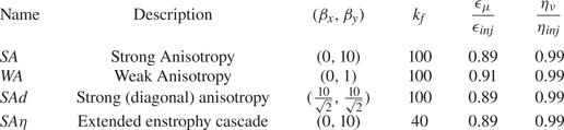
The parameters for the simulations are summarised in table 2. The simulations encompass varying anisotropy (through changing  $\boldsymbol {\beta }$) and forcing scales (
 $k_{inj}$). The use of hypo-viscosity, rather than linear drag, allows the development of an inverse energy cascade that spans a significant range of scales, but it increases the spin-up time for the simulations as the more energetic large scales take longer to reach equilibrium. To counter the long spin-up times, simulations are initially spun up at a lower resolution (
 $N=512$) until the large-scale energetics reach equilibrium. The higher-resolution (
 $N=2048$) simulations are initialised with the vorticity field of the
 $N=512$ simulations, linearly interpolated on to the appropriate grid, which preserves both the large-scale energetics and the vorticity at the grid scale of the
 $N=512$ model. The domain-integrated energy and enstrophy of the high-resolution simulations rapidly converges, and these simulations are run for 3000 s. In the strongly anisotropic simulations the large-eddy turnover time
 $T_e=E/\epsilon _{\mu } \approx 600$ meaning the statistics span approximately 5 large-eddy turnover times (
 $E$ is the domain-averaged energy). In the weak anisotropy simulations
 $T_e$ is shorter, but sensitivity tests (not shown) demonstrated that the results shown below are independent of whether the number and frequency of snapshots are adjusted based on
 $T_e$.
Description of important model parameters for each numerical experiment; the experiment name, a brief experiment description, the beta parameter in the  $x$- and
 $y$-directions, the forcing wavenumber
 $k_f$, the fraction of input energy being removed by large-scale hypo-viscosity (
 $\epsilon _{\mu }/\epsilon _{inj}$) and the fraction of input enstrophy being removed by small-scale hyper-viscosity (
 $\eta _{\nu }/\eta _{inj}$). All simulations have
 $N=2048$ grid-points in each direction, and are
 $3000$ s long with 60 evenly spaced snapshots.

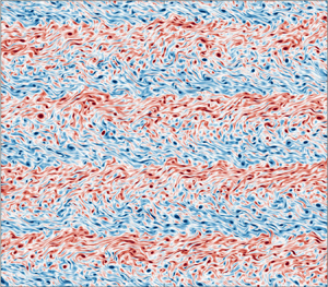
Snapshots of the vorticity at the end of each simulation are shown in figure 1 for one quarter of each domain. In the strongly anisotropic experiments ( $SA$,
 $SAd$ and
 $SA\eta$), jets form in the direction perpendicular to the
 $\boldsymbol {\beta }$-direction, consistent with previous studies of anisotropic 2-D turbulence (Danilov & Gryanik Reference Danilov and Gryanik2004; Kong & Jansen Reference Kong and Jansen2017). In contrast, the weakly anisotropic experiment (
 $WA$) does not develop jets and instead consists of seemingly isotropic vortices. The extended enstrophy cascade experiment (
 $SA\eta$) has a smoother vorticity field, consistent with larger-scale enstrophy driven by an increase in the energy/enstrophy injection scale
 $L_{inj}$.
Vorticity fields diagnosed from the final snapshot of each simulation. (a)  $SA$ experiment with a strong,
 $y$-aligned,
 $\beta$ term. (b)
 $WA$ experiment with a weak
 $y$-aligned
 $\beta$ term. (c)
 $SAd$ experiment with a strong diagonally aligned
 $\beta$ term. (d)
 $SA\eta$ experiment with an extended enstrophy cascade and a larger forcing scale. Vorticity values have been capped at
 $\pm 5 \ \textrm {s}^{-1}$ and are shown for one quarter of the domain for easier visualisation of small-scale features.

The external forces (beta effect, viscosity, etc.) acting on a fluid parcel are homogeneous in these simulations, but the presence of jets in the strong anisotropy simulations indicate that flow heterogeneity develops from the initially homogeneous flow (Bakas, Constantinou & Ioannou Reference Bakas, Constantinou and Ioannou2019). All the structure function relations in table 1 require an assumption of flow homogeneity in their derivation. These relations should still apply for the homogeneous scales smaller than the jets, that is  $r< W_{jet}$ where
 $W_{jet}$ is the along-
 $\boldsymbol {\beta }$ width of jets. There are roughly 20 jets in the domain of each strong anisotropy simulation, with a jet width
 $W_{jet} \approx {\rm \pi}/10$. This width is at the end of the inverse energy cascade (see next Section and figure 2), so we shall assume that the relations in table 1 are appropriate for the enstrophy and inverse energy cascades of the present simulations. It is possible that inhomogeneity affects these relations at the largest scales of the inverse energy cascade.
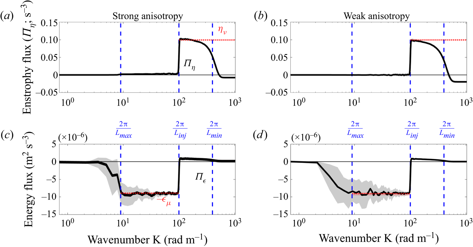
Spectral fluxes of enstrophy  $\varPi _{\eta }$ (a,b) and of energy
 $\varPi _{\epsilon }$ (c,d) for experiments with strong anisotropy (
 $SA$; a,c) and weak anisotropy (
 $WA$; b,d). Black lines show the mean fluxes, and shading shows the quartile range of these fluxes across the snapshots. Red dotted lines show (a,b) the mean rate of enstrophy dissipation by small-scale viscosity
 $\eta _{\nu }$, and (c,d) the mean rate of energy removal by large-scale hypo-viscosity
 $\epsilon _{\mu }$. Negative flux values imply a cascade to large scales (small-
 $K$), and positive values imply a cascade to small scales (large-
 $K$). Note that
 $\epsilon _{\mu }$ is positive definite, so negative
 $\epsilon _{\mu }$ is shown in the inverse energy cascade. Vertical blue lines denote the forcing wavenumber (
 $k_{inj}=2{\rm \pi} /L_{inj}$) and the diagnosed end of the inverse energy cascade (
 $2{\rm \pi} /L_{max}$).

3.1. Diagnostic tools
Structure functions, spectral fluxes, and dissipation rates are diagnosed from sixty evenly spaced snapshots of the flow field for each simulation. These statistics are then averaged across all snapshots, and their temporal variability is quantified by comparing the variations between the mean statistics diagnosed from each snapshot. The model velocity fields are used to calculate vorticity using a centred-difference estimate of gradients at the grid scale, and the advective derivatives are diagnosed using the same centred-difference method. These derivative estimates use a stencil width of one grid cell in either direction. The sensitivity of results to this stencil width are assessed in § 5.5. These are not exactly the derivatives used to solve prognostic equations, as the model uses spectral methods for advection.
Structure functions are calculated using separation vectors in specific directions; aligned with  $\boldsymbol {\beta }$ (along-
 $\boldsymbol {\beta }$), perpendicular to
 $\boldsymbol {\beta }$ (across-
 $\boldsymbol {\beta }$), and two diagonal directions (
 $\pm {\rm \pi}/4$ relative to the
 $\boldsymbol {\beta }$-axis). Using these different directional separations, the sensitivity of structure functions to sampling direction in anisotropic flows can be assessed. This directional dependence is important for observational analyses, which often utilise datasets with specific sampling patterns/directionality. Calculating structure functions in specific directions also reduces the computational cost of structure function calculations. Nie & Tanveer (Reference Nie and Tanveer1999) found that third-order structure functions are highly dependent on the sampling direction in anisotropic 3-D turbulence. Since the experiments use a doubly periodic domain, structure functions are diagnosed using only separations less than half the domain width, including separation vectors that ‘wrap around’ (through the periodic boundary). The sampling directions are chosen as they are with the eigenvectors of maximum and minimum anisotropy in the system (along and across
 $\beta$), and in directions in between these eigenvectors. Any anisotropy in structure function statistics would be captured by this set of sampling directions.
Spectral fluxes and dissipation rates are often challenging to calculate for observations and experiments, and for numerical simulations of complex domains, because they require spectrally transformable information about the full flow field (for fluxes), and about the smallest scales of the turbulent flow (for dissipation rates). The numerical simulations presented here provide an opportunity to calculate spectral fluxes, dissipation rates and structure functions from complete information about snapshots of the flow field, and to use these results to inform the analysis of situations where fluxes and dissipation results cannot be calculated.
The spectral fluxes of energy and enstrophy ( $\varPi _{\epsilon }$ and
 $\varPi _{\eta }$ respectively) are diagnosed for comparison. The spectral flux of enstrophy follows from the budget for the spectral enstrophy distribution [
 $\eta _k=\eta _k(\boldsymbol {k})=|\hat {\omega }|^{2}/2$ where
 $\boldsymbol {k}=(k,l)$ is the 2-D wavenumber vector]. To get to this budget we manipulate the Fourier transform of the vorticity budget ((2.1); transform denoted by a caret) and the budget for the complex conjugate of the transformed vorticity [
 $\hat {\omega }=\hat {\omega }(\boldsymbol {k})$],
 \begin{equation} \frac{\partial \eta_k}{\partial t} = \hat{\omega}^{*}\frac{\partial\hat{\omega}}{\partial t} + \hat{\omega}\frac{\partial \hat{\omega}^{*}}{\partial t} = T_{\eta} - D(k, \eta_k), \end{equation}
where  $T_{\eta }(\boldsymbol {k})=-Re[\hat {\omega }^{*}\widehat {\boldsymbol {u}\boldsymbol {\cdot } \boldsymbol {\nabla }\omega }]$ is the (spectral) divergence of the spectral flux of enstrophy between wavenumbers and
 $D(k, \eta _k)$ represents the removal of enstrophy by hypo- and hyper-viscosity. This enstrophy dissipation
 $D$ is assumed to occur at localised scales far from the forcing scale.
It then follows that the spectral flux of enstrophy into a specific region of  $\boldsymbol {k}$-space (
 $S_{\boldsymbol {k}}$) is
 \begin{equation} \varPi_{\eta}(k,l)=\iint\limits_{S_{\boldsymbol{k}}(k,l)}T_{\eta} \,\textrm{d}k\,\textrm{d}l. \end{equation}
In the present numerical simulations, this integral is evaluated in the region outside a circle of radius  $K$, that is
 $S_{\boldsymbol {k}}(k^{2}+l^{2}\geqslant K^{2})$. This results in the following spectral fluxes of enstrophy and energy respectively (Capet et al. Reference Capet, McWilliams, Molemaker and Shchepetkin2008),
 \begin{gather} \varPi_{\eta}(K)={\mathop{{\int\!\!\!\!\!\int}\mkern-21mu \bigcirc}\limits_{{k^{2}+l^{2}\geqslant K^{2}}}{Re\left[\hat{\boldsymbol{\omega}}^{*}\boldsymbol{\cdot}\widehat{\boldsymbol{u}\boldsymbol{\cdot}\boldsymbol{\nabla} \boldsymbol{u}}\right] \textrm{d}k\,\textrm{d}l}}\end{gather}
 \begin{gather}\varPi_{\epsilon}(K)={\mathop{{\int\!\!\!\!\!\int}\mkern-21mu \bigcirc}\limits_{{k^{2}+l^{2}\geqslant K^{2}}}{Re\left[\hat{\boldsymbol{u}}^{*}\boldsymbol{\cdot}\widehat{\boldsymbol{u}\boldsymbol{\cdot}\boldsymbol{\nabla} \boldsymbol{u}}\right] \textrm{d}k\,\textrm{d}l.}}\end{gather}
Positive fluxes indicate a transfer of energy/enstrophy to small scales (wavenumbers larger than  $K$), while negative values indicate transfer to large scales (wavenumbers smaller than
 $K$). While the present work uses these spectral fluxes between wavenumbers, it is also possible to diagnose real-space fluxes between different
 $r$ values for energy (Boffetta & Musacchio Reference Boffetta and Musacchio2010) and enstrophy (Chen et al. Reference Chen, Ecke, Eyink, Wang and Xiao2003).
Dissipation rates of energy and enstrophy are diagnosed in spectral space. The two dissipation rates of interest here, small-scale enstrophy ( $\eta _{\nu }$) and large-scale energy
 $\epsilon _{\mu }$ dissipation, were diagnosed as
 \begin{gather} \eta_{\nu} = \sum \nu K^{8}|\hat{\omega}|^{2} \end{gather}
 \begin{gather}\epsilon_{\mu} = \sum \mu K^{{-}4}|\hat{\omega}|^{2}, \end{gather}
where the summations are over all wavenumbers using Parseval's theorem (see Constantinou et al. Reference Constantinou, Wagner, Pearson, Karrasch and TagBot2020 for details). The other dissipation rates were calculated in an analogous manner.
The tools above diagnose the small- and large-scale dissipation rates and the presence of inertial cascades in isotropic wavenumber space. This is useful for applications where the transfer of properties by turbulence from one scale to another is of interest, but details of the mechanism of transfer are not relevant. In anisotropic flows where the full dynamic fields are measurable, it is possible to diagnose the anisotropic energy (or enstrophy) flux density using structure functions (Lamriben et al. Reference Lamriben, Cortet and Moisy2011) or spectral analysis (Yokoyama & Takaoka Reference Yokoyama and Takaoka2021). These anisotropic fluxes can provide information about the separate radial and angular transfers in these flows (e.g. Gomes-Fernandes et al. Reference Gomes-Fernandes, Ganapathisubramani and Vassilicos2015).
4. Fluxes and structure functions in anisotropic turbulence
4.1. Spectral fluxes of enstrophy and energy
Figure 2 shows the spectral fluxes of energy and enstrophy diagnosed from  $SA$ and
 $WA$ experiments (strong and weak anisotropy respectively). Positive fluxes indicate a transfer of energy/enstrophy to wavenumbers larger than
 $K$ (smaller scales), while negative values indicates transfer to smaller wavenumbers (larger scales). In both experiments the simulated turbulence develops a direct cascade of enstrophy to small scales and an inverse cascade of energy that spans almost an order of magnitude in scale, both originating at the forcing wavenumber.
The enstrophy fluxes  $\varPi _{\eta }$ to large wavenumbers agree with the rate of enstrophy dissipation at small scales
 $\eta _{\nu }$, and both
 $\varPi _{\eta }$ and
 $\eta _{\nu }$ have relatively small variations between snapshots. The enstrophy transfer to small wavenumbers is negligible [
 $\varPi _{\eta }(K < k_{inj})\approx -\eta _{\mu } \approx 0$]. Less than 1 % of injected enstrophy is dissipated by hypo-viscosity (table 2). The enstrophy cascade is estimated to end at a wavenumber associated with a minimum enstrophy cascade length scale
 $L_{min}=2{\rm \pi} /k_{min}$ (note
 $k_{min}$ is a maximum value, but is sub-scripted for consistency with
 $L_{min}$). This is estimated to be at a wavenumber bisecting the roll-off of the enstrophy cascade (figure 2). The transfer of energy to small wavenumbers, where it is removed by hypo-viscosity, is maintained by a negative energy flux
 $\varPi _{\epsilon }$ at wavenumbers smaller than the injection wavenumber
 $k_{inj}$. The spectral flux of energy is constant between the
 $k_{inj}$ and a wavenumber associated the maximum inverse cascade scale
 $L_{max} = 2{\rm \pi} / k_{max}$. The energy flux does not vary significantly between snapshots (denoted by the shading). This is indicative of a well-developed inverse kinetic energy cascade. The energy flux to small wavenumbers is approximated well by the rate of energy removal by hypo-viscosity (
 $\epsilon _{\mu }$). There is a small flux of energy to wavenumbers larger than
 $K$. This downscale energy flux is an order of magnitude smaller than the inverse cascade flux, and it agrees with the viscous dissipation rate of energy (
 $\epsilon _{\nu }$). Note that the fluxes should theoretically go to zero at the largest and smallest scales, but the enstrophy flux is non-zero at small scales. This is because the advective gradients in the spectral fluxes (i.e. (3.4)) are diagnosed in real-space using centered differences, rather than in the model's native spectral space, introducing truncation errors. The consistency of both fluxes with the dissipation rates
 $\epsilon _{\mu }$ and
 $\eta _{\nu }$ demonstrates that this noise does not significantly affect the fluxes in the inertial cascades.
The presence of a clear dual cascade in these simulations provides the opportunity to identify which structure functions are able to diagnose the dissipation rates of energy and enstrophy, and whether different types of structure functions have systematic biases or distinctions in their cascade estimates. We will first compare each of the structure functions against their expected behaviour based on theoretical considerations. Then, in § 5, the ability of different structure functions to predict the dissipation rates of energy and enstrophy will be assessed.
4.2. Vorticity-based structure functions
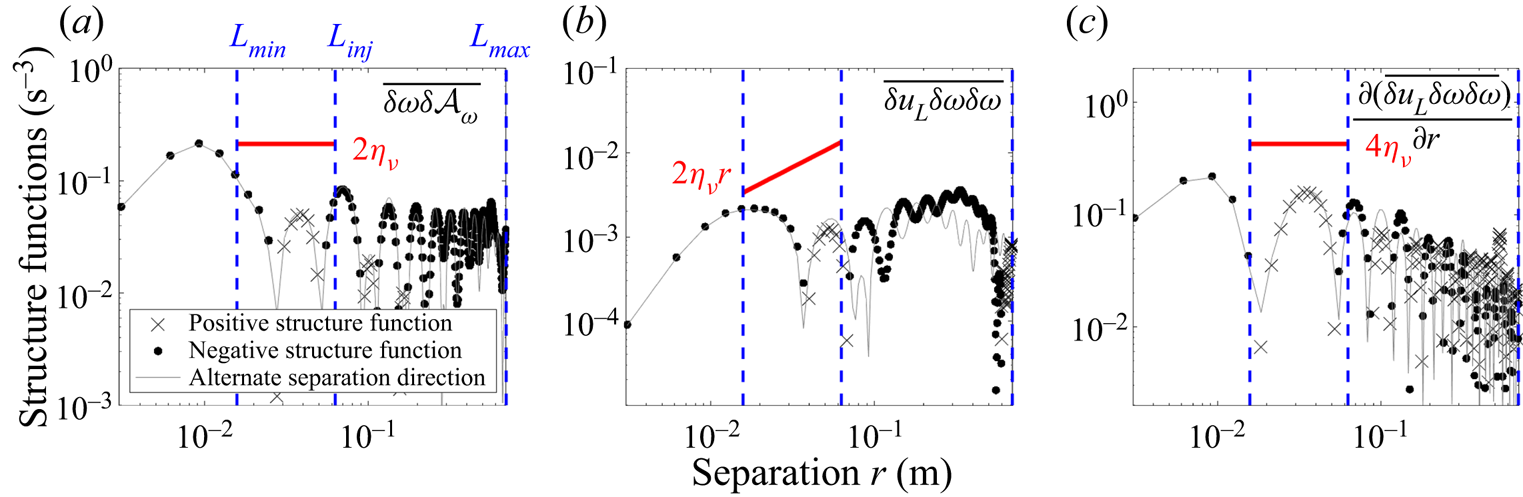
The vorticity-based structure functions in table 1 can theoretically diagnose the rate of enstrophy dissipation at small scales. Figure 3 shows the three vorticity-based structure functions from the  $WA$ experiment; the vorticity–advection structure function (2.8), the third-order vorticity/longitudinal velocity structure function (1.4a,b), and the divergence of this third-order structure function (1.5). The predictions for these structure functions, based upon these equations and the model-diagnosed rate of enstrophy dissipation
 $\eta _{\nu }$, are shown as red lines. These predictions span from the smallest scales of the enstrophy cascade
 $L_{min}$ to the energy injection scale
 $L_{inj}$. The advective structure function peaks at a value which is in good agreement with the enstrophy dissipation rate, while the other structure functions are always smaller than predicted. However, the region where each structure function is closest to its prediction occurs at scales just below
 $L_{min}$ rather than in the enstrophy cascade (note that the structure functions should be negative, that is, dots in the enstrophy cascade region). It will be shown in § 5.6 that the disagreement between these structure functions and their predictions within the enstrophy cascade are due to the finite width of the cascade. This suggests that the vorticity–advection structure function could be used to predict the enstrophy cascade rate provided these statistics are measured over a wide range of scales within, and smaller than, the enstrophy cascade region (see § 5). However, none of the structure functions follow the expected shape across the entire enstrophy cascade, and they all show a sign change at the largest scales of the enstrophy cascade. The divergence-based structure function in particular poorly captures the expected profile. The vorticity-based structure functions do not depend significantly on sampling direction, shown by the close agreement between symbols (along-
 $\boldsymbol {\beta }$ separations) and lines (across-
 $\boldsymbol {\beta }$ separations) across all
 $r$.
Vorticity-based structure functions plotted against separation distance for a simulation with weak anisotropy ( $WA$), and theoretical estimates of the structure functions diagnosed from the small-scale enstrophy dissipation rate (see legend and table 1). (a) shows the new vorticity-based advective structure function, (b) shows the third-order vorticity/longitudinal velocity structure function, and (c) shows the divergence of this third-order structure function. The sign of the along-
 $\boldsymbol {\beta }$ structure functions are denoted by symbol type, and the magnitude of the across-
 $\boldsymbol {\beta }$ structure functions are shown by the solid line to demonstrate anisotropic effects. The light solid line shows the magnitude of the structure functions diagnosed in the cross-
 $\boldsymbol {\beta }$ direction. Dashed blue lines show the energy injection scale (
 $L_{inj}$) and the maximum extent of the inverse energy cascade (
 $L_{max}$).

4.3. Velocity-based structure functions
The velocity-based structure functions are theoretically related to both the enstrophy cascade rate at small scales ( $r\ll L_{inj}$) and the inverse energy cascade rate at large scales (
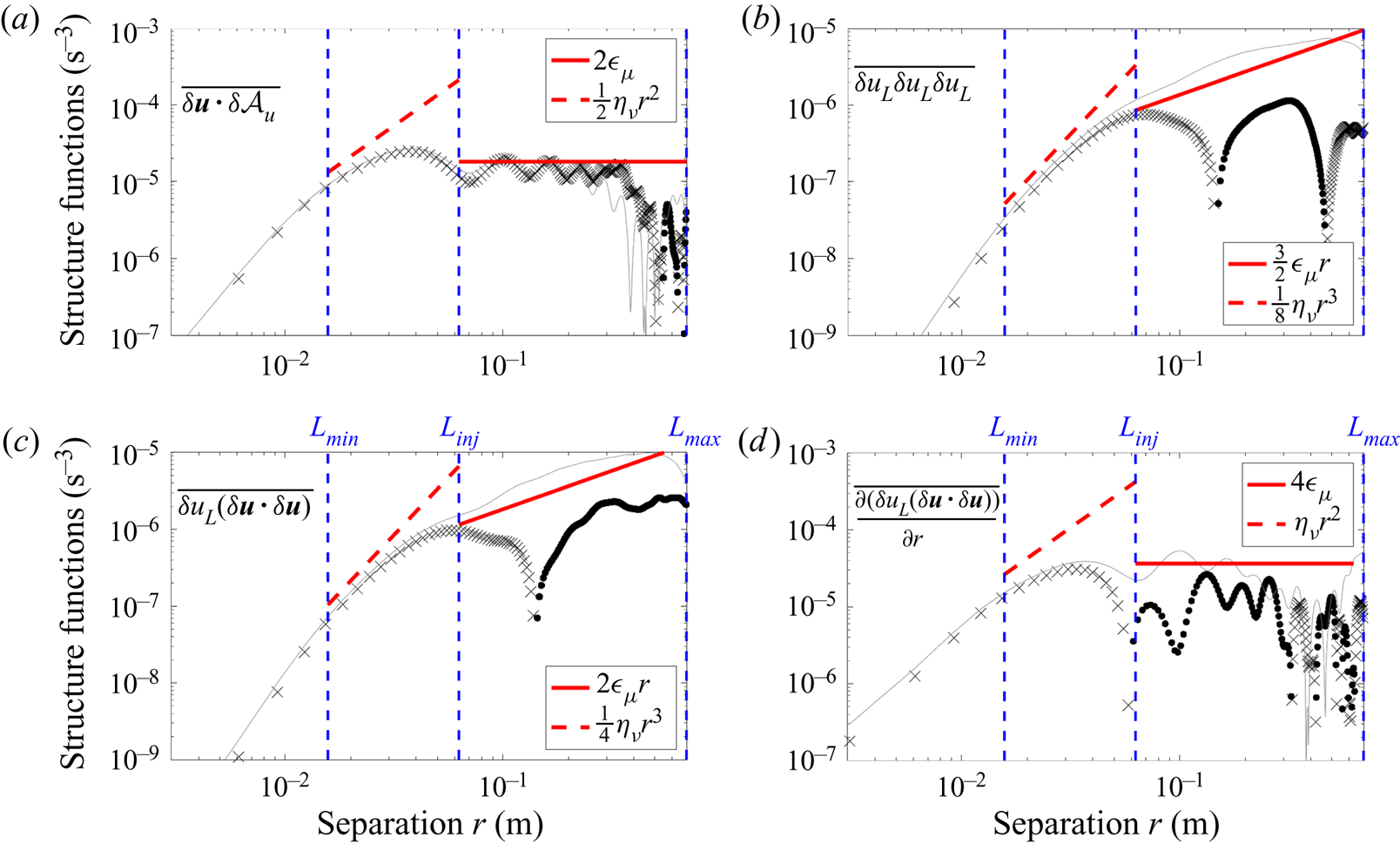
 $r\gg L_{inj}$) as summarised in table 1. Figure 4 shows the structure functions based on the velocity–advection (
 $\overline {\delta \boldsymbol {u}\boldsymbol {\cdot } \delta \boldsymbol {\mathcal {A}}_{\boldsymbol {u}}}$), the third-order longitudinal velocity (
 $\overline {\delta u_L \delta u_L \delta u_L}$), the third-order total velocity (
 $\overline {\delta u_L [\delta \boldsymbol {u}\boldsymbol {\cdot }\delta \boldsymbol {u}]}$) and the divergence of the third-order total velocity for the
 $WA$ experiment.
Velocity-based structure functions plotted against separation distance for a simulation with weak anisotropy ( $WA$), and theoretical estimates of the structure functions diagnosed from small-scale enstrophy and large-scale energy dissipation rates (see legend and table 1). (a) shows the new velocity-based advective structure function
 $\overline {\delta \boldsymbol {u}\boldsymbol {\cdot } \delta \boldsymbol {\mathcal {A}}_{\boldsymbol {u}}}$, (b) shows third-order longitudinal velocity structure function (
 $\overline {\delta u_L}\overline {\delta u_L}\overline {\delta u_L}$), (c) shows the third-order total velocity structure function (
 $\overline {\delta u_L \delta \boldsymbol {u}\boldsymbol {\cdot} \delta \boldsymbol {u}}$) and (d) shows the divergence of the third-order total velocity structure function. Other lines and symbols are as described in figure 3.

Across most of the inverse energy cascade ( $L_{inj} < r < L_{max}$), the advective structure functions shows good agreement with the
 $\epsilon _{\mu }$-based prediction (red solid line), and is not sensitive to the sampling direction. There is also clear oscillatory behaviour, which is related to the forcing scale and will be discussed in detail later (§ 5.6). Despite the experiment only having weak anisotropy, all the third-order structure functions depend significantly on sampling direction in the inverse cascade range. In the along-
 $\boldsymbol {\beta }$ direction, they do not follow the inverse cascade prediction, but in the cross-
 $\boldsymbol {\beta }$ direction they agree with the shape of the prediction but slightly overestimate its magnitude. The divergence of the third-order structure function has strong oscillations and typically lies below the predicted profile.
In the enstrophy cascade ( $r < L_{inj}$) all the structure functions approach, but underestimate, their predicted slopes for some scales
 $r < L_{inj}$. However, all of the structure functions steepen and move away from the predicted slope at the smallest scales. This steepening is most noticeable for the advective structure function. All of the velocity-based structure functions are relatively insensitive to sampling direction in the enstrophy cascade, and they all show a transition around
 $r=L_{inj}$, consistent with the discontinuous transition between
 $\epsilon _{\mu }$- and
 $\eta _{\nu }$-based predictions at this scale.
5. Estimating cascade rates in anisotropic 2-D turbulence
In this section the advective and third-order structure functions are used to estimate the dissipation rates of enstrophy and energy under strong anisotropy ( $SA$) and weak anisotropy (
 $WA$). The accuracy of these dissipation diagnostics is assessed, along with their sensitivity to the flow anisotropy and forcing scale, and the effects of the direction, frequency, and effective resolution of data sampling. For this section estimates from the divergent structure functions will not be considered, as the divergence calculation requires knowledge of flow anisotropy. In addition, the third-order total velocity structure function (
 $\overline {\delta u_L [\delta \boldsymbol {u}\boldsymbol {\cdot }\delta \boldsymbol {u}]}$) will not be used for diagnostics, as the results are similar to the more commonly used longitudinal-velocity structure function (figure 4). Estimates of dissipation rate are found by re-arranging each of the relations in table 1 to get an expression for the dissipation rates of enstrophy (
 $\eta _{\nu }$) or energy (
 $\epsilon _{\mu }$). These diagnostic expressions contain a structure function, a constant of proportionality, and, in some cases, a polynomial dependence on separation direction
 $r$.
5.1. Vorticity-based enstrophy cascade ($\eta _{\nu }$) estimates

Figure 5 shows estimates of the enstrophy dissipation rate from vorticity-based structure functions (blue and black lines) along with the model-diagnosed  $\eta _{\nu }$ (red line). All the estimates show little variability between snapshots (shading shows the quartiles of the along-
 $\boldsymbol {\beta }$ estimate). The vorticity–advection structure function peaks close to
 $\eta _{\nu }$, regardless of the sampling direction, even under conditions of strong anisotropy. In contrast, the vorticity-based third-order structure function is extremely sensitive to the sampling direction under strongly anisotropic conditions. In experiment
 $SA$ the along- and across-
 $\boldsymbol {\beta }$ directions significantly underestimate
 $\eta _{\nu }$, while the intermediate directions peak close to
 $\eta _{\nu }$. While some of the vorticity-based structure functions peak close to
 $\eta _{\nu }$, none of the structure functions stay near
 $\eta _{\nu }$ across all the enstrophy cascade, and this difference is most noticeable just below the forcing scale
 $L_{inj}$. All the structure functions oscillate, although these oscillations are less noticeable at large scales for third-order structure functions diagnostics due to their inverse
 $r$ dependence. In § 5.6 it is shown that the oscillations and the peaking rather than plateauing nature of the structure function
 $\eta _{\nu }$ estimates, are coupled to the forcing scale and the limited width of the inertial enstrophy cascade respectively. Note that the discretised grid means that the smallest separation distance in the diagonal directions is
 $\sqrt {2}$ larger than the smallest separation distance in the along-
 $\beta$ and across-
 $\beta$ directions.
Small-scale enstrophy dissipation rate and estimates of this rate from vorticity-based structure functions for the strongly anisotropic ( $SA$; a,c) and weakly anisotropic (
 $WA$; b,d) simulations. The top panels shows estimates using the new vorticity–advection structure function
 $\delta \omega \delta \mathcal {A}_{\omega }$ and the diagnosed dissipation rate (
 $\eta _{\nu }$; red dashed line). These
 $\eta _{\nu }$ estimates are diagnosed from structure functions calculated in specific directions denoted by line colour and style. Shading denotes the quartile spread across snapshots of the along-
 $\beta$ estimate. The bottom panels are analogous to the top panels but use the third-order blended vorticity structure function
 $\delta u_L \delta \omega \delta \omega$. Blue dashed lines denote the energy/enstrophy injection scale (
 $L_{inj}$) and the largest scale of the inverse energy inertial cascade (
 $L_{max}$).

5.2. Velocity-based enstrophy cascade ($\eta _{\nu }$) estimates

Figure 6 shows estimates of the enstrophy dissipation rate from velocity-based structure functions (blue and black lines) along with the model-diagnosed  $\eta _{\nu }$ (red line). The variability of
 $\eta _{\nu }$ estimates between snapshots is reduced as the anisotropy increases, perhaps due to the reduced dimensionality of the system. The velocity–advection structure function underestimates
 $\eta _{\nu }$ by approximately 30 % at its peak. The advective structure function also shows little sensitivity to sampling direction, even under strongly anisotropic conditions. In contrast, the third-order structure function estimate depends greatly on sampling direction; the across-
 $\boldsymbol {\beta }$ sampling produces estimates that are an order of magnitude smaller than
 $\eta _{\nu }$ for all
 $L_{min} < r < L_{inj}$, while the along-
 $\boldsymbol {\beta }$ and intermediate sampling directions produce peaks close to
 $\eta _{\nu }$. Under weakly anisotropic conditions, all the third-order structure function estimates peak within the same order as
 $\eta _{\nu }$, although there is substantial variability between snapshots. The variability of the advective structure functions is smaller, and hence the statistical convergence is faster, than for the third-order structure functions. The underestimation of
 $\eta _{\nu }$ under strong anisotropy is likely due to the forcing scale and limited width of the enstrophy cascade, as discussed in § 5.6.
Small-scale enstrophy dissipation rate ( $\eta _{\nu }$) and estimates of this rate from velocity-based structure functions. This is analogous to figure 5 but using velocity-based advective and third-order structure functions (
 $\delta \boldsymbol {u}\boldsymbol {\cdot } \delta \boldsymbol {\mathcal {A}_u}$ and
 $\delta u_L\delta u_L\delta u_L$ respectively) rather than vorticity-based structure functions.

5.3. Velocity-based energy cascade ($\epsilon _{\mu }$) estimates

Figure 7 shows estimates of the large-scale energy dissipation rate ( $\epsilon _{\mu }$) from velocity-based structure functions (blue and black lines) along with the model-diagnosed
 $\epsilon _{\mu }$ (red line). The energy dissipation estimates should apply at large scales (
 $L_{max}>r>L_{inj}$; between the vertical dashed lines). The variability of estimates between snapshots are large and plotted separately in figure 8.
Large-scale energy dissipation rate (red line) and estimates of this rate from velocity-based structure functions. This is analogous to the previous two figures except the focus is now on separation distances in the inverse energy cascade ( $L_{inj} < r < L_{max}$), and the associated rate of energy removal by hypo-viscosity (
 $\epsilon _{\mu }$; red dashed line).

A zoomed-out version of figure 7 that includes the temporal variability of the estimates of large-scale energy dissipation rate. Shading shows the quartile spread across snapshots for each sampling direction. Note that only one diagonal direction is shown for clarity.

The estimates based on velocity–advection structure functions closely follow, albeit oscillate about,  $\epsilon _{\mu }$ near the forcing scale
 $L_{inj}$. At larger scales it underestimates
 $\epsilon _{\mu }$ in both weak and strong anisotropy, except in the direction of jets for the strong anisotropy (
 $SA$) experiment, where the dissipation estimate is fairly accurate to the end of the inverse cascade at
 $L_{max}$. This sampling anisotropy is a real signal, because the variability of estimates between snapshots (top left panel of figure 8) is also distinct and relatively narrow for each direction. These structure functions have clear oscillatory behaviour, which is discussed further in § 5.6.
The  $\epsilon _{\mu }$ estimates based on third-order structure functions are highly sensitive to sampling direction. In the strong anisotropy (
 $SA$) experiment, the along- and across-
 $\boldsymbol {\beta }$ estimates persistently underestimate the energy dissipation with little variability between snapshots, while the diagonal estimates have large variability and go from overestimating
 $\epsilon _{\mu }$ near
 $L_{inj}$ to underestimating it near
 $L_{max}$. The temporal variability of the diagonal estimates increases with separation distance, even with the inverse
 $r$ dependence of the estimate. In the weak anisotropy case, the third-order structure functions estimates also vary with sampling direction. All the estimates, except along-
 $\boldsymbol {\beta }$, plateau through the energy cascade, but they all predict different magnitudes for
 $\epsilon _{\mu }$. Unlike the strong anisotropy case, under weakly anisotropic conditions the inter-snapshot variability of third-order-based estimates are similar in all directions.
The results suggest that velocity–advection structure functions can provide estimates of large-scale energy dissipation rates in 2-D turbulence, even under strong anisotropy. These estimates are particularly accurate just above the forcing scale, regardless of sampling direction or flow anisotropy. The forcing scale could potentially be diagnosed from oscillations in structure functions (see § 5.6). In contrast, estimates based on the third-order longitudinal structure function are less useful for predicting  $\epsilon _{\mu }$ as they have larger variability between snapshots, are more sensitive to the sampling direction, and do not generally align with
 $\epsilon _{\mu }$. These drawbacks are amplified as flow anisotropy increases.
5.4. Intermittency of velocity-based structure functions
It was shown previously that the velocity-based advective structure function has less temporal variability than the third-order structure function (figures 6 and 8). At first glance this may seem counter-intuitive as the advective structure function contains local gradients of velocity, which are typically noisier than the raw velocity field used for the third-order structure function. However, there are two properties of the advective structure function that could explain its lower variability relative to the third-order structure function. First, the gradients of turbulent velocities are constrained by the 2-D dynamics of the system through the vorticity budget and incompressibility. This could provide a mechanism for intermittency in any of the four derivatives of the advective structure function to be compensated by intermittency in the other derivatives ( $\partial _x u$,
 $\partial _x v$,
 $\partial _y u$ and
 $\partial _y v$). Second, the advective structure function contains one less increment than the third-order structure function. These increments could introduce variability due to flow intermittency (i.e.
 $\delta u_L \sim [\partial _r u_L] \delta r$). The present simulations provide an ideal test bed to compare these mechanisms because the velocity fields used to diagnose structure functions are exact, while the velocity gradients contain noise relative to what the model ‘sees’. This is because we directly use the model's velocity field but estimate gradients and vorticity by applying finite-difference methods to this velocity field, rather than using the model's native spectral derivatives, resulting in truncation errors (see § 3).
Figure 9 shows p.d.f.s of the velocity-based structure functions from a snapshot of experiment  $WA$ for three
 $x$-separations spanning the enstrophy cascade, the forcing scale, and the inverse energy cascade. These figures are analogous to velocity-increment p.d.f.s (i.e. Boffetta & Musacchio Reference Boffetta and Musacchio2010; Poje et al. Reference Poje, Özgökmen, Bogucki and Kirwan2017), except that the present figures show p.d.f.s of increment products in order to compare the advective and third-order structure functions. The structure functions are normalised by their standard deviation across this snapshot at that separation, so that the relative contribution of their tails can be compared. Wider-tailed distributions indicate increased spatial intermittency of the increment-products, which suggests more data would be required for an accurate estimate of its average (for the relations in table 1). At all scales, the advective structure function has narrower tails (lower spatial variability/intermittency) than the third-order structure function. This suggests that advective structure functions require less data to get an accurate estimate of their mean value than third-order structure functions require.
Probability distribution functions (p.d.f.s) of velocity-based third-order (red) and advective (black) structure functions in the weak anisotropy ( $WA$) simulation. Probability distribution functions are shown for
 $x$-aligned separation vectors (a) in the enstrophy cascade, (b) at the forcing scale, and (c) in the inverse energy cascade. The structure functions are calculated at all points in the domain and normalised by their respective standard deviation [
 $\delta \boldsymbol {u}\boldsymbol {\cdot } \delta \boldsymbol {\mathcal {A}_u}/std(\delta \boldsymbol {u}\boldsymbol {\cdot } \delta \boldsymbol {\mathcal {A}_u})$,
 $\delta u_L^{3}/std(\delta u_L^{3})$, etc.]. Also shown are the components of the advective structure function arising from
 $x$- and
 $y$-oriented increments (dotted and dashed lines respectively). Probability distribution functions were diagnosed from the final snapshot of the
 $WA$ simulation.

Figure 9 also shows p.d.f.s of the  $x$- and
 $y$-components of the advective structure function (
 $\overline {\delta u\delta \mathcal {A}_u}$ and
 $\overline {\delta v\delta \mathcal {A}_v}$) to test whether the small spatial intermittency of
 $\overline {\delta \boldsymbol {u}\boldsymbol {\cdot }\delta \boldsymbol {\mathcal {A}_u}}$, relative to
 $\delta u_L \delta u_L \delta u_L$, is due to compensation between advective gradients or the reduced number of increments. The two components of the advective structure function have large tails, similar to the third-order structure function. This demonstrates that the lower variability of the advective structure function relative to the third-order structure function is a result of compensation between gradients in the
 $\overline {\delta u\delta \mathcal {A}_u}$ and
 $\overline {\delta v\delta \mathcal {A}_v}$ components of the structure function.
5.5. Impact of effective resolution of derivatives
Many of the structure functions discussed above require gradients of flow properties because they contain advective operators ( $\overline {\delta \boldsymbol {u}\boldsymbol {\cdot }\delta \boldsymbol {\mathcal {A}}_{\boldsymbol {u}}}$), vorticity (
 $\delta u_L \delta \omega \delta \omega$) or both (
 $\overline {\delta \omega \boldsymbol {\cdot }\delta \mathcal {A}_{\omega }}$). These gradients were estimated using a centred-difference approximation and the adjacent grid points, with a ‘stencil width’ of 2 grid points. This is the smallest centred stencil that can be used to estimate gradients at a grid point, which means the derivative is calculated at the smallest scales of the simulated turbulence. In general, data from turbulent flows are not at the smallest scales of turbulence so any derivative calculations using this data could be affected by the presence of sub-stencil turbulence.
To assess the impact of stencil width and the presence of sub-stencil turbulence on the structure functions, the advective and vorticity-based structure functions were recalculated from a snapshot of the  $SA$ experiment where derivatives (vorticity and advection) were diagnosed using centred-differences with varying stencil widths (2, 4, 6 and 8 grid points). These derivatives all use two data points, for example the 8 grid cell stencil only uses the two grid points that are
 $\pm$4 adjacent to the derivative location. Figure 10 shows the structure functions diagnosed with different stencil widths. At large scales the structure functions are relatively unaffected by stencil width, but at small scales the vorticity-containing structure functions the maximum/minimum values are sensitive to stencil width, suggesting that their estimates of enstrophy dissipation (figure 5) will vary with the effective resolution of data and the properties of turbulence at scales smaller than this resolution. The velocity–advection structure function is not significantly affected by stencil width at the scales used to estimate enstrophy and energy dissipation rates, and is only changed at small scales where the increased stencil width increases the magnitude of the structure function at the smallest scales.
Comparison of structure functions using different stencil widths for derivative calculations: (a) velocity–advection structure function, (b) velocity–advection structure function scaled by  $r^{2}$, (c) vorticity–advection structure function and (d) third-order vorticity structure function scaled by
 $r$, for centred-difference stencil widths of 2, 4, 6 and 8 grid cells. The left-most panel is an inverse energy cascade diagnostic, while the other three panels are enstrophy cascade diagnostics (table 1). The vertical dashed lines denote the energy/enstrophy injection scale
 $L_{inj}$ and the end of the enstrophy cascade
 $L_{min}$.

5.6. Effect of forcing scale and enstrophy cascade width
The structure function relations presented in table 1 are derived for the inertial cascades of 2-D turbulence. The experiments presented above ( $SA$ and
 $WA$) have inverse energy cascades that span an order of magnitude in scale, but their enstrophy inertial cascades are narrower. To investigate the importance of the enstrophy cascade width an experiment was conducted under strong anisotropic conditions like experiment
 $SA$, but with forcing at a larger scale (
 $k_{inj}=40$). A second motivation for this experiment is that several of the dissipation estimates and structure functions show oscillatory or peaked behaviour, implying that an external length scale is affecting the statistics. As the only imposed length scales are the forcing scale
 $L_{inj}$ and the numerical grid properties, this experiment can be used to diagnose whether these structure function features are driven by the physical parameters this system or the numerics/resolution.
Figure 11 shows the spectral enstrophy flux in this extended enstrophy cascade experiment ( $SA\eta$) alongside the flux from the
 $SA$ experiment. The fluxes are normalised by the enstrophy injection rate at their respective forcing scales. Experiment
 $SA\eta$ produces an well-developed and wide enstrophy cascade, where the enstrophy flux is flat across a much wider range of scales than the other experiments. The variability of the spectral fluxes between snapshots is small indicating that the inertial cascades are statistically stationary.
Normalised spectral fluxes of enstrophy  $\varPi _{\eta }/\eta _{\nu }$ for experiments with an extended enstrophy cascade (
 $SA\eta$; solid line) or a short enstrophy cascade (
 $SA$; dashed line). Both simulations have strong anisotropy. From left to right the vertical blue lines denote the forcing wavenumbers of the
 $SA\eta$ and
 $SA$ simulations, and the maximum wavenumber of the enstrophy cascade
 $2{\rm \pi} /L_{min}$ and shading denotes the temporal variability of the fluxes across snapshots (see figure 2 for details).

The impacts that changing the forcing scale has on enstrophy dissipation estimates are shown in figures 12 and 13, which compare vorticity-based and velocity-based estimates of  $\eta _{\nu }$, respectively, between experiments
 $SA\eta$ and
 $SA$. These estimates are scaled by the model-diagnosed
 $\eta _{\nu }$ which varies between the simulations. The vorticity-based
 $\eta _{\nu }$ estimates (figure 12) are comparable in both simulations.
Vorticity structure function-based estimates of small-scale enstrophy dissipation rate (normalised by actual rate  $\eta _{\nu }$) from an anisotropic 2-D simulation with an extended enstrophy cascade (
 $SA\eta$; a,c) and from a simulation with a short enstrophy cascade (
 $SA$; b,d). Note that the forcing scale
 $L_{inj}$ denoted by the blue dashed line differs between the simulations. Linestyles denote sampling direction and shading denotes temporal variability (see figure 5).

Velocity structure function-based estimates of small-scale enstrophy dissipation rate (normalised by actual rate  $\eta _{\nu }$) from an anisotropic 2-D simulation with an extended enstrophy cascade (
 $SA\eta$; a,c) and from a simulation with a short enstrophy cascade (
 $SA$; b,d). Linestyles denote sampling direction and shading denotes temporal variability as in figure 5.

In a wider enstrophy cascade, the velocity-based advective structure function becomes an even better estimator of  $\eta _{\nu }$. It plateaus close to the model-diagnosed
 $\eta _{\nu }$ throughout most of the enstrophy cascade region (
 $L_{min} < r < L_{inj}$). Below the enstrophy cascade (
 $r < L_{min}$) and near the forcing scale the velocity-based structure function becomes smaller than
 $\eta _{\nu }$. In contrast, the third-order velocity-based estimates become even more sensitive to the sampling direction as
 $L_{inj}$ increases and the enstrophy cascade becomes wider. The velocity–advection structure functions are a useful tool for diagnosing dissipation rates for several reasons discussed previously, and these
 $SA\eta$ experiment results suggest that the accuracy of its estimates increases with the width of the inertial cascade.
Another important result of the  $SA\eta$ experiment is that the oscillations and peaked behaviour of the dissipation estimates are governed by the forcing length scale
 $L_{inj}$ rather than the numerical properties of the experiments. For example, the wavelength of oscillations in
 $\delta \omega \delta \mathcal {A}_{\omega }$ (figure 12a,b) become wider as
 $L_{inj}$ increases. In fact, the oscillations appear to have a wavelength that is approximately
 $L_{inj}$, as the second zero-crossing lies close to
 $L_{inj}$ in both experiments. This could provide a method to estimate the forcing scale of 2-D flows using structure function measurements across a range of scales. This wavenumber is independent of the sampling direction even under the strong anisotropy of this system. Similar behaviour is seen in the oscillations and humps of
 $\delta u_L \delta \omega \delta \omega$ and
 $\delta \boldsymbol {u} \boldsymbol {\cdot } \delta \boldsymbol {\mathcal {A}}_{\boldsymbol {u}}$ respectively, although this is less noticeable owing to the inverse dependence of these estimates on separation distance. This oscillatory behaviour could be related to the finite width of the inertial cascade, and the presence of a dual cascade in this system. Xie & Bühler (Reference Xie and Bühler2018) propose relations between third-order structure function and energy dissipation rates in dual-cascading isotropic 2-D turbulence that contain Bessel functions with wavenumber
 $k_{inj}$. Their relations were validated in an isotropic magneto-hydrodynamic system with dual cascades of energy, and could be a fruitful direction for extending advective structure function theory to explain this oscillatory behaviour. Taking inspiration from Xie & Bühler (Reference Xie and Bühler2018), the oscillations of
 $\delta \boldsymbol {u} \boldsymbol {\cdot } \delta \boldsymbol {\mathcal {A}}_{\boldsymbol {u}}$ seen in the inverse energy cascade of figures 7 and 13 (the oscillations are scaled by
 $r^{2}$ in the latter) can be better approximated by modifying the dissipation in the relations of table 1 by
 $\epsilon _{\mu }\rightarrow \epsilon _{\mu }[1-0.5(L_{inj}/r)\cos (Ar/L_{inj})]$ where
 $A\approx 7$ (not shown).
5.7. Effect of anisotropy direction
In the experiments used to find the above results ( $SA$,
 $WA$ and
 $SA\eta$), the anisotropy vector (
 $\boldsymbol {\beta }$) is aligned with numerical grid. To demonstrate that the variations in structure function-based dissipation estimates with the sampling direction is driven by physics, rather than the numerical grid orientation, an additional experiment (
 $SAd$) was carried out where
 $\boldsymbol {\beta }$ is aligned with the diagonal direction (specifically it is rotated
 ${\rm \pi} /4$ from the numerical grid orientation). In figure 14, all the estimates of enstrophy and energy dissipation from experiment
 $SAd$ are contrasted against those from experiment
 $SA$. Line styles are chosen so that the same lines in the top panels (
 $SA$) and bottom panels (
 $SAd$) have the same orientation relative to
 $\boldsymbol {\beta }$. From this figure it is clear that the estimates of dissipation rates, and therefore the structure functions and their directional dependency, are driven by the
 $\boldsymbol {\beta }$ orientation rather than the numerical grid orientation.
Comparison of dissipation estimates between the strongly anisotropic simulations with meridionally and diagonally aligned  $\beta$ terms (experiments
 $SA$ and
 $SAd$ respectively). Dissipation estimates from all advective and third-order structure functions are shown. The top panels show the meridionally aligned
 $\beta$ experiment whereas the bottom panels show the diagonally aligned
 $\beta$ experiment. Line styles are based on sampling orientation relative to
 $\beta$ so that the same lines are comparable between the top and bottom panels. Note the structure functions and their anisotropy are essentially independent of the numerical grid orientation.

6. Utility of new relations
The results were derived from the vorticity budget with only viscous damping (2.1), assuming that the scales of interest are in an inertial cascade. The ability of structure functions to diagnose dissipation rates in more complex 2-D flows, as demonstrated previously, is encouraging. In particular, the success of advective structure functions to diagnose energy and enstrophy cascade rates, in anisotropic, forced 2-D turbulence with large- and small-scale dissipation expands the breadth of practical scenarios where these relations could be applied. Our results extend beyond previous studies which have shown that, in isotropic 2-D turbulence, external forcing at a specific scale does not affect third-order structure function relations within the inertial cascades (Lindborg Reference Lindborg1999; Cerbus & Chakraborty Reference Cerbus and Chakraborty2017), and similar results for 3-D turbulence (Banerjee & Galtier Reference Banerjee and Galtier2016). Cerbus & Chakraborty (Reference Cerbus and Chakraborty2017) suggested that large-scale dissipation would reduce the down-scale enstrophy cascade rate  $\epsilon _{\omega }$ as some enstrophy will be removed by large-scale drag or hypo-viscosity. In the present simulations, approximately 99 % of enstrophy is dissipated at small scales, and approximately 90 % of energy is dissipated at large scales (table 2).
Despite the success of advective structure functions as diagnostics for dissipation rates in the above experiments, there are differences that likely arise from the complexity of the flow and the simplifying assumptions in the derivations. In forced-dissipative 2-D turbulence, the accuracy of the new relations in table 1 could be increased if additional physical properties are considered. For example, the structure functions at a given separation  $r$ within an inertial range could be affected by non-local dynamics at other
 $r$, such as forcing and the other inertial cascade (in a dual cascading system). Third-order structure function laws have been proposed for isotropic 2-D turbulence that apply outside idealised inertial cascades (Xie & Bühler Reference Xie and Bühler2018, Reference Xie and Bühler2019). It is possible that the derivations presented here could also be modified to extend outside of inertial ranges, such as near the forcing scale or in regions of overlapping energy and enstrophy cascades (Lindborg Reference Lindborg1999; Thompson & Young Reference Thompson and Young2006; Cerbus & Chakraborty Reference Cerbus and Chakraborty2017). The relationship shown in (2.9) means that any extant laws containing
 $\boldsymbol {\nabla }_r\boldsymbol {\cdot }(\overline {\delta \boldsymbol {u}\delta \omega \delta \omega })$ can be converted into laws in terms of
 $\overline {\delta \omega \delta \mathcal {A}_\omega }$, and similarly the relation
 $\overline {\delta \boldsymbol {u} \boldsymbol {\cdot } \delta (\boldsymbol {u}\times \boldsymbol {\omega })}=-(1/2) \boldsymbol {\nabla }_r\boldsymbol {\cdot }(\overline {\delta \boldsymbol {u}[\delta \boldsymbol {u} \boldsymbol {\cdot }\delta \boldsymbol {u}])}$ allows the conversion of extant laws with third-order velocity structure functions into laws with second-order structure functions. Together these relations can convert the previously referenced results into second-order structure function laws in isotropic 2-D turbulence, but their extension to anisotropy would require more considered derivations.
6.1. Potential for practical applications of advective structure functions
Third-order structure functions have previously been used to study the dynamics of the atmosphere and ocean (Cho & Lindborg Reference Cho and Lindborg2001; Deusebio et al. Reference Deusebio, Augier and Lindborg2014; Balwada, LaCasce & Speer Reference Balwada, LaCasce and Speer2016; Poje et al. Reference Poje, Özgökmen, Bogucki and Kirwan2017; Pearson et al. Reference Pearson, Fox-Kemper, Pearson, Chang, Haus, Horstmann, Huntley, Kirwan, Lund and Poje2020) as well as other planets (Young & Read Reference Young and Read2017). However, making appropriate measurements of flow properties can be challenging owing to the nature and uncertainty of both in situ and remote data collection (LaCasce Reference LaCasce2008; Chang et al. Reference Chang2019; Pearson et al. Reference Pearson, Fox-Kemper, Barkan, Choi, Bracco and McWilliams2019). The predictions of dissipation rates from advective structure functions have less variability between snapshots, and are relatively insensitive to sampling direction, when compared with predictions from third-order structure functions. These are both important considerations when analyzing real datasets which have specific sampling patterns and finite measurements. The caveat of the advective structure functions is that they require the calculation of the derivatives of flow properties, as do the vorticity-based structure functions. For some geophysical measurement techniques, such as aircraft-track data (Lindborg Reference Lindborg1999; Deusebio et al. Reference Deusebio, Augier and Lindborg2014), this information is not available and the advective structure functions may not be diagnosed. However, there are many current and future datasets where sufficient information is available to diagnose the new structure functions. For example in the ocean, platforms that can diagnose vorticity and gradients include surface drifter deployments (Ohlmann et al. Reference Ohlmann, Molemaker, Baschek, Holt, Marmorino and Smith2017), radar observations (Pearson et al. Reference Pearson, Fox-Kemper, Pearson, Chang, Haus, Horstmann, Huntley, Kirwan, Lund and Poje2020), gridded satellite observations (Khatri et al. Reference Khatri, Sukhatme, Kumar and Verma2018), and satellites that observe 2-D swaths of the ocean, including upcoming satellite campaigns (Zaron & Rocha Reference Zaron and Rocha2018). Numerical simulations also provide the necessary variables to diagnose the new structure functions. Global-scale numerical simulations can presently resolve large-scale turbulence in both the atmosphere and ocean (Pearson et al. Reference Pearson, Fox-Kemper, Bachman and Bryan2017), and analyses of cascade rate statistics in these simulations, which could be inferred from structure functions, can improve our physical understanding of these systems (e.g. Pearson & Fox-Kemper Reference Pearson and Fox-Kemper2018). The velocity-based advective structure function shows the greatest potential for these practical applications, as it is not sensitive to the details of the derivative calculation, or the presence of turbulence at scales smaller than the derivative calculation (which exists in observations).
7. Conclusions
New relations were derived between advective structure functions ( $\delta \boldsymbol {u} \boldsymbol {\cdot } \delta \boldsymbol {\mathcal {A}}_{\boldsymbol {u}}$ and
 $\delta \omega \delta \mathcal {A}_{\omega }$; see table 1), and the cascade rates of energy and enstrophy in 2-D turbulence. Numerical simulations of anisotropic 2-D turbulence demonstrated that different structure function methods to estimate cascade rates have varying levels of accuracy. The new advective structure functions were shown to be powerful tools for estimating cascade rates, as they are not significantly affected by flow anisotropy, background currents and vorticity, or sampling direction. The advective structure functions also have lower temporal and spatial variability relative to third-order structure functions, leading to more accurate structure function estimates with finite sampling. In contrast, traditional third-order structure function methods are poor estimators for cascade rates in anisotropic 2-D turbulence as they are affected by the details of flow anisotropy and sampling. The velocity-based advective structure functions show particular promise for diagnosing both enstrophy and inverse energy cascade rates in 2-D turbulence, when compared with vorticity-based advective structure functions and third-order structure functions. An extended enstrophy cascade simulation and rotated anisotropy simulation are used to demonstrate that the results are robust to the numerics of the simulations and the finite width of the inertial cascades, although the accuracy of dissipation rate estimates from structure functions increases with the width of the inertial cascade. The velocity-based advective structure functions are even more useful if the forcing scale of the system is already known. Preliminary results suggest that this scale could also be diagnosed from the structure functions. Advective structure functions depend on local gradients of velocity. As a result, they can be calculated in numerical models and many existing/future observations. However, the advective structure functions cannot be applied to observations where information is only known in one direction, with the exception of
 $\overline {\delta \boldsymbol {u}\boldsymbol {\cdot } \delta \boldsymbol {\mathcal {A}}_{\boldsymbol {u}}}$ which could be diagnosed in the special case where the 1D track is in the same direction as the flow velocity.
Acknowledgements
Funding from ONR N00014-17-1-2963 and NSF award number 2023721 is gratefully acknowledged.
Declaration of interests
The authors report no conflict of interest.
Appendix A. Coordinate transformations
The derivation of the correlation equations and structure function relationships requires a coordinate transformation to relative coordinates,  $\boldsymbol {r}$ and
 $\boldsymbol {x}_0$, from the Navier–Stokes equation coordinates,
 $\boldsymbol {x}=\boldsymbol {x}_0$ and
 $\boldsymbol {x}'=\boldsymbol {x}_0+\boldsymbol {r}$. This transformation can be derived from the total derivative of a function
 $f=f(\boldsymbol {x},\boldsymbol {x}')=f(\boldsymbol {x}_0,\boldsymbol {r})$ (for simplicity we assume differences in an arbitrary direction and drop vector notation)
 \begin{equation} \textrm{d}f= \left(\frac{\partial f}{\partial x}\right)_{x'}{\textrm{d} x} + \left(\frac{\partial f}{\partial x'}\right)_{x}{\textrm{d} x}' = \left(\frac{\partial f}{\partial x_0}\right)_{r}\,\textrm{d}x_0 + \left(\frac{\partial f}{\partial r}\right)_{x_0}\,\textrm{d}r, \end{equation}
where subscripts on parentheses denote variables that are held constant and  $\textrm {d}f$ denotes the total differential of
 $f$. It then follows that, if
 $x$ is varied while
 $x'$ is held constant (
 ${\textrm {d} x}'=0=\textrm {d}x_0+\textrm {d}r$ and
 ${\textrm {d} x}=\textrm {d}x_0$) then,
 \begin{equation} \left(\frac{\partial f}{\partial x}\right)_{x'} =\left(\frac{\partial f}{\partial x_0}\right)_{r} - \left(\frac{\partial f}{\partial r}\right)_{x_0}. \end{equation}
Similarly, if instead  $x'$ is varied while
 $x$ is held constant (
 ${\textrm {d}x}=0=\textrm {d}x_0$ and
 ${\textrm {d} x}'=\textrm {d}x_0+\textrm {d}r=\textrm {d}r$) then,
 \begin{equation} \left(\frac{\partial f}{\partial x'}\right)_{x} = \left(\frac{\partial f}{\partial r}\right)_{x_0}. \end{equation}
The above two equations demonstrate the coordinate transformation of (Lindborg & Cho Reference Lindborg and Cho2001);  $\partial /\partial x \rightarrow \partial /\partial x_0-\partial /\partial r$ and
 $\partial /\partial x' \rightarrow \partial /\partial r$. The same method can be applied to demonstrate other transformation choices (Lindborg Reference Lindborg2015). For example the transform from
 $r$ and
 $x_0$ to
 $x$ and
 $x'$ is
 $\partial /\partial r \rightarrow \partial /\partial x'$ and
 $\partial /\partial x_0 \rightarrow \partial /\partial x + \partial /\partial x'$. In this transformation, if the flow is homogeneous
 $\partial \bar {f}/\partial x_0=0$ for any averaged variable
 $\bar {f}$, resulting in the additional relations
 $\partial \bar {f}/\partial x=-\partial \bar {f}/\partial x'$ and
 $\partial \bar {f}/\partial r=-\partial \bar {f}/\partial x$. Note that
 $f$ in this case can be a function of both primed and unprimed variables.