1 Introduction
Point-vortex models are based on the ansatz in which the flow is considered to be two-dimensional and inviscid, and the embedded vortices are represented by
 $\unicode[STIX]{x1D6FF}$
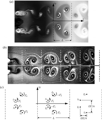
-function singularities of the vorticity field. Introduced by Helmholtz (Reference Helmholtz1858) in his seminal paper on vortex dynamics, this modelling framework conserves mass, interaction energy and discrete analogues of the linear and (possibly) angular momentum, referred to as the linear and angular impulse, and the analysis very often involves only a few degrees of freedom (see, e.g. Newton Reference Newton2001; Aref Reference Aref2007). The point-vortex approach can, hence, be considered as an idealized predictive tool for a broad range of real flows (Charney Reference Charney1963). The reader is referred to Meleshko & Aref (Reference Meleshko and Aref2007) for a detailed history of point-vortex modelling and applications. This mathematical framework has been used frequently to model wakes generated behind bluff bodies, a very common occurrence in nature. The vortical structures in a wake often assemble into a clearly identifiable persistent pattern, as illustrated in figure 1, with the details of the arrangement varying according to the number, circulation and relative positions of the vortices. Here we focus on the connection between point-vortex models and bluff body wakes, but this modelling approach is also applicable to similar vorticity distributions, such as that occurring with planar jets (Oler & Goldschmidt Reference Oler and Goldschmidt1982) or the Richtmyer–Meshkov instability of a gas curtain (Mikaelian Reference Mikaelian1996; Balakumar et al.
Reference Balakumar, Orlicz, Tomkins and Prestridge2008). The point-vortex approximation provides a significant resource for modelling the often-complex dynamics of these vorticity-dominated flows.
(a) A symmetric 2P wake generated by two stationary cylinders in a fluid moving left to right. Reproduced with permission from Fayed et al. (Reference Fayed, Portaro, Gunter, Abderrahmane and Ng2011); the image has been modified through a black/white inversion. Assumed vortex locations and circulation directions are marked in white. (b) A symmetric 2P wake generated by two rotating cylinders in a fluid moving left to right. Reproduced with permission from Kumar & Gonzalez (Reference Kumar and Gonzalez2010); see also Kumar, Gonzalez & Probst (Reference Kumar, Gonzalez and Probst2011b
). The wake snapshot has been rotated slightly (
 ${\approx}0.22^{\circ }$
clockwise) to maximize the locational symmetry of the vortices about the horizontal axis. White circles show the assumed vortex locations against which our model predictions are later compared (see § 5.2). (c) The singly periodic model arrangement of four point vortices in the complex plane.

The point-vortex approach to modelling wakes was first employed by von Kármán to represent the case in which two counter-rotating vortices are produced in each shedding period (von Kármán Reference von Kármán1911, Reference von Kármán1912; von Kármán & Rubach Reference von Kármán and Rubach1912). In this Kármán ‘vortex street’, as it is often called, the two rows of oppositely signed vortices align perpendicular to the mean flow and have an antisymmetric pattern with nearly constant horizontal and vertical spacing between successive vortices. Using the notation introduced by Williamson & Roshko (Reference Williamson and Roshko1988), this is the ‘2S’ wake, with the nomenclature signifying the presence of two ‘single’ vortices in each shedding period. In von Kármán’s point-vortex model, this wake is represented by two parallel, infinite rows of point vortices having equal and opposite circulations with exactly constant spacing between successive vortices. This system can also be viewed as a singly periodic array of two point vortices with opposite circulations, as first noted by Friedmann & Poloubarinova (Reference Friedmann and Poloubarinova1928). The assumption of spatial periodicity greatly simplifies the mathematical analysis while still giving an acceptable resemblance to the wakes observable naturally or in a laboratory environment.
Computational and mathematical investigations of bluff body wakes include point-vortex models with small numbers of vortices (see, e.g. von Kármán Reference von Kármán1911) or clouds of vortices (see, e.g. Sarpkaya & Schoaff Reference Sarpkaya and Schoaff1979), vortex panel methods (see, e.g. Hoeijmakers & Vaatstra Reference Hoeijmakers and Vaatstra1983) and direct numerical simulations in two dimensions (see, e.g. Silva, Silveira-Neto & Damasceno Reference Silva, Lima, Silveira-Neto and Damasceno2003) and in three dimensions (see, e.g. Ploumhans et al. Reference Ploumhans, Winckelmans, Salmon, Leonard and Warren2002). Much of the existing work has focused on understanding the mechanisms behind the vortex shedding and wake formation processes and on predicting the forces acting on the object. With the exception of the few low-order point-vortex models, computational investigations of the full wake dynamics are similar to the experimental investigations, in the sense that specific sets of parameters must be considered on a case-by-case basis. Such investigations can be quite formidable without guidance from a reduced-order theoretical analysis. Thus, in the spirit of von Kármán’s work, this point-vortex approach has been applied to investigating the relatively more ‘exotic’ wakes with three or more vortices generated during each shedding period (Aref, Stremler & Ponta Reference Aref, Stremler and Ponta2006; Stremler et al. Reference Stremler, Salmanzadeh, Basu and Williamson2011; Stremler & Basu Reference Stremler and Basu2014; Basu & Stremler Reference Basu and Stremler2015).
Point-vortex modelling of exotic wakes begins with considering a two-dimensional potential flow containing
 $N$
embedded ‘base’ point vortices having strengths
 $\unicode[STIX]{x1D6E4}_{\unicode[STIX]{x1D6FC}}$
,
 $\unicode[STIX]{x1D6FC}=1,\ldots ,N$
, at locations
 $z_{\unicode[STIX]{x1D6FC}}=x_{\unicode[STIX]{x1D6FC}}+\text{i}y_{\unicode[STIX]{x1D6FC}}$
,
 $\unicode[STIX]{x1D6FC}=1,\ldots ,N$
, on the complex plane, together with their periodic images at
 $z_{\unicode[STIX]{x1D6FC}}\pm nL$
,
 $n=1,\ldots ,\infty$
, with
 $L$
being the extent of the spatial period. An analogous consideration is that of
 $N$
vortices at
 $z_{\unicode[STIX]{x1D6FC}}$
in the strip
 $x\in [0,L]$
,
 $y\in (-\infty ,\infty )$
, with periodic boundary conditions imposed at
 $x=0,L$
. The relevant vortex dynamics is determined by solving the equations (Friedmann & Poloubarinova Reference Friedmann and Poloubarinova1928; Stremler Reference Stremler2010)
 $$\begin{eqnarray}\frac{\text{d}z_{\unicode[STIX]{x1D6FC}}^{\ast }}{\text{d}t}=\frac{1}{2L\text{i}}\sum _{\unicode[STIX]{x1D6FD}=1}^{N}\unicode[STIX]{x1D6E4}_{\unicode[STIX]{x1D6FD}}\cot \left[\frac{\unicode[STIX]{x03C0}}{L}(z_{\unicode[STIX]{x1D6FC}}-z_{\unicode[STIX]{x1D6FD}})\right],\end{eqnarray}$$
where the asterisk indicates complex conjugation and the prime on the summation signifies exclusion of the singular term
 $\unicode[STIX]{x1D6FC}=\unicode[STIX]{x1D6FD}$
. This point-vortex system can be represented as a Hamiltonian dynamical system having the form
 $$\begin{eqnarray}\unicode[STIX]{x1D6E4}_{\unicode[STIX]{x1D6FC}}\frac{\text{d}x_{\unicode[STIX]{x1D6FC}}}{\text{d}t}=\frac{\unicode[STIX]{x2202}H}{\unicode[STIX]{x2202}y_{\unicode[STIX]{x1D6FC}}},\quad \unicode[STIX]{x1D6E4}_{\unicode[STIX]{x1D6FC}}\frac{\text{d}y_{\unicode[STIX]{x1D6FC}}}{\text{d}t}=-\frac{\unicode[STIX]{x2202}H}{\unicode[STIX]{x2202}x_{\unicode[STIX]{x1D6FC}}},\end{eqnarray}$$
with the Hamiltonian
 $$\begin{eqnarray}H(z_{1},\ldots ,z_{N};\unicode[STIX]{x1D6E4}_{1},\ldots ,\unicode[STIX]{x1D6E4}_{N})=-\frac{1}{4\unicode[STIX]{x03C0}}\mathop{\sum }_{\unicode[STIX]{x1D6FC}=1}^{N}\sum _{\unicode[STIX]{x1D6FD}=1}^{N}\unicode[STIX]{x1D6E4}_{\unicode[STIX]{x1D6FC}}\unicode[STIX]{x1D6E4}_{\unicode[STIX]{x1D6FD}}\ln \left|\sin \left[\frac{\unicode[STIX]{x03C0}}{L}(z_{\unicode[STIX]{x1D6FC}}-z_{\unicode[STIX]{x1D6FD}})\right]\right|\end{eqnarray}$$
as a constant of motion. As on the infinite plane, the components of the linear impulse, namely
 $$\begin{eqnarray}Q+\text{i}P=\mathop{\sum }_{\unicode[STIX]{x1D6FC}=1}^{N}\unicode[STIX]{x1D6E4}_{\unicode[STIX]{x1D6FC}}z_{\unicode[STIX]{x1D6FC}},\end{eqnarray}$$
remain conserved (Birkhoff & Fisher Reference Birkhoff and Fisher1959) throughout the motion, since this periodic system is invariant with respect to translation. However, unlike on the infinite plane, the angular impulse is not preserved for this periodic system, as it is not invariant to rotation of the vortex configuration.
Since the individual vortex strengths remain unchanged over time in this inviscid model, the sum of the vortex strengths,
 $$\begin{eqnarray}S=\mathop{\sum }_{\unicode[STIX]{x1D6FC}=1}^{N}\unicode[STIX]{x1D6E4}_{\unicode[STIX]{x1D6FC}},\end{eqnarray}$$
is also a constant of the motion. The modelling framework is motivated by periodic symmetric shedding from a bluff body, and hence we will further assume that
 $S=0$
.
A full classification of the spatially periodic point-vortex motion for
 $N=3$
and
 $S=0$
has been provided by Aref & Stremler (Reference Aref and Stremler1996). Equations (1.3)–(1.5) (with
 $S=0$
) provide sufficient constraints that this three-vortex system is integrable. The comparison by Aref & Stremler (Reference Aref and Stremler1996) to the three-dimensional experimental wakes of Williamson & Roshko (Reference Williamson and Roshko1988), revisited in a more recent study by Stremler & Basu (Reference Stremler and Basu2014), demonstrates that the point-vortex model is capable of giving a reasonable representation of the vortex motion in a ‘P+S’ wake, in which three vortices (one ‘pair’ and one ‘single’) are shed in each period. This remarkable similarity between the experimental vortex motion and the temporal evolution of the point-vortex system, produced as described in § 5.2, helps motivate the current work.
Exploring the
 $N=4$
case as a suitable model for 2P wakes, in which four vortices (i.e. two ‘pairs’) are generated in each shedding cycle, has been the next avenue of study. The 2P wake is the most commonly observed pattern amongst the exotic vortex wakes (Williamson & Govardhan Reference Williamson and Govardhan2004). In contrast to the
 $N=3$
case, there are not sufficient constants of motion for the general four-vortex system to be integrable. This lack of integrability is true even when the motion is considered on the unbounded plane, where the angular impulse is an added constant of motion (Aref & Pomphrey Reference Aref and Pomphrey1982; Aref & Stremler Reference Aref and Stremler1999). However, we have established (Stremler et al.
Reference Stremler, Salmanzadeh, Basu and Williamson2011; Stremler & Basu Reference Stremler and Basu2014) that the periodic
 $N=4$
case can indeed be transformed into an integrable Hamiltonian system by assuming that the base vortex circulations and positions are related according to
 $$\begin{eqnarray}\left.\begin{array}{@{}c@{}}\displaystyle \unicode[STIX]{x1D6E4}_{3}=-\unicode[STIX]{x1D6E4}_{1},\quad z_{3}=z_{1}^{\ast }-d\equiv \unicode[STIX]{x1D701}_{1},\\ \displaystyle \unicode[STIX]{x1D6E4}_{4}=-\unicode[STIX]{x1D6E4}_{2},\quad z_{4}=z_{2}^{\ast }+d\equiv \unicode[STIX]{x1D701}_{2},\end{array}\right\}\end{eqnarray}$$
where
 $d$
is real valued and constant and the asterisk again denotes complex conjugation. We use
 $\unicode[STIX]{x1D701}_{i}$
(
 $i=1,2$
) to represent the positions of the constrained vortices. This symmetry, inspired by the vortex arrangements observed in experimental wakes, is preserved by the equations of motion (1.1) provided
 $$\begin{eqnarray}d=mL/2,\quad m=0,1.\end{eqnarray}$$
The choice
 $m=1$
corresponds to a glide-reflective symmetry, in which there is a half-period shift between the reflected vortex pairs; this case has been addressed fully by Basu & Stremler (Reference Basu and Stremler2015). For completeness, in this section we reproduce relevant aspects of the mathematical derivation given earlier in Basu (Reference Basu2014), Stremler & Basu (Reference Stremler and Basu2014) and Basu & Stremler (Reference Basu and Stremler2015).
In the present treatment, we focus on the reflectively symmetric configuration with
 $m=0$
. Figure 1(a,b) depicts examples of the related symmetric 2P wakes observed in the laboratory. The two pairs generated in each shedding cycle are mirror images of each other about the wake centreline. In the
 $N=4$
singly periodic point-vortex system constrained by (1.6a
), this symmetry corresponds to
 $d=0$
, giving
 $$\begin{eqnarray}\unicode[STIX]{x1D701}_{1}=z_{1}^{\ast },\quad \unicode[STIX]{x1D701}_{2}=z_{2}^{\ast }.\end{eqnarray}$$
The strength of the vortex at
 $\unicode[STIX]{x1D701}_{1}$
is
 $-\unicode[STIX]{x1D6E4}_{1}$
, and the strength of the vortex at
 $\unicode[STIX]{x1D701}_{2}$
is
 $-\unicode[STIX]{x1D6E4}_{2}$
. Figure 1(c) illustrates the spatial symmetry assumptions for this four-vortex system.
The geometric constraint (1.6) on the vortex dynamics enables us to keep track of the motion of all four base vortices in terms of just the separation between the vortices at
 $z_{1}$
and
 $z_{2}$
, which we write in non-dimensional form as
 $$\begin{eqnarray}Z=X+\text{i}Y=\unicode[STIX]{x03C0}(z_{1}-z_{2})/L.\end{eqnarray}$$
To assist with non-dimensionalization, we also introduce the quantities
 $$\begin{eqnarray}\mathbb{S}=\unicode[STIX]{x1D6E4}_{1}+\unicode[STIX]{x1D6E4}_{2},\quad \unicode[STIX]{x1D6FE}=\unicode[STIX]{x1D6E4}_{1}/\mathbb{S}.\end{eqnarray}$$
Note that we can assume
 $0\leqslant \unicode[STIX]{x1D6E4}_{1}\leqslant \unicode[STIX]{x1D6E4}_{2}$
without any loss of generality, and hence
 $\unicode[STIX]{x1D6FE}\in [0,1/2]$
covers all possible vortex strength combinations.
Under the constraint (1.6), the components of the linear impulse (1.4) are given by
 $$\begin{eqnarray}Q=d(\unicode[STIX]{x1D6E4}_{1}-\unicode[STIX]{x1D6E4}_{2})=0,\quad P=2(\unicode[STIX]{x1D6E4}_{1}y_{1}+\unicode[STIX]{x1D6E4}_{2}y_{2}),\end{eqnarray}$$
which can be written in non-dimensional form as
 $$\begin{eqnarray}{\mathcal{Q}}=\frac{\unicode[STIX]{x03C0}}{L\mathbb{S}}Q=0,\quad {\mathcal{P}}=\frac{\unicode[STIX]{x03C0}}{L\mathbb{S}}P=\frac{2\unicode[STIX]{x03C0}}{L}[\unicode[STIX]{x1D6FE}y_{1}+(1-\unicode[STIX]{x1D6FE})y_{2}].\end{eqnarray}$$
Coupling these representations of the linear impulse with (1.7) leads us to
 $$\begin{eqnarray}y_{1}=\frac{L}{\unicode[STIX]{x03C0}}\left[\frac{{\mathcal{P}}}{2}+(1-\unicode[STIX]{x1D6FE})Y\right],\quad y_{2}=\frac{L}{\unicode[STIX]{x03C0}}\left[\frac{{\mathcal{P}}}{2}-\unicode[STIX]{x1D6FE}Y\right].\end{eqnarray}$$
For
 $\unicode[STIX]{x1D6FE}\neq 0$
, substitution of (1.6), (1.7), and (1.10) into (1.3), together with the rescaling
 $$\begin{eqnarray}{\mathcal{H}}=\frac{H}{\mathbb{S}^{2}\unicode[STIX]{x1D6FE}(1-\unicode[STIX]{x1D6FE})},\end{eqnarray}$$
enables the Hamiltonian for these symmetric four-vortex configurations in a period strip to be written as (cf. (12) in Basu & Stremler (Reference Basu and Stremler2015))
 $$\begin{eqnarray}\displaystyle {\mathcal{H}}(Z;\unicode[STIX]{x1D6FE},{\mathcal{P}}) & = & \displaystyle -\frac{1}{2\unicode[STIX]{x03C0}}\left[\ln \left|\frac{\sin ^{2}X+\sinh ^{2}Y}{\sin ^{2}X+\sinh ^{2}[{\mathcal{P}}+(1-2\unicode[STIX]{x1D6FE})Y]}\right|\right.\nonumber\\ \displaystyle & & \displaystyle \left.-\,\frac{\unicode[STIX]{x1D6FE}}{1-\unicode[STIX]{x1D6FE}}\ln |\sinh [{\mathcal{P}}+2(1-\unicode[STIX]{x1D6FE})Y]|-\frac{1-\unicode[STIX]{x1D6FE}}{\unicode[STIX]{x1D6FE}}\ln |\sinh [{\mathcal{P}}-2\unicode[STIX]{x1D6FE}Y]|\right].\nonumber\\ \displaystyle & & \displaystyle\end{eqnarray}$$
For
 $\unicode[STIX]{x1D6FE}=0$
, the Hamiltonian (1.3) reduces trivially to
 $$\begin{eqnarray}H=\frac{\unicode[STIX]{x1D6E4}_{2}^{2}}{2\unicode[STIX]{x03C0}}\ln |\sinh [{\mathcal{P}}]|,\end{eqnarray}$$
and we must treat this choice of
 $\unicode[STIX]{x1D6FE}$
as a special case, which we address in § 3.1.
By introducing the dimensionless time variable
 $$\begin{eqnarray}\unicode[STIX]{x1D70F}=\frac{\unicode[STIX]{x03C0}^{2}\mathbb{S}}{2L^{2}}t,\end{eqnarray}$$
the relative motion of vortices
 $z_{1}$
and
 $z_{2}$
, as given by the evolution of
 $(X,Y)$
, can be written in canonical form as
 $$\begin{eqnarray}\frac{\text{d}X}{\text{d}\unicode[STIX]{x1D70F}}=\frac{\unicode[STIX]{x2202}{\mathcal{H}}}{\unicode[STIX]{x2202}Y},\quad \frac{\text{d}Y}{\text{d}\unicode[STIX]{x1D70F}}=-\frac{\unicode[STIX]{x2202}{\mathcal{H}}}{\unicode[STIX]{x2202}X}.\end{eqnarray}$$
This reduction to a two-degree-of-freedom dynamical system, with parametric dependence on
 $(\unicode[STIX]{x1D6FE},{\mathcal{P}})$
, shows that the relative vortex motion is integrable.
Numerical integration of the system in (1.15) for a particular choice of
 $(\unicode[STIX]{x1D6FE},{\mathcal{P}})$
gives the relative vortex motion as it follows a particular level curve in the
 $(X,Y)$
phase plane, with that curve determined by the initial relative position of
 $z_{1}$
and
 $z_{2}$
. The corresponding motion of the four-vortex system in a frame of reference with zero background flow can then be determined by numerical integration of any one of equations (1.1) subject to the constraint that
 ${\mathcal{H}}$
is constant.
The remainder of the manuscript consists of the following. The details of a representative example of the possible point-vortex motions for one specific choice of
 $\unicode[STIX]{x1D6FE}$
and
 ${\mathcal{P}}$
are given in § 2. The special cases produced by choosing
 $\unicode[STIX]{x1D6FE}=0$
or
 $\unicode[STIX]{x1D6FE}=1/2$
are addressed in § 3. Characterization of bifurcations in the topology of the phase space structure is given in § 4. In § 5.1, we examine in some detail the neutrally stable relative equilibria that can appear for sufficiently large values of
 $|{\mathcal{P}}|$
and consider how that characterization can be applied to experimental wakes such as that shown in figure 1(a). This is followed in § 5.2 by a comparison of the dynamically evolving model trajectories to the experimental wake in figure 1(b). We conclude in § 6.
A preliminary report on this work was presented at the annual meeting of the APS Division of Fluid Dynamics in Pittsburgh, PA, November 2013 (Basu & Stremler Reference Basu and Stremler2013). Preliminary results were first published in the thesis of Basu (Reference Basu2014).
2 A representative example:
 $\unicode[STIX]{x1D6FE}=3/7$
,
${\mathcal{P}}=-1$


The symmetric vortex system is analysed here by first exploring a representative example with
 $\unicode[STIX]{x1D6FE}=3/7$
, which correlates to the vortex strength ratio
 $\unicode[STIX]{x1D6E4}_{1}:\unicode[STIX]{x1D6E4}_{2}=3:4$
and
 ${\mathcal{P}}=-1$
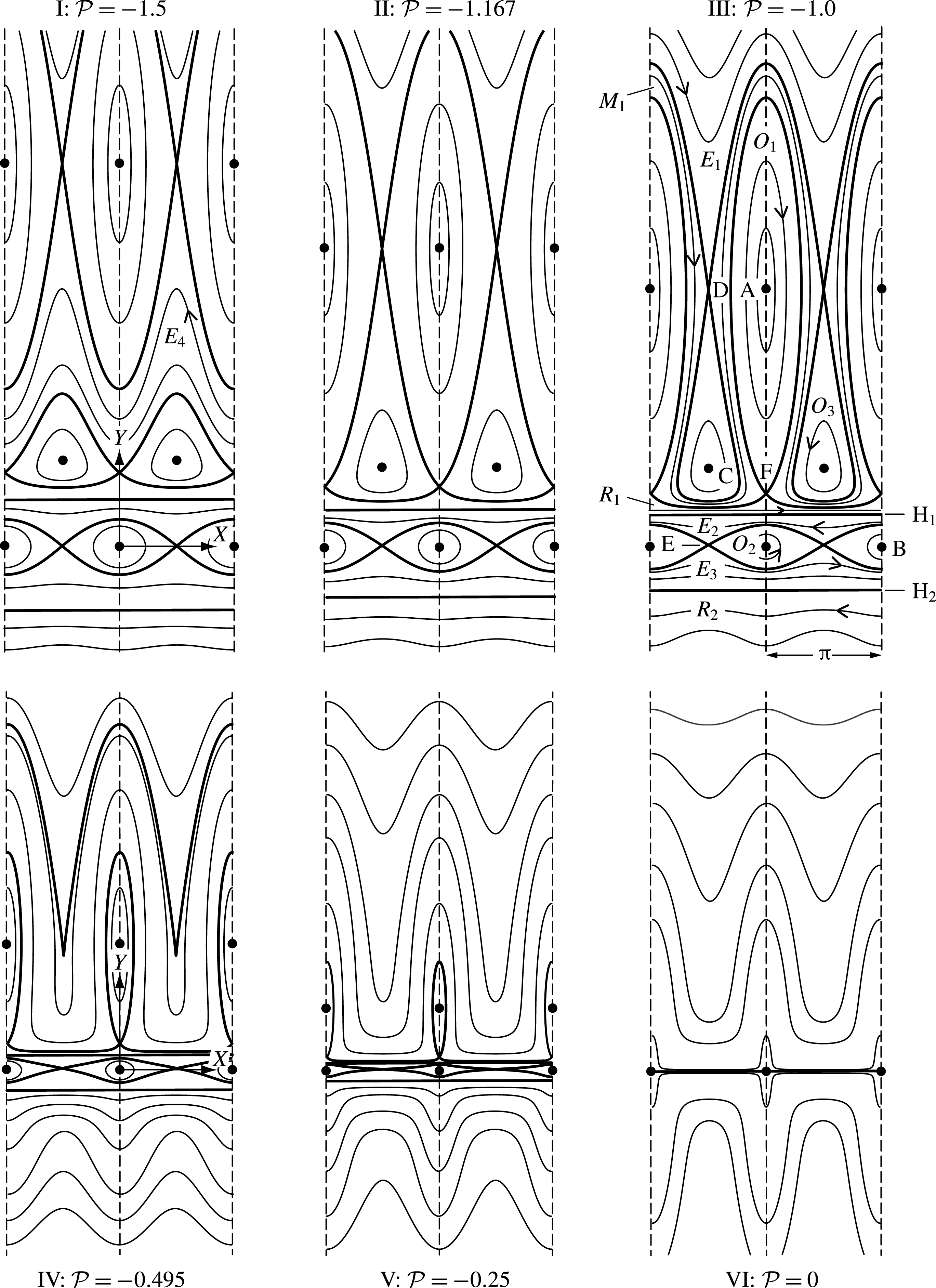
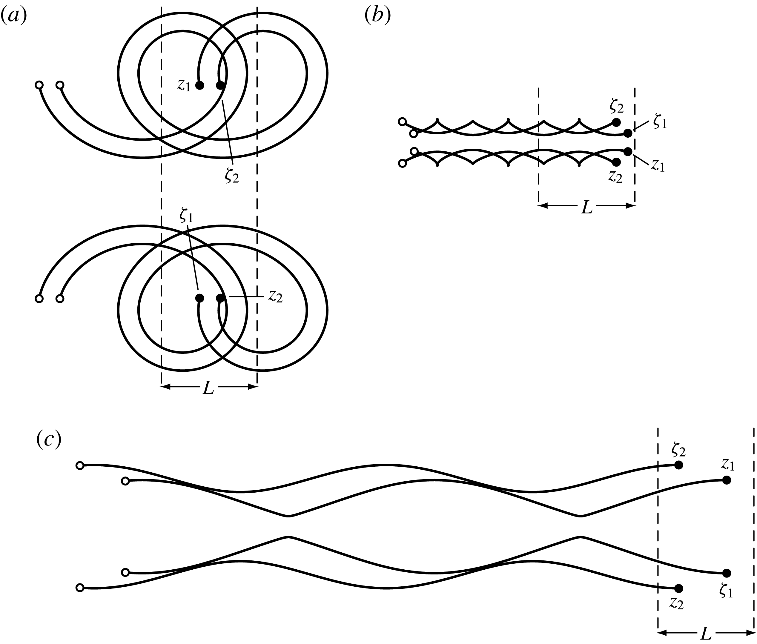
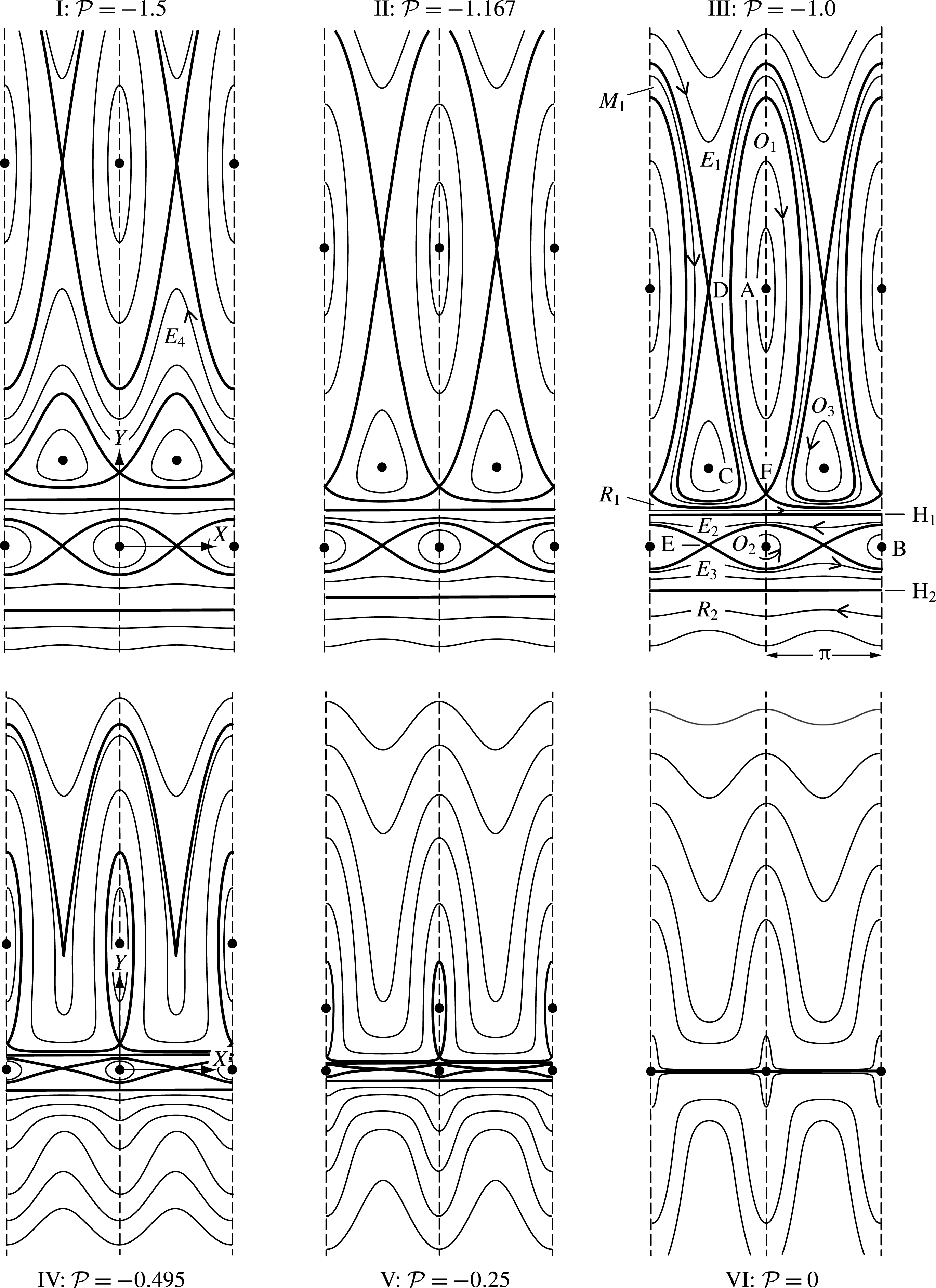
. Panel III of figure 2 shows the representative phase space trajectories for this selection of the parameters. Along each trajectory in the
 $(X,Y)$
phase space, the Hamiltonian
 ${\mathcal{H}}(X,Y;\unicode[STIX]{x1D6FE},{\mathcal{P}})$
in (1.11) remains constant, and the different trajectories correspond to different values of this conserved quantity. Each period of the phase domain contains six fixed points, representing relative equilibria of the vortex configurations; these relative equilibria are discussed in § 2.1. Singularities in the Hamiltonian occur along the lines marked H
 $_{1}$
and H
 $_{2}$
, as discussed in § 2.2. These horizontal lines and the level curves passing through the saddle fixed points (or separatrices) divide the phase space into nine distinct regimes of motion. In each such regime, the relative vortex dynamics has the same qualitative characteristics irrespective of the exact initial conditions. The vortex motion within each of these regimes, which are labelled
 $O_{i}$
,
 $E_{i}$
,
 $R_{i}$
and
 $M_{1}$
in panels I and III of figure 2, is described in § 2.4.
Representative level curves of
 ${\mathcal{H}}$
in the
 $(X,Y)$
plane for
 $\unicode[STIX]{x1D6FE}=3/7$
and various values of
 $|{\mathcal{P}}|$
. Heavy lines show separatrices and the
 $\text{H}_{i}$
(
 $i=1,2$
) lines. Circles show elliptic fixed points and saddle fixed points are located at the intersections of separatrices; fixed points are labelled A–F. Panels are labelled by Roman numerals I–VI and the corresponding values of
 ${\mathcal{P}}$
. In panel III, the different distinct regimes of motion are labelled
 $O_{i}$
,
 $E_{i}$
,
 $R_{i}$
or
 $M_{1}$
based on the corresponding type of vortex motion; regime
 $E_{4}$
, which does not appear in panel III, is labelled in panel I. Arrows on level curves indicate the direction of phase trajectory evolution. Panels II, IV and VI show (approximately) bifurcation points in the phase space topology. Each panel shows two spatial periods for clarity.
 $X$
and
 $Y$
axes are all shown to the same scale.
The mathematical structure in (1.12) confirms that
 ${\mathcal{H}}$
stays invariant under the transformation
 $\{Y\rightarrow -Y,~{\mathcal{P}}\rightarrow -{\mathcal{P}}\}$
. Topologically, this invariance implies that changing the sign of
 ${\mathcal{P}}$
corresponds to a reflection of the phase trajectories about the
 $X$
-axis. Changing the sign of
 ${\mathcal{P}}$
changes the signs of the vortex circulations, which reverses the direction of motion along the phase trajectories and the direction of the real space vortex motion. Examples of experimental symmetric 2P wakes in the published literature (see figure 1) and examples communicated privately by a colleague (W. Yang, Virginia Tech, private communication) correspond primarily to orientations with negative values of
 ${\mathcal{P}}$
. Thus, without any loss of generality, we have assumed
 ${\mathcal{P}}<0$
for our analysis.
2.1 Vortex configurations in relative equilibrium
The points labelled A–F in panel III of figure 2, together with their periodic images, correspond to relative equilibrium vortex configurations, wherein the vortices propagate along the
 $x$
axis without change in their relative positions. Of these, A–C are elliptic fixed points (or centres), corresponding to vortex configurations that are neutrally stable to infinitesimal perturbations in the
 $Z$
-plane. Thus, for these cases a perturbation in the
 $Z$
-plane that does not otherwise change the vortex strengths, the linear impulse and the assumed geometry generates an orbiting phase trajectory close to the corresponding fixed point. The value of the Hamiltonian is necessarily changed by this perturbation, but
 ${\mathcal{H}}$
remains conserved in the perturbed system. The points D–F are saddle fixed points, corresponding to relative equilibrium vortex arrangements that are unstable to infinitesimal perturbations in
 $Z$
. These perturbed configurations can deviate widely from the initial unperturbed vortex arrangement and typically involve a change in
 ${\mathcal{H}}$
. However, if the perturbation is such that the new
 $(X,Y)$
coordinates lie on the separatrix passing through the saddle point, then the value of the Hamiltonian is conserved by the perturbation. In such cases, the perturbed vortex configuration will approach a relative equilibrium configuration, which may be a different configuration than the original.
Relative equilibrium vortex configurations and representative streamlines in the appropriate co-moving reference frame on the
 $(x,y)$
-plane for
 $\unicode[STIX]{x1D6FE}=3/7$
and
 ${\mathcal{P}}=-1$
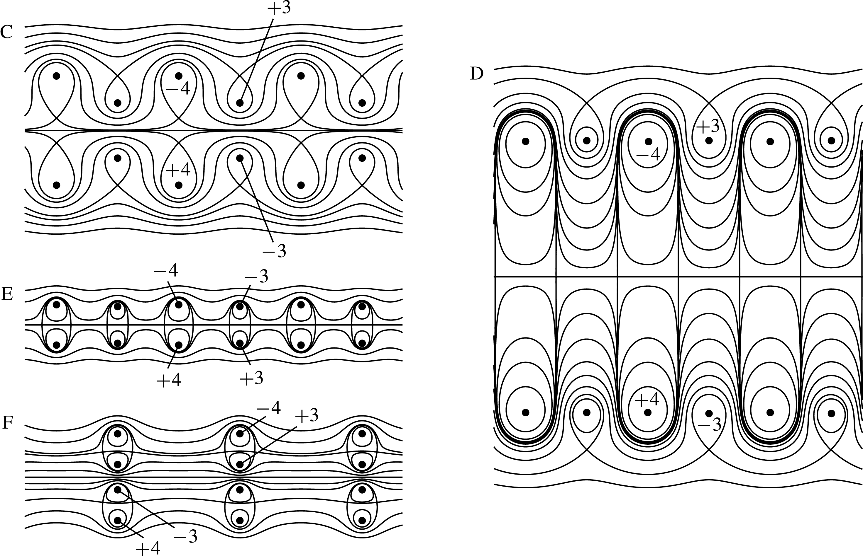
; the corresponding phase plane representation is shown in panel III of figure 2. Panels are labelled according to the corresponding fixed point on the phase plane. Representative vortices are labelled according to their strength. Each of these relative equilibrium configurations translates steadily to the left with respect to a fixed frame and without change in shape or orientation. The
 $x$
and
 $y$
axes are all shown to the same scale.

Consider the point labelled A in panel III of figure 2, for which
 $X=n\unicode[STIX]{x03C0}$
(with
 $n$
any integer) and
 $Y>0$
. This point corresponds to the singularity in
 ${\mathcal{H}}$
that occurs when the oppositely signed vortices coincide, leaving two widely spaced symmetrically reflective rows of oppositely signed vortices, or only two base vortices in each periodic strip, with strengths
 $\pm (\unicode[STIX]{x1D6E4}_{1}-\unicode[STIX]{x1D6E4}_{2})$
. Coincidence of the oppositely signed vortices is given by
 $z_{1}={z_{2}}^{\ast }\pm nL$
or
 $y_{1}=-y_{2}$
, and we find from (1.10) that
 $Y=-{\mathcal{P}}/(1-2\unicode[STIX]{x1D6FE})$
for this two-vortex relative equilibrium configuration.
Point B is also a singular case, with
 $X=n\unicode[STIX]{x03C0}$
(with
 $n$
any integer) and
 $Y=0$
, giving
 $z_{1}=z_{2}\pm nL$
. In this case the like-signed vortices coincide, and the relative equilibrium configuration consists of two rows of oppositely signed vortices having strengths
 $\pm (\unicode[STIX]{x1D6E4}_{1}+\unicode[STIX]{x1D6E4}_{2})$
.
Point C is one of three fixed points for which
 $X=(2n+1)\unicode[STIX]{x03C0}/2$
and
 $Y>0$
. As with points A and B, point C is a neutrally stable elliptic fixed point. In contrast to A and B, point C is not located at a singularity in
 ${\mathcal{H}}$
, and the corresponding vortex configuration consists of four distinct base vortices in each periodic strip, as illustrated in panel C of figure 3. This fixed point is unique, giving the only equilibrium state that is neutrally stable to perturbations on the
 $Z$
-plane while still preserving the four-vortex configuration. The value of
 $Y$
is found numerically by simultaneously solving
 $\unicode[STIX]{x2202}{\mathcal{H}}/\unicode[STIX]{x2202}Y=0$
and
 $\unicode[STIX]{x2202}{\mathcal{H}}/\unicode[STIX]{x2202}X=0$
. We consider these interesting relative equilibrium configurations in further detail in § 2.3 and § 5.1. A perturbation of these configurations that consists of varying
 $(X,Y)$
while maintaining the spatial symmetry and the values of
 $\unicode[STIX]{x1D6FE}$
and
 ${\mathcal{P}}$
leads to periodic relative vortex motion in the
 $O_{3}$
regime, as discussed in § 2.4.1.
Point D is a saddle point with
 $X=(2n+1)\unicode[STIX]{x03C0}/2$
and
 $Y>0$
. The value of
 $Y$
is obtained numerically using the same procedure as for point C. Panel D of figure 3 shows this relative equilibrium configuration, which consists of four base vortices per period with a relatively large vertical separation between the vortex pairs. In contrast to point C, the configuration for point D is unstable to perturbations in the
 $Z$
-plane.
Point E is the saddle point for which
 $X=(2n+1)\unicode[STIX]{x03C0}/2$
and
 $Y$
is small but finite, as determined numerically. Panel E of figure 3 shows this configuration with four separate base vortices and a very small vertical offset between the vortex pairs. While still satisfying the assumed arrangement illustrated in figure 1(b), the small vertical offset produces a configuration in which the primary pairing is between vortices of equal (and opposite) strength that are aligned vertically and centred on the
 $x$
axis. Since point E is a saddle point, this configuration is unstable to perturbations in the
 $Z$
-plane.
Point F is located at
 $X=n\unicode[STIX]{x03C0}$
and
 $Y>0$
, with the value of
 $Y$
again being obtained numerically. This saddle point corresponds to the relative equilibrium configuration shown in panel F of figure 3, in which the four base vortices (per period) are all aligned vertically. This case is the only four-vortex relative equilibrium configuration with
 $X=n\unicode[STIX]{x03C0}$
. This configuration is also unstable to
 $Z$
-plane perturbations.
2.2 Lines of singularity
In addition to the separatrices joining equilibrium points, there are two horizontal lines marked as H
 $_{1}$
and H
 $_{2}$
in panel III of figure 2 that also delineate phase space behaviour. These horizontal lines correspond to the singularities that occur in
 ${\mathcal{H}}$
when the image vortices, namely
 $\{z_{1},\unicode[STIX]{x1D701}_{1}\}$
or
 $\{z_{2},\unicode[STIX]{x1D701}_{2}\}$
, coincide. Along H
 $_{1}$
, we have
 $z_{1}=\unicode[STIX]{x1D701}_{1}$
, so that
 $y_{1}=0$
. Thus, by (1.10), the line for H
 $_{1}$
occurs at
 $Y={\mathcal{P}}/[2(\unicode[STIX]{x1D6FE}-1)]$
. The corresponding vortex arrangement comprises two rows of oppositely signed vortices with circulations
 $\pm \unicode[STIX]{x1D6E4}_{2}$
that are vertically aligned. Similarly, along H
 $_{2}$
the vortices at
 $z_{2}$
and
 $\unicode[STIX]{x1D701}_{2}$
coincide, so that
 $y_{2}=0$
, which by (1.10) gives the location of H
 $_{2}$
as
 $Y={\mathcal{P}}/(2\unicode[STIX]{x1D6FE})$
. The corresponding vortex configuration consists of two rows of oppositely signed, symmetrically aligned vortices with circulations
 $\pm \unicode[STIX]{x1D6E4}_{1}$
. As
 $|{\mathcal{P}}|\rightarrow 0$
, both lines of singularity merge asymptotically with the
 $X$
axis. Note that these two horizontal lines of singularity in the phase plane do not appear in the staggered configuration we examine in Basu & Stremler (Reference Basu and Stremler2015).
2.3 A note on the stability of relative equilibria
Elsewhere in this manuscript, stability of relative equilibrium configurations is considered within the context of the assumed system constraints. That is, configurations A–C are shown, through reference to phase space diagrams such as those in figure 2, to be neutrally stable to small perturbations in the vortex locations that preserve the vortex strengths, the value of the linear impulse (1.9), and the symmetry in the relative vortex positions given by (1.6). Within this context, perturbations need not be infinitesimal. However, the significance of this (nonlinear) stability is limited by its reliance on preserving the spatial symmetry.
One can ask whether the unique configurations corresponding to point C are stable to perturbations that break the spatial symmetry. Through a number of numerical experiments, we have determined that these configurations do indeed appear to be stable to arbitrary, small perturbations that preserve the vortex strengths, the linear impulse and the
 $L$
-periodicity of the system. The effects of longer wavelength perturbations remain to be determined.
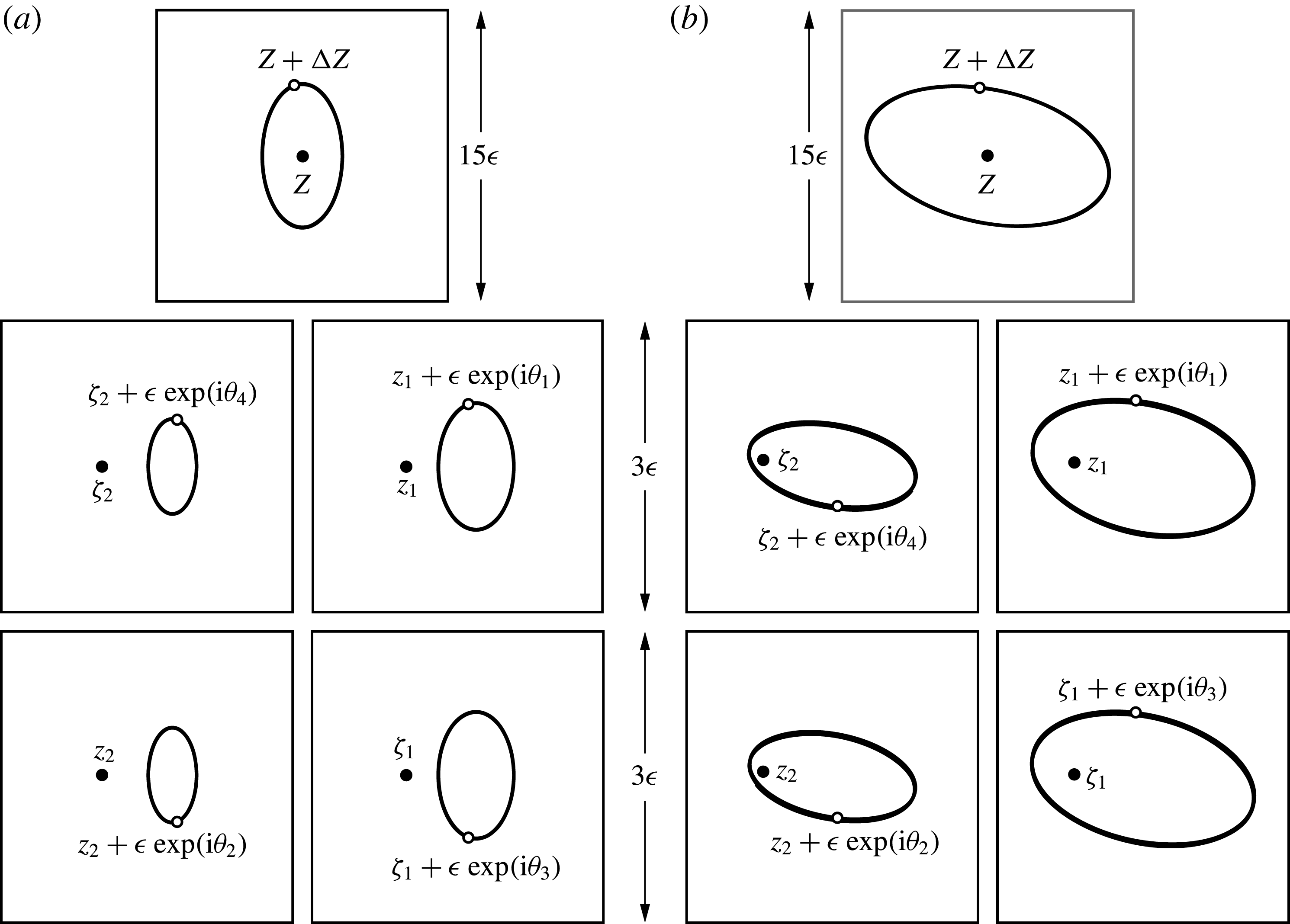
Dynamics of the system perturbed from the equilibrium configuration in panel C of figure 3 for
 $\unicode[STIX]{x1D6FE}=3/7$
and
 ${\mathcal{P}}=-1$
using
 $\unicode[STIX]{x1D716}=L/1000$
,
 $\unicode[STIX]{x1D703}_{1}=\unicode[STIX]{x03C0}/4$
and
 $\unicode[STIX]{x1D703}_{2}=\sin ^{-1}[-\unicode[STIX]{x1D6E4}_{1}(\sin \unicode[STIX]{x1D703}_{1})/\unicode[STIX]{x1D6E4}_{2}]\approx -0.559$
: (a) shows the symmetric case with
 $\unicode[STIX]{x1D703}_{3}=-\unicode[STIX]{x1D703}_{1}$
,
 $\unicode[STIX]{x1D703}_{4}=-\unicode[STIX]{x1D703}_{2}$
; (b) shows the other solution to (2.2a
),
 $\unicode[STIX]{x1D703}_{3}=\unicode[STIX]{x1D703}_{1}$
,
 $\unicode[STIX]{x1D703}_{4}=\unicode[STIX]{x1D703}_{2}$
, which breaks the spatial symmetry. Panels in the topmost row show phase plane trajectories for the initial condition
 $Z+\unicode[STIX]{x0394}Z=\unicode[STIX]{x03C0}[(z_{1}-z_{2})+\unicode[STIX]{x1D716}(\text{e}^{i\unicode[STIX]{x1D703}_{1}}-\text{e}^{i\unicode[STIX]{x1D703}_{2}})]/L$
; the unperturbed
 $Z$
is shown for reference. Panels in the bottom two rows show close-up views of the trajectories of the perturbed vortices in a frame of reference moving with the vortices in the equilibrium configuration, positions of which are also shown for reference. Integration time for both cases is
 $\unicode[STIX]{x0394}\unicode[STIX]{x1D70F}=500$
. Calculations were performed using
 $L=\mathbb{S}=1$
.

In the numerical experiments, vortices in an equilibrium configuration with locations
 $z_{\unicode[STIX]{x1D6FC}}$
,
 $\unicode[STIX]{x1D701}_{\unicode[STIX]{x1D6FC}}$
were given perturbations of the form
 $$\begin{eqnarray}\left.\begin{array}{@{}c@{}}\hat{z}_{1}=z_{1}+\unicode[STIX]{x1D716}\exp (\text{i}\unicode[STIX]{x1D703}_{1}),\quad \hat{z}_{2}=z_{2}+\unicode[STIX]{x1D716}\exp (\text{i}\unicode[STIX]{x1D703}_{2}),\\ \hat{\unicode[STIX]{x1D701}}_{1}=\unicode[STIX]{x1D701}_{1}+\unicode[STIX]{x1D716}\exp (\text{i}\unicode[STIX]{x1D703}_{3}),\quad \hat{\unicode[STIX]{x1D701}}_{2}=\unicode[STIX]{x1D701}_{2}+\unicode[STIX]{x1D716}\exp (\text{i}\unicode[STIX]{x1D703}_{4}),\end{array}\right\}\end{eqnarray}$$
where the magnitude of the perturbation,
 $\unicode[STIX]{x1D716}$
, was assumed to be the same for each vortex. These perturbed positions were used as initial conditions in the equations of motion (1.1), which were integrated in time using Wolfram Mathematica™. Applying a perturbation that preserves the linear impulse (1.4) requires that the perturbation angles be related according to
 $$\begin{eqnarray}\displaystyle & \displaystyle \unicode[STIX]{x1D6E4}_{1}(\cos \unicode[STIX]{x1D703}_{1}-\cos \unicode[STIX]{x1D703}_{3})=-\unicode[STIX]{x1D6E4}_{2}(\cos \unicode[STIX]{x1D703}_{2}-\cos \unicode[STIX]{x1D703}_{4}), & \displaystyle\end{eqnarray}$$
 $$\begin{eqnarray}\displaystyle & \displaystyle \unicode[STIX]{x1D6E4}_{1}(\sin \unicode[STIX]{x1D703}_{1}-\sin \unicode[STIX]{x1D703}_{3})=-\unicode[STIX]{x1D6E4}_{2}(\sin \unicode[STIX]{x1D703}_{2}-\sin \unicode[STIX]{x1D703}_{4}). & \displaystyle\end{eqnarray}$$
 $\unicode[STIX]{x1D703}_{3}=-\unicode[STIX]{x1D703}_{1}$
and
 $\unicode[STIX]{x1D703}_{4}=-\unicode[STIX]{x1D703}_{2}$
, so that (2.2a
) is satisfied automatically and (2.2b
) becomes
 $$\begin{eqnarray}\unicode[STIX]{x1D6E4}_{1}\sin \unicode[STIX]{x1D703}_{1}=-\unicode[STIX]{x1D6E4}_{2}\sin \unicode[STIX]{x1D703}_{2}.\end{eqnarray}$$
In figure 4 we show two representative examples of the dynamics that occurs when the equilibrium configuration from panel C of figure 3 is perturbed according to (2.1) and (2.2). For the sake of comparison, these examples were chosen to have the same perturbed value of
 $Z$
. The example in figure 4(a) preserves the spatial symmetry, and thus is clearly (neutrally) stable according to the analysis presented in the remainder of this manuscript. The example in figure 4(b) breaks this symmetry and yet still shows similar results, indicating that the system remains neutrally stable under (small) arbitrary perturbations that satisfy (2.2). All other perturbation choices that were tested produced similar behaviour (not shown). We evaluated the accuracy of the numerical solutions by monitoring variations in the time-dependent values of what should be constants of the motion, as given by
 $$\begin{eqnarray}{\mathcal{E}}_{{\mathcal{Q}}}(t)=\left|\frac{{\mathcal{Q}}(t)-{\mathcal{Q}}(0)}{{\mathcal{Q}}(0)}\right|,\quad {\mathcal{E}}_{{\mathcal{P}}}(t)=\left|\frac{{\mathcal{P}}(t)-{\mathcal{P}}(0)}{{\mathcal{P}}(0)}\right|,\quad {\mathcal{E}}_{{\mathcal{H}}}(t)=\left|\frac{{\mathcal{H}}(t)-{\mathcal{H}}(0)}{{\mathcal{H}}(0)}\right|.\end{eqnarray}$$
For the cases shown in figure 4, an integration time of
 $\unicode[STIX]{x0394}\unicode[STIX]{x1D70F}=500$
gives
 ${\mathcal{E}}_{{\mathcal{Q}}}<10^{-14}$
,
 ${\mathcal{E}}_{{\mathcal{P}}}<10^{-15}$
and
 ${\mathcal{E}}_{{\mathcal{H}}}<10^{-6}$
for all
 $0\leqslant \unicode[STIX]{x1D70F}\leqslant 500$
. During this integration time, the vortex configurations travel a distance greater than
 $21L$
along the
 $x$
axis.
2.4 Vortex motions for
$\unicode[STIX]{x1D6FE}=3/7$
,
${\mathcal{P}}=-1$


As outlined in § 1, the motion of the four base vortices (and their periodic images) in the
 $(x,y)$
plane is given by the relative vortex motion along a level curve in panel III of figure 2, together with constrained integration of one equation from (1.1). Vortex motion within each regime of motion is qualitatively the same, and thus we can explore all possible motions for
 $(\unicode[STIX]{x1D6FE},{\mathcal{P}})=(3/7,-1)$
by considering one example trajectory from each regime. These nine regimes of motion can be classified as giving four different general types of vortex motion, which we refer to as orbiting motion, exchanging motion, reverse exchanging motion and mixed motion.
2.4.1 Orbiting motion
We begin by focusing on the regions in phase space around each of the elliptic points A, B and C. As shown for the representative example in panel III of figure 2, we label these regimes as
 $O_{i}$
, with the index
 $i$
being 1, 2 or 3 according to if the regime is located around point A, B or C, respectively. These regions are bounded by separatrices passing through the neighbouring saddle points (points D and F for
 $O_{1}$
and
 $O_{3}$
; point E for
 $O_{2}$
). As a result, the relative separations of the vortices remain bounded for all time. When the initial conditions lie in any one of these regions, the corresponding vortex separation,
 $Z$
, orbits periodically about the fixed point on an elliptical phase trajectory. Hence, we refer to these regimes as orbiting regimes. Examples of physical space vortex motion from the
 $O_{i}$
regimes are shown in figure 5. Since the relative separation
 $Z$
is periodic in time, the initial vortex arrangement is repeated periodically in time, although in general there will also be a net translation of the entire configuration.
Representative examples of orbiting motion for
 $(\unicode[STIX]{x1D6FE},{\mathcal{P}})=(3/7,-1)$
in the singly periodic
 $(x,y)$
-plane with period
 $L$
. Initial conditions belong to the regimes (a)
 $O_{1}$
, (b)
 $O_{2}$
and (c)
 $O_{3}$
, respectively, corresponding to the regimes labelled in panel III of figure 2. Solid circles mark initial vortex locations, labelled according to the vortex definitions in figure 1. Solid lines trace out pathlines of the vortices for (a,c) two and for (b) three periods of the relative vortex motion. Open circles mark the reconstituted vortex configurations. The
 $x$
and
 $y$
axes are all shown to the same scale.

In regime
 $O_{1}$
, the vortex separation
 $Z$
orbits periodically in a clockwise sense along a closed elliptical trajectory around point A in phase space as time progresses. As shown in figure 5(a), the oppositely signed vortices of unequal strength in the physical domain circle around each other as they translate horizontally, with a significant vertical separation between the vortex pairs. The two pairs can thus be considered as consisting of the vortices at
 $\{z_{1},\unicode[STIX]{x1D701}_{2}\}$
and
 $\{z_{2},\unicode[STIX]{x1D701}_{1}\}$
, respectively.
Regime
 $O_{2}$
consists of the enclosed region around point B. Here
 $Z$
trajectories orbit periodically in a counter-clockwise sense around B. For initial conditions from this regime, the like-signed vortices form the pairs
 $\{z_{1},z_{2}\}$
and
 $\{\unicode[STIX]{x1D701}_{1},\unicode[STIX]{x1D701}_{2}\}$
that co-rotate around each other as they propagate horizontally. An example of the vortex trajectories in physical space that belong to this regime are shown in figure 5(b). Vortices remain closely spaced, leading to a tight orbiting motion by each pair.
In regime
 $O_{3}$
, the separation
 $Z$
orbits periodically in a counter-clockwise sense around point C. As shown in figure 5(c), the oppositely signed vortices translate in pairs for initial conditions from this regime. Unlike the other two orbiting regimes, here the paired vortices do not circle around each other in physical space, but instead orbit about the vortex positions in the limiting four-vortex equilibrium configuration corresponding to point C, shown in panel C of figure 3.
2.4.2 Exchanging motion
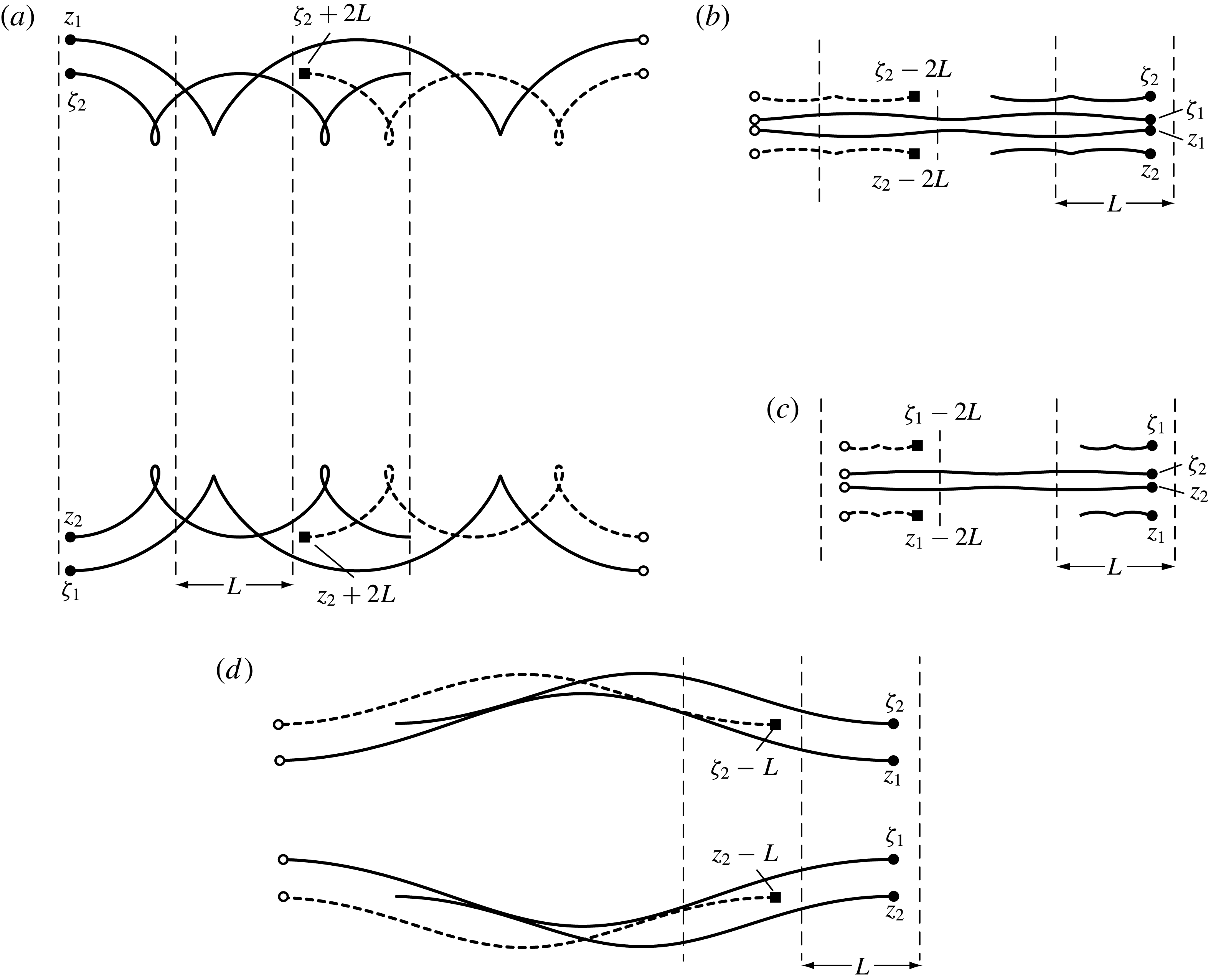
There are several regions in phase space for which, as the relative vortex motion progresses in time,
 $|X|$
increases without bound while
 $|Y|$
stays bounded, and the net motion of all vortices in physical space is in the same general direction along the
 $x$
axis. The vortices from initially close pairs travel at significantly different speeds in the
 $x$
direction, leading to the original vortex pairs ‘exchanging partners’ with neighbouring image pairs and the separation between vortices
 $z_{1}$
and
 $z_{2}$
growing without bound. The initial vortex arrangement is repeated periodically in time, but with an exchange of the vortices that constitute that arrangement. We thus refer to these regimes of motion as exchanging regimes and label them
 $E_{i}$
,
 $i=1,2,3,4$
, as illustrated in panels I and III in figure 2. Representative examples of physical space vortex motion from these regimes are shown in figure 6.
Representative examples of exchanging motion in the singly periodic
 $(x,y)$
-plane with period
 $L$
. Initial conditions belong to the regimes (a)
 $E_{1}$
, (b)
 $E_{2}$
and (c)
 $E_{3}$
in panel III of figure 2 with
 $(\unicode[STIX]{x1D6FE},{\mathcal{P}})=(3/7,-1)$
and (d)
 $E_{4}$
in panel I of figure 2 with
 $(\unicode[STIX]{x1D6FE},{\mathcal{P}})=(3/7,-3/2)$
. Solid circles mark initial locations of base vortices, labelled according to the vortex definitions in figure 1; solid lines trace out vortex pathlines. Solid squares mark the initial locations of image vortices, and heavy dashed lines trace out the pathlines of these image vortices. Open circles mark the reconstituted vortex configurations after two periods of relative motion for each of (a–c), and after one period for (d). The
 $x$
and
 $y$
axes are all shown to the same scale.

In regime
 $E_{1}$
, representative real space trajectories of which are shown in figure 6(a), the vortex separation
 $Z$
evolves from left to right, with
 $X$
increasing without bound over time and
 $Y$
remaining large and positive but bounded. The
 $E_{1}$
regime is one of the two exchanging regimes (along with
 $E_{4}$
, discussed later) that is not bounded in the
 $(X,Y)$
plane by the singularities that occur along the H
 $_{1}$
, H
 $_{2}$
lines. In physical space, the net motion of each vortex is to the right. Owing to the inequality of the vortex strengths and the separation of the pairs, the paired real space vortices attempt to move together on circular paths. As the corresponding phase space trajectory passes near the fixed point D (or one of its periodic images), the paired base vortices and their period images approach becoming co-linear in an arrangement that is close to the (unstable) relative equilibrium configuration in panel D of figure 3. How closely the vortex positions approach those in the equilibrium configuration depends, of course, on how closely the phase trajectory lies to the separatrix emanating from D. At this point the weaker vortices at
 $z_{1}$
and
 $\unicode[STIX]{x1D701}_{1}$
begin to interact with the strong image vortices at
 $\unicode[STIX]{x1D701}_{2}+L$
and
 $z_{2}+L$
, respectively, and pairs are exchanged.
In regime
 $E_{2}$
, representative trajectories of which are shown in figure 6(b), the net translation of each vortex is to the left. The two weak vortices at
 $z_{1}$
and
 $\unicode[STIX]{x1D701}_{1}$
are located quite close together near the wake centreline. This proximity, together with the influence of the strong (outer) vortices at
 $z_{2}$
and
 $\unicode[STIX]{x1D701}_{2}$
, push the vortices at
 $z_{1}$
and
 $\unicode[STIX]{x1D701}_{1}$
quickly to the left, leading to values of
 $X$
that decrease without bound. For the first reconstitution of the initial relative vortex arrangement, the faster vortices pair with slower vortices originating at a distance
 $L$
to the left.
In regime
 $E_{3}$
, the two strong (inner) vortices at
 $z_{2}$
and
 $\unicode[STIX]{x1D701}_{2}$
are very close to each other near the wake centreline, and they translate faster to the left than do the two (outer) weak vortices at
 $z_{1}$
and
 $\unicode[STIX]{x1D701}_{1}$
. Figure 6(c) shows representative trajectories of the vortices in physical space. This rapid motion of the strong vortices is a departure from the behaviour observed in the
 $E_{1}$
,
 $E_{2}$
and
 $E_{4}$
regimes, in which the weaker vortices propagate more quickly. The initial relative configuration first reconstitutes when the faster moving vortices pair with the slower vortices that were initially at a distance
 $L$
to the left.
In regime
 $E_{4}$
, representative physical trajectories of which are shown in figure 6(d), the two weaker (inner) vortices at
 $z_{1}$
and
 $\unicode[STIX]{x1D701}_{1}$
translate faster to the left than the stronger vortices, and
 $X$
decreases without bound. This regime is bounded by regimes
 $O_{1}$
and
 $O_{3}$
, and (like
 $E_{1}$
) is not constrained by an H
 $_{i}$
line of singularity.
2.4.3 Reverse exchanging motion
There also exist two regimes of motion for which, as in the exchanging regimes,
 $|X|$
increases without bound while
 $|Y|$
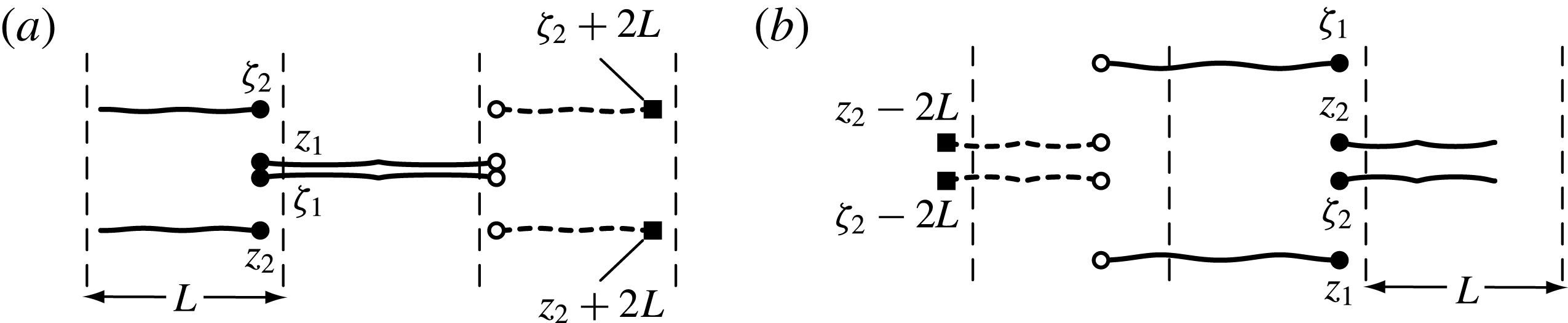
stays bounded. In contrast to the exchanging regimes, for these regimes the net motion of the vortices in physical space is not all in the same general direction. Representative examples of the physical space vortex motion from these regimes are shown in figure 7. Vortices from the initial configuration again travel at significantly different speeds in the
 $x$
direction, leading to exchanges of initial base vortex ‘pairs’ with neighbouring image ‘pairs’. However, the vortices further from the
 $x$
axis propagate in the opposite, or reverse, direction of the vortices closer to the
 $x$
axis. We thus refer to these regimes of motion as reverse exchanging regimes and label them
 $R_{1}$
and
 $R_{2}$
, as illustrated in panel III of figure 2. For
 $R_{1}$
,
 $X$
increases continually in time, and the weaker vortices
 $\{z_{1},\unicode[STIX]{x1D701}_{1}\}$
are closely spaced near the
 $x$
axis, as shown in figure 6(a). For
 $R_{2}$
,
 $X$
decreases with time, and the stronger vortices
 $\{z_{2},\unicode[STIX]{x1D701}_{2}\}$
are the ones near the
 $x$
axis, as shown in figure 6(b). In both regimes, the original vortex configuration is reformed for the first time by vortices that were initially separated in the
 $x$
direction by a distance
 $L$
. The regime
 $R_{1}$
(
 $R_{2}$
) is adjacent to the line of singularity at H
 $_{1}$
(H
 $_{2}$
) discussed in § 2.2, which is reached in the limit as
 $z_{1}\rightarrow \unicode[STIX]{x1D701}_{1}$
(
 $z_{2}\rightarrow \unicode[STIX]{x1D701}_{2}$
).
Representative examples of reverse exchanging motion for
 $(\unicode[STIX]{x1D6FE},{\mathcal{P}})=(3/7,-1)$
in the singly periodic
 $(x,y)$
-plane with period
 $L$
. Initial conditions belong to the regimes (a)
 $R_{1}$
and (b)
 $R_{2}$
, respectively, corresponding to the regimes labelled in panel III of figure 2. Solid circles mark initial vortex locations, labelled according to the vortex definitions in figure 1; solid lines trace out pathlines of these vortices. Solid squares mark the initial locations of image vortices, and short dashed lines trace out the pathlines of these image vortices. Hollow circles mark the reconstituted vortex configurations after two periods of relative motion. The
 $x$
and
 $y$
axes are all shown to the same scale.

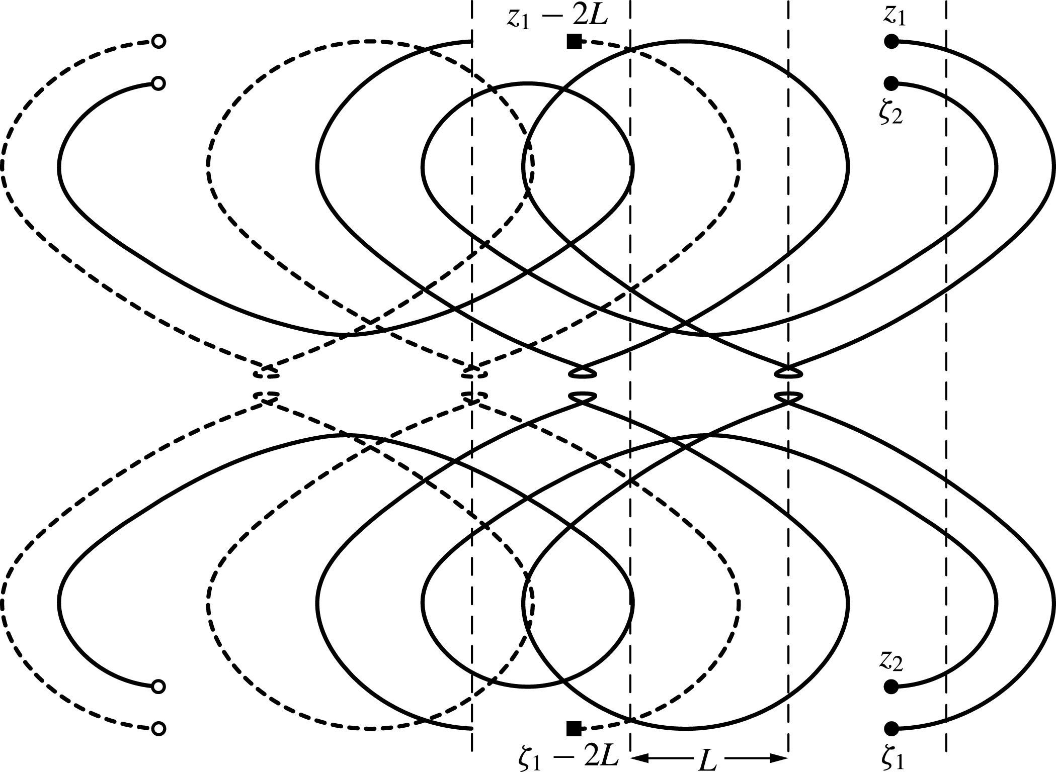
A representative example of mixed motion for
 $(\unicode[STIX]{x1D6FE},{\mathcal{P}})=(3/7,-1)$
in the singly periodic
 $(x,y)$
-plane with period
 $L$
. Initial conditions belong to the
 $M_{1}$
regime, as labelled in panel III of figure 2. Solid circles mark initial vortex locations, labelled according to the vortex definitions in figure 1; solid lines trace out pathlines of these vortices. Solid squares mark the initial locations of image vortices and short dashed lines trace out the pathlines of these image vortices. Hollow circles mark the reconstituted vortex configuration after two periods of relative motion. The
 $x$
and
 $y$
axes are shown to the same scale.

In the companion singly periodic system with four vortices having a glide-reflective symmetry (corresponding to
 $m=1$
), the vortices are always observed to translate in the same general direction and thus no reverse exchanging motion is found (Basu & Stremler Reference Basu and Stremler2015). However, similar reverse exchanging motion can be achieved in a singly periodic system of three point vortices, as can be seen by considering the regimes of motion labelled I and II in Aref & Stremler (Reference Aref and Stremler1996); in these cases, for which
 $|X|$
is relatively large, the net translation of one vortex is in the opposite direction of the other two.
2.4.4 Mixed motion
Finally, there is one regime in which the vortex motion exhibits properties akin to that in both orbiting and exchanging regimes. As in Basu & Stremler (Reference Basu and Stremler2015), we refer to this regime as a mixed motion regime; we label this regime
 $M_{1}$
, as illustrated in panel III of figure 2. Representative physical trajectories are shown in figure 8; the initial condition for this example is chosen to have the maximum
 $Y$
value along the corresponding
 $Z$
trajectory. Initially, the vortex pairs
 $\{z_{1},\unicode[STIX]{x1D701}_{2}\}$
and
 $\{z_{2},\unicode[STIX]{x1D701}_{1}\}$
appear to be orbiting one another as in regime
 $O_{1}$
. However, as the weaker vortices
 $\{z_{1},\unicode[STIX]{x1D701}_{1}\}$
approach the
 $x$
axis, they interact strongly and spend a brief period of time moving to the right while the stronger vortices
 $\{z_{2},\unicode[STIX]{x1D701}_{2}\}$
continue moving to the left. The stronger vortices then pair with the weaker vortices at
 $\{z_{1}-L,\unicode[STIX]{x1D701}_{1}-L\}$
, and these new pairs then orbit one another until again the weaker vortices interact, leading to another exchange, and so on.
3 The special cases
$\unicode[STIX]{x1D6FE}=0,1/2$

The representative example discussed in § 2 illustrates the general behaviour of this reflectively symmetric vortex system. This general description breaks down when we take
 $\unicode[STIX]{x1D6FE}=0$
or
 $\unicode[STIX]{x1D6FE}=1/2$
, corresponding to the special cases with
 $\unicode[STIX]{x1D6E4}_{1}=0$
or
 $\unicode[STIX]{x1D6E4}_{1}=\unicode[STIX]{x1D6E4}_{2}$
, respectively.
3.1 The special case
$\unicode[STIX]{x1D6FE}=0$

Choosing
 $\unicode[STIX]{x1D6FE}=0$
(equivalently,
 $\unicode[STIX]{x1D6E4}_{1}=0$
) leads us to the ‘restricted vortex problem’, in which the ‘vortices’ at
 $z_{1}$
and
 $\unicode[STIX]{x1D701}_{1}$
have zero circulation and thus are merely passive particles being advected by the two vortices (with non-zero strength) at
 $z_{2}$
and
 $\unicode[STIX]{x1D701}_{2}$
. The system therefore consists of just two rows of (finite strength) vortices with mirror symmetry about the centreline, horizontal (periodic) spacing
 $L$
between the like-signed vortices, and a vertical separation between the oppositely signed vortices of
 $2y_{2}={\mathcal{P}}L/\unicode[STIX]{x03C0}$
according to (1.10). As a result of this degeneracy, the Hamiltonian (1.3) is trivially a constant of the motion that gives no information regarding the relative vortex spacing
 $Z$
.
A Hamiltonian for this special case can be determined by considering that
 $z_{1}$
and
 $\unicode[STIX]{x1D701}_{1}$
represent the positions of passive particles that do not influence the behaviour of the point vortices at
 $z_{2}$
and
 $\unicode[STIX]{x1D701}_{2}$
. The vortices
 $\{z_{2},\unicode[STIX]{x1D701}_{2}\}$
move steadily in relative equilibrium with speed
 $$\begin{eqnarray}{\mathcal{U}}=\frac{1}{2L\text{i}}\unicode[STIX]{x1D6E4}_{2}\cot \left[\frac{\unicode[STIX]{x03C0}}{L}(\unicode[STIX]{x1D701}_{2}-z_{2})\right]=\frac{\unicode[STIX]{x1D6E4}_{2}}{2L}\coth ({\mathcal{P}})\end{eqnarray}$$
in the
 $x$
direction, as determined by (1.1). The variable
 $Z$
represents the dimensionless position of the passive particle at
 $z_{1}$
in a frame of reference that moves with the equilibrium vortex configuration. Thus, level curves for the relative ‘vortex’ motion in the
 $Z$
plane are equivalent (for
 $L=\unicode[STIX]{x03C0}$
) to streamlines of the flow generated by vortices
 $\{z_{2},\unicode[STIX]{x1D701}_{2}\}$
in a co-moving frame with background velocity
 $-{\mathcal{U}}$
(3.1). The streamfunction for the flow generated by vortices
 $\{z_{2},\unicode[STIX]{x1D701}_{2}\}$
in the co-moving frame is given by
 $$\begin{eqnarray}\unicode[STIX]{x1D713}(x,y)=\frac{-\unicode[STIX]{x1D6E4}_{2}}{2L}\ln \left|\frac{\sin [\unicode[STIX]{x03C0}(z-z_{2})/L]}{\sin [\unicode[STIX]{x03C0}(z-\unicode[STIX]{x1D701}_{2})/L]}\right|-{\mathcal{U}}y,\end{eqnarray}$$
where
 $z=x+\text{i}y$
gives the location of a passive particle advected by the vortices. The (dimensionless) Hamiltonian representing the special case
 $\unicode[STIX]{x1D6FE}=0$
can thus be written as
 $$\begin{eqnarray}\hat{{\mathcal{H}}}(Z;{\mathcal{P}})=-\frac{1}{2\unicode[STIX]{x03C0}}\left[\ln \left|\frac{\sin ^{2}X+\sinh ^{2}Y}{\sin ^{2}X+\sinh ^{2}[{\mathcal{P}}+Y]}\right|+2\coth ({\mathcal{P}})Y\right],\end{eqnarray}$$
where here
 $Z=\unicode[STIX]{x03C0}(z_{1}-z_{2})/L=\unicode[STIX]{x03C0}(z-z_{2})/L$
.
Representative level curves of
 $\hat{{\mathcal{H}}}$
on the
 $(X,Y)$
-plane (
 $W=\unicode[STIX]{x03C0}$
) and, equivalently, streamlines on the
 $(x,y)$
-plane (
 $W=L$
) for
 $\unicode[STIX]{x1D6FE}=0$
and various values of
 $|{\mathcal{P}}|$
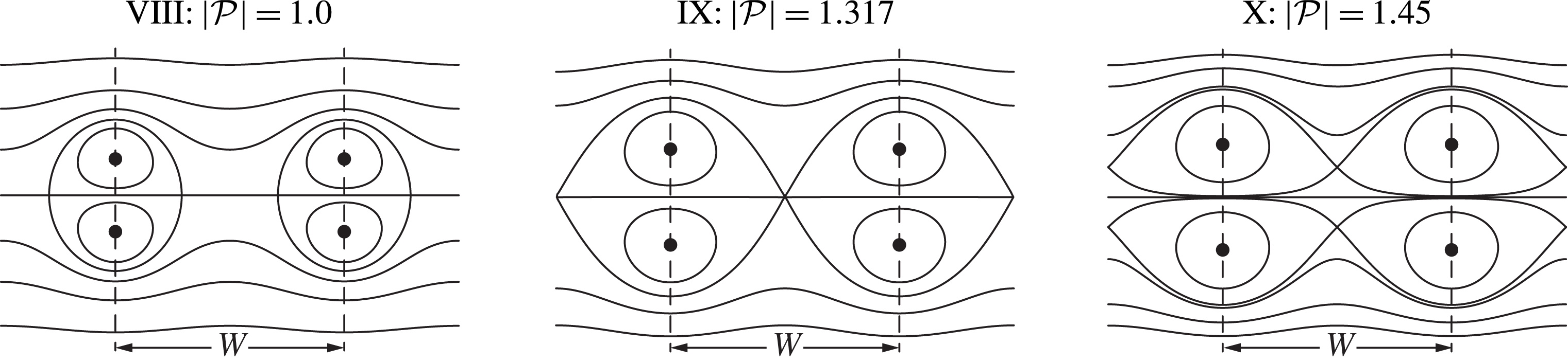
. Circles show fixed points and, equivalently, vortices; heavy lines show separatrices. Panels are labelled by Roman numerals VIII–X and the corresponding values of
 ${\mathcal{P}}$
. Each panel shows two periods for clarity. Horizontal and vertical axes are all shown to the same scale.

Representative level curves of the Hamiltonian in (3.3) and, equivalently, representative stream lines for the streamfunction in (3.2) are shown in figure 9. Three distinct types of level curve topology exist for
 $\unicode[STIX]{x1D6FE}=0$
. For
 $|{\mathcal{P}}|=|{\mathcal{P}}_{IX}|\approx 1.3168$
, there is one degenerate saddle fixed point (per period) at
 $(X,Y)=(\unicode[STIX]{x03C0}/2,-{\mathcal{P}}/2)$
. For
 $0<|{\mathcal{P}}|<|{\mathcal{P}}_{IX}|$
, there are two saddle fixed points (per period) along the line
 $Y=-{\mathcal{P}}/2$
, and the level curve topology is consistently as shown in example VIII. For
 $|{\mathcal{P}}|>|{\mathcal{P}}_{IX}|$
, the two saddle fixed points lie instead along the vertical line
 $X=\unicode[STIX]{x03C0}/2$
, and panel X of figure 9 shows the level curve topology for this range of
 ${\mathcal{P}}$
values. The case
 ${\mathcal{P}}=0$
is a degenerate case in which the vortices at
 $z_{2}$
and
 $\unicode[STIX]{x1D701}_{2}$
coincide and cancel each other out.
In the limit as
 $\unicode[STIX]{x1D6FE}\rightarrow 0$
, the line
 $\text{H}_{1}$
becomes the horizontal line at
 $Y={\mathcal{P}}/2$
. In contrast to all other cases, with
 $\unicode[STIX]{x1D6FE}=0$
there is no singularity when taking
 $z_{1}=\unicode[STIX]{x1D701}_{1}$
, so
 $\text{H}_{1}$
is merely a level curve in this case. The line
 $\text{H}_{2}$
still corresponds to the singularity that occurs with taking
 $z_{2}=\unicode[STIX]{x1D701}_{2}$
, but this line is now located at
 $Y\rightarrow (\text{sgn}\,{\mathcal{P}})\infty$
.
3.2 The special case
$\unicode[STIX]{x1D6FE}=1/2$

When all the vortex strengths are equal in magnitude, we have
 $\unicode[STIX]{x1D6FE}=1/2$
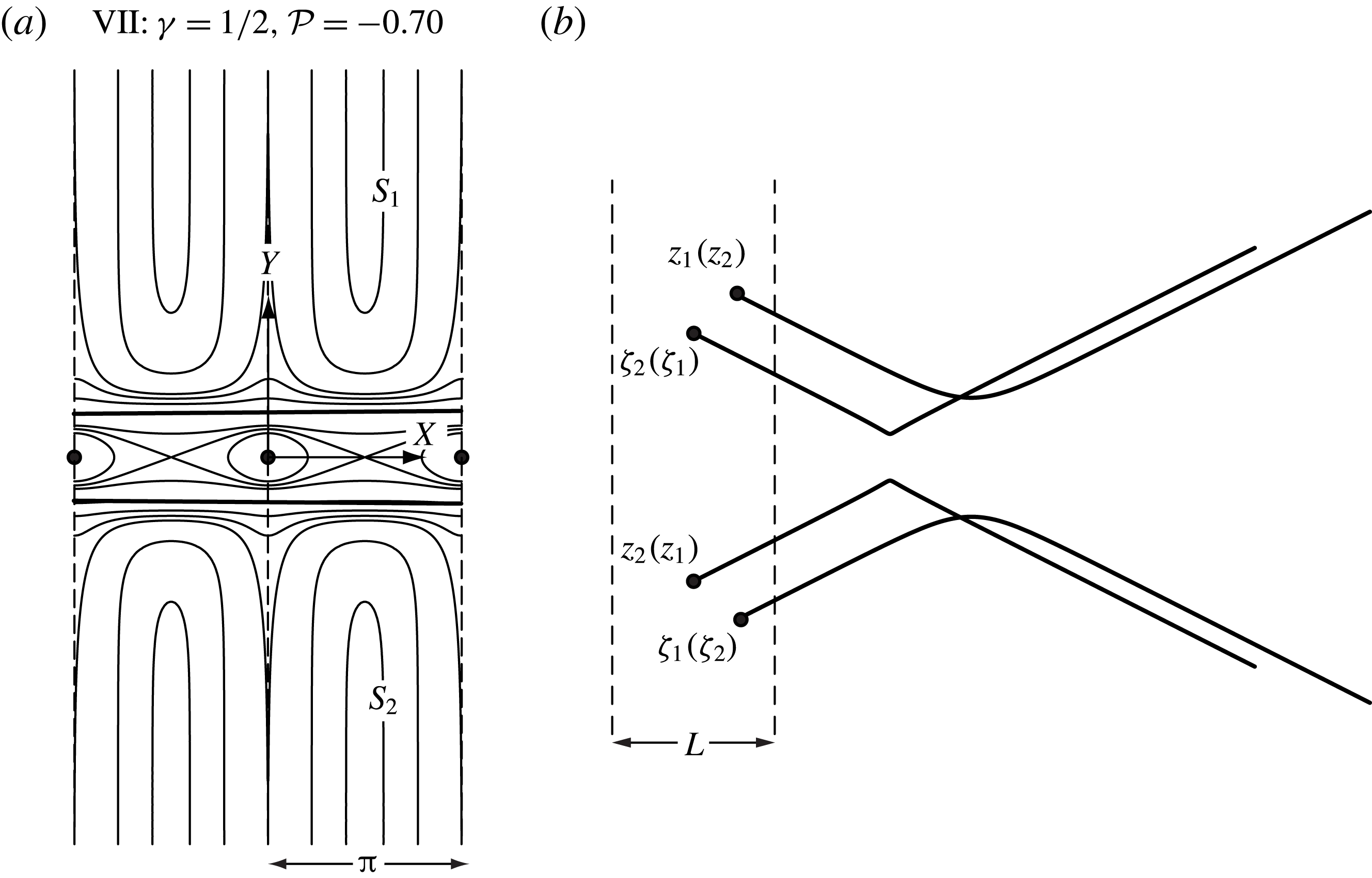
, and the phase space topology becomes that shown in figure 10(a). For this representative case, we have arbitrarily chosen
 $|{\mathcal{P}}|=0.70$
. Owing to the vortex strength equivalence, an inherent symmetry is observed in the phase domain on the
 $Z$
-plane. All fixed points but B and E move to
 $|Y|\rightarrow \infty$
in this case, giving new regimes of motion in which vortex configurations with initially finite values of
 $Y$
have unbounded separation. We refer to these regimes as the scattering modes
 $S_{1}$
and
 $S_{2}$
. In real space, vortex pairs consisting of oppositely signed vortices approach each other from opposite sides of the wake centreline before eventually diverging away with
 $Y\rightarrow \pm \infty$
. Figure 10(b) gives examples of the real space trajectories for the two scattering regimes. Similar scattering motion also occurs with staggered 2P arrangements (Stremler et al.
Reference Stremler, Salmanzadeh, Basu and Williamson2011; Basu & Stremler Reference Basu and Stremler2015).
(a) Selected level curves of
 ${\mathcal{H}}$
in the
 $(X,Y)$
phase space for
 $\unicode[STIX]{x1D6FE}=1/2$
and
 ${\mathcal{P}}=-0.70$
. The phase space is labelled VII according to the corresponding point in figure 11. The scattering mode regimes are labelled
 $S_{1}$
,
 $S_{2}$
. (b) Representative vortex trajectories corresponding to the
 $S_{1}$
(
 $S_{2}$
) regimes. Solid circles mark the initial locations of the vortices. The boundaries on the periodic strip are shown with dashed lines, and the solid lines represent the vortex trajectories. The absolute starting positions of the vortices in the
 $(x,y)$
-plane are chosen arbitrarily. The horizontal and vertical axes are shown to the same scale in (a) and (b), respectively.

4 Bifurcations in phase space topology
If we consider the phase space level curve topology for different values of
 ${\mathcal{P}}$
at a representative value of
 $\unicode[STIX]{x1D6FE}$
, as illustrated in figure 2 for
 $\unicode[STIX]{x1D6FE}=3/7$
, a sequence of distinct changes are observed. For large values of
 $|{\mathcal{P}}|$
, there is a large vertical separation between the neutrally stable fixed points A and C, and the saddle fixed points D and F are joined to their (respective) periodic images by separatrices; an example is shown in figure 2 for
 ${\mathcal{P}}=-1.5$
. As shown in panel II of figure 2, the saddle fixed points D and F themselves become connected by separatrices when
 $|{\mathcal{P}}|=|{\mathcal{P}}_{II}|\approx 1.167$
, a topology that we refer to as a saddle bifurcation. When the value of
 ${\mathcal{P}}$
is perturbed to be less than
 ${\mathcal{P}}_{II}$
, D and F each have a homoclinic orbit, with one of the separatrices from each point forming a closed loop. As
 ${\mathcal{P}}$
decreases, the saddle point at D and the elliptic point at C (along with their periodic images) gradually approach each other until they coincide, as shown in panel IV of figure 2 for
 ${\mathcal{P}}={\mathcal{P}}_{IV}\approx -0.495$
, producing a cusp in the corresponding phase trajectory. We refer to this level curve topology as a cusp bifurcation. For
 $|{\mathcal{P}}|<|{\mathcal{P}}_{IV}|$
, the fixed points C and D (and their periodic counterparts) do not appear in phase space, as illustrated in panel V of figure 2.
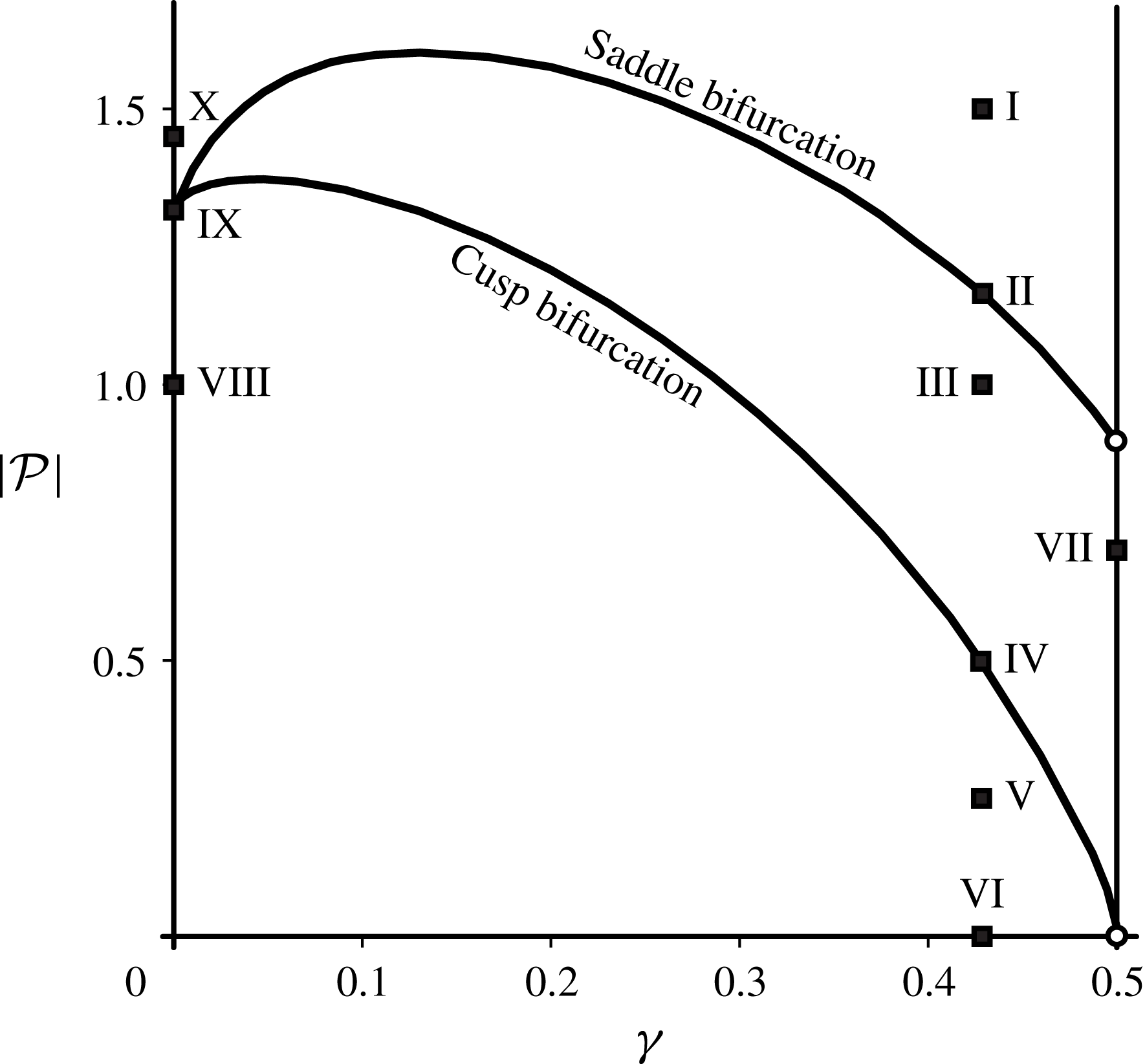
Bifurcation diagram for the phase space topology. Solid lines mark the
 $(\unicode[STIX]{x1D6FE},{\mathcal{P}})$
coordinates at which phase space fixed points D and F are connected by separatrices (saddle bifurcation) or where fixed points C and D coincide (cusp bifurcation). Square markers, labelled I–X, correspond to the phase space examples shown in figures 2, 9 and 10. Point IX marks the parameter values for which there exists a degenerate saddle point, as discussed in § 3.1. The hollow circles indicate that the saddle and cusp bifurcations do not occur for finite values of
 $Y$
when
 $\unicode[STIX]{x1D6FE}=1/2$
.

To extract the
 $(\unicode[STIX]{x1D6FE},{\mathcal{P}})$
values corresponding to phase space bifurcations, we varied
 $\unicode[STIX]{x1D6E4}_{1}$
over the range
 $[0,1]$
with an increment of 0.01 while keeping
 $\unicode[STIX]{x1D6E4}_{2}=1$
. For each resulting selection of
 $\unicode[STIX]{x1D6FE}\in [0,1/2]$
and for an initial trial value of
 ${\mathcal{P}}$
, we numerically solved
 $\unicode[STIX]{x2202}{\mathcal{H}}/\unicode[STIX]{x2202}X=\unicode[STIX]{x2202}{\mathcal{H}}/\unicode[STIX]{x2202}Y=0$
using Wolfram Mathematica™ to determine the positions of points C, D and F in the
 $(X,Y)$
plane. These positions were used in equation (1.12) to determine values
 ${\mathcal{H}}_{C}$
,
 ${\mathcal{H}}_{D}$
and
 ${\mathcal{H}}_{F}$
, respectively. The value of
 ${\mathcal{P}}$
was varied iteratively until either
 $\unicode[STIX]{x1D6E5}_{1}={\mathcal{H}}_{D}-{\mathcal{H}}_{F}\approx 0$
or
 $\unicode[STIX]{x1D6E5}_{2}={\mathcal{H}}_{D}-{\mathcal{H}}_{C}\approx 0$
, to an accuracy of at least three digits in
 ${\mathcal{P}}$
. Finding
 $\unicode[STIX]{x1D6E5}_{1}=0$
gives the saddle bifurcation and
 $\unicode[STIX]{x1D6E5}_{2}=0$
gives the cusp bifurcation.
Figure 11 shows all possible values of
 $(\unicode[STIX]{x1D6FE},{\mathcal{P}})$
for which bifurcations occur in the phase space level curve topology. When
 $0<\unicode[STIX]{x1D6FE}<1/2$
, the possible phase space topologies are fully represented by the examples shown in figure 2. For
 $\unicode[STIX]{x1D6FE}=0$
, the bifurcation curves intersect at point IX, with
 ${\mathcal{P}}_{IX}\approx 1.3168$
, giving the level curve topology shown in panel IX of figure 9; all possible phase space topologies for
 $\unicode[STIX]{x1D6FE}=0$
are shown in figure 9. When
 $\unicode[STIX]{x1D6FE}=1/2$
, the fixed points involved in these bifurcations all lie at
 $Y\rightarrow \pm \infty$
. Thus there are no bifurcations in the phase space topology for
 $\unicode[STIX]{x1D6FE}=1/2$
, and this choice of
 $\unicode[STIX]{x1D6FE}$
is fully represented by the example in figure 10. In comparison with the bifurcation diagram for the staggered 2P system (Basu & Stremler Reference Basu and Stremler2015), the presence of the horizontal lines H
 $_{1}$
and H
 $_{2}$
limits the number of bifurcations that can occur.
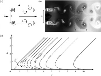
(a) An illustration of symmetric vortex wake formation behind two circular cylinders with transverse separation
 $h$
in a uniform background flow with speed
 $U$
. (b) An example of a symmetric 2P wake from Fayed et al. (Reference Fayed, Portaro, Gunter, Abderrahmane and Ng2011). The estimated spatial period is marked with dashed lines; cylinder locations and estimated vortex core locations are marked with large and small open circles, respectively. The measured cylinder and vortex separations are
 $h\approx 2.96L/\unicode[STIX]{x03C0}$
and
 $b\approx 0.92L/\unicode[STIX]{x03C0}$
. (c) Contour plots of the non-dimensional transverse separations between the paired vortices,
 $B$
, as a function of the transverse separation between the wake shedding cylinders,
 $Y$
, for different values of
 $\unicode[STIX]{x1D6FE}$
as noted on each curve. The starting point of each contour is marked by a solid circle; arrows indicate that the curves extend monotonically to infinity. The hollow square corresponds to the experiment in (b), and the dashed curve is the
 $\unicode[STIX]{x1D6FE}$
contour passing through that point.

5 Comparison with experiments
The point-vortex model presented here allows for comparisons with experimental results under certain conditions. The more straightforward comparison is with wakes assumed to have vortices arranged close to a relative equilibrium configuration. We consider one such comparison in § 5.1. Comparisons with wakes in which the vortices exhibit noticeable relative motion are also possible, but a transformation must be made between the spatially periodic point-vortex motions in the model and the physical wakes. An example comparison with vortex motion is discussed in § 5.2.
5.1 Neutrally stable relative equilibria shed from two bluff bodies
As pointed out in § 2.1, point C in the phase plane corresponds to a relative equilibrium configuration in which the symmetric array of four vortices (per spatial period) moves without any change in relative position. The apparent stability of this configuration, discussed in § 2.3, suggests that such a vortex arrangement should be observable in experiments. As illustrated in figure 12, the vortex pattern in this equilibrium configuration is indeed similar to that observed in adjacent von Kármán wakes of two closely spaced bluff bodies. If we assume this cylinder arrangement produces a wake that is at (or close to) an equilibrium state, the point-vortex model can relate the cylinder spacing and vortex positions to the vortex circulation ratio.
Following the standard notation for a von Kármán street, let
 $b$
be the spanwise separation between the vortices in each pair, giving
 $$\begin{eqnarray}b=\text{Im}(\unicode[STIX]{x1D701}_{2}-z_{1})=\text{Im}(\unicode[STIX]{x1D701}_{1}-z_{2})=-(y_{1}+y_{2}).\end{eqnarray}$$
Using (1.10), this transverse separation can be non-dimensionalized as
 $$\begin{eqnarray}B=\frac{\unicode[STIX]{x03C0}b}{L}=-[{\mathcal{P}}+(1-2\unicode[STIX]{x1D6FE})Y].\end{eqnarray}$$
We assume that the cylinders lie medially spanwise between the vortices in each pair. Thus, the inter-cylinder transverse spacing is
 $$\begin{eqnarray}h=2y_{1}+b=\frac{LY}{\unicode[STIX]{x03C0}},\end{eqnarray}$$
where we have made use of equations (1.10) and (5.1). Applying this perspective to the experiment by Fayed et al. (Reference Fayed, Portaro, Gunter, Abderrahmane and Ng2011), as shown in figure 12(b), yields
 $(Y,B)\equiv (2.96,0.92)$
.
As discussed in § 2.1, point C is a neutrally stable fixed point with
 $X_{C}=(2n+1)\unicode[STIX]{x03C0}/2$
. For given values of
 $(\unicode[STIX]{x1D6FE},{\mathcal{P}})$
, the correspondence of point C with a relative equilibrium configuration allows for determination of
 $Y_{C}$
by numerical solution of
 $$\begin{eqnarray}\left.\frac{\unicode[STIX]{x2202}{\mathcal{H}}}{\unicode[STIX]{x2202}Y}\right|_{X=X_{C},Y=Y_{C}}=\left.\frac{\unicode[STIX]{x2202}{\mathcal{H}}}{\unicode[STIX]{x2202}X}\right|_{X=X_{C},Y=Y_{C}}=0,\end{eqnarray}$$
subject to the following constraints: (i) the neutral stability of C requires that the Hessian of
 ${\mathcal{H}}$
maintain
 $$\begin{eqnarray}\left.\left(\frac{\unicode[STIX]{x2202}^{2}{\mathcal{H}}}{\unicode[STIX]{x2202}X^{2}}\right)\left(\frac{\unicode[STIX]{x2202}^{2}{\mathcal{H}}}{\unicode[STIX]{x2202}Y^{2}}\right)-\left(\frac{\unicode[STIX]{x2202}^{2}{\mathcal{H}}}{\unicode[STIX]{x2202}X\unicode[STIX]{x2202}Y}\right)\left(\frac{\unicode[STIX]{x2202}^{2}{\mathcal{H}}}{\unicode[STIX]{x2202}Y\unicode[STIX]{x2202}X}\right)\right|_{X=X_{C},Y=Y_{C}}>0,\end{eqnarray}$$
and (ii)
 $|{\mathcal{P}}|$
must be greater than the value at which the cusp bifurcation occurs for the corresponding value of
 $\unicode[STIX]{x1D6FE}$
.
Solving for
 $Y=Y_{C}$
using (5.3) with given values of
 $(\unicode[STIX]{x1D6FE},{\mathcal{P}})$
determines
 $b$
(5.1) and
 $h$
(5.2). However, as we have already seen,
 $b$
and
 $h$
are the parameters most easily observed in a wake experiment. It is thus the inverse problem that is the more interesting: given values of
 $h$
and
 $b$
, and therefore fixing
 $Y$
, what value of
 $\unicode[STIX]{x1D6FE}$
satisfies (5.3)? By (1.12) and (5.3), determining
 $\unicode[STIX]{x1D6FE}$
for a given value of
 $Y$
also determines
 ${\mathcal{P}}$
. For the experiment in figure 12(b) with
 $(Y,B)\equiv (2.96,0.92)$
, or more precisely
 $(2.9569,0.9202)$
, the solution of this inverse problem gives
 $\unicode[STIX]{x1D6FE}=0.4845$
, thereby suggesting a circulation ratio of
 $\unicode[STIX]{x1D6E4}_{1}/\unicode[STIX]{x1D6E4}_{2}\approx 0.94$
for the wake vortices. In figure 12(c) we present level curves in the
 $(Y,B)$
plane along which equation (5.3a
) and the associated constraints are satisfied for constant values of
 $\unicode[STIX]{x1D6FE}$
. The lower bound on each curve is determined by occurrence of the cusp bifurcation. As
 $\unicode[STIX]{x1D6FE}\rightarrow 0$
, the contours tend to coalesce together; as
 $\unicode[STIX]{x1D6FE}\rightarrow 1/2$
, C moves to
 $Y\rightarrow \infty$
, causing the contours to become more and more separated. This diagram promises to be a convenient tool to gauge the relative strengths of the wake vortices in the case of similar stable co-existence of two neighbouring von Kármán streets shed by two closely separated bluff bodies.
5.2 On the connection between the model trajectories and an experimental wake
The rich variety of motions displayed by this point-vortex model provides motivation for determining the extent to which this behaviour can be observed in an experimental wake. We explore the connection between our model and real wakes by focusing on the experimental wake shown in figure 1(b). This wake is generated by two counter-rotating cylinders with equal diameter
 $d=0.635~\text{cm}$
in a water tunnel at a Reynolds number
 $Re=U_{e}d/\unicode[STIX]{x1D708}=200$
, corresponding to a mean flow speed
 $U_{e}\approx 3.15~\text{cm}~\text{s}^{-1}$
.
The point-vortex model is not a direct representation of an experimental wake with finite length. For mathematical tractability, the modelled motion of the
 $N=4$
base vortices is tied to interaction with their spatially periodic images, and each successive set of four vortices simultaneously depicts the same dynamics. This infinite collection of point vortices moves about in an inviscid fluid that is otherwise at rest. In a real wake, in contrast, successive clusters of four vortices are shed from the bluff bodies at regular intervals, and these vortices exhibit both spatial and temporal evolution as they are swept downstream by a flow moving with speed
 $U_{\infty }$
. Vorticity is concentrated in distinct structures, but the distribution of vorticity is continuous, not singular. Viscosity leads both to vortex formation and to dissipation of vorticity with increasing time.
A number of assumptions must be made in order to compare the dynamics in these two systems. First, we represent the locations of each experimental vortex as a point at the estimated centre of the vortex core, as illustrated in figure 1(b). The successive sets of four vortices we refer to as cluster
 $k=1,2,\ldots ,K$
, with
 $k=1$
representing the first distinct cluster adjacent to the bluff bodies and with
 $K=4$
clusters in this system. The position of each experimental vortex in the laboratory frame we label
 $\hat{z}_{\unicode[STIX]{x1D6FC},k}=\hat{x}_{\unicode[STIX]{x1D6FC},k}+\text{i}{\hat{y}}_{\unicode[STIX]{x1D6FC},k}$
(
 $\unicode[STIX]{x1D6FC}=1,\ldots ,4;k=1,\ldots ,K$
) according to the assumed sign and relative magnitude of the vortex circulation, with
 $$\begin{eqnarray}\left.\begin{array}{@{}c@{}}\displaystyle \unicode[STIX]{x1D6E4}_{3}=-\unicode[STIX]{x1D6E4}_{1},\quad \hat{z}_{3,k}\approx \hat{z}_{1,k}^{\ast },\\ \displaystyle \unicode[STIX]{x1D6E4}_{4}=-\unicode[STIX]{x1D6E4}_{2},\quad \hat{z}_{4,k}\approx \hat{z}_{2,k}^{\ast },\end{array}\right\}\end{eqnarray}$$
following (1.6). While the directions of the circulations are clear from the experimental image, the relative circulation magnitudes are less certain, so the fitting procedure is performed for both possible choices of
 $\hat{z}_{1,k}$
and
 $\hat{z}_{2,k}$
. The average spacing of the vortices is used to determine the effective spatial period of the experimental system,
 $$\begin{eqnarray}L_{e}=\frac{1}{4(K-1)}\mathop{\sum }_{\unicode[STIX]{x1D6FC}=1}^{4}\mathop{\sum }_{k=1}^{K-1}|\hat{x}_{\unicode[STIX]{x1D6FC},k+1}-\hat{x}_{\unicode[STIX]{x1D6FC},k}|,\end{eqnarray}$$
which we calculate to be
 $L_{e}=2.82~\text{cm}$
.
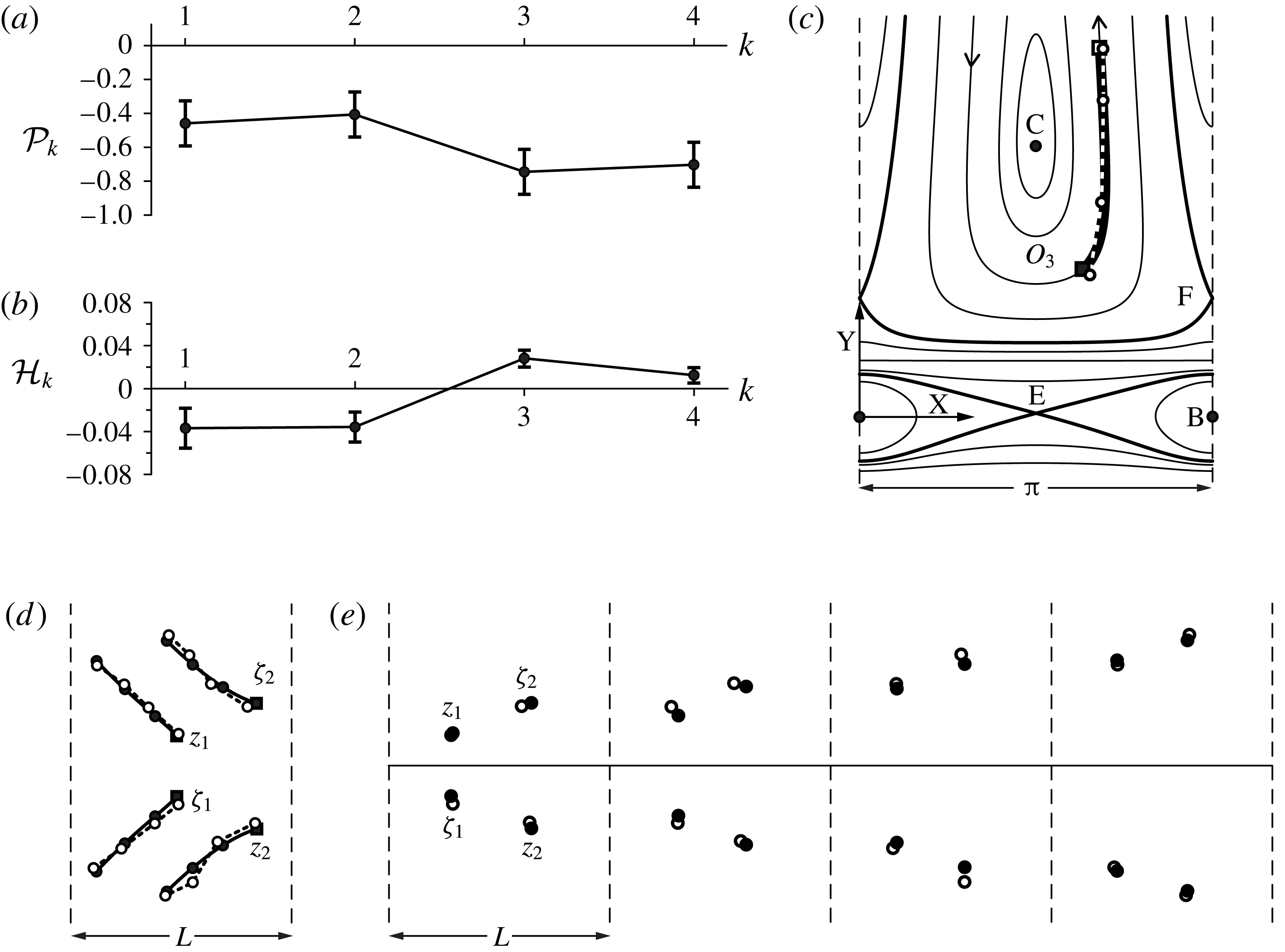
Values of the model constants (a)
 ${\mathcal{P}}_{k}$
and (b)
 ${\mathcal{H}}_{k}$
based on the locations of the experimental vortices in figure 1(b) for the circulation ratio
 $\unicode[STIX]{x1D6FE}=0.455$
. Values on the
 $x$
axis indicate cluster number. Error bars are determined by considering maximum fluctuations of
 $d/4$
from the assumed point-vortex locations. (c) Model phase space representation for
 $\unicode[STIX]{x1D6FE}=0.455$
and
 ${\mathcal{P}}=\bar{{\mathcal{P}}}_{\unicode[STIX]{x1D6FE}=0.455}=-0.578$
. Experimental data points
 $Z_{i}$
are shown with hollow circles and a dashed line; the thick solid line marks the best-fit model trajectory along
 ${\mathcal{H}}(Z;\unicode[STIX]{x1D6FE},\bar{{\mathcal{P}}}_{\unicode[STIX]{x1D6FE}})=\bar{{\mathcal{H}}}_{\unicode[STIX]{x1D6FE}}=-7.99\times 10^{-3}$
. The beginning and end of the model trajectory, corresponding to projections of
 $Z_{1}$
and
 $Z_{4}$
onto the model curve, are shown with a solid and hollow square, respectively. Arrows indicate direction of the phase space evolution. (d) Model vortex trajectories (solid lines) and experimental vortex positions at
 $z_{\unicode[STIX]{x1D6FC},k}$
(hollow circles connected by dashed lines) in a co-moving frame of reference with zero background velocity for
 $\unicode[STIX]{x1D6E4}_{1}\approx 2.81~\text{cm}^{2}~\text{s}^{-1}$
and
 $\unicode[STIX]{x1D6E4}_{2}\approx 3.36~\text{cm}^{2}~\text{s}^{-1}$
. Solid squares mark the initial locations of the model vortices, and solid circles mark the model vortex locations at times corresponding to the experimental shedding period. (e) Model predictions of the vortex locations (solid circles), with the added displacement provided by the free stream, superimposed on the estimated vortex locations from figure 1(b) (hollow circles). The horizontal and vertical axes in (d–e) are shown to the same scale.

Next we assume a value for
 $\unicode[STIX]{x1D6FE}$
and use the experimental vortex locations to determine corresponding values for the constants of motion needed in the model. For each cluster
 $k$
, the positions of vortices
 $\hat{z}_{1,k}$
and
 $\hat{z}_{2,k}$
in the co-moving frame are used in (1.9c,d
) with
 $L=L_{e}$
to determine corresponding values
 $$\begin{eqnarray}{\mathcal{P}}_{k}(\unicode[STIX]{x1D6FE})={\mathcal{P}}({\hat{y}}_{1,k},{\hat{y}}_{2,k};\unicode[STIX]{x1D6FE}),\end{eqnarray}$$
as shown in figure 13(a). The average value,
 $$\begin{eqnarray}\bar{{\mathcal{P}}}_{\unicode[STIX]{x1D6FE}}=\frac{1}{K}\mathop{\sum }_{k=1}^{K}{\mathcal{P}}_{k}(\unicode[STIX]{x1D6FE}),\end{eqnarray}$$
is taken as the representative experimental value for
 ${\mathcal{P}}$
, which specifies the phase plane topology in the corresponding model system for the selected value of
 $\unicode[STIX]{x1D6FE}$
. Error bounds on the
 ${\mathcal{P}}_{k}(\unicode[STIX]{x1D6FE})$
are determined by considering the error associated with defining the locations of the experimental vortices. For the errors shown in figure 13(a), the vortex locations were varied over the circles shown in figure 1(b), each with diameter
 $d/2$
. A similar procedure is used with equation (1.12) to determine
 $$\begin{eqnarray}{\mathcal{H}}_{k}(\unicode[STIX]{x1D6FE})={\mathcal{H}}(Z_{k};\unicode[STIX]{x1D6FE},\bar{{\mathcal{P}}}_{\unicode[STIX]{x1D6FE}}),\end{eqnarray}$$
such as illustrated in figure 13(b), where we have
 $$\begin{eqnarray}Z_{k}=\unicode[STIX]{x03C0}(\hat{z}_{1,k}-\hat{z}_{2,k})/L\end{eqnarray}$$
from applying (1.7). The average of the
 ${\mathcal{H}}_{k}(\unicode[STIX]{x1D6FE})$
,
 $$\begin{eqnarray}\bar{{\mathcal{H}}}_{\unicode[STIX]{x1D6FE}}=\frac{1}{K}\mathop{\sum }_{i=1}^{K}{\mathcal{H}}_{k}(\unicode[STIX]{x1D6FE}),\end{eqnarray}$$
gives the representative experimental value for
 ${\mathcal{H}}$
, which determines the relevant level curve in phase space from the model, as determined by
 ${\mathcal{H}}(Z;\unicode[STIX]{x1D6FE},\bar{{\mathcal{P}}}_{\unicode[STIX]{x1D6FE}})=\bar{{\mathcal{H}}}_{\unicode[STIX]{x1D6FE}}$
. The experimental phase space data and example model phase space curves are shown in figure 13(c).
The optimal value of
 $\unicode[STIX]{x1D6FE}$
is obtained by minimizing the differences between the experimental and model positions in phase space. Initial and final model positions are first determined by projecting
 $Z_{1}$
and
 $Z_{4}$
, respectively, onto the
 ${\mathcal{H}}(Z;\unicode[STIX]{x1D6FE},\bar{{\mathcal{P}}}_{\unicode[STIX]{x1D6FE}})=\bar{{\mathcal{H}}}_{\unicode[STIX]{x1D6FE}}$
curve, as illustrated in figure 13(c) by the square symbols. The system of equations (1.15) is then integrated between these two positions from
 $\unicode[STIX]{x1D70F}=0$
to
 $\unicode[STIX]{x1D70F}={\mathcal{T}}$
to determine the model integration time
 ${\mathcal{T}}$
and model positions
 $Z(\unicode[STIX]{x1D70F};\unicode[STIX]{x1D6FE})$
at times
 $\unicode[STIX]{x1D70F}=(k-1)\unicode[STIX]{x0394}\unicode[STIX]{x1D70F}$
,
 $k=1,\ldots ,K$
, with
 $\unicode[STIX]{x0394}\unicode[STIX]{x1D70F}={\mathcal{T}}/(K-1)$
. We use the notation
 $Z(\unicode[STIX]{x1D70F};\unicode[STIX]{x1D6FE})$
to emphasize that these model positions in phase space are dependent on the choice of
 $\unicode[STIX]{x1D6FE}$
. The error in the phase space fit between model and experiment is quantified by
 $$\begin{eqnarray}\mathbb{E}_{p}(\unicode[STIX]{x1D6FE})=\frac{1}{\unicode[STIX]{x03C0}}\left[\frac{1}{K}\mathop{\sum }_{k=1}^{K}|Z((k-1)\unicode[STIX]{x0394}\unicode[STIX]{x1D70F};\unicode[STIX]{x1D6FE})-Z_{k}|^{2}\right]^{1/2},\end{eqnarray}$$
where we have chosen to normalize by the phase space period,
 $\unicode[STIX]{x03C0}$
. We have determined that for this example
 $\mathbb{E}_{p}(\unicode[STIX]{x1D6FE})$
is minimized by taking
 $\unicode[STIX]{x1D6FE}=0.455$
with the vortex assignments shown in figure 1(c) (see also figure 13
d); this choice gives
 ${\mathcal{T}}=12.1$
,
 $\bar{{\mathcal{P}}}_{\unicode[STIX]{x1D6FE}}=-0.578$
,
 $\bar{{\mathcal{H}}}_{\unicode[STIX]{x1D6FE}}=-7.99\times 10^{-3}$
and
 $\mathbb{E}_{p}=0.0474$
. As shown in figure 13(c), the model-predicted vortex dynamics belongs to the
 $O_{3}$
regime (cf. § 2.4.1). Note that this phase space comparison assumes spatial symmetry in the experiment, so that only the positions of the vortices with positively signed circulation are used in the analysis.
The real space model vortex trajectories are then fitted to the experimental vortex locations in the co-moving frame, which includes determining the value of
 $\mathbb{S}$
and the optimal background flow speed,
 $U_{\infty }$
. We assume
 $U_{\infty }\approx U_{e}$
but consider uncertainty in the experimental background velocity as a free parameter by taking
 $$\begin{eqnarray}U_{\infty }=cU_{e}.\end{eqnarray}$$
For the example discussed here we explored
 $0.6\leqslant c\leqslant 1.5$
with a resolution of
 $\unicode[STIX]{x0394}c=10^{-4}$
.
A key step in the real-space fitting process involves transforming the spatially developing wake data into the temporal motion of four vortices. We assume that the experimental vortex shedding is exactly periodic in time, with a shedding frequency of
 $f_{e}$
. We assume a Strouhal number
 $$\begin{eqnarray}St=f_{e}d/U_{\infty }=0.2\end{eqnarray}$$
for this experimental system (Kumar, Cantu & Gonzalez Reference Kumar, Cantu and Gonzalez2011a
). The cluster
 $k$
will have moved to the position of cluster
 $k+1$
after an elapsed time
 $\unicode[STIX]{x0394}t=1/f_{e}$
owing to vortex interactions and a displacement of
 $U_{\infty }\unicode[STIX]{x0394}t$
caused by the background flow. The experimental vortex positions in a frame moving with the background flow are given by
 $$\begin{eqnarray}z_{\unicode[STIX]{x1D6FC},k}=\hat{z}_{\unicode[STIX]{x1D6FC},k}-kU_{\infty }\unicode[STIX]{x0394}t.\end{eqnarray}$$
These co-moving vortices can be viewed as showing temporal evolution of the four vortices initially from cluster
 $k=1$
. The motion of vortices from cluster 1 to cluster 4 is estimated to require an elapsed time of
 $T=(K-1)\unicode[STIX]{x0394}t$
. Comparing the model integration time
 ${\mathcal{T}}$
and the experimental elapsed time
 $T$
using equation (1.14) gives a scaled value for
 $\mathbb{S}$
in the experiment; together with the selected
 $\unicode[STIX]{x1D6FE}$
value, this
 $\mathbb{S}$
value gives an estimate for the experimental values of the vortex strengths.
Changing the assumed value of
 $U_{\infty }(c)$
by varying
 $c$
changes the experimental vortex positions in the co-moving frame,
 $z_{\unicode[STIX]{x1D6FC},k}$
; the experimental integration time,
 $T$
; and the dimensional value of
 $\mathbb{S}$
. For each value of
 $U_{\infty }(c)$
considered in our analysis, we quantify the difference between the experimental positions
 $z_{\unicode[STIX]{x1D6FC},k}$
, which depend on
 $c$
, and the corresponding model positions
 $z_{\unicode[STIX]{x1D6FC}}(t)=z_{\unicode[STIX]{x1D6FC}}((k-1)\unicode[STIX]{x0394}\unicode[STIX]{x1D70F})$
by computing
 $$\begin{eqnarray}\mathbb{E}_{r}(c)=\frac{1}{L_{e}}\left[\frac{1}{4K}\mathop{\sum }_{\unicode[STIX]{x1D6FC}=1}^{4}\mathop{\sum }_{k=1}^{K}|z_{\unicode[STIX]{x1D6FC}}((k-1)\unicode[STIX]{x0394}\unicode[STIX]{x1D70F})-z_{\unicode[STIX]{x1D6FC},k}(c)|^{2}\right]^{1/2},\end{eqnarray}$$
in which we have used the notation
 $z_{3}(t)=\unicode[STIX]{x1D701}_{1}(t)$
,
 $z_{4}(t)=\unicode[STIX]{x1D701}_{2}(t)$
. We determine the optimal value of
 $c$
by minimizing the error
 $\mathbb{E}_{r}(c)$
.
Figure 13(d) shows the resulting best-fit vortex trajectory comparison between the model predictions and the experiment from figure 1(b) in a co-moving frame of reference. As determined by our fitting procedure, in this comparison we have used a background flow speed
 $U_{\infty }=3.00~\text{cm}~\text{s}^{-1}$
(corresponding to
 $c=0.9537$
, or
 ${\sim}5\,\%$
difference from the initial
 $U_{e}$
value), giving an experimental elapsed time
 $T=3.17~\text{s}$
. By (1.14), we thus have
 $\mathbb{S}=6.17~\text{cm}^{2}~\text{s}^{-1}$
for the experiment; together with
 $\unicode[STIX]{x1D6FE}=0.455$
, this gives experimental values
 $\unicode[STIX]{x1D6E4}_{1}\approx 2.81~\text{cm}^{2}~\text{s}^{-1}$
and
 $\unicode[STIX]{x1D6E4}_{2}\approx 3.36~\text{cm}^{2}~\text{s}^{-1}$
. For this comparison,
 $\mathbb{E}_{r}=0.0747$
. Note that the comparison in real space does not assume spatial symmetry in the experiment, and the error
 $\mathbb{E}_{r}$
accounts for all of the experimental vortex positions. The translatory displacement owing to the background flow can also be superimposed on the model vortex evolutions, thereby enabling a comparison with the experiment in the laboratory frame of reference, as depicted in figure 13(e). Comparisons in both reference frames show a strong correspondence between the modelled vortex dynamics and the experimental data.
6 Conclusions
Here we have considered one of the few, and perhaps the last, remaining unsolved integrable problems in planar point-vortex dynamics. A singly periodic array of four point vortices with zero net strength are constrained by a reflective symmetry (1.6) and allowed to move under their mutual interactions in an inviscid, two-dimensional fluid that is otherwise at rest. The discrete symmetry constraint, which is preserved by the dynamics, enables the relative vortex motion to be represented as a Hamiltonian dynamical system (1.12) that depends on the relative vortex separation
 $Z$
(1.7); the relative vortex strengths, as represented by
 $\unicode[STIX]{x1D6FE}$
(1.8); and
 ${\mathcal{P}}$
(1.9), the (non-dimensional) transverse component of the linear impulse.
The Hamiltonian formulation allows the relative vortex motion to be given by level curves in the
 $(X,Y)$
phase space. Separatrices joining the saddle fixed points, together with the horizontal lines of singularity H
 $_{i}$
, separate the phase space into multiple regimes of motion. Within each regime the corresponding vortex motion is qualitatively similar, and the motions from different regimes can share similar characteristics. We have identified five general categories of relative vortex motion for this constrained system: orbiting motion (regimes
 $O_{1}$
,
 $O_{2}$
,
 $O_{3}$
), exchanging motion (regimes
 $E_{1}$
,
 $E_{2}$
,
 $E_{3}$
,
 $E_{4}$
), reverse exchanging motion (regimes
 $R_{1}$
,
 $R_{2}$
), mixed motion (regime
 $M_{1}$
) and scattering motion (regimes
 $S_{1}$
,
 $S_{2}$
).
Section 5.2 compares our model to a wake generated in a water tunnel. The similarity between the model trajectories and the experimental vortex evolution demonstrates that the vortex dynamics observed in our mathematical model does indeed appear to exist in a laboratory setting, at least for finite time. The richness of the model dynamics suggests that a mere statement on the number of vortices shed in each cycle, such as the classic classification by Williamson & Roshko (Reference Williamson and Roshko1988), is not sufficient for a comprehensive characterization of such complex (and beautiful) wake dynamics.
This vortex system is closely related to that considered by Stremler et al. (Reference Stremler, Salmanzadeh, Basu and Williamson2011), Stremler & Basu (Reference Stremler and Basu2014) and Basu & Stremler (Reference Basu and Stremler2015), in which a singly periodic array of four point vortices with zero net strength are constrained by a glide-reflective symmetry. Both systems contain instances of orbiting motion, exchanging motion, mixed motion and scattering motion. The passing motion observed in the glide-reflective system (Basu & Stremler Reference Basu and Stremler2015) is not allowed in the present system; reverse exchanging motion is found in the present system but not in the glide-reflective system. The presence of the singularities represented by the H
 $_{i}$
lines in the present system restricts the number of bifurcations that occur in the phase space topology, so that the glide-reflective system exhibits greater variation in behaviour with changes in the values of
 $(\unicode[STIX]{x1D6FE},{\mathcal{P}})$
.
The reflective system considered here also includes six different relative equilibrium configurations in which the vortices propagate in the
 $\pm x$
direction without any relative motion. One of these configurations, case C, is a neutrally stable arrangement of four vortices resembling the pattern that can be generated by two adjacent von Kármán (i.e. 2S) wakes. Neutral stability is proven here for perturbations that preserve the imposed spatial symmetry, and numerical experiments indicate that these configurations remain neutrally stable under symmetry breaking perturbations. With the geometry of the experimental wake pattern as input, our model predicts the ratios of the vortex strengths under the assumption that the system is at (or near) an equilibrium state. The glide-reflective system also has one neutrally stable equilibrium configuration of four vortices (Basu & Stremler Reference Basu and Stremler2015), for perturbations that are symmetry-preserving. The analysis approach used in § 5.1 for small
 $L$
-periodic symmetry-breaking perturbations has not yet been applied to that system. However, we note that the physical correspondence in the glide-reflective case is with two adjacent symmetric two-vortex wakes (Basu & Stremler Reference Basu and Stremler2015, figure 4), an arrangement that is less likely to occur in experiments than the configuration shown in figure 12.
For both the equilibrium case and the dynamic case considered in § 5, there is a somewhat surprising level of similarity between the model and the experimental data examined here, considering the number of simplifying assumptions inherent to the point-vortex model. Applying our analysis to experimental systems for which circulation data are available would be a valuable addition to assessing the level of correspondence between this reduced-order point-vortex model and experimental wakes. It should be possible to gain insight into other phenomena that produce similar vorticity distributions, such as the Richtmyer–Meshkov instability of a sinuous gas curtain (Mikaelian Reference Mikaelian1996; Balakumar et al. Reference Balakumar, Orlicz, Tomkins and Prestridge2008), by application of these modelling results.
Acknowledgements
We thank H. Dick Ng (Concordia University, Canada) and S. Kumar (IIT Kanpur, India) for granting permission to use their experimental results.