1 Introduction
Scalar turbulence is a relevant discipline for the transport and dispersion of heat and mass in fluids (Sreenivasan Reference Sreenivasan1991; Shraiman & Siggia Reference Shraiman and Siggia2000; Warhaft Reference Warhaft2000; Dimotakis Reference Dimotakis2005). Depending on the impact to the fluid dynamics, scalar turbulence may be passive, in which the fluid is not affected, or active, where the dynamics of the carrying fluid is influenced or dominated by the transport of the scalar(s). Examples of passive scalars include non-reacting trace markers, light-weight pollutants, small-particle clouds, small temperature difference, etc. On the other hand, temperature/density differences that generate vigorous fluid motions, as in Rayleigh–Taylor (Taylor Reference Taylor1950; Strutt & Rayleigh Reference Strutt and Rayleigh1883) and Richtmyer–Meshkov flow (Richtmyer Reference Richtmyer1960; Meshkov Reference Meshkov1969), are active scalars. In this work, we consider passive scalars whose dynamics is governed by the following transport equation
 $$\begin{eqnarray}\unicode[STIX]{x2202}_{t}\unicode[STIX]{x1D6E9}+\unicode[STIX]{x1D735}\boldsymbol{\cdot }\left(\boldsymbol{U}\unicode[STIX]{x1D6E9}\right)=\unicode[STIX]{x1D735}\boldsymbol{\cdot }\left({\mathcal{D}}\unicode[STIX]{x1D735}\unicode[STIX]{x1D6E9}\right)+S,\end{eqnarray}$$
where
 $\unicode[STIX]{x1D6E9}$
is the passive-scalar concentration,
 $t$
is the time,
 $\boldsymbol{U}$
is the velocity vector,
 $\unicode[STIX]{x1D735}(\cdot )$
computes the gradients of the bracketed quantity,
 $S$
is a source term and
 ${\mathcal{D}}$
is the molecular diffusivity. According to (1.1), the dynamics of the scalar turbulence is governed by the convecting fluid, which is described by the solenoidal vector
 $\boldsymbol{U}$
.
The analogy between the velocity and the passive scalar is probably straightforward considering the likeness of (1.1) and the streamwise-direction momentum equation (this likeness has motivated the Reynolds analogy, although we note the longitudinal momentum equation is nonlinear and contains a pressure term). Besides, because fluid motions that transport momentum carry as well the scalar (Tennekes & Lumley Reference Tennekes and Lumley1972), it is plausible that the scalar turbulence and the flow turbulence show similar behaviours. In addition, at high Reynolds numbers, the effective diffusivity of both passive scalars and flow momentum is a function solely of turbulence length and velocity scales, which reinforces the analogy. A rigorous investigation of such an analogy was first by Kolmogorov (Kolmogorov Reference Kolmogorov1941; Monin & Yaglom Reference Monin and Yaglom1975), Obukhov (Reference Obukhov1949) and Corrsin (Reference Corrsin1951) in the context of isotropic homogeneous turbulence at inertial scales, where, based on scaling arguments and reasonings that are similar to those stated above, the authors exploited the K41 phenomenology for the modelling of the kinematics of passive scalars (see also Sreenivasan Reference Sreenivasan1991; Sreenivasan & Antonia Reference Sreenivasan and Antonia1997; Warhaft Reference Warhaft2000). Here K41 refers to the phenomenological model presented in Kolmogorov (Reference Kolmogorov1941). The investigation in this paper, on the other hand, is motivated by the classic analogy between the fluctuations of passive scalars and the fluctuation of the longitudinal (streamwise) velocity in wall-bounded flows at scales that are relevant to the logarithmic region (where the flow is neither affected by viscous effects nor bulk flow effects). This analogy in wall-bounded flows, and more generally in shear flows, has a long history and is supported by empirical data. The reader is directed to Kader (Reference Kader1981) for a comparison of the law of wall for the scalar and the velocity; Antonia, Abe & Kawamura (Reference Antonia, Abe and Kawamura2009), Fulachier & Dumas (Reference Fulachier and Dumas1976) and Fulachier & Antonia (Reference Fulachier and Antonia1984) for a comparison between the scalar and velocity spectra; Abe, Antonia & Kawamura (Reference Abe, Antonia and Kawamura2009) and Antonia & Van Atta (Reference Antonia and Van Atta1975) for the correlation between the two quantities at small scales; Antonia & Chambers (Reference Antonia and Chambers1980) for the similarities between the gradients of the two quantities; and Antonia et al. (Reference Antonia, Zhu, Anselmet and Ould-Rouis1996) for a comparison between the scalar and velocity structure functions. Logarithmic scaling of the structure function was not established then). Until the 1990s, investigations on scalar turbulence have mostly relied on laboratory experiments where the passive scalar is usually a temperature difference and is often measured using cold-wires. Later, with the advent of numerical simulation, computational tools including direct numerical simulations (DNS) and large-eddy simulations (LES) were used more often, from which detailed flow data are available. The first DNS of a passive scalar in a wall-bounded flow configuration was performed by Kim & Moin (Reference Kim and Moin1989), in which the correlation coefficient between the streamwise velocity fluctuation and the scalar fluctuation
 $R_{u\unicode[STIX]{x1D703}}$
(formally defined in (2.6)) was found to be approximately
 $0.9$
and
 $0.7$
in the near-wall region and in the bulk regions, respectively. Later, Kasagi, Tomita & Kuroda (Reference Kasagi, Tomita and Kuroda1992), Kasagi & Ohtsubo (Reference Kasagi and Ohtsubo1993), Kawamura, Abe & Shingai (Reference Kawamura, Abe and Shingai2000) performed DNS at higher but still moderate Reynolds numbers (up to
 $Re_{\unicode[STIX]{x1D70F}}\approx 2000$
, where
 $Re_{\unicode[STIX]{x1D70F}}=u_{\unicode[STIX]{x1D70F}}\unicode[STIX]{x1D6FF}/\unicode[STIX]{x1D708}$
is the friction Reynolds number,
 $u_{\unicode[STIX]{x1D70F}}$
is the friction velocity). The results are quite encouraging. Despite a few quantitative differences, the scalar turbulence is analogous to the flow turbulence at large scales in wall-bounded flows. Following Antonia and co-authors, in this work, we extend this analogy further and examine the scalar counterparts of a few generalized scaling laws that were recently identified for the streamwise velocity (Hultmark et al.
Reference Hultmark, Vallikivi, Bailey and Smits2012; Meneveau & Marusic Reference Meneveau and Marusic2013; de Silva et al.
Reference de Silva, Marusic, Woodcock and Meneveau2015; Yang, Marusic & Meneveau Reference Yang, Marusic and Meneveau2016a
,Reference Yang, Marusic and Meneveau
b
; Yang et al.
Reference Yang, Meneveau, Marusic and Biferale2016c
).
These scaling laws include the logarithmic scalings of the even-order moments of the streamwise velocity fluctuations (Meneveau & Marusic Reference Meneveau and Marusic2013)
 $$\begin{eqnarray}\langle u^{2p}\rangle ^{1/p}\sim \log (\unicode[STIX]{x1D6FF}/z),\end{eqnarray}$$
the logarithmic scalings of the even-order structure functions (de Silva et al. Reference de Silva, Marusic, Woodcock and Meneveau2015)
 $$\begin{eqnarray}\langle (u(x)-u(x+r_{x}))^{2p}\rangle ^{1/p}\sim \log (r_{x}/z),\end{eqnarray}$$
the logarithmic scalings of the generalized two-point correlations (Yang et al. Reference Yang, Marusic and Meneveau2016a )
 $$\begin{eqnarray}\displaystyle & \langle u(x)u(x+r_{x})\rangle \sim \log (\unicode[STIX]{x1D6FF}/r_{x}) & \displaystyle\end{eqnarray}$$
 $$\begin{eqnarray}\displaystyle & \frac{3}{2}\langle u^{2}(x)u^{2}(x+r_{x})\rangle -\frac{1}{2}\langle u^{4}\rangle \sim \log (\unicode[STIX]{x1D6FF}/r_{x}) & \displaystyle\end{eqnarray}$$
 $$\begin{eqnarray}\displaystyle & \frac{5}{2}\langle u^{3}(x)u^{3}(x+r_{x})\rangle -\frac{3}{2}\langle u(x)u^{5}(x+r_{x})\rangle \sim \log (\unicode[STIX]{x1D6FF}/r_{x}) & \displaystyle\end{eqnarray}$$
and the power-law scalings of the moment generating functions (Yang et al. Reference Yang, Marusic and Meneveau2016b ,Reference Yang, Meneveau, Marusic and Biferale c )
 $$\begin{eqnarray}\langle \exp (qu)\rangle \sim (\unicode[STIX]{x1D6FF}/z)^{\unicode[STIX]{x1D70F}(q)},\end{eqnarray}$$
where
 $u$
is the streamwise velocity fluctuation,
 $\langle \cdot \rangle$
computes the ensemble average of the bracketed quantity,
 $\unicode[STIX]{x1D6FF}$
is an outer length scale (boundary-layer height for boundary-layer flow, half-channel height for channel flow and pipe radius for pipe flow),
 $x$
and
 $z$
are the streamwise and wall-normal coordinates,
 $r_{x}$
is the two-point displacement in the streamwise direction,
 $q$
is a real number and
 $p$
is an integer. The scalings in (1.2), (1.3), (1.6), (1.7) can all be derived within the framework of the Townsend attached eddy hypothesis (AEH) (Townsend Reference Townsend1976) or using the hierarchical random additive process (HRAP) model (Yang et al.
Reference Yang, Marusic and Meneveau2016a
), which is a new interpretation of the AEH. Empirical evidence for these scalings can be found in works by Marusic, Meneveau and co-authors. In addition to these scaling laws, by analysing high Reynolds number data from the High Reynolds Number Boundary Layer Wind Tunnel (Hutchins et al.
Reference Hutchins, Nickels, Marusic and Chong2009) and the superpipe (Hultmark et al.
Reference Hultmark, Vallikivi, Bailey and Smits2012), the turbulence community have greatly advanced the understanding of wall-bounded flows (see e.g. Nickels et al.
Reference Nickels, Marusic, Hafez and Chong2005; Hutchins & Marusic Reference Hutchins and Marusic2007a
; Monty et al.
Reference Monty, Hutchins, Ng, Marusic and Chong2009; Baars, Hutchins & Marusic Reference Baars, Hutchins and Marusic2017), gaining insights that are unavailable in moderate Reynolds number flows. Most notably, recent data analysis brought to our attention a new physical process – the amplitude and frequency modulation of large-scale velocity fluctuations on small-scale fluctuations (Hutchins & Marusic Reference Hutchins and Marusic2007b
; Mathis, Hutchins & Marusic Reference Mathis, Hutchins and Marusic2009; Ganapathisubramani et al.
Reference Ganapathisubramani, Hutchins, Monty, Chung and Marusic2012; Baars et al.
Reference Baars, Talluru, Hutchins and Marusic2015). However, neither the presence of these new velocity scalings nor the existence of the amplitude modulation process has been examined for passive scalars. It is therefore time that we use the knowledge we have gained on the velocity turbulence to help us understand the scalar turbulence.
Laboratory experiments of scalar turbulence are not as straightforward as flow turbulence because of the difficulties and uncertainties in imposing precise thermal boundary conditions. Direct numerical simulations, on the other hand, are and will be limited to low and moderate Reynolds numbers, especially when one or multiple scalar equations are to be solved simultaneously (Choi & Moin Reference Choi and Moin2012). In this context, LES becomes an attractive alternative. In LES, grids are used to resolve the energy-containing motions, and the effects of less energetic motions are modelled using subgrid-scale (SGS) models (Meneveau & Katz Reference Meneveau and Katz2000). Typically, LES needs O(10) grid points across one boundary-layer thickness in the wall-normal direction and 2 to 5 grid points in the streamwise and spanwise directions to capture first-order statistics (see e.g. Bose & Moin Reference Bose and Moin2014; Park & Moin Reference Park and Moin2014; Yang et al.
Reference Yang, Sadique, Mittal and Meneveau2015, Reference Yang, Sadique, Mittal and Meneveau2016d
; Yang Reference Yang2016; Yang & Meneveau Reference Yang and Meneveau2016). A few more grid points will be needed to capture the second- and higher-order statistics. In a recent LES investigation by Stevens, Wilczek & Meneveau (Reference Stevens, Wilczek and Meneveau2014), the
 $-1$
spectra and the logarithmic scaling in (1.2) for
 $p=1$
to
 $5$
were realistically captured at resolutions
 $\unicode[STIX]{x1D6E5}_{z}\sim 0.01\unicode[STIX]{x1D6FF}$
,
 $\unicode[STIX]{x1D6E5}_{x}=\unicode[STIX]{x1D6E5}_{y}\sim 0.01\unicode[STIX]{x1D6FF}$
using a pseudo-spectrum code and a scale-dependent Lagrangian SGS model (Bou-Zeid, Meneveau & Parlange Reference Bou-Zeid, Meneveau and Parlange2005), where
 $\unicode[STIX]{x1D6E5}_{x}$
,
 $\unicode[STIX]{x1D6E5}_{y}$
,
 $\unicode[STIX]{x1D6E5}_{z}$
are the grid spacings in the three Cartesian directions (i.e. streamwise, spanwise and wall-normal directions, respectively), and the
 $-1$
spectra refer to the spectra of the streamwise velocity fluctuations for scales larger than the distance to the wall. In this work, LES at similar resolutions will be used to investigate the scalar turbulence in wall-bounded flows at high Reynolds numbers.
The objectives of this work are twofold. First, we exploit the analogy between the fluctuations of passive scalars and the streamwise velocity fluctuations by modelling the fluctuations of passive scalars using the HRAP formalism. Second, we test whether LES captures the various generalized logarithmic scalings. The rest of the paper is organized as follows. In § 2, the HRAP framework is briefly described. A summary of the LES set-up is presented in § 3 followed by a grid convergence study in § 4 and results in § 5. Finally, a few concluding remarks are included in § 6.
2 Hierarchical random additive process
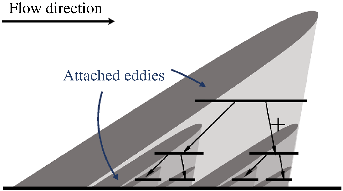
Townsend (Reference Townsend1976) proposed to model high Reynolds number boundary layers as collections of self-similar, wall-attached eddies (see figure 1). The velocity fluctuation at a generic point in the flow field can be computed by adding all the eddy-induced velocities at that point. The model therefore provides a method for calculating flow statistics based on randomly distributed wall-attached eddies (Perry & Chong Reference Perry and Chong1982; Marušic & Perry Reference Marušic and Perry1995; Perry & Marušic Reference Perry and Marušic1995) using the Biot–Savart law. The HRAP model models the induced velocities as random addends. The longitudinal velocity fluctuation is modelled as
 $$\begin{eqnarray}u=\mathop{\sum }_{i=1}^{N_{z}}a_{i},\end{eqnarray}$$
where a random addend
 $a_{i}$
is the velocity increment in
 $u$
due to an attached eddy of height
 ${\sim}\unicode[STIX]{x1D6FF}/2^{i}$
and the number of addends equals approximately
 $$\begin{eqnarray}N_{z}=\int _{z}^{\unicode[STIX]{x1D6FF}}P(z)\,\text{d}z\sim \log (\unicode[STIX]{x1D6FF}/z),\end{eqnarray}$$
where
 $P(z)=1/z$
is the eddy population density (see also figure 1). By relating
 $a_{i}$
to an attached eddy of height
 $\unicode[STIX]{x1D6FF}/2^{i}$
, we have discretized the boundary layer logarithmically in the wall-normal direction. Following Perry & Chong (Reference Perry and Chong1982) and also for convenience, the base 2 is used.
A schematic of the modelled boundary layer. The attached eddies are space filling. On a vertical plane cut as shown here, the number of eddies doubles as the size halves. An eddy affects the shaded region below it. The velocity at a generic point in the flow field is a result of the additive superposition of all the eddy-induced velocity fields there.

Following Townsend, inter-scale interactions are neglected in the HRAP formalism and the random addends,
 $a_{i}$
and
 $a_{j}$
, are statistically independent as long as
 $i\neq j$
. Neglecting the inter-scale interactions, i.e. amplitude and frequency modulation, is warranted as long as we restrict the discussion to the log region and quantities of interest to even-order statistics (Mathis et al.
Reference Mathis, Hutchins and Marusic2009; Mathis, Hutchins & Marusic Reference Mathis, Hutchins and Marusic2011). In addition to being statistically independent, the addends in (2.1) are statistically identical because the attached eddies are self-similar (according to the AEH).
Equation (2.1) along with the hierarchical eddy distribution as sketched in figure 1 can be used to derive the scalings in (1.2)–(1.7) (see Yang et al.
Reference Yang, Marusic and Meneveau2016a
,Reference Yang, Marusic and Meneveau
b
). For example, here, we compute
 $\langle u^{2}\rangle$
. Squaring both sides of (2.1) leads to
 $$\begin{eqnarray}\langle u^{2}\rangle =N_{z}\langle a^{2}\rangle =A_{1,u}\log (\unicode[STIX]{x1D6FF}/z)+B_{1,u},\end{eqnarray}$$
thus recovering the logarithmic scaling of
 $\langle u^{2}\rangle$
as a function of the wall-normal distance, where
 $A_{1,u}$
and
 $B_{1,u}$
are constants and
 $a$
is a random addend and is equal to
 $a_{i}$
statistically.
Because attached eddies that carry momentum carry also passive scalars, we expect that the same HRAP formalism may also be used to model the kinematics of scalar fluctuations
 $$\begin{eqnarray}\unicode[STIX]{x1D703}=\mathop{\sum }_{i=1}^{N_{z}}b_{i},\end{eqnarray}$$
where
 $b_{i}$
are also identically independently distributed random addends (but probably with a different statistical distribution than the addends
 $a_{i}$
). Note also that by assuming the
 $b_{i}$
are identically independently distributed, we have limited ourselves to scales in the log region. Again, we consider only fluctuations and
 $\unicode[STIX]{x1D703}$
is the fluctuation of the passive scalar. The modelling approach here is similar to that in Perry & Chong (Reference Perry and Chong1982), except in Perry & Chong (Reference Perry and Chong1982) a specific shaped eddy is used and here we are using a more abstract representation. Having made this analogy, we anticipate the scalar counterparts of the logarithmic scalings in (1.2) to (1.7), whose expressions are obtained simply by replacing the longitudinal velocity fluctuation
 $u$
with the scalar fluctuation
 $\unicode[STIX]{x1D703}$
. In additional, because passive scalars are transported by the same eddies that carry the momentum, we can expect that
 $a_{i}$
and
 $b_{i}$
, which are addends due to the same attached eddy, are highly correlated. Hence we also consider a set of mixed scalings. First, we consider
 $\langle u\unicode[STIX]{x1D703}\rangle$
. According to the HRAP, we would have
 $$\begin{eqnarray}\langle u\unicode[STIX]{x1D703}\rangle =\mathop{\sum }_{i=1}^{N_{z}}\langle a_{i}b_{i}\rangle \sim \langle ab\rangle \log \left(\frac{\unicode[STIX]{x1D6FF}}{z}\right).\end{eqnarray}$$
A direct consequence of (2.5) is that the correlation coefficient
 $$\begin{eqnarray}R_{u\unicode[STIX]{x1D703}}=\frac{\langle u\unicode[STIX]{x1D703}\rangle }{\sqrt{\langle u^{2}\rangle \langle \unicode[STIX]{x1D703}^{2}\rangle }}=\frac{A_{1,u\unicode[STIX]{x1D703}}\log (\unicode[STIX]{x1D6FF}/z)+B_{1,u\unicode[STIX]{x1D703}}}{\sqrt{(A_{1,u}\log (\unicode[STIX]{x1D6FF}/z)+B_{1,u})(A_{1,\unicode[STIX]{x1D703}}\log (\unicode[STIX]{x1D6FF}/z)+B_{1,\unicode[STIX]{x1D703}})}}\approx \frac{A_{1,u\unicode[STIX]{x1D703}}}{\sqrt{A_{1,u}A_{1,\unicode[STIX]{x1D703}}}}\end{eqnarray}$$
is approximately constant in the logarithmic region (
 $z/\unicode[STIX]{x1D6FF}\rightarrow 0,z^{+}\gg 1,Re_{\unicode[STIX]{x1D70F}}\rightarrow \infty$
, where
 $+$
indicates normalization by wall units) at high Reynolds numbers, where
 $A_{1,\unicode[STIX]{x1D703}}$
,
 $B_{1,\unicode[STIX]{x1D703}}$
are the slope and the additive constant in the logarithmic scaling of
 $\langle \unicode[STIX]{x1D703}^{2}\rangle$
, and
 $A_{1,u\unicode[STIX]{x1D703}}$
,
 $B_{1,u\unicode[STIX]{x1D703}}$
are the slope and the additive constant in the logarithmic scaling of
 $\langle u\unicode[STIX]{x1D703}\rangle$
. Meneveau & Marusic (Reference Meneveau and Marusic2013) invoked the central limit theorem and assumed that
 $u^{2}$
, being a sum of many random variables, follows a Gaussian distribution. Here, (2.5) leads to the first set of mixed logarithmic scalings
 $$\begin{eqnarray}\langle (u\unicode[STIX]{x1D703})^{p}\rangle ^{1/p}\sim \log \left(\frac{\unicode[STIX]{x1D6FF}}{z}\right),\end{eqnarray}$$
because
 $u\unicode[STIX]{x1D703}$
is also a sum of random addends (i.e.
 $a_{i}b_{i}$
). The second and third sets of scalings (the
 $\log (r_{x}/z)$
and
 $\log (\unicode[STIX]{x1D6FF}/r)$
scalings) will involve two points that are separated by a distance
 $r_{x}$
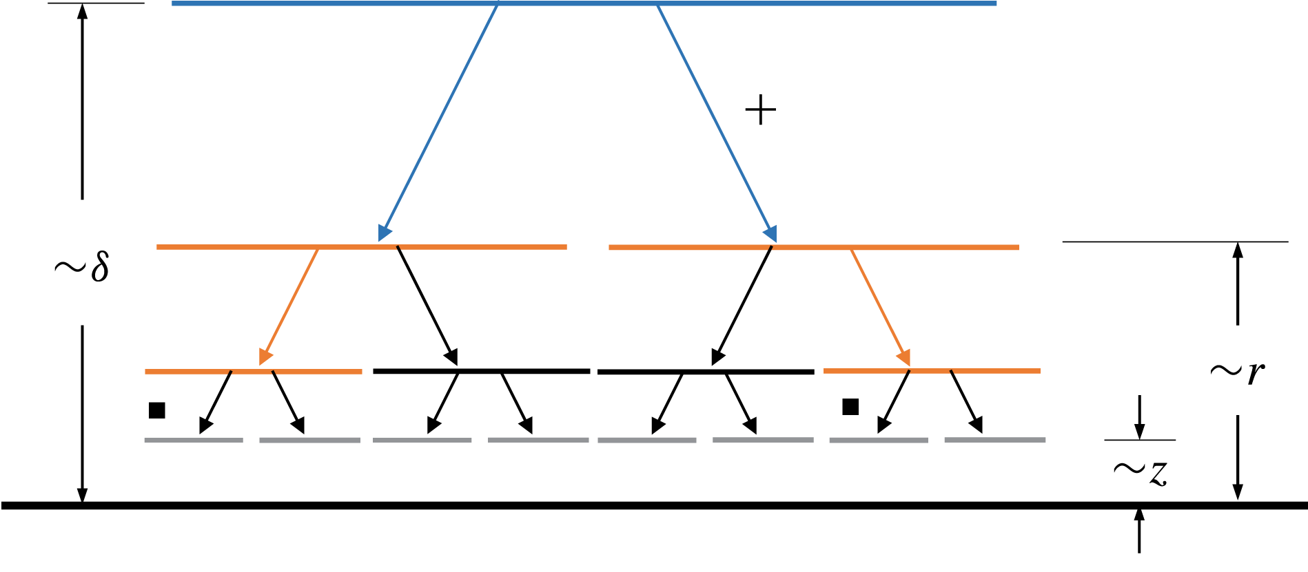
in the streamwise direction. Depending on the two-point distance, the attached eddies may be categorized into three types: first, eddies that affect simultaneously the two points (heights ranging from
 $\unicode[STIX]{x1D6FF}$
to
 ${\sim}r$
), which we will refer to as type-I eddies; second, eddies that affect either but not both of the two points (heights between
 ${\sim}r$
to
 ${\sim}z$
), which we will refer to as type-II eddies; third, eddies that affect neither of the two points (heights below
 ${\sim}z$
). In figure 2, we have sketched the three types of eddies. We consider
 $u(x)-u(x+r)$
and
 $\unicode[STIX]{x1D703}(x)-\unicode[STIX]{x1D703}(x+r)$
. Addends from type-I eddies cancel. Therefore both
 $u(x)-u(x+r)$
and
 $\unicode[STIX]{x1D703}(x)-\unicode[STIX]{x1D703}(x+r)$
account only for the addends from type-II eddies,
 $$\begin{eqnarray}u(x)-u(x+r)=\mathop{\sum }_{i=N_{z_{r}}}^{N_{z}}a_{i},\end{eqnarray}$$
where
 $z_{r}\sim r$
is the height of an attached eddy that extends
 $r$
in the streamwise direction. As we have discussed, addends with indices from
 $1$
to
 ${\sim}N_{z_{r}}$
are due to type-I eddies and they cancel. The second set of mixed scalings is
 $$\begin{eqnarray}\langle [(u(x)-u(x+r))(\unicode[STIX]{x1D703}(x)-\unicode[STIX]{x1D703}(x+r))]^{p}\rangle ^{1/p}=\langle ab\rangle (N_{z}-N_{z_{r}})\sim \log (r/z).\end{eqnarray}$$
Because
 $(u(x)-u(x+r))(\unicode[STIX]{x1D703}(x)-\unicode[STIX]{x1D703}(x+r))=\sum _{i=N_{z}}^{N_{z_{r}}}a_{i}b_{i}$
is also a sum of many random addends, following the same arguments that lead to the scalings in (2.7), the scalings in (2.9) can be easily obtained. Similarly, it follows that the third set of mixed logarithmic scalings is
 $$\begin{eqnarray}\displaystyle & \displaystyle \frac{1}{2}\left[\langle \unicode[STIX]{x1D703}(x)u(x+r_{x})\rangle +\langle u(x)\unicode[STIX]{x1D703}(x+r_{x})\rangle \right]\sim \log \frac{\unicode[STIX]{x1D6FF}}{r_{x}}, & \displaystyle\end{eqnarray}$$
 $$\begin{eqnarray}\displaystyle & \displaystyle \frac{3}{4}\left[\langle \unicode[STIX]{x1D703}^{2}(x)u^{2}(x+r_{x})\rangle +\langle u^{2}(x)\unicode[STIX]{x1D703}^{2}(x+r_{x})\rangle \right]-\frac{1}{2}\langle \unicode[STIX]{x1D703}^{2}u^{2}\rangle \sim \log \frac{\unicode[STIX]{x1D6FF}}{r_{x}}, & \displaystyle\end{eqnarray}$$
 $$\begin{eqnarray}\displaystyle & & \displaystyle \displaystyle \frac{5}{4}\left[\langle \unicode[STIX]{x1D703}^{3}(x)u^{3}(x+r_{x})\rangle +\langle u^{3}(x)\unicode[STIX]{x1D703}^{3}(x+r_{x})\rangle \right]\nonumber\\ \displaystyle & & \displaystyle \quad \displaystyle -\,\frac{3}{4}\left[\langle \unicode[STIX]{x1D703}(x)u^{5}(x+r_{x})\rangle +\langle u(x)\unicode[STIX]{x1D703}^{5}(x+r_{x})\rangle \right]\sim \log \frac{\unicode[STIX]{x1D6FF}}{r_{x}},\end{eqnarray}$$
The two points of interest are indicated using two black dots. The additive hierarchy in figure 1 is retained and we have removed the sketches for the attached eddies for brevity. For the particular two points under consideration, eddies in blue affect the two points simultaneously, eddies in orange can only affect one of the two points and eddies in grey affect neither of them.

where only addends of type-I attached eddies are retained. By swapping
 $\unicode[STIX]{x1D703}$
and
 $u$
at
 $x$
and
 $x+r$
(i.e. the use of
 $\left[\langle \unicode[STIX]{x1D703}(x)u(x+r_{x})\rangle +\langle u(x)\unicode[STIX]{x1D703}(x+r_{x})\rangle \right]$
instead of just
 $\langle \unicode[STIX]{x1D703}(x)u(x+r_{x})\rangle$
or
 $\langle u(x)\unicode[STIX]{x1D703}(x+r_{x})\rangle$
in (2.10)–(2.12)), we have accounted for possible asymmetry in the flow direction (private communication Y. Luo, 2017, Peking University), where the asymmetry refers to the fact that
 $\langle u^{m}(x+r)u^{n}(x)\rangle$
is not necessarily equal to
 $\langle u^{m}(x)u^{n}(x+r)\rangle$
. Likewise, accounting for the asymmetry in the flow direction, the scalings in (1.6) maybe rewritten as follows
 $$\begin{eqnarray}\displaystyle & \displaystyle \frac{1}{2}\left[\langle u(x)u(x+r_{x})\rangle +\langle u(x)u(x-r_{x})\rangle \right]\sim \log \frac{\unicode[STIX]{x1D6FF}}{r_{x}}, & \displaystyle\end{eqnarray}$$
 $$\begin{eqnarray}\displaystyle & \displaystyle \frac{3}{4}\left[\langle u^{2}(x)u^{2}(x+r_{x})\rangle +\langle u^{2}(x)u^{2}(x-r_{x})\rangle \right]-\frac{1}{2}\langle u^{4}\rangle \sim \log \frac{\unicode[STIX]{x1D6FF}}{r_{x}}, & \displaystyle\end{eqnarray}$$
 $$\begin{eqnarray}\displaystyle & \displaystyle \frac{5}{4}\langle u^{3}(x)(u^{3}(x+r_{x})+u^{3}(x-r_{x}))\rangle -\frac{3}{4}\langle u(x)(u^{5}(x+r_{x})+u^{5}(x+r_{x}))\rangle \sim \log \frac{\unicode[STIX]{x1D6FF}}{r_{x}}, & \displaystyle \nonumber\\ \displaystyle & & \displaystyle\end{eqnarray}$$
where correlations both in the positive
 $x$
direction and the negative
 $x$
direction are included. The scalar counterpart of (2.13)–(2.15) is straightforward, where one replaces
 $u$
with
 $\unicode[STIX]{x1D703}$
. According to the HRAP, the slopes of the logarithmic scalings of the second-order structure functions and the second-order two-point correlations are the same and equal the slope of the logarithmic scaling of their second-order single-point moment. Hence, the scalar/velocity correlation can also be defined for the second-order structure function and the second-order two-point correlations, and the HRAP predictions at high Reynolds numbers are
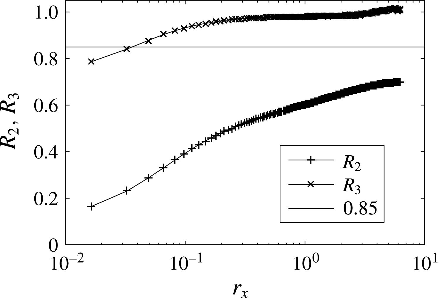
 $$\begin{eqnarray}\displaystyle & \displaystyle R_{2}=\frac{\langle DuD\unicode[STIX]{x1D703}\rangle }{\sqrt{\langle Du^{2}\rangle \langle D\unicode[STIX]{x1D703}^{2}\rangle }}\approx \frac{A_{1,u\unicode[STIX]{x1D703}}}{\sqrt{A_{1,u}A_{1,\unicode[STIX]{x1D703}}}}, & \displaystyle\end{eqnarray}$$
 $$\begin{eqnarray}\displaystyle & \displaystyle R_{3}=\frac{[\langle u(x)\unicode[STIX]{x1D703}(x+r_{x})\rangle +\langle \unicode[STIX]{x1D703}(x)u(x+r_{x})\rangle ]}{\sqrt{[\langle u(x)(u(x+r_{x})+u(x-r_{x}))\rangle ][\langle \unicode[STIX]{x1D703}(x)(\unicode[STIX]{x1D703}(x+r)+\unicode[STIX]{x1D703}(x-r_{x}))\rangle ]}}\approx \frac{A_{1,u\unicode[STIX]{x1D703}}}{\sqrt{A_{1,u}A_{1,\unicode[STIX]{x1D703}}}}, & \displaystyle \nonumber\\ \displaystyle & & \displaystyle\end{eqnarray}$$
i.e. independent of the wall-normal distance in the log region. Here
 $D\unicode[STIX]{x1D719}=\unicode[STIX]{x1D719}(x+r)-\unicode[STIX]{x1D719}(x)$
, and
 $\unicode[STIX]{x1D719}$
is
 $u$
or
 $\unicode[STIX]{x1D703}$
. Last, it is worth noting that the usefulness of the modelling framework developed here does not depend critically on the molecular Prandtl number (at least for
 $Pr\gtrsim 0.5$
) (see discussion in § 18.1.6 of Schlichting & Gersten Reference Schlichting and Gersten1999).
3 Large-eddy simulation framework
At high Reynolds numbers, the fluctuations of the passive scalars are dominated by the large-scale, momentum-carrying and energy-containing eddies. LES resolves the turbulent structures larger than a certain size, while the contribution of the unresolved small-scale eddies is parametrized. Hence it is the ideal tool for testing the modelling framework developed in the previous section.
3.1 LES governing equations
The LES framework used in this study is based on the filtered incompressible Navier–Stokes equations as well as the transport equation for the scalar concentration without any source term (i.e.
 $S=0$
in (1.1)):
 $$\begin{eqnarray}\unicode[STIX]{x2202}_{i}\widetilde{U}_{i}=0,\quad \unicode[STIX]{x2202}_{t}\widetilde{U}_{i}+\unicode[STIX]{x2202}_{j}(\widetilde{U}_{i}\widetilde{U}_{j})=-\frac{1}{\unicode[STIX]{x1D70C}}\unicode[STIX]{x2202}_{i}\widetilde{P}+\unicode[STIX]{x2202}_{j}(\unicode[STIX]{x1D708}\unicode[STIX]{x2202}_{j}\widetilde{U}_{i})-\unicode[STIX]{x2202}_{j}\unicode[STIX]{x1D70F}_{ij}\end{eqnarray}$$
and
 $$\begin{eqnarray}\unicode[STIX]{x2202}_{t}\widetilde{\unicode[STIX]{x1D6E9}}+\unicode[STIX]{x2202}_{i}(\widetilde{U}_{i}\widetilde{\unicode[STIX]{x1D6E9}})=\unicode[STIX]{x2202}_{i}({\mathcal{D}}\unicode[STIX]{x2202}_{i}\widetilde{\unicode[STIX]{x1D6E9}})-\unicode[STIX]{x2202}_{i}q_{i},\end{eqnarray}$$
where the tilde denotes spatial filtering,
 $\widetilde{U}_{i}$
and
 $\widetilde{\unicode[STIX]{x1D6E9}}$
are the resolved velocity and scalar concentration, respectively,
 $\widetilde{P}$
is the filtered pressure,
 $\unicode[STIX]{x1D70C}$
and
 $\unicode[STIX]{x1D708}$
are the fluid density and molecular viscosity, respectively,
 $\unicode[STIX]{x1D70F}_{ij}=\widetilde{U_{i}U_{j}}-\widetilde{U}_{i}\widetilde{U}_{j}$
is the SGS stress tensor, and
 $q_{i}=\widetilde{U_{i}\unicode[STIX]{x1D6E9}}-\widetilde{U}_{i}\widetilde{\unicode[STIX]{x1D6E9}}$
is the SGS scalar flux. For convenience, we will use
 $\unicode[STIX]{x1D6E9}$
alternatively as the resolved scalar concentration.
3.2 Subgrid-scale (SGS) parametrization
A common parametrization strategy in LES consists of computing the deviatoric part of the SGS stress with an eddy-viscosity model (Smagorinsky Reference Smagorinsky1963):
 $$\begin{eqnarray}\unicode[STIX]{x1D70F}_{ij}^{d}=\unicode[STIX]{x1D70F}_{ij}-{\textstyle \frac{1}{3}}\unicode[STIX]{x1D6FF}_{ij}\unicode[STIX]{x1D70F}_{kk}=-2\widetilde{\unicode[STIX]{x1D6E5}}^{2}C_{S}^{2}|\widetilde{\unicode[STIX]{x1D61A}}|\widetilde{\unicode[STIX]{x1D61A}}_{ij},\end{eqnarray}$$
and the SGS scalar flux with an eddy-diffusivity model:
 $$\begin{eqnarray}q_{i}=-\widetilde{\unicode[STIX]{x1D6E5}}^{2}C_{S}^{2}Sc_{sgs}^{-1}|\widetilde{\unicode[STIX]{x1D61A}}|\unicode[STIX]{x2202}_{i}\widetilde{\unicode[STIX]{x1D6E9}},\end{eqnarray}$$
where
 $\widetilde{\unicode[STIX]{x1D61A}}_{ij}=(\unicode[STIX]{x2202}_{i}\widetilde{U}_{j}+\unicode[STIX]{x2202}_{j}\widetilde{U}_{i})/2$
is the resolved strain-rate tensor whose magnitude is
 $|\widetilde{\unicode[STIX]{x1D61A}}|$
,
 $\widetilde{\unicode[STIX]{x1D6E5}}$
is the filter width,
 $C_{S}$
is the Smagorinsky coefficient,
 $C_{S}^{2}Sc_{sgs}^{-1}$
is the lumped coefficient and
 $Sc_{sgs}$
is the SGS Schmidt number. Here, the scale-dependent Lagrangian dynamic model (Bou-Zeid et al.
Reference Bou-Zeid, Meneveau and Parlange2005; Stoll & Porté-Agel Reference Stoll and Porté-Agel2006) is employed to compute the local optimized value of the model coefficients without any ad hoc tuning. In contrast with the traditional dynamic models (Germano et al.
Reference Germano, Piomelli, Moin and Cabot1991; Moin, Squires & Lee Reference Moin, Squires and Lee1991), the scale-dependent dynamic models compute dynamically not only the value of the model coefficients in the eddy-viscosity and eddy-diffusivity models, but also the dependence of these coefficients with scale. More details on the formulation of the scale-dependent Lagrangian dynamic models for the SGS turbulent fluxes can be found in Bou-Zeid et al. (Reference Bou-Zeid, Meneveau and Parlange2005) and Stoll & Porté-Agel (Reference Stoll and Porté-Agel2006).
3.3 Numerical set-up
The computational domain is discretized uniformly into
 $N_{x}\times N_{y}\times N_{z}$
grid points with a spatial resolution of
 $\unicode[STIX]{x1D6E5}_{x}\times \unicode[STIX]{x1D6E5}_{y}\times \unicode[STIX]{x1D6E5}_{z}$
in the streamwise, spanwise and wall-normal directions, respectively. The grid planes are staggered in the vertical direction, with the first vertical velocity plane at a distance
 $\unicode[STIX]{x1D6E5}_{z}$
from the surface, and the first horizontal velocity plane
 $\unicode[STIX]{x1D6E5}_{z}/2$
from the surface. The size of the computational domain is
 $4\unicode[STIX]{x03C0}\unicode[STIX]{x1D6FF}\times 2\unicode[STIX]{x03C0}\unicode[STIX]{x1D6FF}\times \unicode[STIX]{x1D6FF}$
, where
 $\unicode[STIX]{x1D6FF}$
is the half channel height. In this study, two different spatial resolutions are used to test the resolution sensitivity of the simulation results (see § 4 for details). The code uses a pseudo-spectral discretization in the wall-parallel directions and a second-order central finite difference scheme in the wall-normal direction (Albertson & Parlange Reference Albertson and Parlange1999; Porté-Agel, Meneveau & Parlange Reference Porté-Agel, Meneveau and Parlange2000; Porté-Agel Reference Porté-Agel2004). The equations are integrated in time using a second-order accurate Adams–Bashforth scheme. Since the Reynolds number is high, no near-wall viscous processes are resolved, and the viscous terms are neglected in the governing equations. In the streamwise and spanwise directions, periodic boundary conditions are applied for both the velocity and the scalar fields. The upper boundary conditions are a zero-stress zero-flux condition and zero vertical velocity, i.e.
 $\unicode[STIX]{x2202}\widetilde{U}/\unicode[STIX]{x2202}z=0$
,
 $\unicode[STIX]{x2202}\widetilde{V}/\unicode[STIX]{x2202}z=0$
,
 $\widetilde{W}=0$
,
 $\unicode[STIX]{x2202}\widetilde{\unicode[STIX]{x1D6E9}}/\unicode[STIX]{x2202}z=0$
.
3.4 Wall modelling
If all the scales were resolved, the wall boundary condition is a no-slip condition for the velocities and a constant scalar flux condition for the passive scalar. In a wall-modelled calculation, because the near-wall fluid flows are not resolved, the no-slip boundary condition cannot be used directly and the typical practice is to replace the no slip (Dirichlet-type boundary condition) with a stress boundary condition (Neumann-type boundary condition), which provides the necessary flux at the wall for integrating the momentum equation (see e.g. Piomelli & Balaras Reference Piomelli and Balaras2002; Choi & Moin Reference Choi and Moin2012). The wall shear stress is specified as a Neumann boundary condition according to a wall model (Bou-Zeid, Meneveau & Parlange Reference Bou-Zeid, Meneveau and Parlange2004)
 $$\begin{eqnarray}\displaystyle & \displaystyle \unicode[STIX]{x1D70F}_{xz}|_{w}(x,y)=\left[\frac{\unicode[STIX]{x1D705}U_{||}}{\log (h_{wm}/z_{o})}\right]^{2}\frac{U_{wm}(x,y)}{U_{||}}, & \displaystyle\end{eqnarray}$$
 $$\begin{eqnarray}\displaystyle & \displaystyle \unicode[STIX]{x1D70F}_{yz}|_{w}(x,y)=\left[\frac{\unicode[STIX]{x1D705}U_{||}}{\log (h_{wm}/z_{o})}\right]^{2}\frac{V_{wm}(x,y)}{U_{||}}, & \displaystyle\end{eqnarray}$$
where
 $\unicode[STIX]{x1D70F}|_{w}$
is the wall shear stress and
 $\unicode[STIX]{x1D705}\approx 0.4$
is the von Kármán constant,
 $h_{wm}=\unicode[STIX]{x1D6E5}_{z}/2$
is the distance of the first LES grid point from the wall,
 $z_{o}$
is the viscous/roughness length scale (for a smooth wall,
 $z_{o}=\exp (-\unicode[STIX]{x1D705}B)\unicode[STIX]{x1D708}/u_{\unicode[STIX]{x1D70F}}$
, where
 $B$
is the additive constant in the incompressible law of the wall),
 $U_{||}=\sqrt{U_{wm}^{2}(x,y)+V_{wm}^{2}(x,y)}$
is the wall-parallel velocity at the first level
 $\unicode[STIX]{x1D6E5}_{z}/2$
,
 $U_{wm}(x,y)$
and
 $V_{wm}(x,y)$
are the spatially filtered LES velocities in the streamwise and spanwise directions at that same height (Bou-Zeid et al.
Reference Bou-Zeid, Meneveau and Parlange2005; Yang, Park & Moin Reference Yang, Park and Moin2017b
), i.e.
 $$\begin{eqnarray}U_{wm}(x,y)=\hat{\widetilde{U}}(x,y,z=\unicode[STIX]{x1D6E5}_{z}/2),\quad \text{and}\quad V_{wm}(x,y)=\hat{\widetilde{V}}(x,y,z=\unicode[STIX]{x1D6E5}_{z}/2),\end{eqnarray}$$
where
 $\hat{\cdot }$
is a low-pass filtering in the Fourier space that cuts off at wavenumbers
 $k_{x}=\unicode[STIX]{x03C0}/(2\unicode[STIX]{x1D6E5}_{x})$
and
 $k_{y}=\unicode[STIX]{x03C0}/(2\unicode[STIX]{x1D6E5}_{y})$
. This filtering is not fixed in physical space, but is commensurate with the grid. The boundary layer is driven by an imposed uniform pressure gradient
 $-\unicode[STIX]{x1D70C}u_{\unicode[STIX]{x1D70F}}^{2}/\unicode[STIX]{x1D6FF}$
in the streamwise direction, where
 $u_{\unicode[STIX]{x1D70F}}$
is the friction velocity. The surface viscous/roughness scale
 $z_{o}/\unicode[STIX]{x1D6FF}$
is set to
 $1.0\times 10^{-5}$
, which corresponds to a smooth channel flow at
 $Re_{\unicode[STIX]{x1D70F}}=1.4\times 10^{4}$
.
In practice, the computed wall shear stresses are used in a Neumann boundary condition
 $$\begin{eqnarray}\left[\left(\unicode[STIX]{x1D708}_{t}+\unicode[STIX]{x1D708}\right)\frac{\unicode[STIX]{x2202}\widetilde{U}}{\unicode[STIX]{x2202}z}\right]_{z=0}=\unicode[STIX]{x1D70F}_{xz}|_{w},\quad \left[\left(\unicode[STIX]{x1D708}_{t}+\unicode[STIX]{x1D708}\right)\frac{\unicode[STIX]{x2202}\widetilde{V}}{\unicode[STIX]{x2202}z}\right]_{z=0}=\unicode[STIX]{x1D70F}_{yz}|_{w}.\end{eqnarray}$$
The wall-normal velocity gradients
 $\unicode[STIX]{x2202}\widetilde{U}/\unicode[STIX]{x2202}z$
,
 $\unicode[STIX]{x2202}\widetilde{V}/\unicode[STIX]{x2202}z$
may be computed using (3.8), with the eddy viscosity at the wall specified according to
 $$\begin{eqnarray}\left.\unicode[STIX]{x1D708}_{t}\right|_{z=0}=\left.\unicode[STIX]{x1D708}_{t}\right|_{z=\unicode[STIX]{x1D6E5}_{z}/2}.\end{eqnarray}$$
 $z=\unicode[STIX]{x1D6E5}_{z}/2$
is the distance between the first off-wall grid point and the wall (because of the use of a staggered grid, it is
 $\unicode[STIX]{x1D6E5}_{z}/2$
instead of
 $\unicode[STIX]{x1D6E5}_{z}$
). The computed wall-normal velocity gradients then can be used for computing a velocity at
 $z=-\unicode[STIX]{x1D6E5}_{z}/2$
(below the wall, which is a ghost point),
 $$\begin{eqnarray}\displaystyle & \displaystyle \widetilde{U}(z=-\unicode[STIX]{x1D6E5}_{z}/2)=\widetilde{U}(z=\unicode[STIX]{x1D6E5}_{z}/2)-[\unicode[STIX]{x2202}\widetilde{U}/\unicode[STIX]{x2202}z]_{w}\cdot \unicode[STIX]{x1D6E5}_{z}, & \displaystyle\end{eqnarray}$$
 $$\begin{eqnarray}\displaystyle & \displaystyle \widetilde{V}(z=-\unicode[STIX]{x1D6E5}_{z}/2)=\widetilde{V}(z=\unicode[STIX]{x1D6E5}_{z}/2)-[\unicode[STIX]{x2202}\widetilde{V}/\unicode[STIX]{x2202}z]_{w}\cdot \unicode[STIX]{x1D6E5}_{z}. & \displaystyle\end{eqnarray}$$
Equations (3.8), (3.9), (3.11) provide the necessary Neumann boundary condition for the wall-parallel velocities. The boundary condition of the wall-normal velocity is
 $\widetilde{W}=0$
, i.e. no penetration.
At a statistically stationary state, the imposed pressure gradient is balanced by the wall shear stress (e.g. if the imposed pressure gradient is greater than the computed wall shear stresses, the flow accelerates, increasing
 $U_{wm}$
in (3.6), which in turn increases the wall shear stress in the flow direction, until a statistically stationary state is reached). Define
 $u_{\unicode[STIX]{x1D70F}}^{(1)}=\sqrt{-1/\unicode[STIX]{x1D70C}~\text{d}p_{\infty }/\text{d}x~\unicode[STIX]{x1D6FF}}$
to be the necessary friction velocity for balancing the imposed pressure gradient. Define also
 $u_{\unicode[STIX]{x1D70F}}^{(2)}(t)=\sqrt{\unicode[STIX]{x1D70F}_{w}(t)/\unicode[STIX]{x1D70C}}$
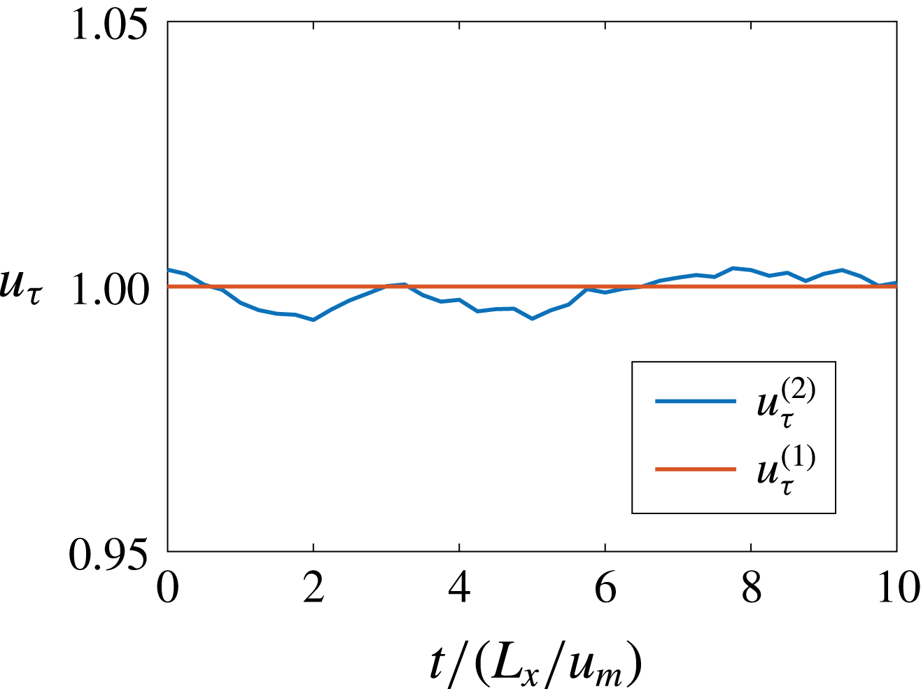
to be the friction velocity that corresponds to the plane-averaged skin friction. Figure 3 shows a sample time history of the two friction velocities after the flow reaches a statistically stationary state, and we can conclude that
 $\langle u_{\unicode[STIX]{x1D70F}}^{(1)}\rangle =\langle u_{\unicode[STIX]{x1D70F}}^{(2)}\rangle$
.
Sample time history of
 $u_{\unicode[STIX]{x1D70F}}^{(1)}$
and
 $u_{\unicode[STIX]{x1D70F}}^{(2)}$
after the flow has reached a statistically stationary state. Results from the fine grid calculation are presented.

The above reasoning for specifying boundary conditions for the velocity field applies equally to the scalar field. If one resolves all the scales (i.e. conducing a DNS), a scalar concentration may be imposed at the wall. Presently a Dirichlet-type boundary condition is replaced with a wall-modelled constant flux condition at the bottom wall. While this may produce non-physical scalar excursions in the sense of unbounded scalar values, it will be shown to give an approximately stationary scalar fluctuation field. This model is therefore adopted for the purposes of the present study. For simplicity and following previous works, a constant (both in space and in time) downward scalar flux
 $$\begin{eqnarray}q_{z}|_{w}=-u_{\unicode[STIX]{x1D70F}}\unicode[STIX]{x1D703}_{\unicode[STIX]{x1D70F}}\end{eqnarray}$$
is imposed at the wall similar to the one used in previous studies (Andren et al. Reference Andren, Brown, Mason, Graf, Schumann, Moeng and Nieuwstadt1994; Kong, Choi & Lee Reference Kong, Choi and Lee2000; Porté-Agel Reference Porté-Agel2004; Stoll & Porté-Agel Reference Stoll and Porté-Agel2006; Lu & Porté-Agel Reference Lu and Porté-Agel2013; Abkar, Bae & Moin Reference Abkar, Bae and Moin2016). The constant wall flux is imposed as a Neumann boundary condition
 $$\begin{eqnarray}\left[({\mathcal{D}}_{t}+{\mathcal{D}})\frac{\unicode[STIX]{x2202}\widetilde{\unicode[STIX]{x1D6E9}}}{\unicode[STIX]{x2202}z}\right]_{z=0}=\left.q_{z}\right|_{w},\end{eqnarray}$$
where the eddy diffusivity
 ${\mathcal{D}}_{t}$
at the wall is the same as its value at the first off-wall LES point
 $$\begin{eqnarray}\left.{\mathcal{D}}_{t}\right|_{w}=\left.{\mathcal{D}}_{t}\right|_{z=\unicode[STIX]{x1D6E5}_{z}/2}.\end{eqnarray}$$
The necessary Neumann boundary condition for
 $\unicode[STIX]{x2202}\widetilde{\unicode[STIX]{x1D6E9}}/\unicode[STIX]{x2202}z$
may be computed according to (3.13), which is then used for computing the concentration of the passive scalar at the ghost point
 $$\begin{eqnarray}\widetilde{\unicode[STIX]{x1D6E9}}(z=-\unicode[STIX]{x1D6E5}_{z}/2)=\widetilde{\unicode[STIX]{x1D6E9}}(z=\unicode[STIX]{x1D6E5}_{z}/2)-[\unicode[STIX]{x2202}\widetilde{\unicode[STIX]{x1D6E9}}/\unicode[STIX]{x2202}z]_{w}\cdot \unicode[STIX]{x1D6E5}_{z}.\end{eqnarray}$$
Equations (3.13), (3.14), (3.15) provide the necessary boundary conditions for the passive scalar. We have imposed
 $q_{z}|_{w}$
, which determines
 $\unicode[STIX]{x1D703}_{\unicode[STIX]{x1D70F}}$
, or one may impose
 $\unicode[STIX]{x1D703}_{\unicode[STIX]{x1D70F}}$
, which in turn determines the flux
 $q_{z}|_{w}$
. The quantity
 $\unicode[STIX]{x1D703}_{\unicode[STIX]{x1D70F}}$
introduced here is not directly used in the simulation but will be used for normalizing the computed flow quantities. While the near-wall small-scale eddies whose heights extends only a few grid points are affected by this boundary condition, the larger-scale eddies are mostly unaffected (see e.g. Yang et al.
Reference Yang, Park and Moin2017b
).
3.5 Properties of the scalar field
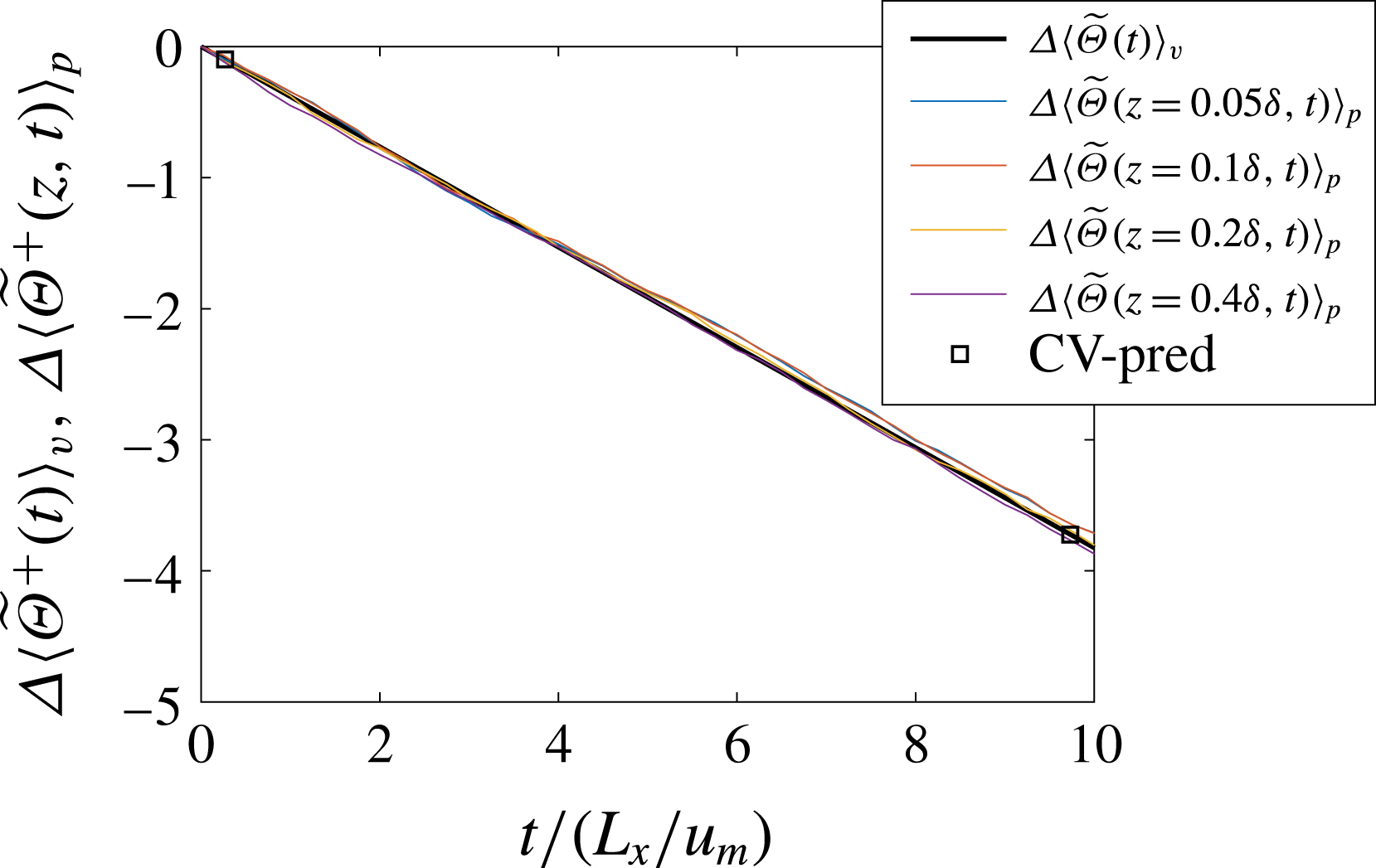
Since we impose a constant scalar flux at the bottom wall, the bulk scalar magnitude changes in time. Figure 4 shows a sample time history of the volume-averaged
 $\widetilde{\unicode[STIX]{x1D6E9}}$
(averaged in the three-dimensional space but not in time) and the plane-averaged
 $\widetilde{\unicode[STIX]{x1D6E9}}$
(averaged in the two homogeneous directions, but not in time nor in
 $z$
) as a function of time for 10 flow throughs. The volume-averaged and the plane-averaged scalar concentrations are denoted as
 $\langle \widetilde{\unicode[STIX]{x1D6E9}}(t)\rangle _{v}$
and
 $\langle \widetilde{\unicode[STIX]{x1D6E9}}(z,t)\rangle _{p}$
, with the subscripts
 $v$
and
 $p$
denoting ‘volume’ and ‘plane’. According to the conservation law, the volume-averaged scalar concentration
 $\langle \widetilde{\unicode[STIX]{x1D6E9}}(t)\rangle _{v}$
varies linearly as a function of time, at a rate
 $q_{z}|_{w}/\unicode[STIX]{x1D6FF}$
(which is negative here). This bears out in figure 4. In addition, the plane-averaged scalar concentration
 $\langle \widetilde{\unicode[STIX]{x1D6E9}}(z,t)\rangle _{p}$
decreases at the same rate. This is quite convenient because
 $$\begin{eqnarray}\frac{\text{d}\langle \widetilde{\unicode[STIX]{x1D6E9}}(z,t)\rangle _{p}}{\text{d}z}=\frac{\text{d}[\langle \widetilde{\unicode[STIX]{x1D6E9}}(z,t_{0})\rangle _{p}+(\left.q_{z}\right|_{w}/\unicode[STIX]{x1D6FF})\cdot t]}{\text{d}z}=\frac{\text{d}\langle \widetilde{\unicode[STIX]{x1D6E9}}(z,t_{0})\rangle _{p}}{\text{d}z}\end{eqnarray}$$
is time independent (
 $t_{0}$
is a given time instant), and therefore we do not have to worry about the time dependence of
 $\widetilde{\unicode[STIX]{x1D6E9}}$
when computing spatial derivatives. In figure 4, the scalar concentrations are normalized using wall units
 $\unicode[STIX]{x1D703}_{\unicode[STIX]{x1D70F}}$
and is indicated using a superscript
 $+$
, i.e.
 $\widetilde{\unicode[STIX]{x1D6E9}}^{+}=\widetilde{\unicode[STIX]{x1D6E9}}/\unicode[STIX]{x1D703}_{\unicode[STIX]{x1D70F}}$
.
 $\langle \widetilde{\unicode[STIX]{x1D6E9}}(t)\rangle _{v}$
and
 $\langle \widetilde{\unicode[STIX]{x1D6E9}}(z,t)\rangle _{p}$
for
 $z=0.05\unicode[STIX]{x1D6FF}$
,
 $0.1\unicode[STIX]{x1D6FF}$
,
 $0.2\unicode[STIX]{x1D6FF}$
,
 $0.4\unicode[STIX]{x1D6FF}$
as functions of the time. Normalizations are by
 $\unicode[STIX]{x1D703}_{\unicode[STIX]{x1D70F}}$
and
 $L_{x}/u_{m}$
.
 $\unicode[STIX]{x1D6E5}\langle \widetilde{\unicode[STIX]{x1D6E9}}(t)\rangle _{v}=\langle \widetilde{\unicode[STIX]{x1D6E9}}(t)\rangle _{v}-\langle \widetilde{\unicode[STIX]{x1D6E9}}(t=0)\rangle _{v}$
.
 $\langle \widetilde{\unicode[STIX]{x1D6E9}}(z,t)\rangle _{p}=\langle \widetilde{\unicode[STIX]{x1D6E9}}(z,t)\rangle _{p}-\langle \widetilde{\unicode[STIX]{x1D6E9}}(z,t=0)\rangle _{p}$
. The exact magnitude of the two quantities at
 $t=t_{0}$
is not relevant and we need only to focus on the change. ‘CV-pred’ is the expected rate at which the volume-averaged scalar concentration decreases (which is
 $q_{z}|_{w}/\unicode[STIX]{x1D6FF}$
), and the expected linear decrease is indicated using two squares (a line is specified using two points, and we are using two points instead of a line for better visualizations). Results from the fine grid calculation are presented.

While
 $\widetilde{\unicode[STIX]{x1D6E9}}(x,y,z,t)$
decreases with time, the scalar fluctuation
 $\unicode[STIX]{x1D703}$
is approximately statistically stationary after a few flow throughs. By definition, the scalar fluctuation is
 $\unicode[STIX]{x1D703}=\widetilde{\unicode[STIX]{x1D6E9}}(x,y,z,t)-\langle \widetilde{\unicode[STIX]{x1D6E9}}(x,y,z,t)\rangle$
.
 $\langle \cdot \rangle$
denotes ensemble average. For the quantity
 $\langle \widetilde{\unicode[STIX]{x1D6E9}}(x,y,z,t)\rangle$
, the ensemble average is approximated using an average in the streamwise and spanwise directions. Define
 $$\begin{eqnarray}r(z,t,p)=\langle \unicode[STIX]{x1D703}^{2p}(z,t)\rangle /\langle \unicode[STIX]{x1D703}^{2p}(z,t_{0})\rangle ,\end{eqnarray}$$
where the superscript
 $p=1,2,3,\ldots$
is an integer, and
 $\langle \cdot \rangle$
indicates a plane average,
 $t_{0}$
is a given (arbitrary) time instant,
 $t>t_{0}$
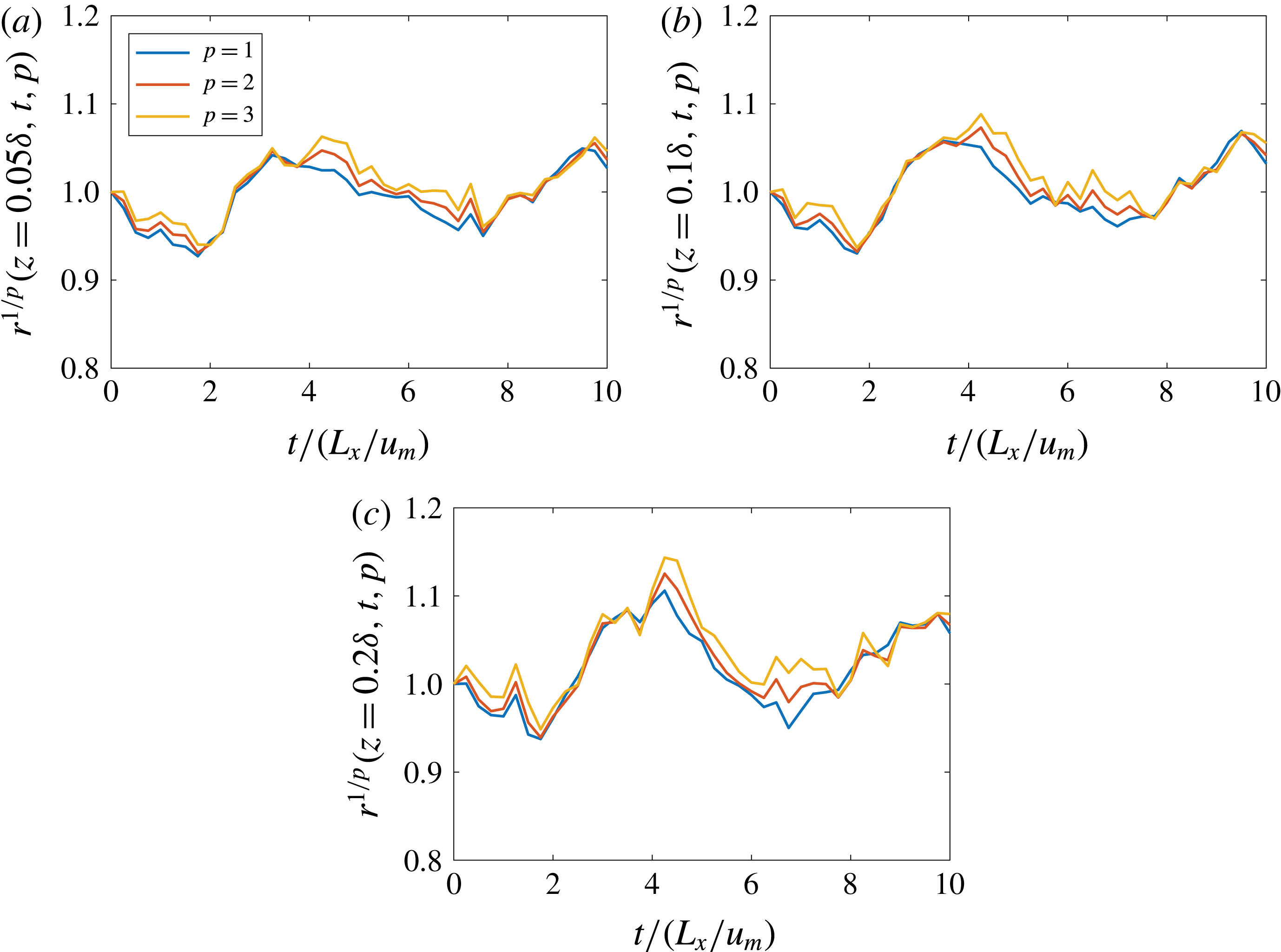
is the time. Figure 5 shows a few sample time histories of
 $r^{1/p}$
as functions of time for
 $z=0.05\unicode[STIX]{x1D6FF}$
,
 $0.1\unicode[STIX]{x1D6FF}$
,
 $0.2\unicode[STIX]{x1D6FF}$
and for
 $p=1,2,3$
. According to figure 5, the scalar fluctuation
 $\unicode[STIX]{x1D703}$
is statistically stationary to a good approximation within the considered period of time.
(a)
 $r^{1/p}$
at
 $z=0.05\unicode[STIX]{x1D6FF}$
as function of time for
 $p=1$
, 2, 3 for 10 flow throughs. (b) Same as (a) but for
 $z=0.1\unicode[STIX]{x1D6FF}$
. (c) Same as (a) but for
 $z=0.2\unicode[STIX]{x1D6FF}$
. Here the
 $1/p$
th power is taken for better visualization. According to the definition of
 $r$
in (3.17), the normalization is by
 $\langle \unicode[STIX]{x1D703}^{2p}(z,t_{0})\rangle$
, and therefore
 $r^{1/p}(z,t,p)$
does not necessarily fluctuate around 1, even if
 $\unicode[STIX]{x1D703}$
is statistically stationary (although for the figures here, they happen to fluctuate around 1). Results from the fine grid calculation are presented.

The actual magnitude of the surface scalar flux has no influence on the results presented here (Stoll & Porté-Agel Reference Stoll and Porté-Agel2006). All the statistics are averaged over 10 flow throughs after the flow reaches a statistical stationary state (one flow through is
 $t_{f}\approx L_{x}/u_{m}$
, where
 $u_{m}$
is the volume-averaged velocity). Worth noting here is the LES code has been well validated and used in various previous publications (see e.g. Porté-Agel et al.
Reference Porté-Agel, Meneveau and Parlange2000; Porté-Agel Reference Porté-Agel2004; Stoll & Porté-Agel Reference Stoll and Porté-Agel2006, Reference Stoll and Porté-Agel2009; Abkar & Porté-Agel Reference Abkar and Porté-Agel2012, Reference Abkar and Porté-Agel2014, Reference Abkar and Porté-Agel2015, Reference Abkar and Porté-Agel2016; Abkar et al.
Reference Abkar, Bae and Moin2016; Abkar & Moin Reference Abkar and Moin2017).
4 Grid convergence
In this section grid convergence for a few statistics of interest is tested. We consider two grids, which are of sizes
 $512\times 256\times 128$
and
 $768\times 384\times 192$
in the
 $x$
,
 $y$
,
 $z$
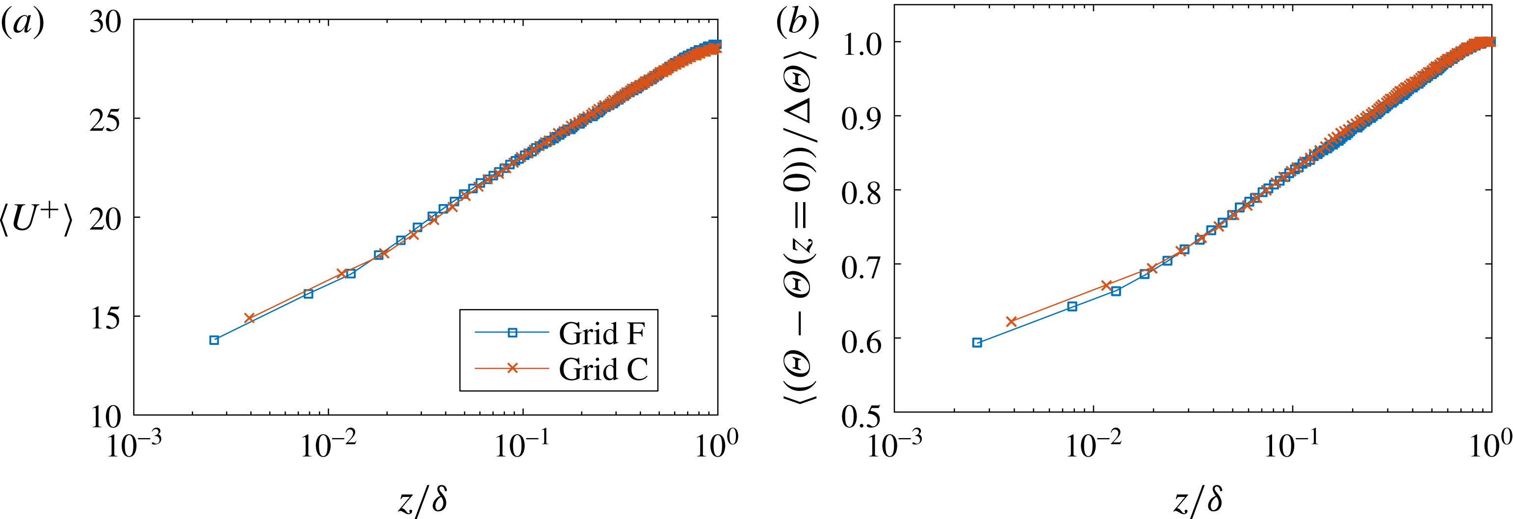
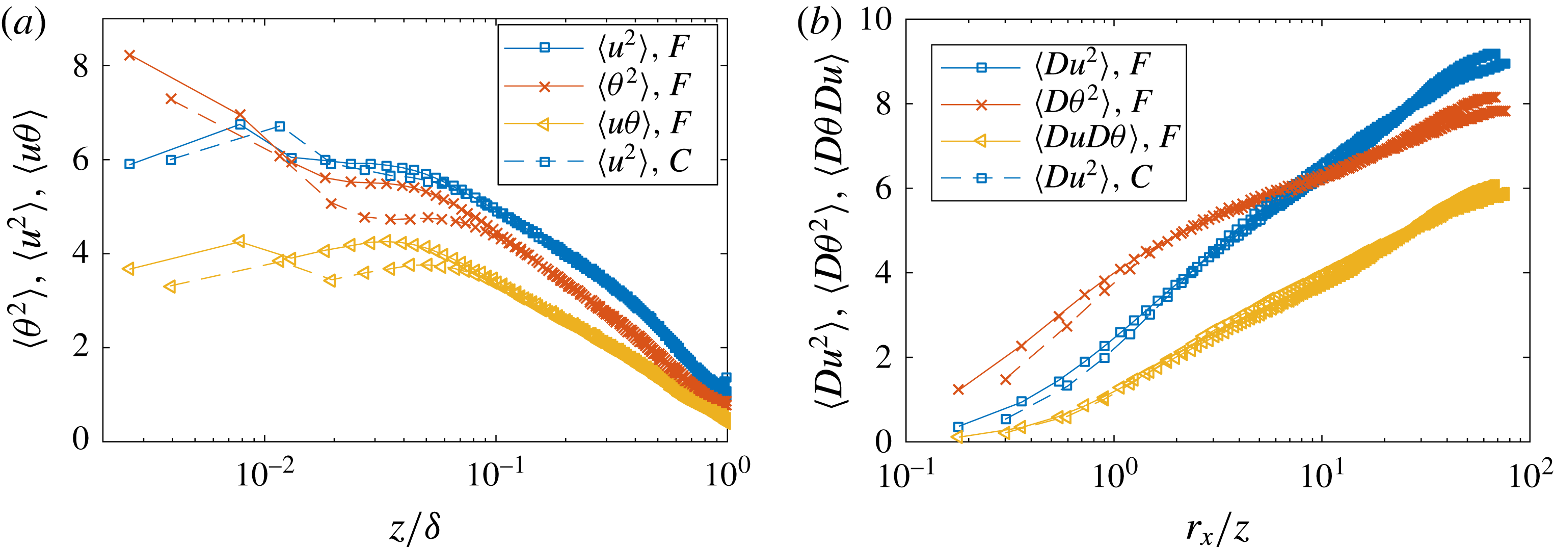
directions respectively. Figure 6 shows the mean velocity and the mean scalar concentration. Both the mean velocity field and the mean scalar concentration field are grid converged, although the solution at the first three off-wall grid points does not follow precisely the log law (Kawai & Larsson Reference Kawai and Larsson2012). In figure 7, we compare
 $\langle \unicode[STIX]{x1D703}^{2}\rangle$
,
 $\langle u^{2}\rangle$
,
 $\langle \unicode[STIX]{x1D703}u\rangle$
, as well as
 $\langle \unicode[STIX]{x0394}\unicode[STIX]{x1D703}^{2}\rangle$
,
 $\langle \unicode[STIX]{x0394}u^{2}\rangle$
,
 $\langle \unicode[STIX]{x0394}\unicode[STIX]{x1D703}\unicode[STIX]{x0394}u\rangle$
from the two LES. For the single-point second-order moments, convergence is only expected a few grid points (
 ${\approx}10$
) away from the wall (see detailed discussion in Yang et al. (Reference Yang, Park and Moin2017b
)), where the numerical solutions are less susceptible to numerical errors in the near-wall region. According to figure 7(a), approximately 10 grid points away from the wall, the statistics are grid converged, yielding the same logarithmic scalings and the same slopes for
 $\langle u^{2}\rangle$
,
 $\langle \unicode[STIX]{x1D703}^{2}\rangle$
and
 $\langle u\unicode[STIX]{x1D703}\rangle$
. Figure 7(b) shows the second-order structure functions. Reasonable grid convergence is found within the logarithmic range and the slope of the log scalings are no different between the two grids. Similar results are found for other statistics and are not shown here for brevity.
(a) Mean velocity as function of the wall-normal distance. ‘grid F’ denotes the fine grid and ‘grid C’ denotes the coarse grid. (b) Mean scalar concentration as function of the wall-normal distance.
 $\unicode[STIX]{x0394}\unicode[STIX]{x1D6E9}$
is the difference between the scalar concentrations at the top of the half-channel and at the bottom wall.

(a) Single-point second-order moments
 $\langle \unicode[STIX]{x1D703}^{2}\rangle$
,
 $\langle u^{2}\rangle$
,
 $\langle \unicode[STIX]{x1D703}u\rangle$
as functions of the wall-normal distance. (b) Second-order structure functions
 $\langle \unicode[STIX]{x0394}\unicode[STIX]{x1D703}^{2}\rangle$
,
 $\langle \unicode[STIX]{x0394}u^{2}\rangle$
,
 $\langle \unicode[STIX]{x0394}\unicode[STIX]{x1D703}\unicode[STIX]{x0394}u\rangle$
as functions of the two-point displacements at
 $z/\unicode[STIX]{x1D6FF}\approx 0.1$
. ‘F’ refers to the fine grid and ‘C’ refers to the coarse grid.

5 Results
We will test the HRAP model and show that LES, despite the modelling involved, captures as well the generalized scalings that were identified in experiments. First the code is validated. This is useful even though the code has been validated in previous works. Unless otherwise noted, both the longitudinal velocity and the scalar are normalized using wall units (
 $u_{\unicode[STIX]{x1D70F}}$
and
 $\unicode[STIX]{x1D703}_{\unicode[STIX]{x1D70F}}$
). Only results from the fine grid calculation are presented.
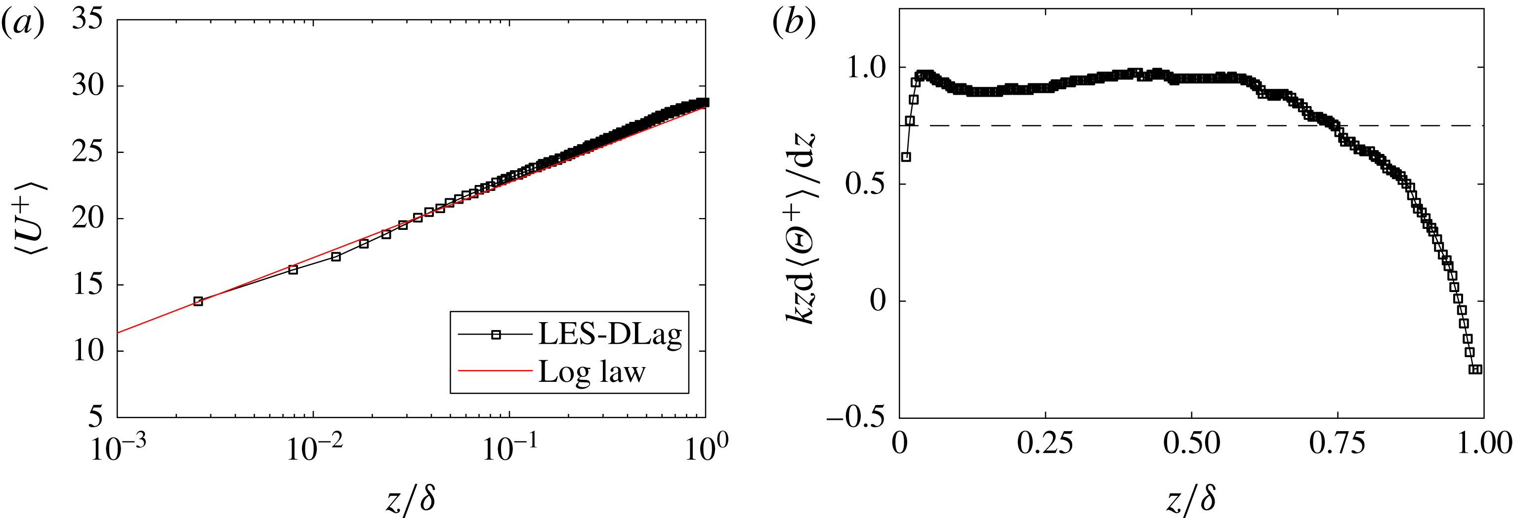
Figure 8 shows the mean velocity profile
 $\langle U^{+}\rangle$
and the profile of the mean scalar gradient
 $\unicode[STIX]{x1D705}z\text{d}\langle \unicode[STIX]{x1D6E9}^{+}\rangle /\text{d}z$
as functions of the wall-normal distance, where
 $\langle U\rangle$
is the mean velocity and
 $\langle \unicode[STIX]{x1D6E9}\rangle$
is the mean of the passive-scalar concentration. At any given instantaneous in time,
 $\langle \unicode[STIX]{x1D6E9}^{+}\rangle \sim \log (z/z_{o\unicode[STIX]{x1D703}})$
, where
 $z_{o\unicode[STIX]{x1D703}}$
is the equivalent roughness length scale for the scalar. One may compute
 $z_{o}$
according to the log law
 $$\begin{eqnarray}z_{o}=z\exp [-\unicode[STIX]{x1D705}(\langle U^{+}(z)\rangle -\langle U_{w}^{+}\rangle )],\end{eqnarray}$$
and one may also compute
 $z_{o\unicode[STIX]{x1D703}}$
according to the log law of the passive scalar
 $$\begin{eqnarray}z_{o\unicode[STIX]{x1D703}}=z\exp [-\unicode[STIX]{x1D705}_{\unicode[STIX]{x1D703}}(\langle \unicode[STIX]{x1D6E9}^{+}(z,t)\rangle -\langle \unicode[STIX]{x1D6E9}_{w}^{+}(t)\rangle )],\end{eqnarray}$$
where
 $\unicode[STIX]{x1D705}_{\unicode[STIX]{x1D703}}$
is the von Kármán constant of the scalar profile. Here,
 $U_{w}$
and
 $\unicode[STIX]{x1D6E9}_{w}$
are the velocity and the scalar concentration at the wall, respectively (note
 $U_{w}=0$
). It is also expected that
 $z\text{d}\langle \unicode[STIX]{x1D6E9}^{+}\rangle /\text{d}z\approx \text{Const.}$
in the log region. The mean velocity profile follows the log law closely and
 $z\text{d}\langle \unicode[STIX]{x1D6E9}^{+}\rangle /\text{d}z$
is approximately constant in the region
 $0.1<z/\unicode[STIX]{x1D6FF}<0.5$
, which is consistent with the reported trend in previous studies (Stoll & Porté-Agel Reference Stoll and Porté-Agel2006; Lu & Porté-Agel Reference Lu and Porté-Agel2013; Abkar et al.
Reference Abkar, Bae and Moin2016). Hence, the LES captures the behaviour of the first-order statistics.
(a) Mean velocity profile. The expected log law is
 $1/\unicode[STIX]{x1D705}\log (z/z_{o})$
, where
 $\unicode[STIX]{x1D705}\approx 0.4$
is the von Kármán constant and
 $z_{o}/\unicode[STIX]{x1D6FF}=10^{-5}$
is the effective roughness height. (b) Mean of wall-normal derivative of the LES resolved passive scalar. The expected value of
 $\unicode[STIX]{x1D705}z\text{d}\langle \unicode[STIX]{x1D6E9}^{+}\rangle /\text{d}z$
is
 ${\approx}0.74$
according to Stull (Reference Stull1988) and LES have often yielded values between 0.5 and 1 for
 $z/\unicode[STIX]{x1D6FF}<0.5$
(Stoll & Porté-Agel Reference Stoll and Porté-Agel2006; Lu & Porté-Agel Reference Lu and Porté-Agel2013; Abkar et al.
Reference Abkar, Bae and Moin2016).

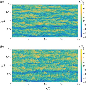
Figure 9 illustrates a sample of the instantaneous velocity and scalar fluctuation contours at
 $z/\unicode[STIX]{x1D6FF}=0.1$
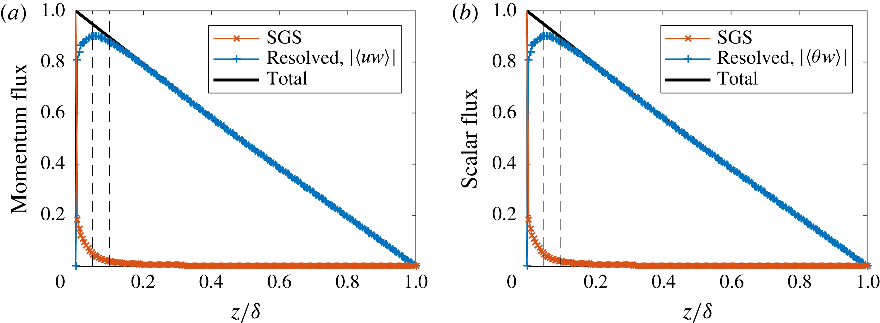
. As expected from the Reynolds analogy, the velocity field and the scalar concentration field are well correlated. Figure 10 shows the total and partial (resolved and SGS) values of the shear stress and wall-normal scalar flux, respectively. In the absence of viscous effects and under quasi-steady state conditions, the divergence of the total shear stress must balance the imposed pressure gradient. Also, the divergence of the total scalar flux must balance the rate of change in the scalar concentration. In this study, the half-channel flow is driven by a constant streamwise pressure gradient, and a constant scalar flux is imposed at the surface. Therefore, the total shear stress and wall-normal scalar flux are both expected to have linear mean profiles (Porté-Agel et al.
Reference Porté-Agel, Meneveau and Parlange2000; Porté-Agel Reference Porté-Agel2004). As shown in this figure, through the simulations, the linear profiles of the total turbulent fluxes are reproduced which can serve as a confirmation of statistical stationarity of the simulation results (Stoll & Porté-Agel Reference Stoll and Porté-Agel2006; Lu & Porté-Agel Reference Lu and Porté-Agel2013; Abkar et al.
Reference Abkar, Bae and Moin2016). As expected and seen in this figure, the contribution of the SGS parts in the total turbulent fluxes increase as the wall is approached. Beyond
 $z/\unicode[STIX]{x1D6FF}\approx 0.1$
, the LES grid resolves nearly all flux-carrying motions.
(a) Instantaneous velocity fluctuation contours at
 $z/\unicode[STIX]{x1D6FF}=0.1$
. (b) Same as (a) but for the scalar field.

Profiles of (a) the normalized (by
 $-u_{\unicode[STIX]{x1D70F}}^{2}$
) total and partial shear stress, and (b) the normalized (by
 $q_{z}|_{w}$
) total and partial wall-normal scalar flux. The two dashed vertical lines are at
 $z/\unicode[STIX]{x1D6FF}=0.05,0.1$
, respectively.

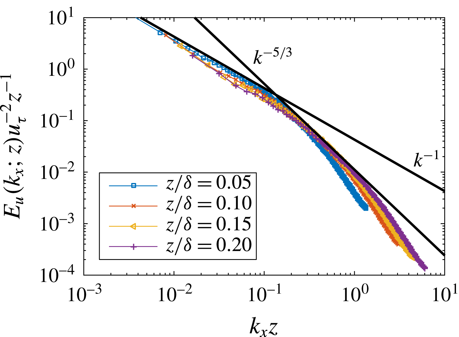
Figure 11 depicts the power spectra of the streamwise velocity at a few wall-normal locations and the flux-carrying component of the Reynolds stress. The
 $-1$
spectra (the energy spectrum of the streamwise velocity fluctuation decays as
 $k^{-1}$
) are captured and the LES grid resolves even part of the inertial range close to the wall.
Power spectra of the streamwise velocity at four wall-normal locations. The slopes of the two solid lines are
 $-1$
and
 $-5/3$
respectively.

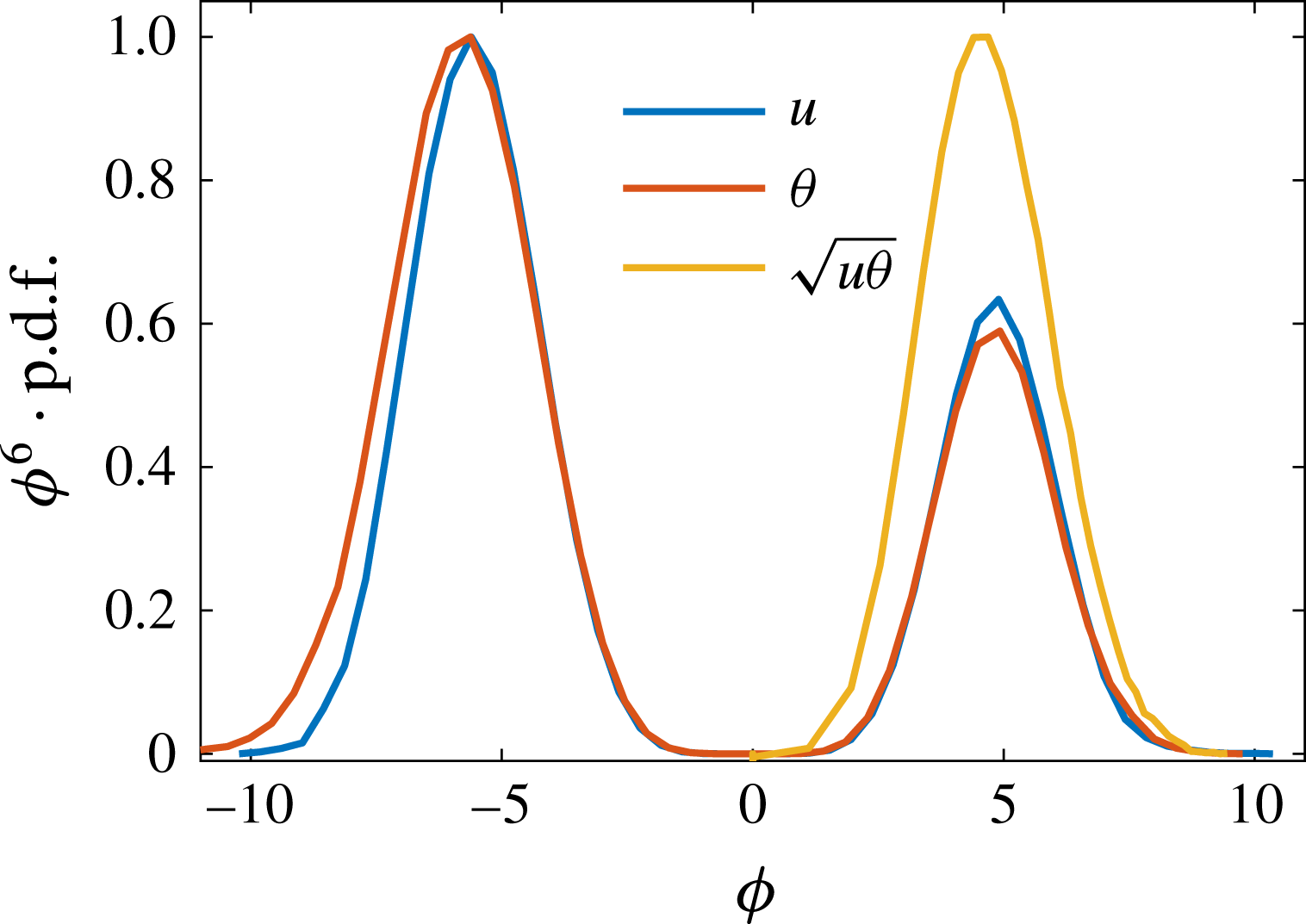
We will examine the usefulness of the HRAP hereafter. We will only consider statistics up to the sixth order since it is unlikely that statistics of higher order would be of any practical interest. In figure 12, data convergence is tested using the premultiplied probability density function (p.d.f.). Figure 12 shows the premultiplied p.d.f. of
 $u^{6}$
,
 $\unicode[STIX]{x1D703}^{6}$
and
 $(\sqrt{u\unicode[STIX]{x1D703}})^{6}$
. For both the velocity and scalar, it is more likely to encounter a large negative fluctuation than a large positive one (Stevens et al.
Reference Stevens, Wilczek and Meneveau2014).
 $\langle \unicode[STIX]{x1D719}^{6}\rangle$
is the area under the premultiplied p.d.f. of
 $\unicode[STIX]{x1D719}$
. Because the peaks in the premultiplied p.d.f.s are resolved for all the statistics,
 $\langle u^{6}\rangle$
,
 $\langle \unicode[STIX]{x1D703}^{6}\rangle$
,
 $\langle \unicode[STIX]{x1D703}^{3}u^{3}\rangle$
are statistically converged at this particular wall-normal distance. Premultiplied p.d.f.s at other wall-normal locations of other statistics are similar and are not shown here for brevity.
Premultiplied p.d.f.s of
 $\unicode[STIX]{x1D719}=u$
,
 $\unicode[STIX]{x1D703}$
,
 $\sqrt{\unicode[STIX]{x1D703}u}$
at
 $z/\unicode[STIX]{x1D6FF}=0.05$
. The premultiplied p.d.f.s are normalized by their respective peaks.

(a)
 $\langle u^{2}\rangle$
,
 $\langle \unicode[STIX]{x1D703}^{2}\rangle$
,
 $\langle u\unicode[STIX]{x1D703}\rangle$
as functions of the wall-normal distance. The dashed lines are at
 $z/\unicode[STIX]{x1D6FF}=0.05,0.3$
, respectively. The blue solid line indicates the slope
 $A_{1}=1.25$
, where
 $A_{1}$
is the Townsend–Perry constant. The orange and yellow lines indicate the logarithmic scalings of
 $\langle \unicode[STIX]{x1D703}^{2}\rangle$
and
 $\langle u\unicode[STIX]{x1D703}\rangle$
with slopes 1.5 and 1.2 respectively. The intercepts are 2.1, 0.95, 0.68 respectively for
 $\langle u^{2}\rangle$
,
 $\langle \unicode[STIX]{x1D703}^{2}\rangle$
and
 $\langle u\unicode[STIX]{x1D703}\rangle$
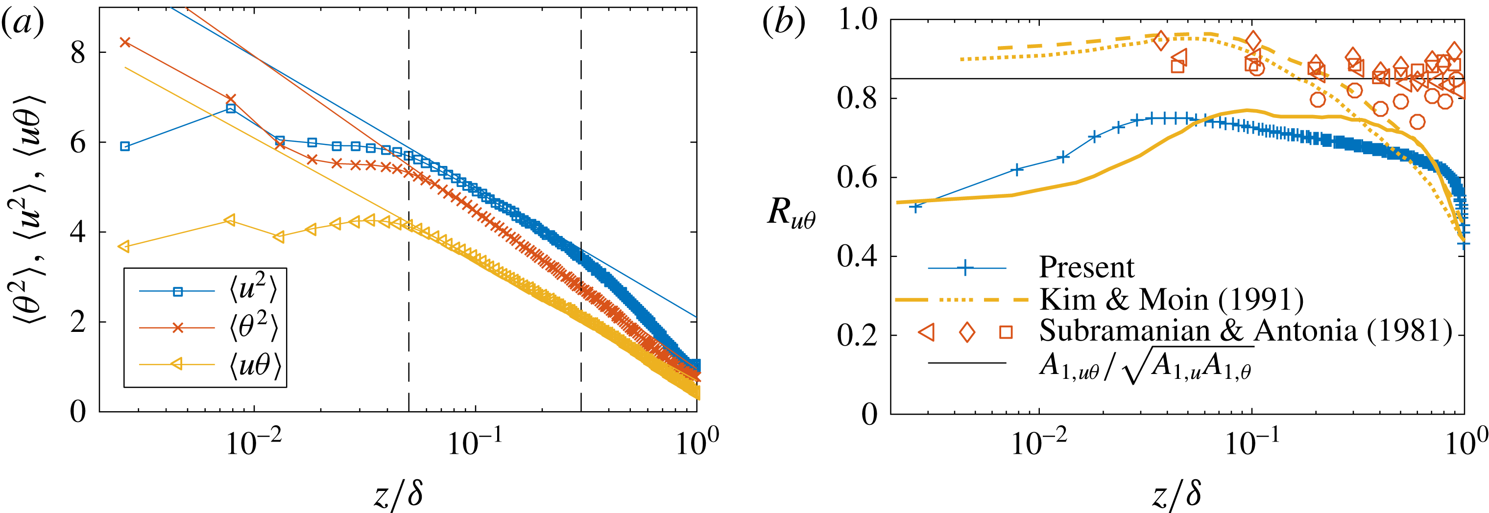
. (b) Correlation coefficient between the fluctuation of the passive scalar and the longitudinal velocity. Lines with ‘
 $+$
’ are from the present LES. ‘
 $+$
’:
 $R_{u\unicode[STIX]{x1D703}}=\langle u\unicode[STIX]{x1D703}\rangle /\sqrt{\langle u^{2}\rangle \langle \unicode[STIX]{x1D703}^{2}\rangle }$
. Lines are DNS by Kim & Moin (Reference Kim and Moin1989). ‘
 $-$
’:
 $Pr=0.1$
; ‘
 $--$
’:
 $Pr=0.71$
; ‘
 $\cdots \,$
’:
 $Pr=2$
. Symbols are experimental measurements by Subramanian & Antonia (Reference Subramanian and Antonia1981). ‘♢’:
 $Re_{\unicode[STIX]{x1D70F}}=290$
; ‘▫’:
 $Re_{\unicode[STIX]{x1D70F}}=560$
; ‘◃’:
 $Re_{\unicode[STIX]{x1D70F}}=1400$
; ‘◯’:
 $Re_{\unicode[STIX]{x1D70F}}=2300$
. The solid line corresponds to the asymptotic prediction according to the HRAP model,
 $A_{1,u\unicode[STIX]{x1D703}}/\sqrt{A_{1,\unicode[STIX]{x1D703}}A_{1,u}}\approx 0.85$
.

First, figure 13(a) shows the
 $\langle u^{2}\rangle$
,
 $\langle \unicode[STIX]{x1D703}^{2}\rangle$
and
 $\langle u\unicode[STIX]{x1D703}\rangle$
as functions of the wall-normal distance. Note the superscripts
 $+$
are dropped for brevity. The variance of the streamwise velocity follows the log law (with a slope
 $A_{1}\approx 1.25$
and a intercept
 $B_{1}\approx 2.1$
) in the region
 $0.05<z/\unicode[STIX]{x1D6FF}<0.3$
. The logarithmic regions of
 $\langle \unicode[STIX]{x1D703}^{2}\rangle$
and
 $\langle u\unicode[STIX]{x1D703}\rangle$
extend also from
 $z/\unicode[STIX]{x1D6FF}\approx 0.05$
to
 $z/\unicode[STIX]{x1D6FF}\approx 0.3$
. Because the velocity field subjects to a constant pressure gradient and the passive scalar is not forced, it is expected that the logarithmic region of
 $\langle \unicode[STIX]{x1D703}^{2}\rangle$
extends slightly further into the bulk region (Marusic et al.
Reference Marusic, Monty, Hultmark and Smits2013). The fact that the mixed second-order moment
 $\langle u\unicode[STIX]{x1D703}\rangle$
has a more extended logarithmic region than
 $\langle u^{2}\rangle$
suggests that the fluid motions that give rises to the logarithmic scalings are also responsible for the correlation between the passive scalar and the streamwise velocity fluctuations. In the present LES,
 $\langle \unicode[STIX]{x1D703}^{2}\rangle$
is slightly smaller than
 $\langle u^{2}\rangle$
, but the slope of
 $\langle \unicode[STIX]{x1D703}^{2}\rangle$
is slightly larger than that of
 $\langle u^{2}\rangle$
, suggesting
 $\langle \unicode[STIX]{x1D703}^{2}\rangle >\langle u^{2}\rangle$
asymptotically at high Reynolds numbers. The HRAP model does not provide a prediction for the exact value of those slopes but only the logarithmic scaling, therefore it is not clear whether
 $A_{1,u\unicode[STIX]{x1D703}}\approx A_{1,u}\approx A_{\unicode[STIX]{x1D703}}$
is just a coincidence (this is left for further investigation). Figure 13(b) shows the correlation coefficient between the scalar fluctuation and the velocity fluctuation as functions of the wall-normal distance from the present LES and the earlier measurements in the literature. Equation (2.6) suggests at high Reynolds numbers,
 $R_{u\unicode[STIX]{x1D703}}=\langle u\unicode[STIX]{x1D703}\rangle /\sqrt{\langle u^{2}\rangle \langle \unicode[STIX]{x1D703}^{2}\rangle }=A_{1,u\unicode[STIX]{x1D703}}/\sqrt{A_{1,\unicode[STIX]{x1D703}}A_{1,u}}\approx 0.85$
. This prediction agrees well with the experimental results reported in Subramanian & Antonia (Reference Subramanian and Antonia1981), where transport of a passive scalar in boundary-layer flows at friction Reynolds number
 $Re_{\unicode[STIX]{x1D70F}}$
from
 ${\approx}300$
to
 ${\approx}2100$
is considered. The DNS by Kim & Moin (Reference Kim and Moin1989) is at
 $Re_{\unicode[STIX]{x1D70F}}=180$
and the passive scalars are forced with a constant volumetric source term. Three molecular Prandtl numbers (i.e.
 $Pr=\unicode[STIX]{x1D708}/{\mathcal{D}}$
) are considered in Kim & Moin (Reference Kim and Moin1989), i.e.
 $Pr=0.1$
,
 $0.71$
,
 $2$
. We have included results of all three cases in figure 13 for comparison. The DNS provide data in the near-wall region, which are not available in experiments, but the results are affected by the finite Reynolds number effects. For
 $Pr=0.71$
,
 $2$
,
 $R_{u\unicode[STIX]{x1D703}}$
is approximately constant in the near-wall region and for
 $Pr=2$
,
 $R_{u\unicode[STIX]{x1D703}}$
is approximately constant in the bulk region. The asymptotic prediction
 $0.85$
is not a bad approximation even at
 $Re_{\unicode[STIX]{x1D70F}}=180$
. Last,
 $R_{u\unicode[STIX]{x1D703}}$
in the present LES is smaller (
 $R_{u\unicode[STIX]{x1D703}}\approx 0.65$
). This is probably because of a lack of large scales in the bulk region (this is clear in figure 13, where the slope of
 $\langle u^{2}\rangle$
is steeper in the bulk region than
 $\langle \unicode[STIX]{x1D703}^{2}\rangle$
). The effects of the Reynolds number, the flow configuration (boundary layer versus channel) and the forcing cannot be characterized using the available data and are left for further investigations.
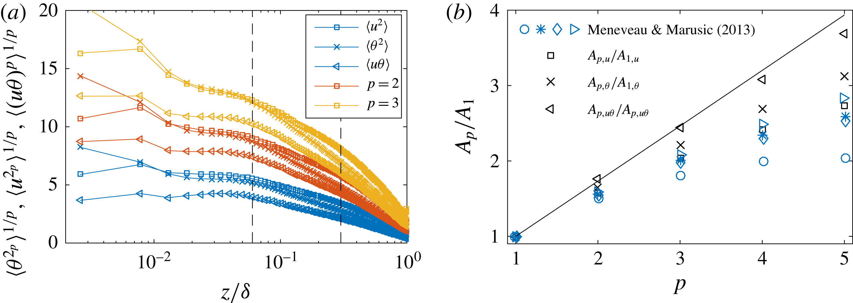
Figure 14(a) shows
 $\langle u^{2p}\rangle ^{1/p}$
,
 $\langle \unicode[STIX]{x1D703}^{2p}\rangle ^{1/p}$
and
 $\langle (u\unicode[STIX]{x1D703})^{p}\rangle ^{1/p}$
as functions of the wall-normal distance for
 $p=1,2,3$
. The logarithmic scalings are found in the region
 $z/\unicode[STIX]{x1D6FF}\gtrsim 0.05$
and
 $z/\unicode[STIX]{x1D6FF}\lesssim 0.3$
. The presence of a log region in these statistics supports the hierarchical random additive formalism for the passive scalar. Figure 14(b) shows the slopes of the log scalings as functions of the moment order. The HRAP model does not provide direct predictions for
 $A_{p}/A_{1}$
, however, by assuming the addends being Gaussian (following Kolmogorov (Reference Kolmogorov1962)),
 $A_{p}/A_{1}=[(2p-1)!!]^{1/p}$
, where
 $(\cdot )!!$
is the double factorial of the bracketed integer. This Gaussian prediction is included in figure 14(b) for comparison. The slopes of the even-order moments of the streamwise velocity fluctuation from the present LES (least square fit of the LES data in the region
 $0.06<z<0.3$
) are in good agreement with previous measurements (Meneveau & Marusic Reference Meneveau and Marusic2013). The slopes of the scalar even-order moments are not very different from the those of the velocity moments, and both
 $A_{p,\unicode[STIX]{x1D703}}/A_{1,\unicode[STIX]{x1D703}}$
and
 $A_{p,u}/A_{1,u}$
are sub-Gaussian. An exact analogy between
 $u$
and
 $\unicode[STIX]{x1D703}$
would imply
 $A_{u,p}=A_{\unicode[STIX]{x1D703},p}$
, which is certainly not inconsistent with the data. Although both the velocity and the scalar statistics are sub-Gaussian, the mixed quantity exhibits Gaussian behaviour. Since this sub-Gaussian behaviour is attributed to large-scale coherent motions within the boundary layer (Meneveau & Marusic Reference Meneveau and Marusic2013), figure 14(b) suggests those large-scale motions do not contribute to the velocity–scalar correlation.
(a) Even-order central moments (up to sixth order) of the longitudinal velocity, the passive scalar and the mixed single-point moments. Colours are used to differentiate between the order of the moments and symbols are used to differentiate between
 $u$
,
 $\unicode[STIX]{x1D703}$
and
 $\sqrt{u\unicode[STIX]{x1D703}}$
. The dashed lines are at
 $z/\unicode[STIX]{x1D6FF}=0.06,0.3$
respectively. (b) Slopes of the logarithmic scalings as functions of the moment order. The black symbols are from the present LES and the blue symbols are experimental measurements of the velocity log scalings (Meneveau & Marusic Reference Meneveau and Marusic2013). ‘◯’:
 $Re_{\unicode[STIX]{x1D70F}}=2900$
, ‘♢’:
 $Re_{\unicode[STIX]{x1D70F}}=3900$
, ‘
 $\ast$
’:
 $Re_{\unicode[STIX]{x1D70F}}=7300$
, ‘▹’:
 $Re_{\unicode[STIX]{x1D70F}}=19030$
. The solid line corresponds to the Gaussian prediction,
 $[(2p-1)!!]^{1/p}$
.

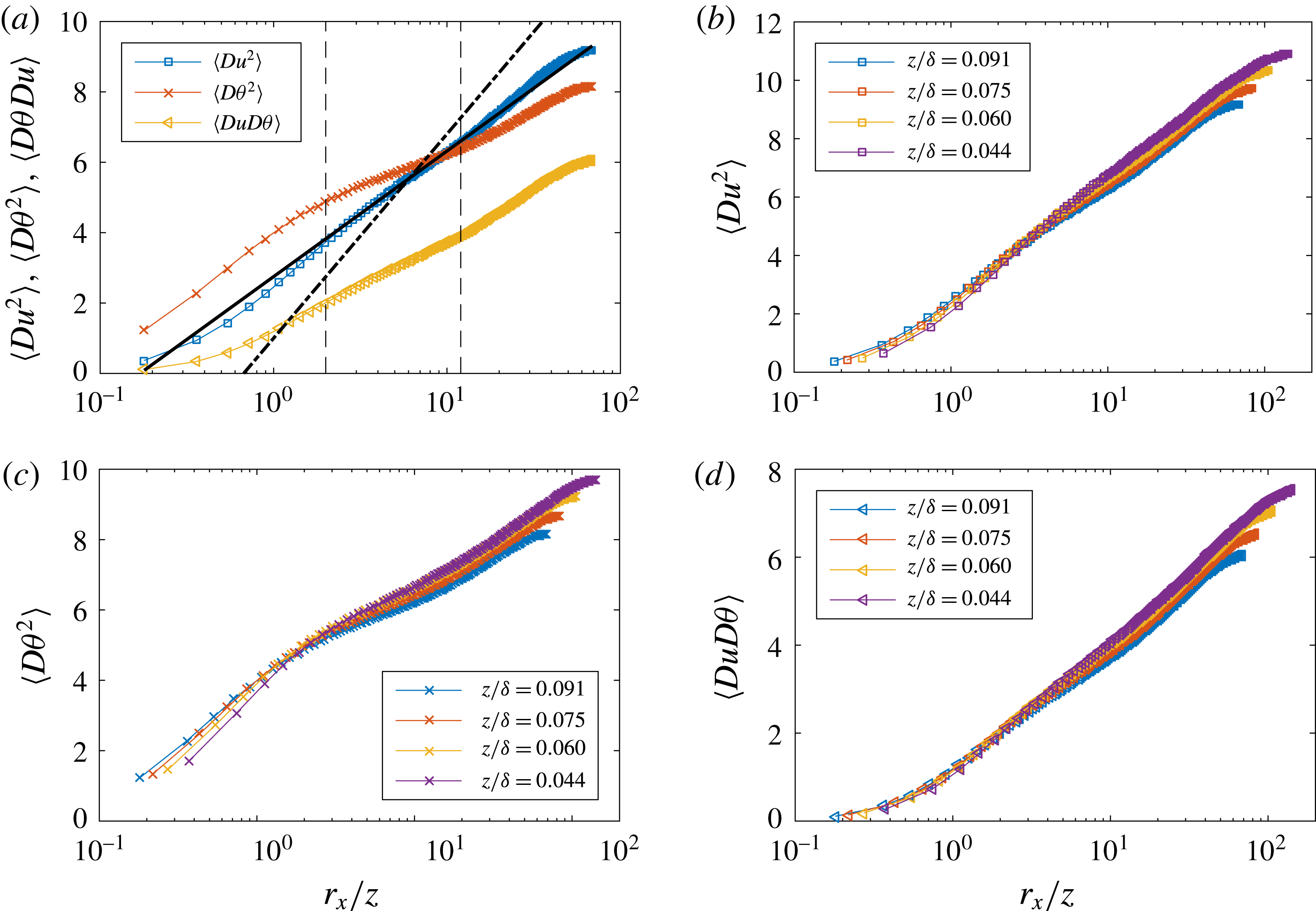
Next we examine statistics with a streamwise displacement. Figure 15(a) shows the second-order streamwise structure functions of the longitudinal velocity, the passive scalar and the mixed quantity of
 $\unicode[STIX]{x0394}u$
,
 $\unicode[STIX]{x0394}\unicode[STIX]{x1D703}$
as functions of the two-point displacements. Logarithmic scalings are found and the data support the HRAP model. Although the logarithmic scaling of the streamwise structure function was already reported in the work by de Silva et al. (Reference de Silva, Marusic, Woodcock and Meneveau2015), this is the first time this scaling is observed in an LES. The slope of the second-order structure function of the streamwise velocity is
 $2A_{1,u}\approx 2.5$
according to the HRAP model. This prediction is confirmed by high Reynolds number boundary-layer flow data (de Silva et al.
Reference de Silva, Marusic, Woodcock and Meneveau2015). In channel flows, however, the slope of
 $\langle Du^{2}\rangle$
is approximately
 $1.6$
(Yang et al.
Reference Yang, Baidya, Johnson, Maruisc and Meneveau2017a
), which in fact provides a good fit for the present LES data as well. The evidence is still not conclusive, but it is not impossible that the slope of
 $\langle Du^{2}\rangle$
in channel flow and in boundary-layer flow are different, even at high Reynolds numbers (see e.g. Hutchins & Marusic Reference Hutchins and Marusic2007a
). The slope of the logarithmic scaling of
 $\langle D\unicode[STIX]{x1D703}^{2}\rangle$
is smaller than that of
 $\langle Du^{2}\rangle$
, and the slope of the logarithmic scaling of the mixed structure function is in between. Figure 15(b,c,d) shows the second-order structure functions at four wall-normal locations,
 $z/\unicode[STIX]{x1D6FF}=0.044,0.060,0.075,0.91$
. According to the HRAP (and as is clear in figure 2), structure functions collapse as functions of
 $r_{x}/z$
in the log region. The data collapse reasonably well for all the statistics.
(a) Second-order streamwise structure functions
 $\langle Du^{2}\rangle =\langle (u(x)-u(x+r))^{2}\rangle$
,
 $\langle D\unicode[STIX]{x1D703}^{2}\rangle =\langle (\unicode[STIX]{x1D703}(x)-\unicode[STIX]{x1D703}(x+r))^{2}\rangle$
,
 $\langle DuD\unicode[STIX]{x1D703}\rangle =\langle (u(x)-u(x+r))(\unicode[STIX]{x1D703}(x)-\unicode[STIX]{x1D703}(x+r))\rangle$
at
 $z/\unicode[STIX]{x1D6FF}=0.091$
. The two vertical lines are at
 $r_{x}/z=2,12$
. The dot-dashed line indicates the slope
 $2A_{1}\approx 2.5$
and the solid line indicates the slope 1.6. (b) Second-order streamwise velocity structure function at various wall-normal locations (colour available on line). (c) Same as (b) but for the passive scalar. (d) Same as (b) but for the mixed structure function.

High-order structure functions are examined at
 $z/\unicode[STIX]{x1D6FF}=0.044$
, which corresponds to the ninth grid point away from the wall and there LES solutions are not affected by the wall boundary condition nor by the large-scale fluid motions. This near-wall location also allows an extended logarithmic region from
 $r\sim z$
to
 $r\sim \unicode[STIX]{x1D6FF}$
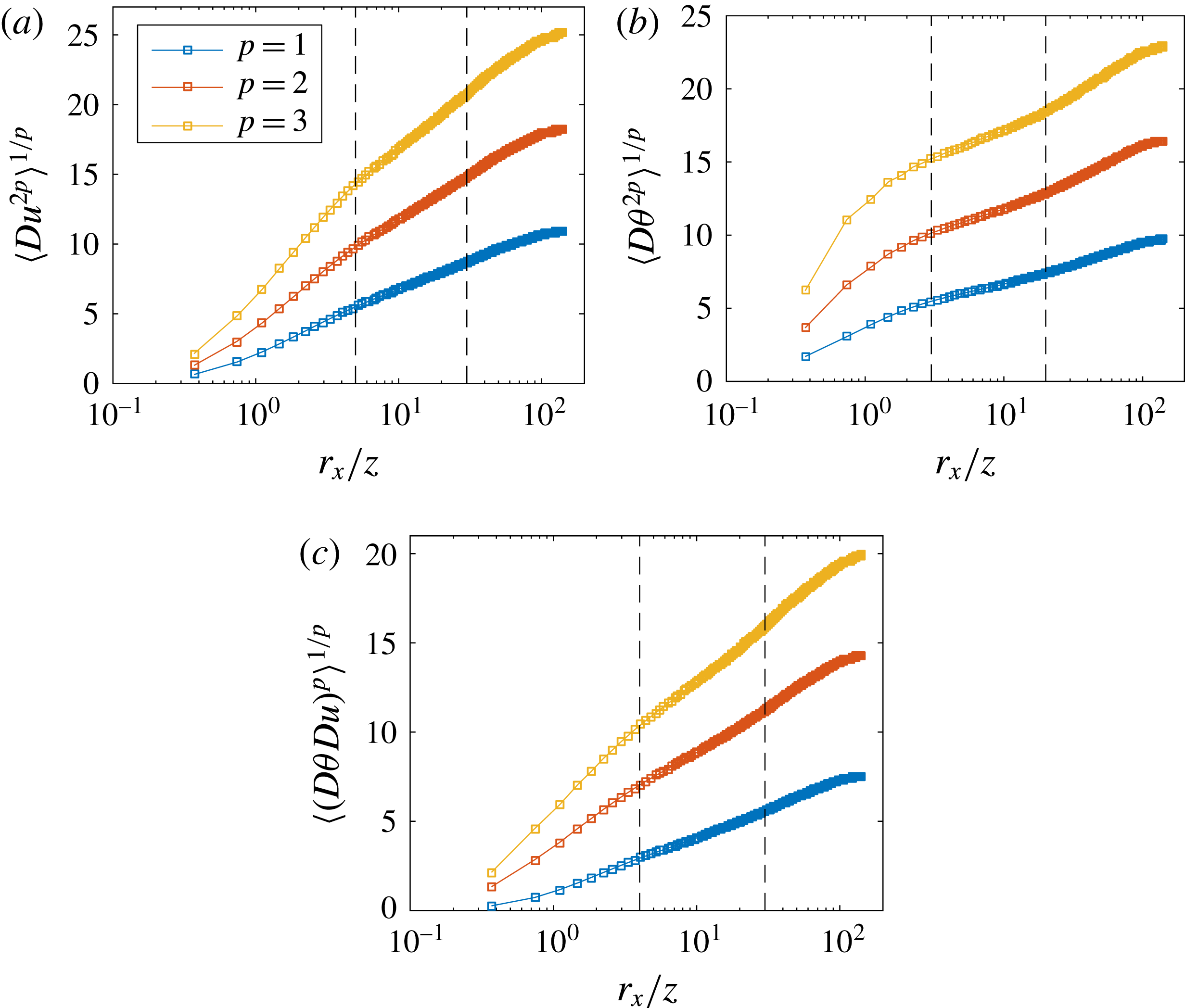
. Figure 16(a–c) shows
 $\langle Du^{2p}\rangle ^{1/p}$
,
 $\langle D\unicode[STIX]{x1D703}^{2p}\rangle ^{1/p}$
,
 $\langle Du^{p}D\unicode[STIX]{x1D703}^{p}\rangle ^{1/p}$
as functions of
 $r_{x}/z$
for
 $p=1,2,3$
. The logarithmic regions of the high-order statistics are narrower than their second-order counterparts, however, log scalings can still be seen in
 $5<r_{x}/z<30$
. The slopes of the velocity and mixed structure functions increases as a function of
 $p$
. Because structure functions account for only attached eddies whose sizes are such that they affect only one of the two points, the presence of the logarithmic scalings in figures 15 and 16 support the hierarchical description for these eddies. Whether the HRAP model can be used to model the attached eddies whose sizes are such that they could affect both points simultaneously must be tested using the
 $\log (\unicode[STIX]{x1D6FF}/r)$
scalings.
(a)
 $\langle Du^{2p}\rangle ^{1/p}$
for
 $p=1,2,3$
at
 $z/\unicode[STIX]{x1D6FF}=0.091$
. (b) Same as (a) but for
 $D\unicode[STIX]{x1D703}$
. (c) Same as (a) but for the mixed structure function.

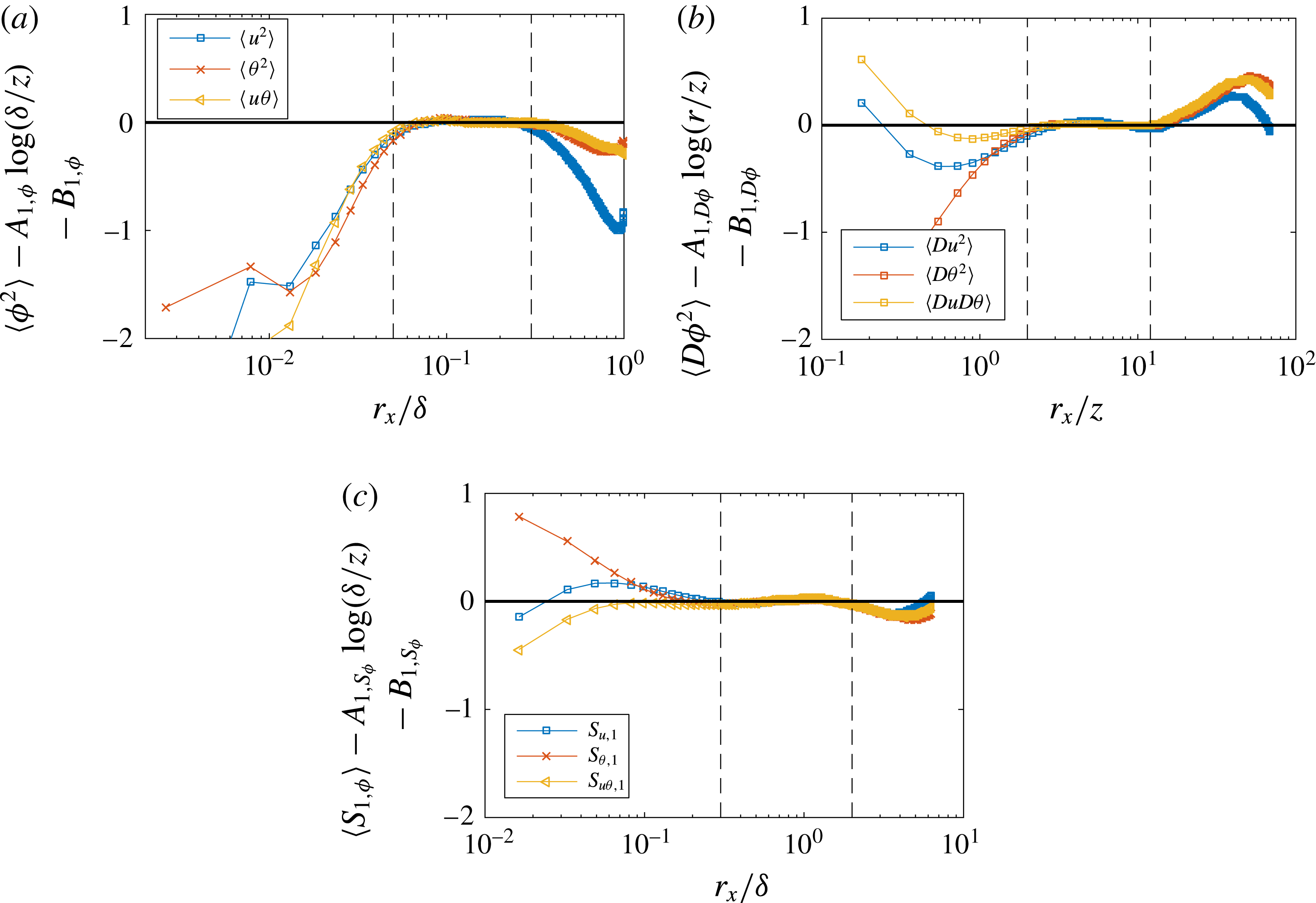
The analogy between the streamwise velocity fluctuation and the fluctuation in passive scalars is so far supported by the data, and the HRAP model has also provided reasonably realistic estimates of the statistics. Next we will examine the scalings in (2.13)–(2.15), its scalar counterpart and (2.10)–(2.12). These logarithmic scalings are denoted as
 $S_{\unicode[STIX]{x1D719},p}$
for brevity with
 $\unicode[STIX]{x1D719}=u,\unicode[STIX]{x1D703},u\unicode[STIX]{x1D703}$
indicating the velocity, the passive scalar and the mixed statistics;
 $p$
indicates the statistics order. Note
 $S_{\unicode[STIX]{x1D719},1}$
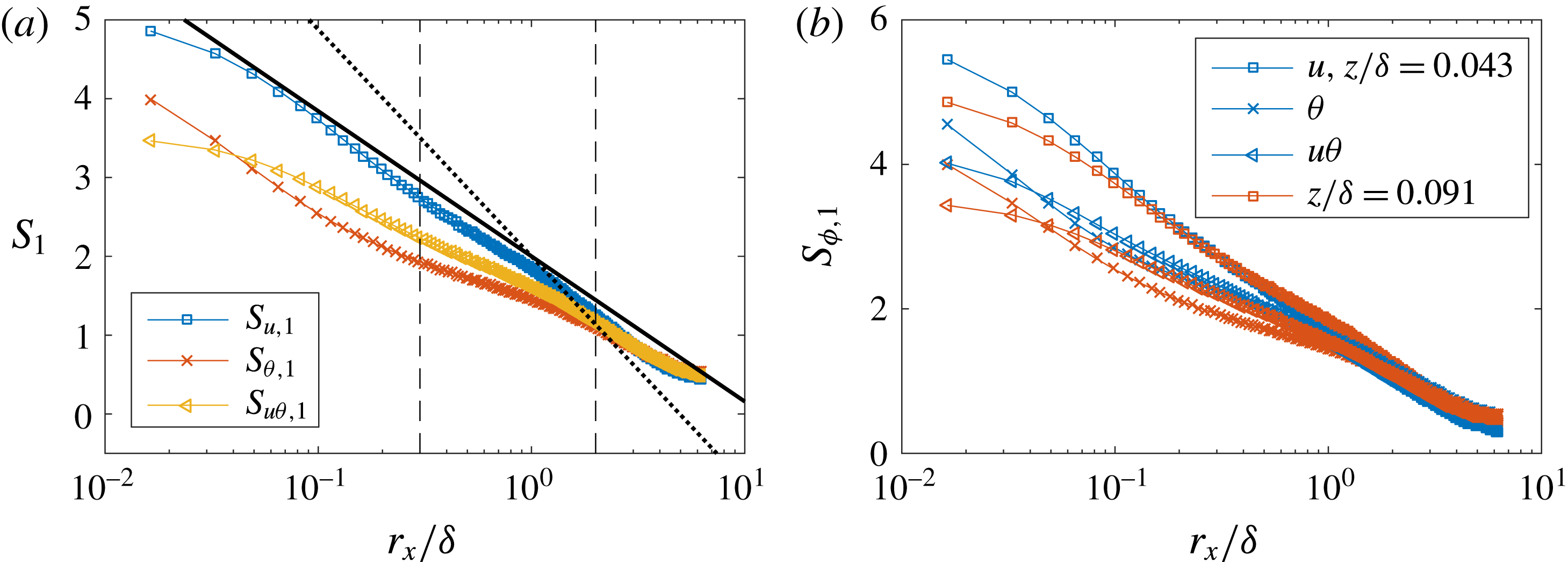
is the two-point correlation in the streamwise direction. Figure 17(a) shows
 $S_{u,1}$
,
 $S_{\unicode[STIX]{x1D703},1}$
,
 $S_{u\unicode[STIX]{x1D703},1}$
as functions of the two-point displacements. Logarithmic scalings are found between
 $0.3<z/\unicode[STIX]{x1D6FF}<2$
(the log region of the mixed two-point correlation and the velocity correlation appear to extend to smaller displacements). The slope of the logarithmic scaling of
 $\langle u(x)u(x+r)\rangle$
is 0.8 in channel flow (Yang et al.
Reference Yang, Baidya, Johnson, Maruisc and Meneveau2017a
). The LES results agrees with the DNS, showing a similar slope in the enclosed region. The expected slope for the two-point velocity correlation is
 $A_{1}=1.25$
and is half of the slope of
 $\langle Du^{2}\rangle$
. The measured slope of
 $S_{u,1}$
is
 ${\approx}0.8$
, which is smaller than the prediction according to the HRAP, but is in fact approximately half of the slope of
 $\langle Du^{2}\rangle$
. The slopes of
 $S_{\unicode[STIX]{x1D703},1}$
and
 $S_{u\unicode[STIX]{x1D703},1}$
are 0.4 and 0.5, respectively, which are also half of the slopes of
 $\langle D\unicode[STIX]{x1D703}^{2}\rangle$
,
 $\langle DuD\unicode[STIX]{x1D703}\rangle$
. According to the HRAP model,
 $S_{\unicode[STIX]{x1D719},1}$
collapse as functions of
 $r_{x}/\unicode[STIX]{x1D6FF}$
. This is examined in figure 17(b), where
 $S_{\unicode[STIX]{x1D719},1}$
at
 $z/\unicode[STIX]{x1D6FF}=0.043,0.091$
are plotted as functions of
 $r_{x}/\unicode[STIX]{x1D6FF}$
. Reasonable data collapse is found for
 $S_{\unicode[STIX]{x1D719},1}$
at the two wall-normal locations at large
 $r_{x}$
. Because
 $\log (\unicode[STIX]{x1D6FF}/r)$
scalings account only for attached eddies whose sizes are sufficiently large that they could affect both points simultaneously, the presence log scalings in figure 17 suggests that those large attached eddies follow also the hierarchical description provided in the HRAP formalism.
(a)
 $S_{u,1}$
,
 $S_{\unicode[STIX]{x1D703},1}$
,
 $S_{u\unicode[STIX]{x1D703},1}$
at
 $z/\unicode[STIX]{x1D6FF}=0.091$
. The solid line indicates the slope
 $A_{1}=0.8$
. The two dashed lines are at
 $z/\unicode[STIX]{x1D6FF}=0.3$
and
 $z/\unicode[STIX]{x1D6FF}=2$
. The dotted line indicates the slope
 $A_{1}=1.25$
. (b)
 $S_{u,1}$
,
 $S_{\unicode[STIX]{x1D703},1}$
,
 $S_{u\unicode[STIX]{x1D703},1}$
at
 $z/\unicode[STIX]{x1D6FF}=0.091$
at two wall-normal heights. Colours are used to differentiate between different wall-normal heights and symbols are used to differentiate between different statistics.

Before we conclude, the quality of the logarithmic scalings is examined by compensating the statistics with the expected logarithmic scaling. In figure 18, we show the compensated logarithmic scalings. Only low-order statistics are shown here for brevity and similar results are found for high-order statistics. A (reasonably) flat region can be found within the enclosed region for each logarithmic scaling examined above.
Compensated logarithmic scalings. (a) Compensated scalings of the single-point second-order moments.
 $\unicode[STIX]{x1D719}$
is
 $u$
,
 $\unicode[STIX]{x1D703}$
or
 $u\unicode[STIX]{x1D703}$
. (b) Compensated scalings of the second-order structure functions.
 $A_{1,D\unicode[STIX]{x1D719}}$
,
 $B_{1,D\unicode[STIX]{x1D719}}$
are constants of the respective logarithmic scalings and are fitted within the enclosed region. (c) Compensated scaling of the two-point correlations.
 $A_{1,S_{\unicode[STIX]{x1D719}}}$
,
 $B_{1,S_{\unicode[STIX]{x1D719}}}$
are constants as well. The black lines are at
 $0$
. The extend of the
 $y$
-axis are the same for all the plots for a fair comparison.

Last we examine the correlations as defined in (2.17) in figure 19. As no measurements could be found in the literature, only results from the present LES are shown. The HRAP formalism predicts an
 $r_{x}$
-independent correlation for both
 $R_{2}=\langle DuD\unicode[STIX]{x1D703}\rangle /\sqrt{\langle Du^{2}\rangle \langle D\unicode[STIX]{x1D703}^{2}\rangle }$
and
 $R_{3}=0.5\langle u(x)\unicode[STIX]{x1D703}(x+r)+u(x+r)\unicode[STIX]{x1D703}(x)\rangle /\sqrt{\langle u(x)u(x+r)\rangle \langle \unicode[STIX]{x1D703}(x)\unicode[STIX]{x1D703}(x+r)\rangle }$
. The measured
 $R_{2}$
falls below this prediction and the measured
 $R_{3}$
is above.
 $R_{3}$
is approximately constant, but
 $R_{2}$
increases from
 $R_{2}=0.2$
at small
 $r_{x}$
to
 $R_{2}=0.7$
at large
 $r_{x}$
.
 $R_{2}$
,
 $R_{3}$
evaluated at
 $z/\unicode[STIX]{x1D6FF}=0.091$
as functions of the two-point displacements. The HRAP predicts
 $R_{2}=R_{3}=A_{1,u\unicode[STIX]{x1D703}}/\sqrt{A_{1,u}A_{1,\unicode[STIX]{x1D703}}}\approx 0.85$
and this prediction is indicated using a thin solid line.

In this section, we have confirmed the three sets of logarithmic scalings
 $\log (\unicode[STIX]{x1D6FF}/z)$
,
 $\log (r_{x}/z)$
and
 $\log (\unicode[STIX]{x1D6FF}/r_{x})$
, which are admitted by the HRAP model for both the passive scalar and the mixed quantity of the scalar and the streamwise velocity. The analogy between the longitudinal velocity and the passive scalar is supported and the scalar kinematics is well modelled by the hierarchical model HRAP (and certainly also the attached-eddy hypothesis).
6 Concluding remarks
In this work, we show that the fluctuations of a fully developed passive scalar in wall-bounded flows at high Reynolds number can be modelled using the HRAP formalism, which was previously used for the modelling of velocity fluctuations in high Reynolds number wall turbulence. We examined and confirmed a few logarithmic scalings for the passive scalar and the mixed quantity, which scalings were established only for the velocity before. The correlation coefficient
 $R_{u\unicode[STIX]{x1D703}}$
is
 ${\approx}0.85$
in the log region at high Reynolds numbers according to the HRAP. This is supported, at least qualitatively by the currently available data. The LES results generally support the analogy between the streamwise velocity fluctuation and the fluctuation of the passive scalar. The present LES suggests
 $A_{1,u}\approx A_{1,\unicode[STIX]{x1D703}}\approx A_{1,u\unicode[STIX]{x1D703}}$
(see figure 13). The HRAP model may be leveraged to model the near-wall turbulence in a wall-modelled LES, where eddies of constant heights in inner units become successively subgrid as the Reynolds number increases. Besides, the analogy suggests that the attached eddies that dominate the velocity kinematics in the log region control also the kinematics of the passive scalar, providing a framework for modelling scalar transport in wall-bounded flows.
The streamwise logarithmic scalings including
 $\langle Du^{2}\rangle \sim \log (r_{x}/z)$
and
 $\langle u(x)u(x+r_{x})\rangle \sim \log (\unicode[STIX]{x1D6FF}/r_{x})$
are firstly captured in an LES calculation. The LES also suggests a slope
 ${\approx}1.6$
for the log scaling
 $\langle Du^{2}\rangle$
which is consistent with previous measurements using DNS of channel flow, but is smaller than the observed slope in boundary-layer flows.
Last, it is worth noting that the scalar turbulence in wall-bounded turbulence is a research topic of its own merits (also see e.g. Watanabe & Gotoh Reference Watanabe and Gotoh2004; Lavertu & Mydlarski Reference Lavertu and Mydlarski2005; Talluru et al. Reference Talluru, Hernandez-Silva, Philip and Chauhan2017), although the efforts here have tried to model the scalar using knowledge we have gained on the velocity turbulence.
Acknowledgements
X.Y. was funded by the US AFOSR (grant no. 1194592-1-TAAHO). M.A. was supported by the NASA (grant no. NNX15AU93A). The authors are grateful to Professor P. Moin for his insightful comments on the manuscript.