Introduction
In the past two decades, tremendous progress has been made on developing theories for the kinematics of dislocation densities.[Reference Acharya1–Reference Hochrainer, Zaiser and Gumbsch4] Of special importance is the equation  ${\dot {\bi \alpha}} = - \vec \nabla \times ({\bi \alpha} \times \vec v)$ for the evolution of the Nye tensor[Reference Nye5] α proposed initially by Kröner[Reference Kröner6] and further developed by Acharya,[Reference Acharya1] and a “continuous dislocation dynamics” (CDD) theory proposed by Hochrainer et al.,[Reference Hochrainer, Zaiser and Gumbsch4] in which the key concept is the involvement of dislocation curvature as a second field variable in addition to dislocation density itself. However, there has been no documented attempt to reconcile these two important theories. Recently, the present author has also proposed an evolution scheme for dislocation densities based on consideration of the approach and tilting of single dislocations forming the dislocation densities.[Reference Leung and Ngan7] In this paper, we show that Leung and Ngan's scheme[Reference Leung and Ngan7] is fully consistent with Acharya's equation[Reference Acharya1] and the CDD theory.[Reference Hochrainer, Zaiser and Gumbsch4] Moreover, we show that the curvature variable in CDD is unnecessary if divergence of dislocation flux is counted one-dimensionally along the dislocation velocity direction, rather than two-dimensionally over the slip plane as in the CDD. Furthermore, we also present a clear delineation of how discrete dislocations would form coarse-grained densities, and how the evolution of densities can be derived from the movement of the comprising individual dislocations—this is an aspect which is not clear in Acharya's equation, which deals only with geometrically necessary dislocations.
Before we begin, a note on nomenclature will be useful. First, by a “discrete” dislocation representation, we mean a single dislocation without any description of the evolution of the dislocation core itself. A “discrete” dislocation therefore has its contents represented by a δ-like function that does not change shape with space or time as the entire dislocation moves, and is therefore different from an “intensive” dislocation representation in which the Burgers vector distribution in the dislocation core is described in detail as in the Peierls–Nabarro model. In this paper, we will first derive the evolution of discrete dislocations in terms of their density fields, before we consider the evolution of coarse-grained dislocation densities.
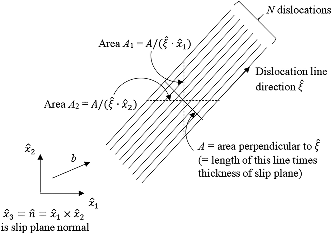
Area density of dislocations on a slip plane.

Secondly, by “dislocation density”, we refer to the number of dislocations threading unit area, which is a vector quantity with unit m−2 since the unit area is specified by its normal direction. This “area” definition is that used in the Nye tensor,[Reference Acharya1] which is the Burgers vector content threading unit area. Consider a group of dislocations that are momentarily straight and parallel to each other within a small pixel of the slip plane (Fig. 1). For an area A perpendicular to the dislocation lines, the area density of dislocations is therefore:
 $$\rho = N/A.$$
Since A is perpendicular to the dislocations, the ρ defined this way is not only the area density, but also the volume density of dislocation length per unit volume (a scalar). This can be seen by considering the dislocation length inside a control volume of A × dξ, where dξ is a small length along the dislocation direction  $\hat \xi $. For areas A 1 and A 2 perpendicular to two orthonormal axes
 $\hat x_1 $ and
 $\hat x_2 $ generally placed on the slip plane, respectively, the same N dislocations correspond to area densities:
 $$\rho _1 = \displaystyle{N \over {A/(\hat \xi \cdot \hat x_1 )}} = \rho (\hat \xi \cdot \hat x_1 ) = \vec \rho \cdot \hat x_1 ;\quad \rho _2 = \vec \rho \cdot \hat x_2,$$
where the vector  $\vec \rho $ is defined as
 $\vec \rho = \rho \; \hat \xi $. Since the factors
 $\hat \xi \cdot \hat x_1 $ and
 $\hat \xi \cdot \hat x_2 $ are ≤1, ρ 1 and ρ 2 are ≤ ρ, and since
 $\hat x_1 $ and
 $\hat x_2 $ are arbitrary orthonormal directions on the slip plane, ρ as defined in Eq. (1) (with A being the area normal to the dislocations) is the maximum possible area density. Equation (2a) also implies that
 $$\vec \rho = \rho _1 \hat x_1 + \rho _2 \hat x_2 ;\quad \rho = \left \vert {\vec \rho} \right \vert = \sqrt {\rho _1^2 + \rho _2^2}.$$
Equation (2a), which can be further written in the form
 $$\rho _j = \rho (\hat \xi \cdot \hat x_j ),$$
gives the relation between a general area density ρ j (number of dislocations threading unit area normal to  $\hat x_j $) and the volume density ρ. When
 $\hat x_j $ is along
 $\hat \xi $, ρ j = ρ, which is also the maximum area density.
In the following, we will first discuss Acharya's equation and modify it into a form more useful for our next development. Then, we will discuss the density vector field of discrete dislocations as proposed by Leung and Ngan,[Reference Leung and Ngan7] and prove that it satisfies Acharya's equation.[Reference Acharya1] We will then derive the coarse-grained densities of dislocations and their evolution equation based on combined contributions from discrete dislocations. Then, finally, we will show that the evolution equation for coarse-grained densities is consistent with CDD.[Reference Hochrainer, Zaiser and Gumbsch4]
Evolution equation for Nye tensor
The kinematics of line objects moving in and out of threaded areas over which line densities are counted is encountered in classical physics such as electromagnetic induction. The well-known Maxwell–Faraday equation can be cast in the following form  $\partial \vec B/\partial t = - \vec \nabla \times (\vec B \times \vec v)$ for the magnetic flux lines
 $\vec B$ moving with velocity
 $\vec v$. This equation applies equally well to dislocations;[Reference Acharya1, Reference Kröner6] thus, in terms of the dislocation density and Nye tensor,[Reference Nye5] their evolution equations are, respectively:
 $$\dot {\vec \rho} = - \vec \nabla \times (\vec \rho \times \vec v)$$
and
 $${\dot {\bi \alpha}} = - \vec \nabla \times ({\bi \alpha} \times \vec v),$$
where the Nye tensor is such that
 $$\alpha _{ij} = b_i \rho _j, \;{\rm or}\;{\bi \alpha} = {\bi \;} \vec b{\bi \;} \otimes {\bi \;} \vec \rho, $$
which gives the Burgers vector b i along i threading unit plane with normal j. In Eq. (4), it is understood that the cross product in  ${\bi \alpha} \times \vec v$ is between each row i of α and
 $\vec v$, i.e.,
 $({\bi \alpha} \times \vec v)_{il} = \alpha _{ij} v_k \epsilon _{ijl} \hat x_l $, or
 ${\bi \alpha} \times \vec v = (\vec b \otimes \vec \rho ) \times \vec v = \vec b \otimes (\vec \rho \times \vec v)$, and the curl “
 $\vec \nabla \times $” also operates on each row of the tensor
 ${\bi \alpha} \times \vec v$—such operations on each row i of α deal with the conservation of each component b i of the Burgers vector contents carried by the dislocation lines as they move in space. With these, Eq. (4) is mathematically compatible with Eq. (3): in Eq. (4),
 ${\dot {\bi \alpha}} = \vec b \otimes \dot {\vec \rho} {\bi \;} $ and
 ${\bi \alpha} \times \vec v = (\vec b{\bi \;} \otimes {\bi \;} \vec \rho ) \times \vec v = \vec b{\bi \;} \otimes {\bi \;} (\vec \rho \times \vec v)$, and hence, Eq. (4) becomes
 $${\dot {\bi \alpha}} = \vec b \otimes \dot {\vec \rho} = - \vec \nabla \times [\vec b \otimes (\vec \rho \times \vec v)] = - \vec b \otimes [\vec \nabla \times (\vec \rho \times \vec v)],$$
which then reduces to Eq. (3) by crossing out the constant  $\vec b$ from both sides of the equation.
For dislocations gliding on a slip plane with normal  $\hat n$, the dislocation velocity
 $\vec v$ has to be perpendicular to the dislocation line
 $\hat \xi $ and lying on the slip plane, i.e.,
 $$\vec v = v\; (\hat n \times \hat \xi ),$$
where v is the magnitude of  $\vec v$. Therefore,
 $\vec \rho \times \vec v = \rho v\; \hat n$, and so Eq. (3) reduces to
 $$\dot {\vec \rho} = - \vec \nabla \times (\rho v \hat n).$$
Equation (7) is the evolution equation for the dislocation density on a single slip plane, based on the general conservation law in Eq. (3), as well as the condition of orthogonal movement of dislocations in Eq. (6). With the Cartesian coordinates shown in Fig. 1,  $\hat x_3 = \hat x_1 \times \hat x_2 \; $ is the slip plane normal
 $\hat n$, and hence Eq. (7) gives
 $$\dot {\vec \rho} = \dot \rho _1 \hat x_1 + \dot \rho _2 \hat x_2 = - \displaystyle{{\partial (\rho v)} \over {\partial x_2}} \hat x_1 + \displaystyle{{\partial (\rho v)} \over {\partial x_1}} \hat x_2, $$
or,
 $$\dot \rho _1 = - \displaystyle{{\partial (\rho v)} \over {\partial x_2}} ;\quad \dot \rho _2 = \displaystyle{{\partial (\rho v)} \over {\partial x_1}} ;\quad \rho = \sqrt {\rho _1^2 + \rho _2^2}. $$
Equation (8) automatically guarantees dislocation connectivity governed by  $\vec \nabla \cdot \vec \rho = 0$. To see this, Eq. (8) readily gives
 $$\vec \nabla \cdot \dot {\vec \rho} = - \displaystyle{{\partial ^2 (\rho v)} \over {\partial x_1 \partial x_2}} + \displaystyle{{\partial ^2 (\rho v)} \over {\partial x_1 \partial x_2}} = 0. $$
Hence, given that  $\vec \nabla \cdot \vec \rho = 0$ at time t = 0, then
 $\vec \nabla \cdot \vec \rho = 0$
 $\forall t$. Furthermore, Eq. (8) indicates that the flux ρv serves as the stream function for the density flow
 $\dot {\vec \rho} $. From Eq. (8),
 $\dot {\vec \rho} \cdot \vec \nabla (\rho v) = (\dot \rho _1 \hat x_1 + \dot \rho _2 \hat x_2 ) \cdot (\dot \rho _2 \hat x_1 - \dot \rho _1 \hat x_2 ) = 0$, which means that
 $\dot {\vec \rho} $ is perpendicular to
 $\vec \nabla (\rho v)$, or
 $\dot {\vec \rho} $ points along constant (ρv) curves.
While Eq. (4) provides a very general evolution law for the Nye tensor α, to clearly delineate the effects of geometrically necessary dislocations (GNDs) versus those of the statistically stored dislocations (SSDs), Acharya and Roy[Reference Acharya and Roy8] coarse-grained Eq. (4) into:
 $${\dot {\bi \alpha}} = - \vec \nabla \times ({\bi \alpha} \times \vec v) = - \vec \nabla \times ({\bi \alpha} \times \vec v + {\bi L}^{\bi p} ),$$
where  ${\rm \langle} \cdots {\rm \rangle} = {\rm \langle} \cdots {\rm \rangle} (\vec r,t)$ denotes a coarse-grained average of quantity ( · · · ), namely, an average of ( · · · ) over a small space and time domain about the field point
 $\vec r$ and time t, and Lp is defined as
 ${\bi \alpha} \times \vec v - {\bi \alpha} \times \vec v$. Therefore, α represents the GND contents of the dislocation population, and Lp represents the flux of the SSDs. However, the evolution of Lp is not exactly known, and so far, only phenomenologic laws were used to describe it.[Reference Acharya and Roy8, Reference Taupin, Varadhan, Fressengeas and Beaudoin9]
Density field for discrete dislocation on slip plane
While Acharya's Eq. (10) serves to by-pass detailed consideration of the kinematics of the individual dislocations comprising a dislocation density, it is thought here that defining clearly the relationship between the properties of the coarse-grained dislocation density and those of the comprising discrete dislocations is indeed very important for a density-based theory. It is therefore the purpose of this section to first derive the evolution of the density field of discrete dislocations, so that, in the next section, the evolution of dislocation densities can be derived.
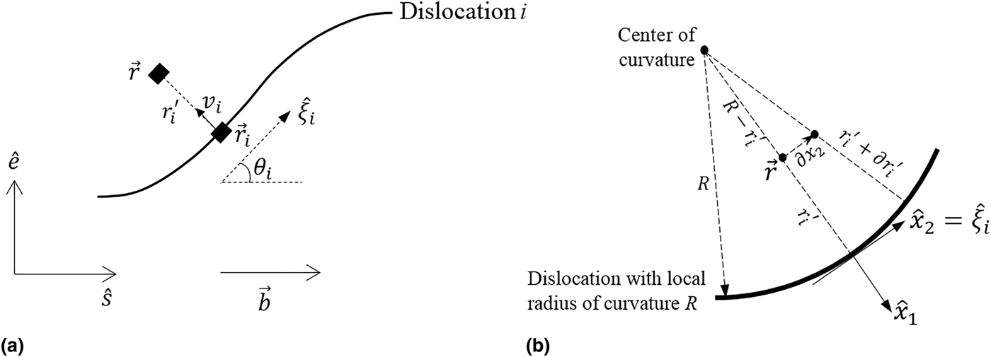
Consider a general curved dislocation i lying on the slip plane as shown in Figs. 2(a) and 2(b). Leung and Ngan[Reference Leung and Ngan7] recently proposed the following vector field of the dislocation density:
 $$\vec \rho _i (\vec r) = \delta (r_i {\rm ^{\prime}})\hat \xi _i /b = \delta (r_i {\rm ^{\prime}})(\sin \theta _i \hat e + \cos \theta _i \hat s)/b,$$
where  $\vec r = (x,y)$ is a general field point on the slip plane,
 $r_i {\rm ^{\prime}}$ is the shortest (perpendicular) distance from
 $\vec r$ to the dislocation curve,
 $\hat \xi _i = (\sin \theta _i \hat e + \cos \theta _i \hat s)$ is the local tangent direction of the dislocation at the point closest to
 $\vec r$ with θ i being the dislocation character there, b is the atomic thickness of the slip plane, and
 $\delta (r_i {\rm ^{\prime}})$ is a δ-like function that describes the core distribution of the dislocation. Essentially, Eq. (11) says that the vector field
 $\vec \rho _i (\vec r)$ is zero everywhere except when on the dislocation line (
 $r_i {\rm ^{\prime}} = 0$) where
 $\vec \rho _i = \hat \xi _i /b$. (The b here is to ensure that
 $\left\vert {\vec \rho _i} \right\vert$ has the meaning of one dislocation per cross-section of the slip plane.)
Here, we show that Eq. (11) satisfies Eq. (7) or (8). By re-writing Eq. (11) as
 $$\vec \rho _i (\vec r) = \rho _i (r_i {\rm ^{\prime}})\hat \xi _i, $$
where  $\rho _i (r_i {\rm ^{\prime}}) = \delta (r')/b$, its time derivative is
 $$\eqalign{& \dot {\vec \rho} _{\bi i} = - \rho _i^{\prime} (r_i {\rm ^{\prime}})v_i \; \hat \xi _i + \rho _i (r_i {\rm ^{\prime}})\; \dot {\hat \xi} _i, \cr & \quad \quad \quad {\rm approach}\quad {\rm tilting}} $$
where  $\rho _i {\rm ^{\prime}}(r_i {\rm ^{\prime}}) = d\rho _i (r_i {\rm ^{\prime}})/dt = \delta ^{\prime}(r_i {\rm ^{\prime}})/b$,
 $ - \partial r_i {\rm ^{\prime}}/\partial t$ is written as v i, which has the meaning of the velocity the dislocation approaches the field point
 $\vec r$ [Fig. 2(a)]. Without loss of generality, we choose the coordinate system to be
 $\hat x_2 = \hat \xi _i $, and
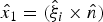 $\hat x_1 = (\hat \xi _i \times \hat n)$, which points along the negative v i direction [see Fig. 2(b)]. Then for the vector field defined in Eq. (11), Eq. (8) gives
 $$\eqalign{\dot {\vec \rho} _{\bi i} & = - \displaystyle{{\partial (\rho _i v_i )} \over {\partial x_2}} \hat x_1 + \displaystyle{{\partial (\rho _i v_i )} \over {\partial x_1}} \hat x_2 \cr & = - \rho _i \; \displaystyle{{dv_i} \over {d\xi _i}} (\hat \xi _i \times \hat n) - v_i \; \rho _i {\rm ^{\prime}}(r_i {\rm ^{\prime}})\displaystyle{{\partial r_i {\rm ^{\prime}}} \over {\partial x_2}} (\hat \xi _i \times \hat n) \cr & \quad - \rho _i \displaystyle{{\partial v_i} \over {\partial x_1}} \hat \xi _i - v_i \; \rho _i {\rm ^{\prime}}(r_i {\rm ^{\prime}})\; \hat \xi _i,} $$
since x 2 = ξ i, which is the coordinate along the dislocation line, and  $x_1 = - r_i {\rm ^{\prime}}$. It is important to note that the ∂/∂x 1 and ∂/∂x 2 operators in Eq. (14) involve displacing the field point
 $\vec r$ by either ∂x 1 or ∂x 2 along
 $\hat x_1 $ or
 $\hat x_2 $, respectively, while the dislocation stays stationary. Hence, v i being the velocity of the dislocation is independent of the position of the field point
 $\vec r$ along
 $r_i^{\prime} $, and so in Eq. (14), ∂v i/∂x 1 = 0. For the
 $\partial r_i {\rm ^{\prime}}/\partial x_2 $ term, we consider the general case of the dislocation exhibiting a local radius of curvature R. From geometry shown in Fig. 2(b), if the field point
 $\vec r$ moves by ∂x 2 along
 $\hat x_2 $, the resultant change
 $\partial r_i {\rm ^{\prime}}$ in the perpendicular distance to the dislocation
 $r_i {\rm ^{\prime}}$ is given by
 $$\eqalign{R - (r_i {\rm ^{\prime}} + \partial r_i {\rm ^{\prime}}) & = \sqrt {(R - r_i {\rm ^{\prime}})^2 + \partial x_2^2}, \;{\rm or}\;\displaystyle{{\partial r_i {\rm ^{\prime}}} \over {\partial x_2}} \cr & = \displaystyle{{ - \partial x_2} \over {\sqrt {(R - r_i {\rm ^{\prime}})^2 + \partial x_2^2} + (R - r_i {\rm ^{\prime}})}}\;.} $$
(a) Discrete dislocation i on slip plane (plane of this paper). A general field point  $\vec r\;$ is at perpendicular (shortest) distance
 $r_i {\rm ^{\prime}}$ from the dislocation line.
 $\vec r_i $ is the point on the dislocation line that is nearest to the field point
 $\vec r$. Slip plane normal
 $\hat n = \hat s \times \hat e$ (i.e., pointing out of the plane of paper). (b) Displacing the field point by ∂x 2 along the local dislocation direction
 $\hat \xi _i $ results in change in
 $r_i {\rm ^{\prime}}$ by
 $\partial r_i {\rm ^{\prime}}$ as shown.

Thus, unless  $r_i {\rm ^{\prime}} = R$, i.e., the field point
 $\vec r$ is at the center of curvature that would certainly be problematic,
 $\partial r_i {\rm ^{\prime}}/\partial x_2 = 0$. Therefore, Eq. (14) becomes
 $$\dot {\vec \rho} _{\bi i} = - \rho _i \; \displaystyle{{dv_i} \over {d\xi _i}} (\hat \xi _i \times \hat n) - v_i \; \rho _i {\rm ^{\prime}}(r_i {\rm ^{\prime}})\; \hat \xi _i. $$
Furthermore, from Fig. 2(a),  $(dv_i /d\xi _i )(\hat \xi _i \times \hat n) = -{\hat{\dot \theta}}_i (\hat \xi _i \times \hat n) = - \dot {\hat \xi} _i $, and so the above equation becomes
 $$\dot {\vec \rho} _{\bi i} = \rho _i \; \dot {\hat \xi} _i - v_i \; \rho _i^{\prime} \; \hat \xi _i, $$
which is Eq. (13). Hence,  $\vec \rho _i (\vec r)$ defined in Eq. (11) or (12) satisfies Eq. (7) and is a valid representation of the density field of a general dislocation. Moreover, Eq. (13) gives the time evolution of the dislocation-density field, and when cast in this form, the evolution does not contain the curvature as an explicit variable, as in the case of CDD.[Reference Hochrainer, Zaiser and Gumbsch4] The local curvature does affect the velocity v i due to line tension effects, but this would be a dynamics consideration rather than a kinematics one.
We further analyze the two terms in Eq. (13). The second term in Eq. (13),  $\rho _i (r_i {\rm ^{\prime}})\; \dot {\hat \xi} _i $, is obviously the change due to tilting of the dislocation on the slip plane when it is already at the field point
 $\vec r$ [so that
 $\rho _i (r_i {\rm ^{\prime}})$ is non-zero]. The first term
 $ - v_i \; \rho _i {\rm ^{\prime}}\; \hat \xi _i $ is due to the approach of the dislocation toward the field point
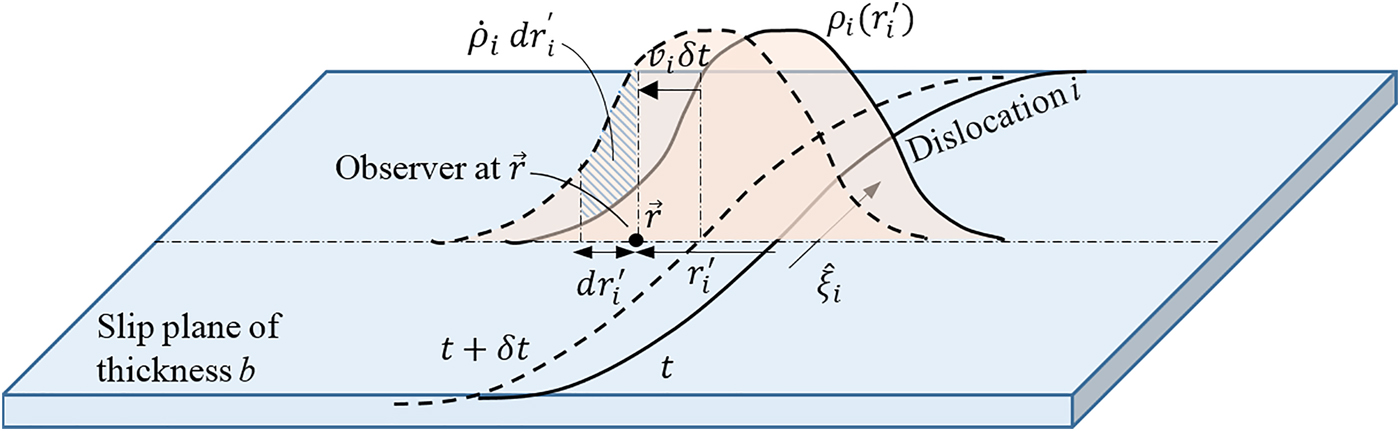
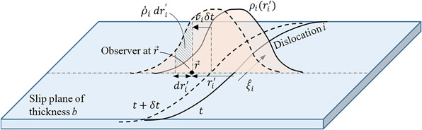
 $\vec r$. To see this, consider Fig. 3. The definition of ρ i, as quantity of dislocation threading unit plane perpendicular to dislocation line, is such that
 $b\rho _i \; dr_i {\rm ^{\prime}}$ is the quantity of dislocation within a small distance
 $dr_i {\rm ^{\prime}}$ on the slip plane, the thickness of which is b. During time δt, the quantity of dislocation that has passed through the point r′ from the dislocation
 $$= b\int_{r_i {\rm ^{\prime}}}^{r_i {\rm ^{\prime}} - v_i \; \delta t} {\rho _i (r^{\prime})\; dr^{\prime} = b\rho _i (r_i {\rm ^{\prime}})v_i \; \delta t}, $$
and the quantity of dislocation that has passed through the point  $r_i {\rm ^{\prime}} + dr_i {\rm ^{\prime}}$ from the dislocation
 $$= b\rho _i (r_i {\rm ^{\prime}} + dr_i {\rm ^{\prime}})v_i \; \delta t\;. $$
A dislocation approaching a field point  $\vec r$ with speed v i, causing the dislocation density there to increase at a rate of
 $\dot \rho _i $.
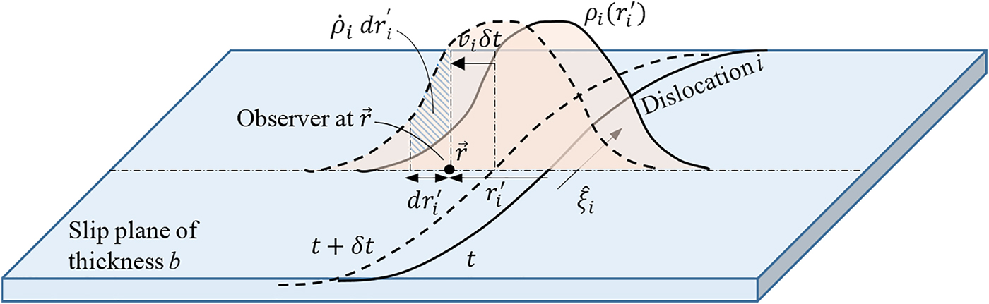
The increase in dislocation quantity between  $r_i {\rm ^{\prime}}$ and
 $r_i {\rm ^{\prime}} + dr_i {\rm ^{\prime}}$ is therefore
 $$b\; \dot \rho _i \; \delta t\; dr_i {\rm ^{\prime}} = b\; v_i \; \delta t\; [\rho _i (r_i {\rm ^{\prime}}) - \rho _i (r_i {\rm ^{\prime}} + dr_i {\rm ^{\prime}})]$$
or
 $$\dot \rho _i = - v_i \; \rho _i {\rm ^{\prime}}(r_i {\rm ^{\prime}}).$$
This increase in dislocation quantity at  $r_i {\rm ^{\prime}}$ all bears the line direction
 $\hat \xi _i $, and so the corresponding change in the dislocation-density vector at
 $r_i {\rm ^{\prime}}$ is
 $\dot {\vec \rho} _{\bi i} = - \rho _i {\rm ^{\prime}}(r_i {\rm ^{\prime}})v_i \; \hat \xi _i $, which is actually the first term in Eq. (13). It is also easy to see that, since
 $\dot {\hat \xi} _i \cdot \hat \xi _i = \dot \theta _i (\sin \theta _i \hat s - \cos \theta _i \hat e) \cdot (\sin \theta _i \hat e + \cos \theta _i \hat s) = 0$, the two terms in Eq. (13) are orthogonal to one another, with the approach and tilting term parallel and normal to
 $\hat \xi _i $, respectively.
Kinematics of coarse-grained dislocation distribution on a single slip plane
In Fig. 3, the  $\rho _i (r_i {\rm ^{\prime}})$ function for a discrete dislocation i does not change shape as the dislocation moves with velocity v i. When attempting to generalize to a coarse-grained distribution of dislocations of the same slip system, the contents of the distribution may move with different speeds, so that the overall profile may change shape; therefore, Eq. (13) is not applicable to the coarse-grained picture by simply replacing the
 $\rho _i (r_i {\rm ^{\prime}})$ thereby ρ(r′) for the coarse-grained distribution. For the coarse-grained case, we have to go back to the more general form in Eq. (7):
 $\dot {\vec \rho} = - \vec \nabla \times (\rho v\; \hat n)$. However, using this equation, or the original forms in Eq. (3) or (4), to represent a coarse-grained distribution in a straight-forward way would have the SSD components lost. To preserve the SSD contents, the evolution of each character
 $\hat \xi _\theta = \sin \theta \hat e + \cos \theta \hat s$ of the dislocation distribution has to be known, and this is the purpose here.
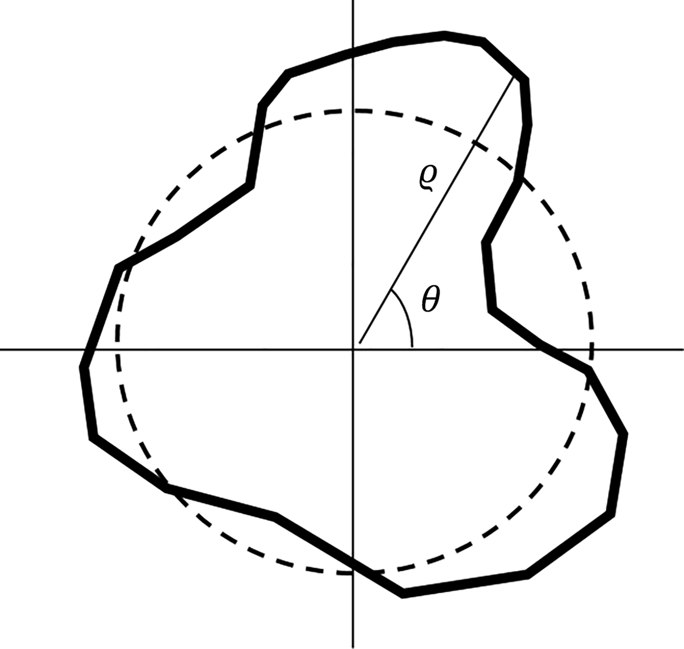
Let  $\varrho (\vec r,\theta )$ be the density of dislocations with character
 $\hat \xi _\theta = \sin \theta \hat e + \cos \theta \hat s$ at point
 $\vec r$, 0 ≤ θ ≤ 2π (Fig. 4). Specifically,
 $\varrho (\vec r,\theta )d\theta $ gives the density of dislocations of character θ to θ + dθ at point
 $\vec r$. Through
 $\varrho (\vec r,\theta )$, each character component of the total dislocation distribution is known, so
 $\varrho (\vec r,\theta )$ serves the important role of preserving the SSD contents. Without loss of generality, consider the contribution of only dislocations with character θ to the change in the dislocation-density vector
 $\vec \rho $ at a particular field point. Choosing the coordinate system to be
 $\hat x_2 = \hat \xi _\theta $, and
 $\hat x_1 = \hat \xi _\theta \times \hat n$, Eq. (10) gives this contribution as
 $$\eqalign{\left. {\dot {\vec \rho}} \right \vert _\theta & = - \displaystyle{{\partial (\varrho v)} \over {\partial x_2}} \hat x_1 + \displaystyle{{\partial (\varrho v)} \over {\partial x_1}} \hat x_2 = - \varrho \displaystyle{{dv} \over {d\xi _\theta}} (\hat \xi _\theta \times \hat n) \cr & \quad \, - v\displaystyle{{\partial \varrho} \over {\partial \xi _\theta}} (\hat \xi _\theta \times \hat n) + \displaystyle{{\partial (\varrho v)} \over {\partial x_1}} \hat \xi _\theta,} $$
where ξ θ is the coordinate along  $\hat \xi _\theta $. By the same consideration as in Fig. 2(b), ∂ϱ/∂ξ θ = 0, and by defining
 $r_{\hat \theta} = - x_1 $, which points along the
 $\vec v$ direction [and hence the opposite
 $\hat x_1 $ direction
 $\hat \theta = \hat n \times \hat \xi _\theta $, or circumferential direction in the positive sense of θ, see Eq. (6)], and writing dv/dξ θ as v θ, which represents the speed of tilting of the dislocation density, the above equation reduces to
 $$\eqalign{& \left. {\dot {\vec \rho} } \right \vert _\theta (\vec r) = - \displaystyle{{\partial (\varrho v)} \over {\partial r_{\hat \theta}}} \hat \xi _\theta - \varrho (\vec r,\theta )\; v_\theta \; (\hat \xi _\theta \times \hat n). \cr & \quad \quad \quad \quad {\rm movement}\quad \quad \quad {\rm tilting}} $$
Polar plot of the dislocation density ϱ at a given field point  $\vec r$, showing the dislocation character (θ) dependence of the density.

This equation gives the change in the dislocation-density vector  $\vec \rho $ at
 $\vec r$, due to the movement of dislocations of character θ toward and away from
 $\vec r$ (the movement term), and the tilting of dislocations initially with character θ already situated at
 $\vec r$ (the tilting term). As explained above, the purpose here is not to sum the
 $\left. {\dot {\vec \rho} } \right\vert_\theta $ in Eq. (15) over all θ, since if this is done, the resultant would only be a change in the GND at
 $\vec r$ with the SSD contents lost. Instead, we note that
 $\left. {\dot {\vec \rho} } \right\vert_\theta (\vec r)$ corresponds to the change in ϱ itself at θ. The movement term in Eq. (15) is easy to see—this term brings in, or takes away, dislocation contents with line direction
 $\hat \xi _\theta $ to or from
 $\vec r$, and so this results in a change in ϱ at θ due to dislocation movements. Writing
 $$\dot \varrho = \dot \varrho ^{{\rm move}} + \dot \varrho ^{{\rm tilt}}, $$
we have, from the first term in Eq. (15),
 $$\dot \varrho ^{{\rm move}} = - \displaystyle{{\partial (\varrho v)} \over {\partial r_{\hat \theta}}}. $$
The tilting term  $\dot \varrho ^{{\rm tilt}} $ in Eq. (16) arises from the second term in Eq. (15), but in a less obvious way. The tilting term in Eq. (15) says that the θ content of dislocations at
 $\vec r$ will be lost at a rate
 $\varrho (\vec r,\theta )\; \left. {v_\theta } \right\vert_\theta $ due to dislocations of character θ rotating to a higher angle. However, applying Eq. (15) to the character θ − dθ would give
 $\varrho (\vec r,\theta - d\theta )\; \left. {v_\theta } \right\vert_{\theta - d\theta} \; $ as a rate of gain of the θ content of dislocations at
 $\vec r$, due to rotation of dislocations with an initially lower character now to θ. Hence, during time δt, the total change in the θ content of dislocations at
 $\vec r$ due to rotation is
 $\delta \varrho ^{{\rm tilt}} d\theta = - \varrho (\vec r,\theta )\; \left. {v_\theta } \right\vert_\theta \,\delta t + \varrho (\vec r,\theta - d\theta )\; \left. {v_\theta } \right\vert_{\theta - d\theta} \,\delta t$, and so
 $$\dot \varrho ^{{\rm tilt}} = - \displaystyle{{\partial (\varrho v_\theta )} \over {\partial \theta}}. $$
The resultant evolution equation for  $\varrho (\vec r,\theta )$ is therefore
 $$\eqalign{& \dot \varrho (\vec r,\theta ) = - \displaystyle{{\partial (\varrho v)} \over {\partial r_{\hat \theta}}} - \displaystyle{{\partial (\varrho v_\theta )} \over {\partial \theta}}. \cr & \quad \quad \quad \quad {\rm movement}\quad {\rm tilting}} $$
Here, as explained before, for a given θ of the dislocation character space,  $r_{\hat \theta} $ is the coordinate along
 $\hat \theta = \hat n \times \hat \xi _\theta $, which is the circumferential direction in the positive sense of θ on the slip plane.
Instead of using Eq. (7), there is an independent way of proving Eq. (19), involving a density-distribution function for single dislocations of a similar nature as Eq. (11). Rather than specifying the density field of a single dislocation as a vector field as in Eq. (11), we may also specify it in terms of a  $\varrho (\vec r,\theta )$ function, which is now a scalar field for the dislocation density of character θ at location
 $\vec r$. Thus, for a single dislocation i as shown in Fig. 2(a), the ϱ-field may be defined as:
 $$\varrho _i (\vec r,\theta ) = \displaystyle{{\delta (r_i {\rm ^{\prime}})} \over b}\displaystyle{{\delta (\theta _i {\rm ^{\prime}})} \over {2\pi}}, $$
where  $r_i {\rm ^{\prime}}$ is the shortest distance of the dislocation from the field point
 $\vec r$,
 $\theta _i {\rm ^{\prime}} = \theta - \theta _i $ with θ i being the angular character of the dislocation at the point
 $\vec r_i $, which is nearest to the field point
 $\vec r$, and δ(x) is a δ-like function of a scalar variable x. Like Eq. (11), Eq. (20) says that ϱ i is zero everywhere on the slip plane except when the field point
 $\vec r$ is on the dislocation line, and when this is the case, ϱ i will still be zero unless θ equals the local dislocation character θ i. Thus, over the
 $(\vec r,\theta )$ space, non-zero counts of ϱ i register the locations and local characters of dislocation i.
The time evolution of ϱ i at given  $(\vec r,\theta )$ due to movement of the dislocation on the slip plane is given by differentiating Eq. (20) with respect to time at fixed
 $(\vec r,\theta )$:
 $$\eqalign{\left. {\dot \varrho _i} \right \vert _{(\vec r,\theta )} & = \displaystyle{{\delta (\theta _i {\rm ^{\prime}})} \over {2\pi b}}\delta ^{\prime}(r_i {\rm ^{\prime}})\displaystyle{{\partial r_i {\rm ^{\prime}}} \over {\partial t}} + \displaystyle{{\delta (r_i {\rm ^{\prime}})} \over {2\pi b}}\delta ^{\prime}(\theta _i {\rm ^{\prime}})\displaystyle{{\partial \theta _i {\rm ^{\prime}}} \over {\partial t}} \cr & = \displaystyle{{\delta (\theta _i {\rm ^{\prime}})} \over {2\pi b}}\delta ^{\prime}(r_i {\rm ^{\prime}})\displaystyle{{\partial r_i {\rm ^{\prime}}} \over {\partial t}} - \displaystyle{{\delta (r_i {\rm ^{\prime}})} \over {2\pi b}}\delta ^{\prime}(\theta _i {\rm ^{\prime}})\dot \theta _i.} $$
By defining  $v_i = - \partial r_i {\rm ^{\prime}}/\partial t$ as the speed of approach of the dislocation toward
 $\vec r$ as before, this becomes
 $$\eqalign{& \dot \varrho _i (\vec r,\theta ) = - \displaystyle{{\delta (\theta _i {\rm ^{\prime}})} \over {2\pi b}}v_i \; \delta ^{\prime}(r_i {\rm ^{\prime}}) - \displaystyle{{\delta (r_i {\rm ^{\prime}})} \over {2\pi b}}\dot \theta _i \; \delta ^{\prime}(\theta _i {\rm ^{\prime}}). \cr & \quad \quad \quad \quad \quad {\rm approach}\quad \quad \quad \quad {\rm tilting}} $$
When there are many dislocations moving on the slip plane, the total dislocation-density function  $\varrho (\vec r,\theta )$, and its flux quantities ϱ v and ϱ v θ can be defined as the sum of contributions of
 $\varrho _i (\vec r,\theta )$ in Eq. (20):
 $$\varrho (\vec r,\theta ) = \mathop \sum \limits_i \varrho _i (\vec r,\theta ) = \displaystyle{1 \over {2\pi b}}\mathop \sum \limits_i \delta (r_i {\rm ^{\prime}})\delta (\theta _i {\rm ^{\prime}}),$$
 $$\varrho v(\vec r,\theta ) = \mathop \sum \limits_i \; v_i \; \varrho _i (\vec r,\theta ) = \displaystyle{1 \over {2\pi b}}\mathop \sum \limits_i \; v_i \; \delta (r_i {\rm ^{\prime}})\delta (\theta _i {\rm ^{\prime}}),$$
 $$\varrho v_\theta (\vec r,\theta ) = \mathop \sum \limits_i \dot \theta _i \; \varrho _i (\vec r,\theta ) = \displaystyle{1 \over {2\pi b}}\mathop \sum \limits_i \dot \theta _i \; \delta (r_i {\rm ^{\prime}})\delta (\theta _i {\rm ^{\prime}}).$$
It should be noted that the summations in these equations do not cancel out the SSD contents, since, for example, a dislocation dipole at the same field point  $\vec r$ would have the two members registered in two θ i values separated by π apart in
 $\delta (\theta _i {\rm ^{\prime}})$, and so their ϱ i, ϱ v, or ϱ v θ values do not cancel out. From Eqs. (21) and (22), the evolution of
 $\varrho (\vec r,\theta )$ is
 $$\eqalign{& \dot \varrho = - \mathop \sum \limits_i \left[ {\displaystyle{{\delta (\theta _i {\rm ^{\prime}})} \over {2\pi b}}v_i \; \delta ^{\prime}(r_i {\rm ^{\prime}})} \right] - \mathop \sum \limits_i \left[ {\displaystyle{{\delta (r_i {\rm ^{\prime}})} \over {2\pi b}}\dot \theta _i \; \delta ^{\prime}(\theta _i {\rm ^{\prime}})} \right], \cr & \quad \quad \quad \quad {\rm movement}\quad \quad \quad \quad {\rm tilting}} $$
and again, there is a term due to movements of dislocations, and another term due to their tilting. Furthermore, it is not difficult to see that Eq. (25) corresponds well to Eq. (19). Formally, from Eq. (23),
 $$\eqalign{\displaystyle{{\partial \varrho v} \over {\partial r_{\hat \theta}}} & = \displaystyle{1 \over {2\pi b}}\mathop \sum \limits_i \delta (\theta _i {\rm ^{\prime}})\displaystyle{{\partial [v_i \; \delta (r_i {\rm ^{\prime}})]} \over {\partial r_{\hat \theta}}} \cr & = \displaystyle{1 \over {2\pi b}}\mathop \sum \limits_i \delta (\theta _i {\rm ^{\prime}})\; v_i \; \delta ^{\prime}(r_i {\rm ^{\prime}}).} $$
Here, by virtue of the  $\delta (\theta _i {\rm ^{\prime}})$ selector,
 $\partial r_{\hat \theta} $ refers to a movement of the field point [
 $\vec r$ in Fig. 2(a)] along the
 $\hat \theta = \hat n \times \hat \xi _\theta $ or
 $r_i {\rm ^{\prime}}$ direction of those dislocations i when their θ i at the points closest to
 $\vec r$ are equal to a given θ; the second step of Eq. (26) then follows from the fact that the velocities v i of such dislocations i would not change as the field point
 $\vec r$ moves this way. Similarly, from Eq. (24),
 $$\displaystyle{{\partial \varrho v_\theta} \over {\partial \theta}} = \mathop \sum \limits_i \left[ {\displaystyle{{\delta (r_i {\rm ^{\prime}})} \over {2\pi b}}\dot \theta _i \displaystyle{{\partial \delta (\theta _i {\rm ^{\prime}})} \over {\partial \theta}}} \right] = \mathop \sum \limits_i \left[ {\displaystyle{{\delta (r_i {\rm ^{\prime}})} \over {2\pi b}}\dot \theta _i \delta {\rm ^{\prime}}(\theta _i {\rm ^{\prime}})} \right],$$
since  $\theta _i {\rm ^{\prime}} = \theta - \theta _i $ and θ i and
 $\dot \theta _i $ are independent of a change ∂θ in the character space of
 $\varrho (\vec r,\theta )$. Thus, with Eqs. (26) and (27), Eq. (25) becomes
 $$\eqalign{& \dot \varrho = - \displaystyle{{\partial \varrho v} \over {\partial r_{\hat \theta}}} - \displaystyle{{\partial \varrho v_\theta} \over {\partial \theta}}, \cr & {\rm movement}\quad {\rm tilting}} $$
which corresponds exactly to Eq. (19).
We also note that Eq. (19) can be written in the alternative form:
 $$\dot \varrho (\vec r,\theta ) = - \vec \nabla (\varrho v) \cdot \hat \theta - \displaystyle{{\partial (\varrho v_\theta )} \over {\partial \theta}}, $$
where  $\vec \nabla (\varrho v) \cdot \hat \theta $ denotes the gradient of the flux ϱ v along the positive circumferential direction
 $\hat \theta $ of a given dislocation character θ.
Compatibility with CDD
Hochrainer et al.’s CDD theory[Reference Hochrainer, Zaiser and Gumbsch4] advocates the importance of the dislocation curvature[Reference Sedláček, Kratochvil and Werner3, Reference Hochrainer, Zaiser and Gumbsch4] as a second field variable in addition to the density itself. Specifically, in CDD, the evolution equation of the dislocation density is:
 $$\dot \varrho = - \vec \nabla \cdot (\varrho \vec v) - \displaystyle{{\partial (\varrho v_\theta )} \over {\partial \theta}} + \varrho vk,$$
where k is the dislocation curvature.
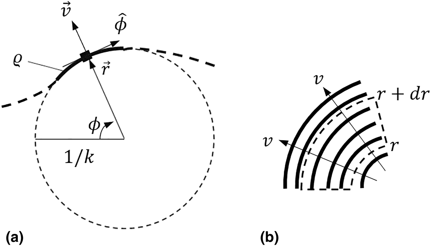
Here, we show that Eq. (30) can be recovered from Eq. (29). Consider a density of dislocations near a field point  $\vec r$ with a local curvature k there, as shown in Fig. 5(a). Without loss of generality, choose the coordinate system to be cylindrical (r, ϕ) with origin at the center of the fitting circle to the dislocation density, and unit vectors
 $\hat r$ and
 $\hat \phi $ along the radial and circumferential directions, respectively. In this case, the quantity
 $\vec \nabla (\varrho v) \cdot \hat \theta $ in Eq. (29), which is a function of
 $\vec r$ and θ, will be non-zero only when
 $\vec r = (r,\phi )$ falls on the curved dislocation, i.e., r = 1/k. Furthermore, we also have
 $\hat \theta = \hat r$, since the velocity direction of the dislocation
 $\hat v$ or
 $\hat \theta $ is simply along the radial direction
 $\hat r$ of the cylindrical coordinate [see Eq. (6) and Fig. 5(a)]. The non-zero value of
 $\vec \nabla (\varrho v) \cdot \hat \theta $ in Eq. (29) can therefore be expressed as
 $$\eqalign{\vec \nabla (\varrho v) \cdot \hat \theta & = \vec \nabla (\varrho v) \cdot \hat r = \vec \nabla \cdot (\varrho v\hat r) - (\varrho v)\; \vec \nabla \cdot \hat r \cr &= \vec \nabla \cdot (\varrho \vec v) - (\varrho v)\; \vec \nabla \cdot \hat r}$$
in which,
 $$\eqalign{\vec \nabla \cdot \hat r & = \left. {\hat r \cdot (\partial \hat r/\partial r) + (\hat \phi /r) \cdot (\partial \hat r/\partial \phi )} \right \vert _{r = 1/k} = \left. {(\hat \phi /r) \cdot \hat \phi} \right \vert _{r = 1/k} \cr & = k.}$$
(a) A density of dislocations (solid curve) at field point  $\vec r$ with local curvature k moving with velocity
 $\vec v$. (b) Uniform distribution of concentric loops expanding at the same speed.

Equation (31) therefore gives  $\vec \nabla (\varrho v) \cdot \hat \theta = \vec \nabla \cdot (\varrho \vec v) - \varrho vk$ and on substituting back to Eq. (29), Eq. (30) of the CDD theory is recovered.
Although the CDD Eq. (30) is compatible with the present Eq. (29), in the former, the dislocation density ϱ and curvature k are coupled variables solvable only with a simultaneous evolution equation for the curvature.[Reference Sedláček, Kratochvil and Werner3] However, in Eq. (29), only the variable ϱ is involved, which can be solved from that equation alone.
To further see that the curvature-generation term in the CDD is already embodied in Eq. (29), consider a simple example where an infinite series of concentric loops uniformly distributed along r are all expanding from the origin at the same speed [Fig. 5(b)]. As such loops move past a fan-shaped control volume as shown in Fig. 5(b), the averaged dislocation density ρ, i.e., number of dislocations threading unit area perpendicular to the dislocation line [see Eqs. (1) and (2)], is a constant function of R, but since the arc length at r + dr is longer than that at R, the total line length of dislocations arriving at the (r + dr) boundary of the fan-shaped control volume is longer than that at R. Therefore, in the CDD Eq. (30),  $\vec \nabla \cdot (\rho \vec v) \gt 0$, but since ρ is constant inside the control volume, the generation term ρvk has to be there to compensate. Alternatively, the fact that
 $\dot \rho = 0$ over the slip plane (except at the origin) can be embodied in a much simpler way by considering one-dimensional (1D) flux divergence
 $\vec \nabla (\varrho v) \cdot \hat \theta $ along the
 $\vec v$ or
 $\hat \theta $ direction of the dislocations as in Eq. (29). Thus, in Fig. 5(b), if we count the arrival and departure of dislocations along any 1D radial direction, rather than across the 2D fan-shaped control volume shown, then the ρ sampled at r would be the same as that sampled at r + dr, and so
 $\partial (\rho v)/\partial r = \vec \nabla (\varrho v) \cdot \hat \theta = 0$, leaving no need for an extra generation term even though there is dislocation curvature.
Discussion and conclusion
To summarize, in this work we have shown that an evolution equation for the dislocation character-specific density  $\varrho (\vec r,\theta )$ is Eq. (29), i.e.,
 $$\eqalign{& \dot \varrho (\vec r,\theta ) = - \vec \nabla (\varrho v) \cdot \hat \theta - \displaystyle{{\partial (\varrho \; v_\theta )} \over {\partial \theta}}. \cr & \quad \quad \quad \quad {\rm movement}\quad {\rm tilting}} $$
Here, v is the dislocation velocity, v θ the rotational speed of the dislocation, and  $\hat \theta $ is the unit vector along the circumferential direction in the positive sense of θ on the slip plane. To close the problem, the dislocation velocity v needs to be evaluated from a known or assumed velocity law involving the effective glide stress, which is the net of the applied stress, Peierls stress and elastic interactions between dislocation densities in the system.[Reference Leung and Ngan7] Once the v field is known, the rotational velocity can be evaluated as v θ = dv/dξ θ, where ξ θ is the dislocation line direction for a given character θ. Equation (29) describes the evolution of dislocation density of each dislocation character θ, and hence it is much more comprehensive than Eq. (4), which is for the GNDs only, or Acharya and Roy's Eq. (10)[Reference Acharya and Roy8] in which the evolution of the SSD term L p is not exactly known. Compared with the CDD,[Reference Hochrainer, Zaiser and Gumbsch4] Eq. (29) does not involve the dislocation curvature as a coupled variable. Eq. (29) is also very simple to understand—the first term describes the coming and going of dislocations of the given dislocation character to and from the field point
 $\vec r$ along the dislocation velocity direction, which is
 $\hat \theta $, while the second term describes the tilting of the dislocations away from the given dislocation character. Equation (29) is fully consistent with both Acharya's Eq. (5) and the CDD theory in Eq. (30), and so through it, the latter two theories are also shown to be compatible with each other. Future work should focus on numerically implementing Eq. (29) for the computation of real dislocation dynamics problems.
Acknowledgment
The work described in this paper is supported by Kingboard Endowed Professorship in Materials Engineering and Seed Fund for Basic Research (Project code: 201411159129) at the University of Hong Kong. This Research Letter was invited by Editor of MRS Communications, based on an invited presentation at 2017 MRS Spring Meeting.