2 Description of the problem

In this section, we formulate the problem (see [Reference Makino, Iwata, Shinohara, Jitsumatsu, Hotta, San and Aihara4, Reference Shinohara and Kobayashi7] for more information).

Let $\beta \in (1, 2)$ . Given a real number $x \in (0, 1)$ , we are interested in converting it to a 0-1 sequence $(e_i(x))_{i\geq 1}$ (where $e_i(x) =0$ or $1$ ) such that

$$ \begin{align*} x = (\beta -1) \sum_{i=1}^{\infty} \frac{e_i(x)}{\beta^i} \end{align*} $$

holds. This expression is called the $\beta $ -expansion of x. The coefficient $(\beta -1)$ appears so that the expansion $e_i(x) \equiv 1$ corresponds to the real number 1. Note that, given x, the choice of $(e_i(x))$ is not unique in general.

Let us explain how the $\beta $ -encoders transform signals into the digits with the base $\beta $ . Let $\nu \in [1-1/\beta , 1/\beta ]$ . Suppose we have a circuit that converts a given signal of magnitude $x \in [0, 1]$ into $T(x)$ , where

$$ \begin{align*} T(x) = \begin{cases} \beta x & (x \leq \nu) \\ \beta (x-1) + 1 & (x> \nu ). \end{cases} \end{align*} $$

Note that, as $T:[0, 1] \to [0, 1]$ , we have $T^n(x) \in [0, 1]$ for any $n\geq 1$ . Let $\phi $ be the indicator function given by

$$ \begin{align*} \phi(x) = \begin{cases} 0 & (x \leq \nu) \\ 1 & (x> \nu ). \end{cases} \end{align*} $$

Then, $T(x) = \beta x -(\beta -1)\phi (x)$ . Set $d_i(x) = \phi (T^{i-1}(x))$ . We have

(2.1) $$ \begin{align} T^K(x) = \beta^K x - (\beta -1)\sum_{i=1}^{K} \beta^{K-i} d_i (x) \iff x = (\beta -1) \sum_{i=1}^{K} \frac{d_i(x)}{\beta^i} + \frac{T^K(x)}{\beta^K}. \end{align} $$

Since $|T^K(x)| \leq 1$ , we see that the sequence $(d_i(x))$ gives a $\beta $ -expansion of x by letting $K \to \infty $ . This shows that if we have a circuit described as above, then by circulating the signal around this circuit and recording $d_i(x)$ , we obtain a $\beta $ -expansion of x. This is the mechanism of the $\beta $ -encoders that we are interested in.

Now let us explain the problem we discuss. If all the digits $(d_i(x))_{i \geq 1}$ are available, then there would be no loss of information in the encoding–decoding process. However, in real-world use, only a finite number of digits $(d_i(x))_{1\leq i \leq K}$ are available (K is the number of digits that we record) and there is some loss of information. That is, given $x \in (0, 1)$ , we have its incomplete $\beta $ -expansion $(d_i(x))_{1\leq i \leq K}$ . This sequence is decoded into

(2.2) $$ \begin{align} \rho_{\beta, \nu, K} (x) = \rho(x)= (\beta - 1)\sum_{i=1}^K \frac{d_i(x)}{\beta^{i}} + \frac{\theta}{\beta^K}, \end{align} $$

where $\theta $ is some real number. The last term is an auxiliary constant added so as to decrease the loss of information on average. In this article, we assume that $\theta = 0.5$ . (For the choice of $\theta $ , see [Reference Makino, Iwata, Shinohara, Jitsumatsu, Hotta, San and Aihara4, Section 2] for more information.) We are interested in how much $\rho (x)$ differs from x on average. More precisely, we want to estimate the MSE

$$ \begin{align*} \mathrm{MSE}(\beta,\nu,K) := \int_{[0, 1]} (\rho(x) - x)^2\, dx. \end{align*} $$

It is reasonable to expect that, for fixed $\beta $ and $\nu $ , the MSE would be proportional to $\beta ^{-2K}$ (see also equation (2.3)). Thus, we are interested in estimating the calibrated MSE (abbreviated to CMSE), that is, $\mathrm {CMSE}:=\beta ^{2K}\mathrm {MSE}$ .

The direct analysis of the MSE is a difficult task for large K. The number of values of $\rho (x)$ increases exponentially rapidly and, for general $\beta $ , the points of discontinuity distribute unevenly. As such, the direct calculation of the MSEs requires much effort.

In [Reference Makino, Iwata, Shinohara, Jitsumatsu, Hotta, San and Aihara4], the concept of segments is used to analyse the MSEs. By changing the variable, the calculation of the MSEs is reduced to counting the population of intervals grouped with regard to their images under $T^{K}$ . They have some Markovian property and this reduces the cost of the calculations.

The technique introduced by Shinohara and Kobayashi [Reference Shinohara and Kobayashi7] has similar flavour. First, recall that given a piecewise $C^1$ -map $S:I \to I$ (where I denotes the unit interval $[0, 1]$ ), we have the Perron–Frobenius operator P associated to S (see [Reference Shinohara and Kobayashi7] for more information). This is a linear operator acting on the space of finite measures on I. The action of P is characterized by

$$ \begin{align*} \int f(x) P(\mu) = \int f(S(x)) \mu, \end{align*} $$

for every $L^1$ -function $f(x)$ and a finite measure $\mu $ .

For our map T, using equations (2.1)–(2.2) one can check that

$$ \begin{align*} x - \rho (x) = \beta^{-K}(T^K(x) - \theta). \end{align*} $$

Thus,

(2.3) $$ \begin{align} \mathrm{MSE} = \beta^{-2K}\int (x -\theta)^2 P^K(dx), \end{align} $$

where $dx$ denotes the Lebesgue measure. Hence, to understand the MSE, we need to understand $P^n(dx)$ . Analysis of Perron–Frobenius operators was carried out by Mori (see [Reference Mori5]). In [Reference Shinohara and Kobayashi7], assuming that $\nu = 1/\beta $ (which makes the calculation easier), we obtained an explicit formula of $\eta \,dx := \lim _{n \to \infty } P^n(dx)$ , which turns out to be the invariant measure of T (see [Reference Shinohara and Kobayashi7] for more information). Also, by the spectral analysis we can have a rigorous estimate of the difference between $\eta \,dx$ and $P^n(dx)$ for large n.

In this article, we consider the case where $\nu $ is not necessarily equal to $1/\beta $ . In the case $\nu = 1/\beta $ , the generating function of $P^n(dx)$ is tightly related to the characteristic function of the segments (see [Reference Shinohara and Kobayashi7]). In our case, it seems difficult to establish the same relationship due to the fact that $\nu \neq 1/\beta $ . Instead of dealing with segments, we use different simple functions. By introducing these functions, we can obtain the explicit formula of the invariant measure and the generating function of the Perron–Frobenius operator. We show this in the next section.

3 Generating function

Given a sequence $(A_n)_{n \geq 0}$ , its generating function is a formal power series $\sum _{k=0}^{\infty } A_k z^k$ . We assume that $A_n$ are elements of some additive group. In our case, $A_n = P^n(dx)$ (we define $A_0 = dx$ ). The purpose of considering the generating function is that sometimes we can derive a closed expression of it. Then, by investigating it, we can conclude some unexpected properties of $(A_n)$ . This strategy was demonstrated in [Reference Shinohara and Kobayashi7]. By a similar analysis, we can deduce the closed formula for our case, but it will be more involved. Put

$$ \begin{align*} s(z):=\sum_{k=0}^{\infty} P^k(dx) z^k. \end{align*} $$

We want to obtain a closed expression of $s(z)$ .

We prepare some notation. Let J denote some sub-interval of I. By $\boldsymbol {1}_{J} = \boldsymbol {1}_{J}(x)$ , we denote the characteristic function of J. Given $\alpha \in [0, 1]$ , we set $\psi _{\alpha }(x) = \boldsymbol {1}_{[0, \alpha ]} -\boldsymbol {1}_{(\alpha , 1]}$ . Note that $\boldsymbol {1}_{[0,\alpha ]} =\frac 12(\psi _{\alpha }(x) + \boldsymbol {1}_{[0,1]})$ .

We set $P_{+} = \beta \nu $ , $P_{-} = \beta \nu -(\beta -1)$ . These are the “upper” and the “lower” values of $T(\nu )$ . By $\mathrm {sgn} (x)$ , we denote the sign of x: that is, $\mathrm {sgn} (x) =1$ if $x>0$ , $\mathrm {sgn} (x) =-1$ if $x <0$ and $\mathrm {sgn} (0) =0$ .

In the following, for simplicity, we assume that $T^i(P_{\pm }) \neq \nu $ for every $i \geq 0$ . Now we are ready to state our conclusion.

Theorem 3.1. We have

(3.1) $$ \begin{align} s(z) = \frac{1}{1-{z}/{\beta}} \boldsymbol{1}_{[0, 1]} + \frac{z}{2}\frac{1}{\beta-z} \frac{\chi_{+} - \chi_{-}}{1-E_{+}+E_{-}}, \end{align} $$

where

$$ \begin{align*} \chi_{\pm} = \sum_{i=0}^{\infty} \psi_{T^i(P_{\pm})} \bigg(\frac{z}{\beta}\bigg)^i, \quad E_{\pm} = \frac{1}{2} \sum_{i=0}^{\infty} \mathrm{sgn} ( T^i(P_{\pm}) - \nu )\bigg(\frac{z}{\beta}\bigg)^{i+1}. \end{align*} $$

Owing to the limitation in the number of pages, we do not give the proof of this here. The proof is similar to that in [Reference Shinohara and Kobayashi7]. The only difference is that instead of considering the generating function of the intervals, we consider the generating function of $\psi _{\alpha }$ (see also [Reference Mori5]), that is,

$$ \begin{align*} s^{\psi_\alpha}(z) = \psi_\alpha + P(\psi_\alpha)z + \cdots + P^n(\psi_\alpha)z^n+ \cdots. \end{align*} $$

Equation (3.1) can be used to estimate $P^k(dx)$ . Recall that $P^k(dx)$ is the coefficient of $z^k$ . Then, by considering the Taylor expansion of $s(z)$ , we can deduce the formula of $P^k(dx)$ . Another interesting piece of information that we can read from equation (3.1) is the asymptotic behaviour of $P^k(dx)$ . As a rational function of z, one can see that $s(z)$ has no pole on $|z| <1$ , $z=1$ is a simple pole and there are no other poles on $|z|=1$ . The residue at $z=1$ corresponds to the limit of $P^k(dx)$ . Furthermore, by the technique given in [Reference Shinohara and Kobayashi7], it is possible to obtain the rigorous error between the invariant measure and $P^k(dx)$ . In fact, the error decays exponentially rapidly. (For more information, see [Reference Shinohara and Kobayashi7].)

Applying this for sufficiently large n, we can obtain an approximated value of $\mathrm {CMSE} (\beta , \nu , n)$ by the integral (2.3) calculated with respect to the invariant measure. We give more details in the next section.

4 Residue and invariant measure

We continue the calculation. In equation (3.1), $s(z)$ is holomorphic in the disk ${|z|<1}$ , it has a simple pole at $z=1$ and this is the only pole in $|z| \leq 1$ . The pole $z=1$ corresponds to the invariant measure. More precisely, $s(z)$ can be written as

$$ \begin{align*} \frac{A}{1-z}(\chi_{+} - \chi_{-}) + M(z), \end{align*} $$

where A is some constant and $M(z)$ is some meromorphic function which is holomorphic on some disc $|z| < 1+\varepsilon $ . Then one can deduce the following theorem.

Theorem 4.1. In the above formula,

(4.1) $$ \begin{align} A= \frac{1}{(\beta -1)+G_{+} - G_{-}} \quad \text{where } G_{\pm} = \sum_{i=1}^{\infty} \frac{T^i(P_{\pm})}{\beta^i}. \end{align} $$

The calculation is straightforward (see [Reference Shinohara and Kobayashi7]). Equations (3.1) and (4.1) give us the formula of the invariant measure $\eta \, dx = \lim _{n} P^{n}(dx)$ . In fact, if one considers the Taylor expansion of $s(z)$ , the terms from $M(z)$ decay exponentially rapidly, while the terms from the other one do not. As such, the terms from the first one gives the invariant measure.

Theorem 4.2. We have

(4.2) $$ \begin{align} \eta = \sum_{i=0}^{\infty} \frac{A}{\beta^i}(\psi_{T^i(P_+)} - \psi_{T^i(P_{-})}). \end{align} $$

Using equation (4.2), we can obtain an estimate of the MSE (in equation (2.3)). In fact, for n large, $P^n(dx)$ is close to $\eta \,dx$ . As the formula of $\eta $ in equation (4.2) is given by an infinite series which decays exponentially fast, by taking some finite terms we have an approximation of $\eta $ , which also approximates $P^n(dx)$ .

5 Numerical results

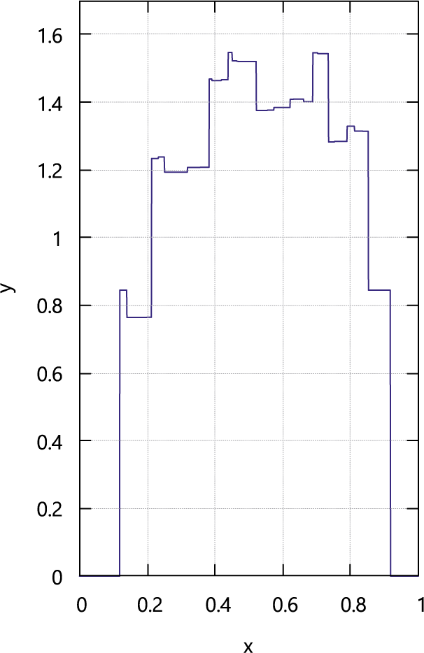
We now show the results of the previous section numerically. First, Figures 1 and 2 show the distribution function $\eta $ of the invariant measure of the map T calculated by the formula in equation (4.2). Here, x denotes the coordinate of $[0, 1]$ and y denotes the magnitude of $\eta $ .

Figure 1

The distribution function $\eta $ of the invariant measure of T, $\beta =1.8$ , $\nu =0.5$ .

Figure 2

The distribution function $\eta $ of the invariant measure of T for $\beta =1.8$ , $\nu =0.51$ .

This is a form of infinite sum of simple functions. We have drawn the graph by adding terms up to $i=20$ . We set $\beta =1.8$ , $\nu =0.5, 0.51$ , respectively. Note that, for $\nu =0.5$ , we can observe the symmetry with respect to $x=0.5$ .

Using the invariant measure, we can calculate the estimated value of the $\mathrm {CMSE}$ . Set

$$ \begin{align*} \mathrm{CMSE}^{\infty} = \int (x -\theta)^2 \, \eta \,dx. \end{align*} $$

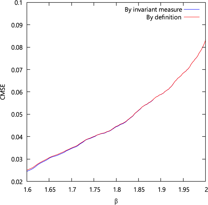
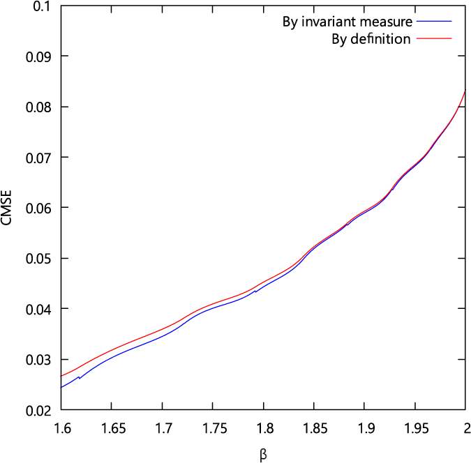
In Figures 3 and 4, we show the calculated $\mathrm {CMSE}^{\infty }$ (by the invariant measure, calculated in the same way) and compare it with the $\mathrm {CMSE} (\beta , \nu , n)$ (by definition). Recall that the $\mathrm {CMSE}$ is the $\beta ^{2K}\mathrm {MSE}$ and that the $\mathrm {CMSE}^{\infty }$ is a novel quantity which is expected to approximate the $\mathrm {CMSE}$ .

Figure 3

$\mathrm {CMSE}(\beta , 0.5, 10)$ for $1.6 \leq \beta \leq 2.0$ and $\mathrm {CMSE}^{\infty }$ .

Figure 4

$\mathrm {CMSE}(\beta , 0.5, 7)$ for $1.6 \leq \beta \leq 2.0$ and $\mathrm {CMSE}^{\infty }$ .

For $K=10$ , these two quantities are almost the same. In the range calculated, their difference is less than 3%. Note that there is some difference observable for the case $K=7$ . In the actual use of the $\beta $ -encoders, K is set around 12. Thus, for practical use, our method gives satisfactory results.

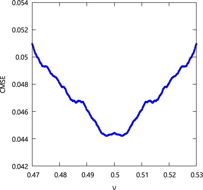
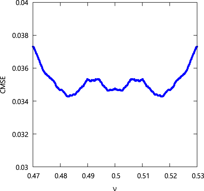
We also calculated the $\mathrm {CMSE}$ by varying the value of $\nu $ for $\beta =1.8, 1.7$ (see Figures 5 and 6). By varying $\nu $ , the $\mathrm {CMSE}$ seems to vary continuously, but it looks like it has complicated local behaviour.

Figure 5

The graph of $\mathrm {CMSE}^{\infty }$ . We set $\beta =1.8$ and $0.47\leq \nu \leq 0.53$ .

Figure 6

The graph of $\mathrm {CMSE}^{\infty }$ . We set $\beta =1.7$ and $0.47\leq \nu \leq 0.53$ .