1. INTRODUCTION
The most commonly fitted system to assist in collision avoidance in water transport is the Automatic Radar Plotting Aid (ARPA). It is aimed at assessment of the risk of collision. It is also characterised by the ability to perform so-called trial manoeuvres, enabling the navigator to see the effects of a course or a speed change that is being planned. Currently, much work on marine Collision Avoidance Systems (CAS) is focussed on the development of a CAS for application in Guidance, Navigation and Control (GNC) systems for autonomous vessels (Fossen, Reference Fossen2011). A CAS applied in a GNC system is usually a computer with an advanced optimisation algorithm for path planning and collision avoidance. Modern computational intelligence techniques are applied for this purpose, such as fuzzy logic (Mohamed-Seghir, Reference Mohamed-Seghir2014), a Collision Threat Parameters Area (CTPA) technique (Szlapczynski and Szlapczynska, Reference Szlapczynski and Szlapczynska2017), the fast marching method (Liu et al., Reference Liu, Bucknall and Zhang2017) or differential games (Lisowski, Reference Lisowski2017).
Advanced control methods, such as Linear Matrix Inequalities (LMI) (Rybczak, Reference Rybczak2018), an adaptive backstepping method (Witkowska and Śmierzchalski, Reference Witkowska and Smierzchalski2018), a fault-tolerant adaptive backstepping approach (Chen and Tan, Reference Chen and Tan2013), adaptive neural network control (Chu et al., Reference Chu, Zhu and Jan2016) or a hybrid switching controller (Tomera, Reference Tomera2017), are then applied in the motion control subsystem of the GNC system for controlling the ship in order to follow the determined path or for dynamic positioning purposes.
In a CAS for ships the following sensors are used: radars with ARPA; the Electronic Chart Display and Information System (ECDIS); the Automatic Identification System (AIS); the Global Positioning System (GPS) (or other Global Navigation Satellite System (GNSS)); speed logs and gyrocompasses. Collision avoidance manoeuvres can be performed by course and/or speed changes (speed changes are normally (but not always reductions in speed).
The algorithm applied in a CAS for ships should be characterised by compliance with the International Regulations for Preventing Collisions at Sea (COLREGs) (International Maritime Organization, 2019), simplicity, efficiency and low runtime (for near-real time application).
The research presented in this paper addresses the problem of development of a CAS for ships. The problem is solved by an appropriate collision avoidance algorithm and determining a safe manoeuvre or a safe trajectory for a ship. The method is validated by simulation tests with the use of real navigational data registered on board a ship.
The approach introduced in this paper uses a search algorithm inspired by the Artificial Potential Field (APF) method, therefore the existing APF approaches for path planning are analysed here for comparative purposes. Results of this analysis are presented in Table 1.
A summary of the most interesting APF based path planning algorithms found in recent literature.

Path planning methods for mobile robots and ships are considered. The main assumptions and operation principles of the methods are analysed. The type of obstacles taken into account during the calculation of a safe path is judged, because some methods are capable of considering only static obstacles. The method validation is also evaluated. The table specifies whether the presented results include simulations or real experiments.
It was decided to use the APF method due to the encouraging results of this method presented in the literature for mobile robot path planning problems. The advantage of this approach is its deterministic nature, which leads to the achievement of a repeatable solution for every run of the algorithm with the same input data - the same trajectory calculated in the same amount of time. The challenge of this feature is a serious limitation in heuristic methods.
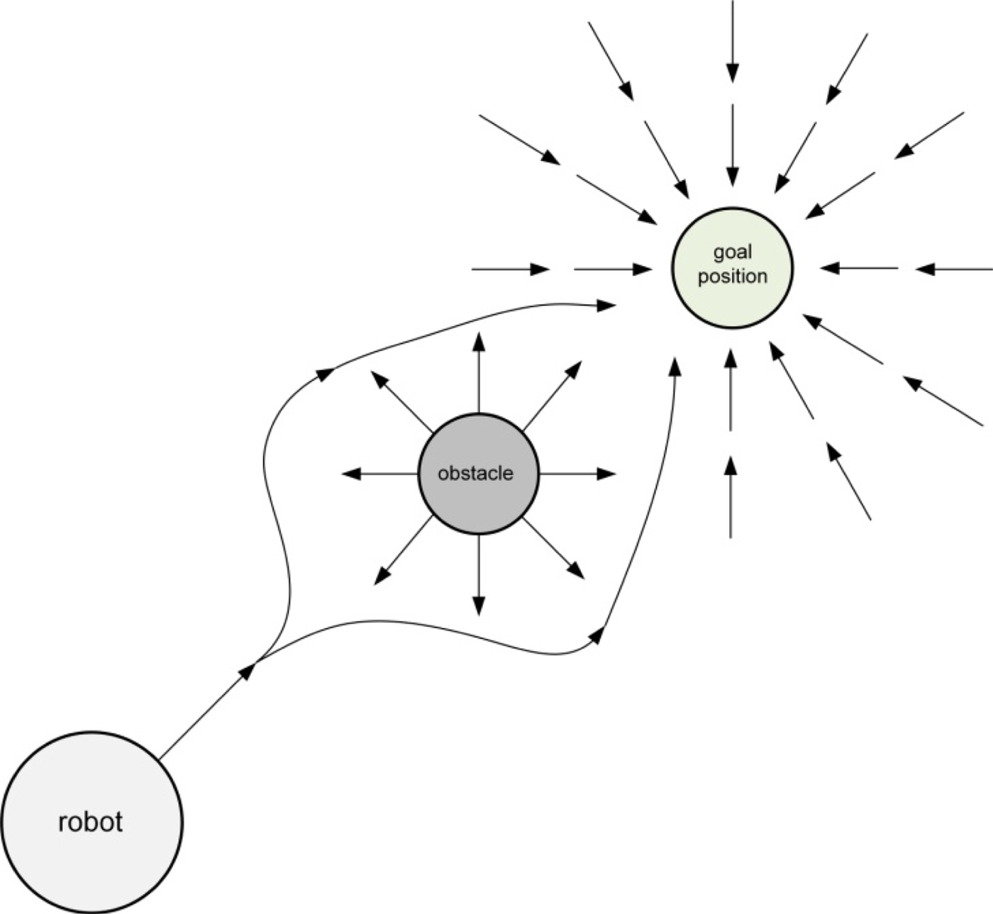
The APF method introduced by Khatib (Reference Khatib1986) is based on the concept of attractive and repulsive potential forces. The attractive potential force around the goal position pushes the moving object (a robot or a vessel) towards it, while at the same time the repulsive potential force around obstacles repels it from them, as shown in Figure 1.
The concept of the APF method.

The Potential Field Method (PFM) was proposed by Ge and Cui (Reference Ge and Cui2002) for mobile robot path planning. In this approach, potential functions take into account both the relative positions and relative velocities with respect to the target and obstacles. The method was validated by simulations and hardware experiments using small (7·5 cm × 7·5 cm × 7·5 cm) differentially driven two-wheeled mobile robots.
The Velocity Planning Potential Field method (VP PFM) was introduced by Huang (Reference Huang2009) for mobile robot path and speed planning. This also proposed a version of functions defining attractive and repulsive potentials. Its effectiveness was proven by simulation tests.
Hui and Pratihar (Reference Hui and Pratihar2009) compared a PFM for mobile robot path planning with genetic-fuzzy and genetic-neural approaches. Results of simulation studies and real experiments with a small two-wheeled robot were presented in their paper.
Valbuena and Tanner (Reference Valbuena and Tanner2012) presented a PFM for a static environment (Static PFM). This method solves a path planning problem of a nonholonomic differentially driven mobile robot by using a potential field generated by a navigation function based on the robot's position. The method was validated by simulations and real experiments with a small four-wheeled mobile robot.
The APF method has also been used in marine applications. Lee et al. (Reference Lee, Kwon and Joh2004) introduced a Modified Virtual Force Field (MVFF) method for ship's path planning. Besides the attractive force, which pulls the vessel towards the goal position (the next waypoint), in this approach an additional force is also applied for track keeping. Another force (an equivalent of a repulsive force in a classical APF method) is applied for collision avoidance. This force is determined with the use of a set of fuzzy rules. The method was verified by simulations with one moving obstacle.
Tam and Bucknall (Reference Tam and Bucknall2010) applied a Vector Field to direct the Evolutionary Algorithm (EA VF) towards the proper region of interest in the solution search process. The vector field surrounds each Safety Area around a target ship. It is called a COLREGs-influenced area and is generated taking into account the encounter situation type in order to force a proper own ship manoeuvre fulfilling the COLREGs. The difference between an own ship heading and the generated vector field was evaluated in the path's fitness function. The method was assessed by simulations with solutions calculated from perspectives of all of the ships taking part in the navigational situation considered.
Naeem et al. (Reference Naeem, Henrique and Hu2016) proposed a Modified Artificial Potential Field (MAPF) method for ship collision avoidance. In this approach, potential field functions use appropriate gain constants for obstacles and the goal. Virtual obstacles with repulsive potentials were implemented in order to receive a solution compliant with COLREGs. The method was validated by simulation studies with static and up to three dynamic obstacles (target ships).
Wang et al. (Reference Wang, Yan and Wang2017) proposed an application of a Virtual Force Field (VFF) around an own ship and target ships in order to maintain a safe distance during manoeuvres. The presented system was composed of two layers: the decision-making layer based on COLREGs and the path planning layer using the APF concept.
The main difference between the existing APF path planning approaches for mobile robots and ships and the method proposed in this paper is the method of application of a potential field. In the approaches presented in the literature a continuous potential field is created with the use of functions describing the attractive and repulsive potentials. In the proposed approach the potential field is discrete and is created with the use of a set of rules.
Most of the compared methods do not take into account static obstacles, despite the method introduced by Valbuena and Tanner (Reference Valbuena and Tanner2012), applicable for static environments and the MAPF approach proposed by Naeem et al. (Reference Naeem, Henrique and Hu2016). The proposed method is capable of solving a ship's trajectory planning problem with both static and dynamic obstacles.
In order to emphasise the difference between the proposed Discrete Artificial Potential Field (DAPF) algorithm and other existing approaches, it was decided to compare the method with the MAPF introduced by Naeem et al. (Reference Naeem, Henrique and Hu2016). The approaches were compared in terms of the most important features such as the environment representation, compliance with COLREGs the path search principle and the modelling of target ships. Table 2 presents the summary of this comparative analysis.
A comparative analysis between MAPF and DAPF.

In MAPF, a continuous environment is used, created with the use of attractive and repulsive potential functions with appropriate gains assigned, which decide the shape of the field and its contours. In DAPF a discrete environment is applied. The limited admissible solutions set is extended by the use of a Path Optimisation Algorithm (POA), which allows for achievement of an optimised collision free trajectory composed of course change manoeuvres within a broad range of values, not only those resulting from an eight-connected mapping.
In MAPF, target ships are modelled as point sources with a repulsive field around them, while in DAPF, a hexagon domain is applied around every moving obstacle, which ensures that a proper distance is maintained between an own ship and target ships during manoeuvres.
Static obstacles in MAPF are modelled taking into account only coastlines with the use of a repulsive potential field, while in DAPF both the interiors of land areas and coastlines are taken into account and modelled with the use of polygons, marked in a grid-based model as occupied and free cells.
COLREGs compliance of the calculated trajectory in MAPF is achieved by assigning virtual obstacles with repulsive fields in regions previously determined as forbidden for the own ship. In DAPF, COLREGs compliance of the calculated own ship trajectory is assured by a proper shape and size of the target ships' domains and the arrangement of the potential field.
In MAPF, the own ship safe trajectory is calculated by following the gradient of steepest descent in the potential field, which for some cases requires the trajectory to need smoothing, because constant small changes of course might not be desirable and applicable in real applications.
In DAPF, the calculated safe trajectory is then smoothed by the POA, which allows for achievement of a trajectory composed of a small number of manoeuvres, characterised by small course changes, but with values greater than 10°. This ensures compliance with COLREGs rule 8b and makes this solution applicable in real systems.
The main novelty and contributions of the presented approach include the development of:
• the Discrete Artificial Potential Field (DAPF) method to obtain a collision-free trajectory for an own ship in near-real time,
• the Path Optimisation Algorithm (POA) to achieve an optimised collision-free trajectory for an own ship in near-real time,
• the possibility to consider both static and multiple dynamic obstacles (target ships),
• methods to assure COLREGs compliance by application of a proper shape and size of a ship domain and an appropriate discrete potential field,
• a method of taking dynamic obstacles into account in the solution search process.
The remainder of this paper is organised as follows. In Section 2 a method applied in a CAS for optimised collision-free trajectory calculation is introduced. Section 3 presents results of simulation tests with real navigational data. The last section contains a summary of the paper and a proposal for future research directions.
2. METHOD
2.1 System description
A CAS for ships constitutes a subsystem of the GNC system (see Figure 2), called the Guidance System. Its aim is to calculate a safe manoeuvre or a safe trajectory for a ship based on data received from the Navigation System. The Navigation System provides information about positions, courses, speeds, distances from an own ship and bearings of the target ships detected in the environment. The aim of the Control System is to determine appropriate control forces in order to follow the safe trajectory calculated by the Guidance System.
The structure of a GNC system.

A CAS for ships has to calculate a safe trajectory between the current own ship position and a predefined final position of the ship, for example, the next waypoint. A safe trajectory is a path enabling the ship to avoid a collision with static (land, shallow water) and dynamic (target ships) obstacles. A safe trajectory has to be compliant with COLREGs and has to be calculated in, at most, a few seconds in order to fulfil the near-real time operation requirement.
The model of the process applied for calculation of a ship's safe trajectory is defined by Equations (1), where the state variables are: x1 = x, x2 = y, x2·j+1 = xj, x2·j+2 = yj, for (j = 1, …, n), n is the number of target ships tracked in the environment and x and y are coordinates of the ship's position. The decision variable u is represented by the own ship course Ψ. Target ships were assumed not to change their courses and speeds. Dynamic properties of an own ship during a course alteration manoeuvre are taken into account by the use of the manoeuvre time, defined as the time of the ship movement from the beginning of the manoeuvre to the moment when the value of the new course has been reached.
 $$\eqalign{\dot{\rm x}_1 & ={\rm V}\cdot\sin {\rm u\lpar t\rpar }={\rm V}\cdot\sin\psi{\rm \lpar t\rpar } \cr \dot{\rm x}_2 & ={\rm V}\cdot\cos {\rm u\lpar t\rpar }={\rm V}\cdot\cos\psi{\rm \lpar t\rpar } \cr \dot{\rm x}_{2\cdot {\rm j}+1} & ={\rm V}_{\rm j}\cdot\sin\psi_{\rm j}{\rm \lpar t\rpar } \cr \dot{\rm x}_{2\cdot {\rm j}+2} & ={\rm V}_{\rm j}\cdot\cos\psi_{\rm j}{\rm \lpar t\rpar }} $$
2.2. Method description
The method applied in a CAS for ships has to be simple, fast and efficient. It was decided to apply an algorithm inspired by the Artificial Potential Field (APF) method. Three major problems that have to be solved during the design of an algorithm for application in a CAS are the environment representation, the consideration of constraints and the search algorithm design.
2.2.1. The environment representation
In the presented approach an environment is represented as a grid-based map composed of m × n cells (m is the number of horizontal cells and n is the number of vertical cells). The cells are categorised as free cells, cells occupied by obstacles, a start cell and a goal cell. Every cell is characterised by the position of its centre (x and y coordinates) and a potential. Potentials are assigned to the cells according to the following rules:
• cells occupied by obstacles have a potential equal to infinity,
• a goal cell has a potential equal to zero,
• free cells are assigned with increasing potentials from goal cell to start cell according to Equation (1) (x and y are cell coordinates),
• cells on the right side from the line segment connecting the start and goal cell have lower potentials than those on the left side in order to enforce compliance with COLREGs (rules 14 and 15) (Cockcroft and Lameijer, Reference Cockcroft and Lameijer2012).
(2) $${\rm c}_{\rm xy}= \left\{\matrix{{\rm c}_{00}-10 \cdot {\rm y}\comma \; \quad {\rm x}=0\comma \; \hfill & 0 \leq {\rm y}\leq {\rm m}-1 \hfill \cr {\rm c}_{0{\rm y}}+{\rm x}\comma \; \hfill & 1 \leq {\rm x} \leq \displaystyle{{{\rm n}-1}\over{2}} \hfill \cr {\rm c}_{0{\rm y}}-{\rm x}+0{\cdot}5\comma \; \hfill & \displaystyle{{-{\rm n}-1}\over{2}}\leq {\rm x}\leq -1 \hfill \cr} \right. $$

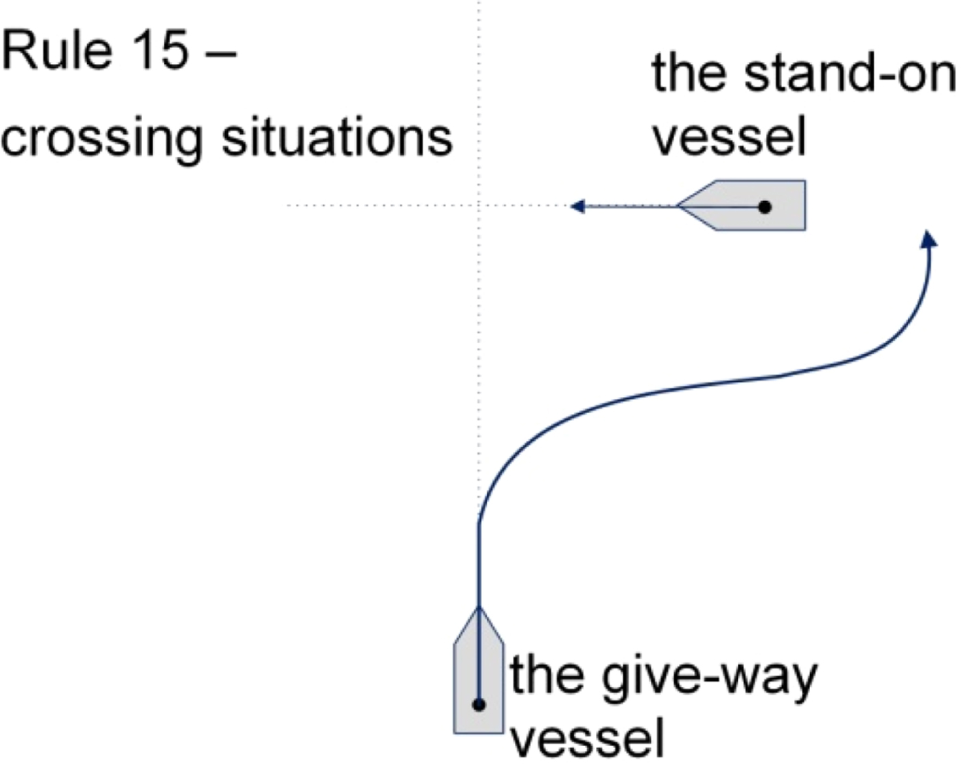
Rule 14 deals with the head-on situation. According to this rule, both vessels should alter their course to starboard (Figure 3). Rule 15 concerns the crossing situation. It states that the vessel which has the other vessel on the starboard side shall give way and if possible, avoid crossing ahead of the other ship (Figure 4).
Rule 14 of COLREGs.

Rule 15 of COLREGs.

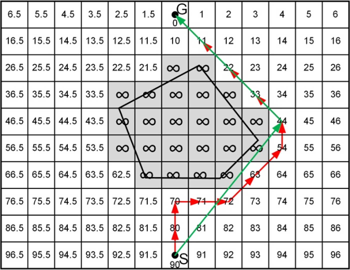
The use of the above listed rules leads to the achievement of a grid-based map constituting a discrete potential field (Figure 5), which will be used by the search algorithm to find the shortest collision-free trajectory between the start and goal cells.
A grid-based map (S - start node, G - goal node).

2.2.2. Consideration of the constraints
Static obstacles are modelled as polygons. A cell intersected by an edge of an obstacle is marked as a cell occupied by an obstacle, as shown in Figure 6. Target ships are modelled with the use of a ship domain. The ship domain is an area around a ship that constitutes a safety margin. This ensures that a safe distance between the ships will be maintained during manoeuvres.
A grid-based map (grey colour cells - cells occupied by an obstacle).

A hexagon domain, introduced by Smierzchalski and Michalewicz (Reference Smierzchalski and Michalewicz2000), was applied in the algorithm, but the approach enabled the application of other shapes of the target ship domain, for example, in a form of an ellipse, a circle or a parabola. The dimensions of the target ship domain enforce COLREGs compliance of the calculated own ship trajectory. Enlargement of the target ship domain in the bow direction forces an own ship to pass astern of the target vessel in a crossing situation (rule 15 of COLREGs). Extension of the target ship domain on the starboard side induces a course alteration of an own ship to the starboard side in a head-on situation (rule 14 of COLREGs).
Target ships are taken into account along with their motion parameters. First an intersection between the course of a target ship (a ship that has to be avoided) and the course of an own ship (a ship for which a safe trajectory is calculated) is verified. If an intersection occurs, the target ship is marked as a dangerous dynamic obstacle and is taken into account during calculation of a safe trajectory.
2.2.3. The search algorithm
The method for calculation of a collision-free trajectory for an own ship is called the Discrete Artificial Potential Field (DAPF) algorithm, because it applied the concept of an Artificial Potential Field to a discrete two-dimensional configuration space. A block diagram of the DAPF algorithm is presented in Figure 7.
A block diagram of the DAPF algorithm.

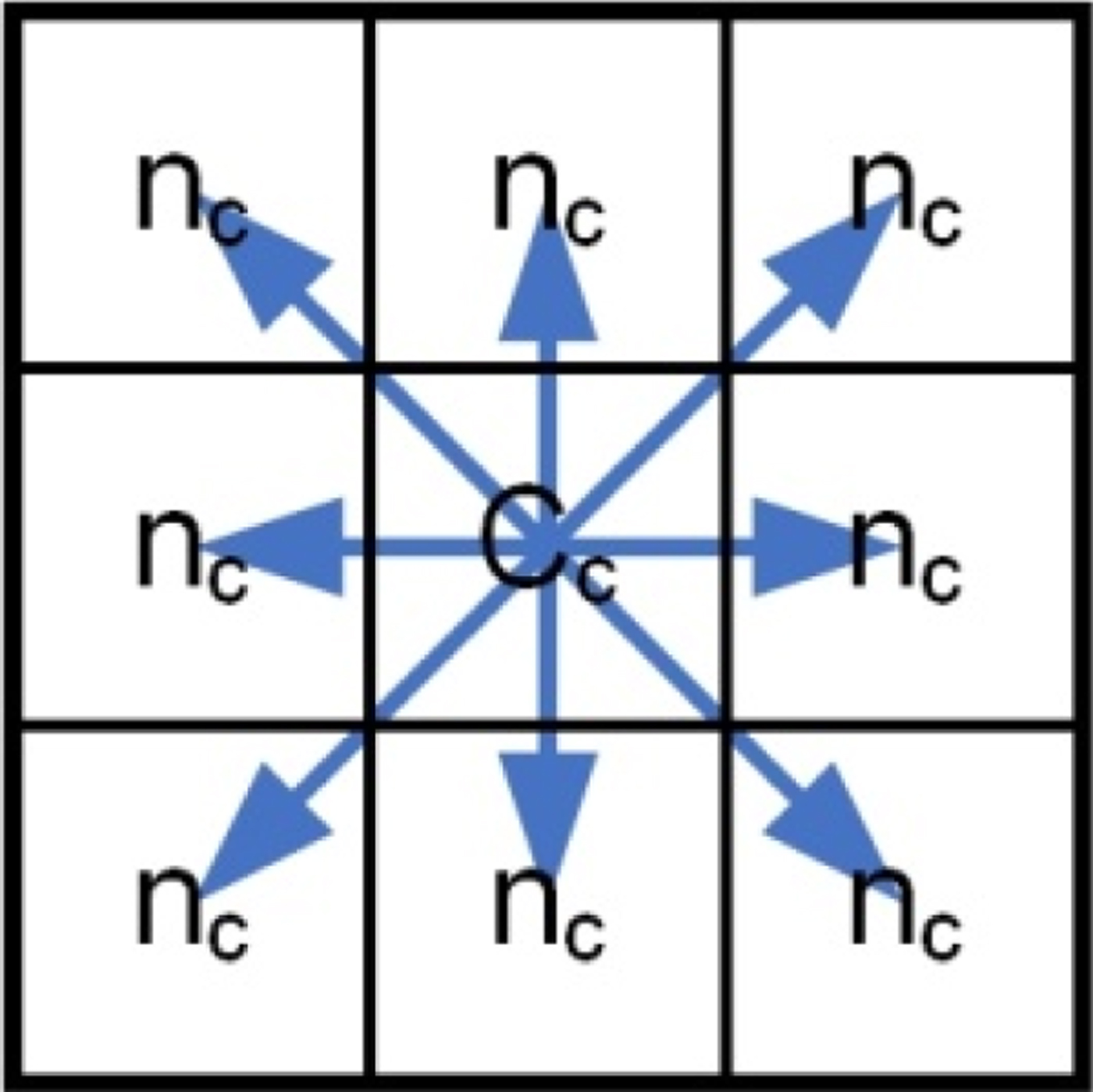
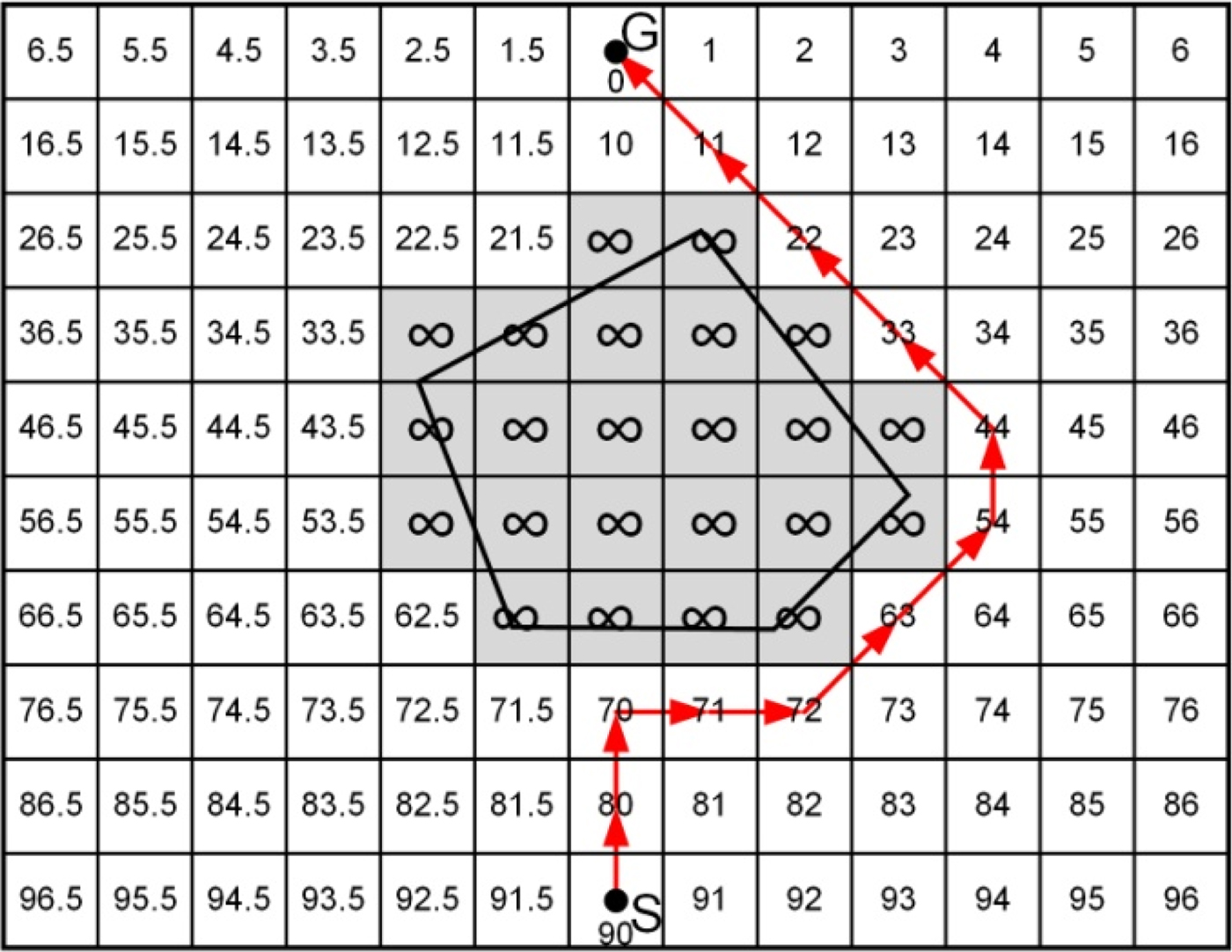
Each cell uses an eight-connected mapping, which means that from each node (centre of a cell) there are eight possibilities of movement, as shown in Figure 8. The search algorithm calculates a collision-free path for a ship by choosing, at every step, the next node (cell) with the lowest value of its potential from the neighbouring nodes, beginning from the start node. The value of the potential of every chosen cell is changed into infinity in order to prevent generation of loops in the path. The algorithm terminates when it reaches the goal node. An example of a collision-free path is shown in Figure 9.
An eight-connected mapping (cc - current cell, nc - neighbouring cell).

A collision-free path (red arrows).

2.2.4. Path optimisation
As shown in Figure 9, the path calculated by the DAPF algorithm is a collision-free path, but not the shortest path. Therefore, a Path Optimisation Algorithm (POA) is applied in order to obtain an optimised collision-free trajectory. A block diagram of the POA is given in Figure 10. The operational principle of the POA is based on an intersection check between two line segments - a line segment connecting two nodes belonging to the collision-free path checked for possibility of connection and a line segment constituting an edge of an obstacle. An example of an optimised collision-free trajectory is shown in Figure 11.
A block diagram of the POA.

A collision-free optimised path (green arrows).

A target ship hexagon domain.

The obstacles in the block diagram of the algorithm include both static and dynamic obstacles. An intersection is checked between the line segment constituting a part of a trajectory and all line segments constituting edges of static and dynamic obstacles. If an intersection is detected, further checking is stopped and the nodes connecting this line segment will not be connected. If the check does not indicate intersection, the checked line segment becomes a part of the smoothed path.
Before presentation of the final solution there is an additional check procedure, which verifies whether or not an own ship movement along the whole trajectory causes a collision with any of the target ships.
3. RESULTS
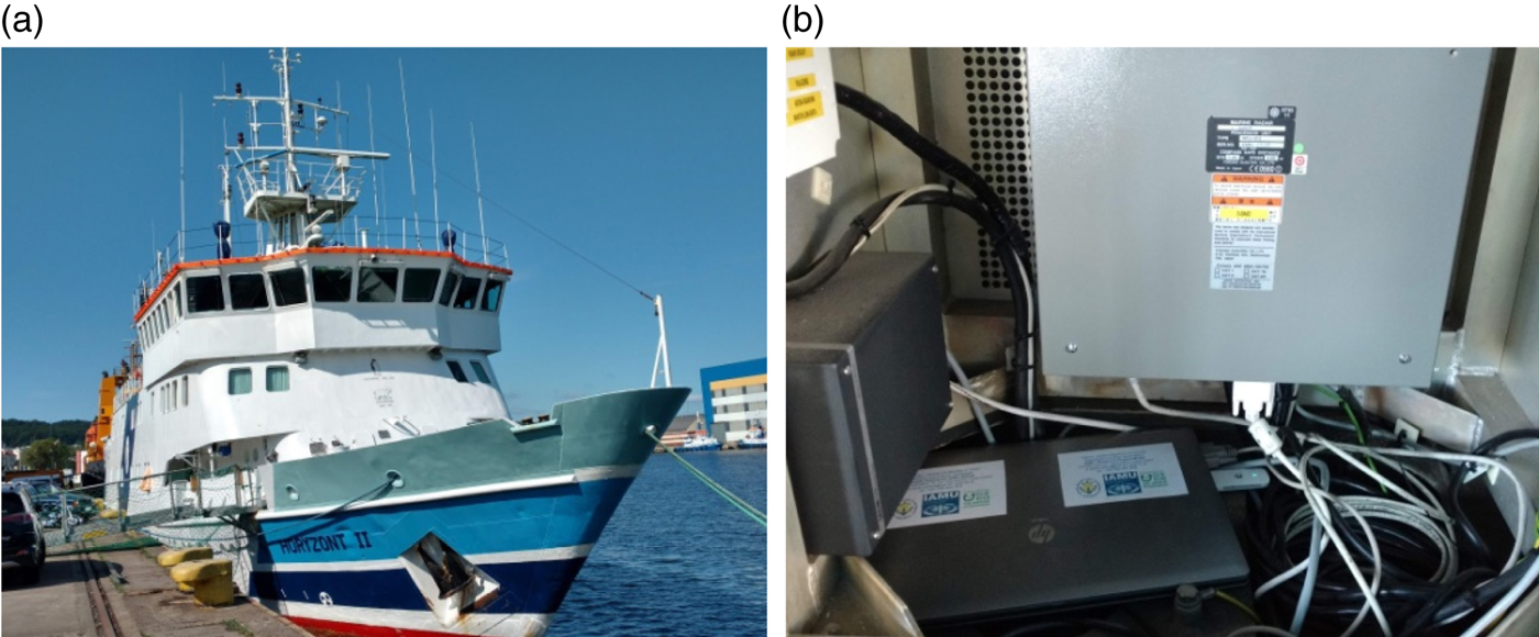
In order to validate the proposed approach, the algorithm was implemented in the MATLAB programming language and tested with the use of data from real situations registered on board the research and training ship Horyzont II. The vessel and the installation for data registration is shown in Figure 13. Input data used for example test cases are listed in Tables 3–5. The calculations were carried out with the use of a PC with an Intel Core 2 Duo E7500 2·93 GHz processor, 4 GB RAM and 64–bit Windows 7 Professional operating system. The following dimensions of the hexagon target ship domain were used for the simulation tests: A – distance towards bow = 1·0 nm, B – distance of amidships = 0·6 nm, C – distance towards starboard = 0·6 nm, D – distance towards stern = 0·25 nm, E – distance towards port side = 0·25 nm. Solutions calculated by the algorithm for example real situations are shown in Figures 14–16.
The system for real experiments: (a) the research and training ship Horyzont II (b) and the installation for registration of real collision situations.

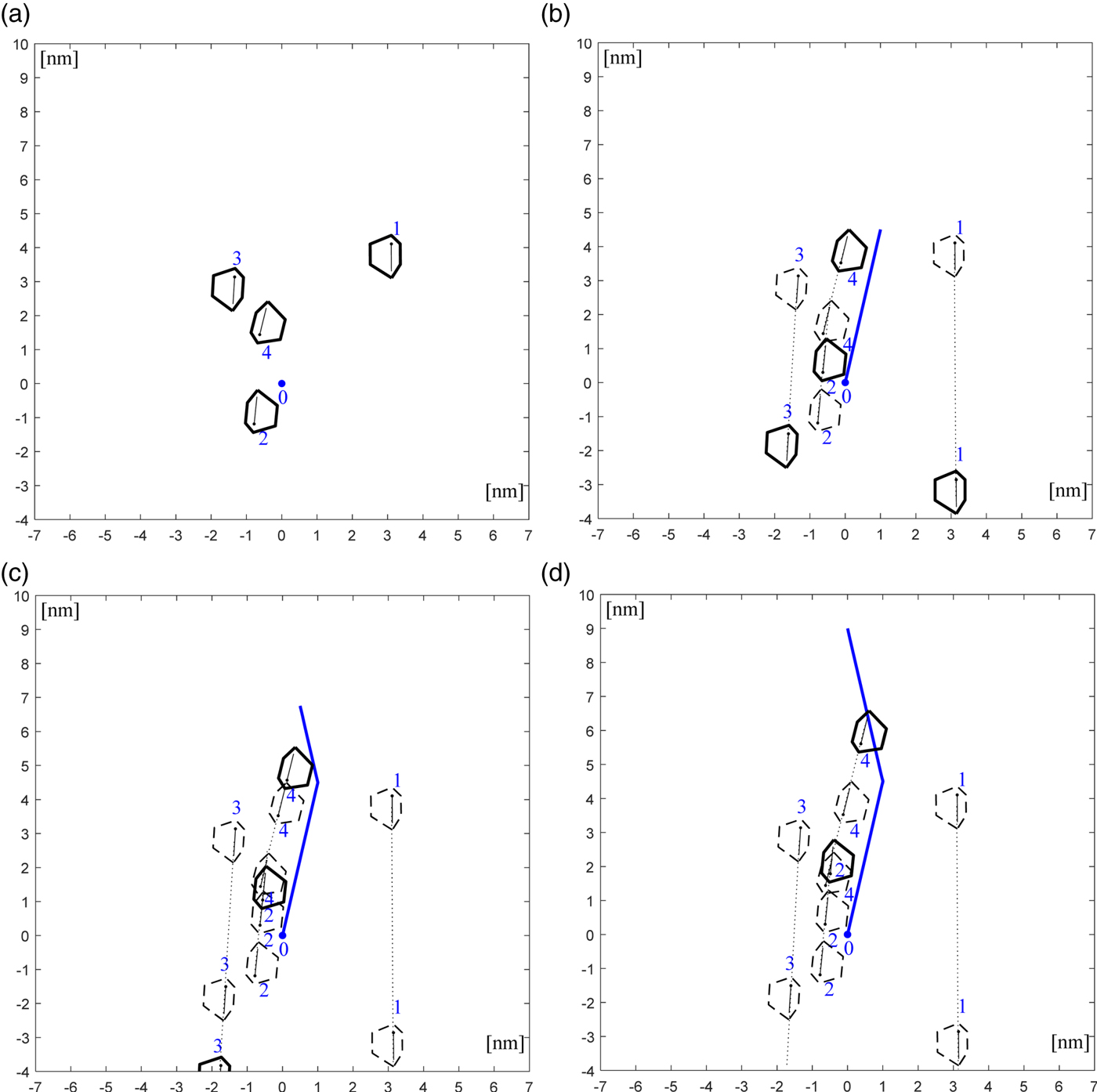
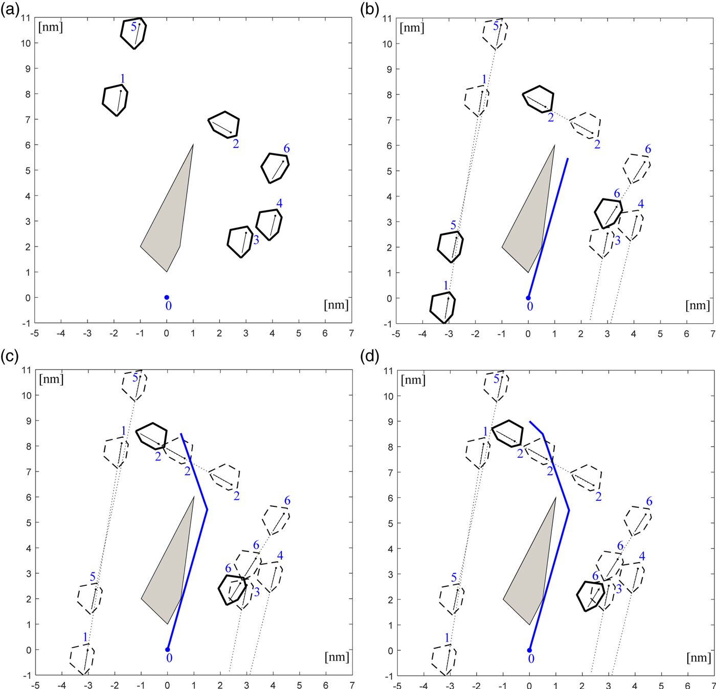
A collision-free trajectory for situation 1, run time: 0·5 s.

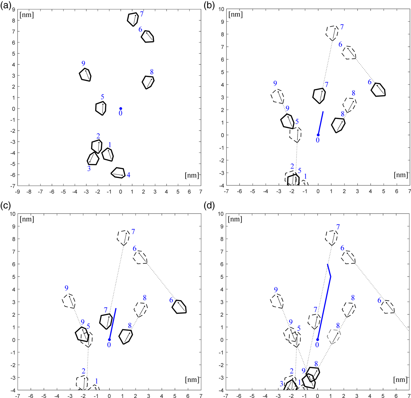
A collision-free trajectory for situation 2, run time: 0·7 s.

A collision-free trajectory for situation 3, run time: 0·45 s.

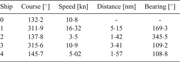
Input data for situation 1.

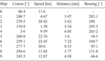
Input data for situation 2.

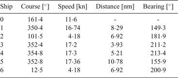
Input data for situation 3.

3.1. Navigational situation 1
The first navigational situation presents an encounter of an own ship (marked with the number zero) with four target ships marked with consecutive numbers. The input data to the algorithm is shown in Table 2. The first column presents the numbers indicating the ships as marked in Figure 14. The second column contains the courses of an own ship and the target ships in degrees, while in the third column, speeds of an own ship and target ships in knots are listed. The fourth column contains the distances to the target ships from an own ship in nautical miles. The last column lists the bearings of the target ships relative to true north in degrees.
The run time of the algorithm for this test case reached 0·5 s. Figure 14 presents the successive stages of an own ship movement along the determined trajectory. The blue line presents the calculated own ship trajectory. Figure 14(a) presents the initial phase of the navigational situation. The figure is oriented in the own ship course up orientation, which means that the own ship heading line points upwards on the graph. Figure 14(b) presents the situation when an own ship is located at the course alteration point, where it alters its course to 120°. Figure 14(c) shows the moment, in which an own ship continues its movement to the defined endpoint. Figure 14(d) shows the situation when an own ship reaches the end waypoint.
The graphical presentation of results at consecutive stages of an own ship movement confirms that the calculated own ship manoeuvres allow the avoidance of all target ships maintaining a safe distance between the ships. The values of course alterations were 13° to the starboard side and 25° to the port side, which gives acceptable compliance with rule 8b of the COLREGs. This rule states that course alterations should be large enough so they are “readily apparent to another vessel observing visually or by radar”. The solution is also compliant with rule 13 of COLREGs, dealing with the overtaking situation.
3.2 Navigational situation 2
The second navigational situation presents an encounter between an own ship and nine target ships. The input data describing this situation are listed in Table 4.
The run time of the algorithm for this situation was 0·7 s. Figure 15 presents the graphical solution of this situation. Figure 15(a) shows the initial phase. This situation is more complex than situation 1, but the algorithm found a solution for this case also composed of two course change manoeuvres. Figures 15(b)–(d) present the following stages of an own ship movement along the calculated trajectory and the corresponding positions of target ships. Own ship course alterations reached the following values: 12° to the starboard side and afterwards 26° to the port side. These values confirm the solution's compliance with rule 8b of COLREGs. The solution also fulfils rule 15 of COLREGs. According to this rule an own ship should give way to vessel number 7 and if possible, avoid crossing ahead of the other ship.
3.3. Navigational situation 3
The third navigational situation presents an encounter between an own ship and six target ships. In this situation, a static obstacle, modelling an island or a shallow area, is also present in the environment. This situation was not registered on board the ship. The aim of presenting it is to demonstrate the algorithm's capability of taking both static and dynamic obstacles into account. The input data for this situation are given in Table 5.
The run time of the algorithm for this situation was 0·45 s. Figure 16 shows the graphical solution of this situation. Figure 16(a) shows the initial phase. For this situation, the algorithm found a solution composed of three course alterations. Figure 16(b) shows the moment, when an own ship changes its course to 143°, while Figure 16(c) presents the situation, when an own ship alters its course to 116°. In Figure 16(d) the own ship is at the end waypoint. The own ship course changes for this situation were equal to: 16° to the starboard side, then 34° to the port side and finally 27° also to the port side. These results confirm the solution compliance with the rule 8b of COLREGs.
The presented results demonstrate that the algorithm calculates a collision-free trajectory in near-real time (less than a second), which makes it applicable for a marine Collision Avoidance System.
4. CONCLUSIONS
This paper presents a concept of a marine Collision Avoidance System. The algorithm developed for application in a CAS for ships is introduced. It is based on the Artificial Potential Field (APF) approach. It is applied to a discrete two-dimensional configuration space. The environment is represented as a grid-based map and a Path Optimisation Algorithm (POA) is applied in order to obtain an optimised collision-free trajectory.
Simulation studies with input data from real navigational situations registered on board the research and training ship Horyzont II validate the approach. The results demonstrate that the algorithm is capable of finding an optimised collision-free trajectory for a ship in near-real time.
The algorithm efficiently solves complex real navigational situations with multiple target ships. The solutions are compliant with the following COLREGs rules: 8b, 13, 14 and 15. Safe trajectories are optimised by the use of the POA.
To sum up, the following contributions, proving the novelty of the presented approach are:
• the development of an APF-inspired method of finding a COLREGs-compliant collision-free trajectory for an own ship in near-real time (less than a second), applicable for a commercial Collision Avoidance Systems for ships,
• a COLREGs-compliant trajectory by the use of an appropriate shape and size of a target ship domain and a suitable discrete potential field,
• a POA for optimised collision-free trajectory achievement (the shortest collision-free trajectory):
• taking into account both static and dynamic obstacles,
• taking dynamic obstacles into account in the search algorithm (determination of dangerous target ships and their proper placement),
• repeatable results for every run of calculation with the same input data,
• the calculation of an own ship trajectory to the specified final point, which enables the method to solve navigational situations in restricted waters, taking into account weather conditions (good or restricted visibility) by the change of a target ship domain size (some requirements of rule 19 of COLREGs are fulfilled).
The following limitations are also recognised:
• the speed reduction manoeuvre of an own ship has not been implemented in the current version of the algorithm,
• it is assumed that target ships do not change their courses in the solution construction process, when the target ship's course or speed change is detected, an own ship trajectory is recalculated,
• the DAPF algorithm needs data concerning free and occupied cells, therefore a bitmap would be needed as an input; however, POA needs shapes and sizes of static obstacles as input, so Electronic Nautical Chart (ENC) use would also be needed in this case.
Future research will include the implementation of the CAS system on board a ship and of carrying out of tests during voyages.