INTRODUCTION
The benthic infauna community is a key indicator of biodiversity and changes in marine environments (Feder et al., Reference Feder, Day, Jewett, McCumby, McGee and Schonberg1985; Kaiser & Spencer, Reference Kaiser and Spencer1996; Hutchings, Reference Hutchings1998; Grebmeier et al., Reference Grebmeier, Overland, Moore, Farley, Carmack, Cooper, Frey, Helle, McLaughlin and McNutt2006; Domínguez-Castanedo et al., Reference Domínguez-Castanedo, Rojas-López, Solís-Weiss, Hernández-Alcántara and Granados-Barba2007). Polychaetes are representative of the macrobenthic community, particularly as an indicator group for infauna, and have been proposed as surrogates of overall diversity because of their high abundance and functional diversity (Olsgard et al., Reference Olsgard, Brattegard and Holthe2003; Włodarska-Kowalczuk & Kędra, Reference Włodarska-Kowalczuk and Kędra2007).
Polychaetes are an important component of the marine foodweb and a necessary input for its energy budgets (Fauchald & Jumars, Reference Fauchald and Jumars1979). They constitute substantial portions of the diets of many fish, crustaceans, molluscs, marine mammals and seabirds in cold-water ecosystems (Dayton et al., Reference Dayton, Mordida and Bacon1994; Gambi et al., Reference Gambi, Castelli and Guizzardi1997; Quijón & Snelgrove, Reference Quijón and Snelgrove2005). In trawled or otherwise human-disturbed areas, polychaetes tend to dominate the diets of many flatfish and some demersal fish (Carlson et al., Reference Carlson, Randall and Mroczka1997; Engel & Kvitek, Reference Engel and Kvitek1998; Serrano et al., Reference Serrano, Velasco and Olaso2003; Kenchington et al., Reference Kenchington, Gordon, Bourbonnais-Boyce, MacIsaac, Gilkinson, McKeown and Vass2005). In the highly productive fishing grounds of the eastern Bering Sea (EBS) (National Research Council, 1996), they are widely consumed by important commercial species. Among common groundfish species in the EBS, major polychaete-feeders include Alaska plaice Pleuronectes quadrituberculatus Pallas, 1814 (57.7% of mean stomach weight), rock soles Lepidopsetta polyxystra Orr & Matarese, 2000 and Lepidopsetta bilineata (Ayres, 1855) (50.9%), and yellowfin sole Limanda aspera (Pallas, 1814) (24.3%) (M.-S. Yang, unpublished data). Minor polychaete-feeders include Pacific cod Gadus macrocephalus Tilesius, 1810 (7.1%), flathead sole Hippoglossoides elassodon Jordan & Gilbert, 1880 (6.7%), arrowtooth flounder Atheresthes stomias (Jordan & Gilbert, 1880) (3.4%), Pacific halibut Hippoglossus stenolepis Schmidt, 1904 (1.7%), and walleye pollock Theragra chalcogramma (Pallas, 1814) (1.2%) (M.-S. Yang, unpublished data). Polychaetes are also major prey for smaller skates species in the Aleutian Islands: Bering skate Bathyraja interrupta (Gill & Townsend, 1897), mud skate Bathyraja taranetzi (Dolganov, 1985), and black skate Bathyraja trachura (Gilbert, 1892) (17-57%) (Yang, Reference Yang2007).
Despite the importance of the benthic infauna community to the EBS ecosystem and to its fisheries (National Research Council, 1996), basic ecological information such as species composition, geographical distribution, diversity, and habitat associations is limited. Benthic infauna were last surveyed systematically on a large scale with grab samplers over the EBS shelf during 1975–1976 (Haflinger, Reference Haflinger, Hood and Calder1981; Stoker, Reference Stoker, Hood and Calder1981), and in confined oil lease areas in the EBS and Chukchi Sea during 1979–1980 (Feder et al., Reference Feder, Day, Jewett, McCumby, McGee and Schonberg1985). The objective of these surveys was to establish baseline information prior to offshore oil exploration. Before that, a study was conducted in the late 1950s to determine the biomass of infauna available as food to flatfish (Neyman, Reference Neyman and Moiseev1963). No information on that scale has been added since, depriving scientists of a time-series to gauge the impact of climate and human activities (National Research Council, 1996).
Species distribution or habitat models could also benefit from the input of infauna community information. Environmental variables that are ecologically relevant can contribute significantly to building these models. For example, acoustic backscatter, which is a proxy for the physical properties of the surficial sediment, has been found to explain a significant portion of the variability in the abundance of some groundfish and invertebrate species (Yeung & McConnaughey, Reference Yeung and McConnaughey2008). A primary reason is that surficial sediment structure is an important determinant of the quality of food and shelter (McConnaughey & Smith, Reference McConnaughey and Smith2000; Nasby-Lucas et al., Reference Nasby-Lucas, Merle, Tissot, Embley, Hixon and Wright2002). Since food availability is a strong driving factor in the distribution of marine species, the structure of the polychaete community may also be a useful predictor of favourable habitat for its predators, thus adding to the suite of variables for predicting the distributions and characterizing the habitats of higher trophic level species. The density of polychaetes, for example, was found to be a significant variable in modelling habitat suitability for juveniles of the sole, Solea senegalensis Kaup, 1858 (Vinagre et al., Reference Vinagre, Fonseca, Cabral and Costa2006).
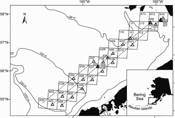
In this study, we report recent observations of polychaete assemblages in the south-eastern Bering Sea (Figure 1). This new data stemmed from an initiative to update information on the benthic community in the entire EBS to support habitat research. We used these new data to conduct an exploratory analysis of the correspondence between polychaete assemblages and environmental variables, particularly surficial sediment types that define the benthic habitat. We also assessed the co-correspondence (ter Braak & Schaffers, Reference ter Braak and Schaffers2004) between the distributions of the polychaete families and some known groundfish polychaete-feeders. For direct evidence of trophic interaction, we compared the polychaete prey composition in the stomach contents of selected groundfish with the observed polychaete assemblages. We then synthesized this information for insight into the habitat linkages between polychaete assemblages and groundfish predators, and the potential use of polychaete assemblages in defining habitat suitability for these groundfish in the EBS.
Eastern Bering Strait trawl cells traversed by survey tracklines (dashed lines). Grab sampling stations are indicated (triangles). Most grab stations are at trawl station locations at or near the centre of trawl cells.

MATERIALS AND METHODS
Sampling
An acoustic survey to characterize benthic habitats of the south-eastern Bering Sea seafloor was conducted on the NOAA ship ‘Fairweather’ during 6–20 August 2006. Sonar systems were used in surveying tracklines that totalled about 1295 km (Figure 1). The tracklines were laid along the depth gradient over a range of 20–160 m. The tracklines intersected 28 of the fixed EBS bottom-trawl-survey stations that are sampled annually by the Alaska Fisheries Science Center's (AFSC) Resource Assessment and Conservation Engineering (RACE) Division. Each fixed trawl station is located approximately at the centre of a 20 × 20 nautical mile grid cell (Figure 1). Standardized catches (kg ha−1) by species are calculated at each trawl station of the survey (Lauth & Acuna, Reference Lauth and Acuna2007).
During the acoustic survey, a sediment grab sample and an infauna grab sample were taken at 26 selected stations within 20 of the 28 trawl cells along the tracklines for biological and geological habitat information. These groundtruthing stations were selected to represent distinct seafloor characteristics—as interpreted from backscatter mosaic generated by a Klein 5410Footnote 1 sidescan sonar. A 0.1-m2 Van Veen grab mounted on a Seabed Observation and Sampling System (SEABOSS; US Geological Survey, 2000) was used to successively collect one infauna sample and one sediment sample at each groundtruth station. Positions of the stations were determined with an ultra-short baseline (USBL) system. The depth of penetration of the grab was the height of the intact sample in the grab measured down from the centre of the surface of the sample. For granulometry, a subsample of the sediment grab sample was taken for analysis using a Malvern Mastersizer 2000 laser particle sizer (McCave et al., Reference McCave, Bryant, Cook and Coughanowr1986), which can detect a minimum particle size of 2 × 10⁻⁵ mm.
For infauna, the entire grab sample was washed through 1 mm steel mesh screen and pre-sorted for benthic macroinvertebrates, which were fixed in 10% buffered formalin with rose Bengal stain for 2–3 days, then drained and preserved in 50% isopropyl alcohol. Later, in the laboratory, macroinvertebrates were sorted from the samples and identified to at least the family level. Family is considered a sufficiently high taxonomic resolution for polychaetes for use in many benthic ecology studies (Grebmeier et al., Reference Grebmeier, Feder and McRoy1989; Olsgard et al., Reference Olsgard, Brattegard and Holthe2003; Quijón & Snelgrove, Reference Quijón and Snelgrove2006; Włodarska-Kowalczuk & Kędra, Reference Włodarska-Kowalczuk and Kędra2007), and was the only practical taxonomic level for this study. Abundance a pq (individuals 0.1 m−2) and biomass b pq (g 0.1 m−2, alcohol-preserved blotted wet weight) were recorded for each family p in each sample q. Weight of an individual was not taken unless it was the only one of the family in the sample. Sample mean weight (w) of an individual of family p in sample q was calculated as: w = b pq/a pq. Overall mean weight (W) of an individual of family p was calculated over all samples as: W = B/A where B is total biomass of family p and A is total abundance of family p:  ;
 .
Community analysis
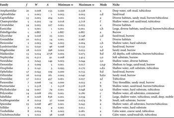
A total of 30 polychaete families were identified (Table 1). Shannon diversity (H′) and Richness (i.e. number of taxa) (S) (Legendre & Legendre, Reference Legendre and Legendre1998) were calculated for polychaetes at the family level for each station. H′ ranges from 0 (one taxon) to log S (all taxa equally dominant), with decreasing H′ with fewer dominant taxa. To reduce the influence of rare occurrences, only the 26 polychaete families that occurred at more than one grab station were used in community analyses.
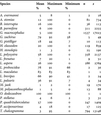
Frequency of occurrence (f) of polychaete families at 26 grab stations. Only the 26 families present at more than one station were included in analyses. Overall mean weight (W; in grams) and total number of individuals (A) over all samples, and minimum and maximum sample mean weight of an individual (w) are given (see Materials and Methods—Sampling for definition; where f = 1, i.e. only one sample where family was present, minimum w = maximum w). Each family is generally assigned to one or more feeding modes (a, surface deposit-feeder; b, subsurface deposit-feeder; c, carnivore; d, detritivore; f, filter-feeder; h, herbivore; o, omnivore; p, parasite; s, scavenger), and characteristics of commonly known habitat niches are noted (Fauchald & Jumars, Reference Fauchald and Jumars1979; Rouse & Pleijel, Reference Rouse and Pleijel2001). First three letters of the family are used as label in ordination diagrams.

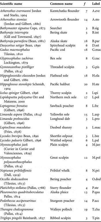
Spatial distributions of selected groundfish and epibenthic invertebrate species from the AFSC RACE bottom-trawl survey conducted in the period of May–August 2006 were compared with that of polychaete assemblages. All 28 selected species are groundfish except for one invertebrate (Table 2), and so hereafter for brevity are referred to collectively as the set of groundfish. These species were selected because: (1) they have diets that include polychaetes (Himmelman & Hamel, Reference Himmelman and Hamel1993; Yang, Reference Yang2003; M.-S. Yang, unpublished data); and (2) they occurred in more than one of the 20 trawl cells where grab samples were taken (Figure 1).
Frequency of occurrence (f) of groundfish taxa at the 20 trawl stations transected by the survey. Labels are used in ordination diagrams.

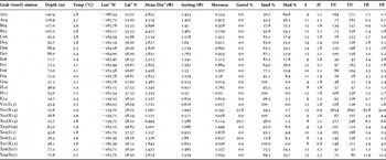
Grab samples were paired with trawl catches in analysis. Sixteen of the grab samples were taken at trawl stations and were paired directly (i.e. ‘matched’ Stations A–K; Figure 1). Ten were taken near trawl stations (i.e. ‘unmatched’ Stations V–X) and each was paired with trawl catches from the nearest trawl station. In some cases, several grab samples may be paired with the catches from the same trawl station—e.g. X01, X02, X03 were all matched with K14 (Table 3).
Grain-size parameters and the richness (S), diversity (H′), total number and biomass (g 0.1 m−2) of polychaetes at each grab station. Both the total number (TN) and biomass (TB) of only those polychaete families used in analysis (Table 1), and the total number (TN′) and biomass (TB′) of all polychaetes captured (including those of families not used in analysis and those unidentified) are given. Grab samples were paired with bottom-trawl samples for correspondence analysis. Stations A–K are ‘matched’—i.e. each station has both grab and trawl samples. An ‘unmatched’ grab station is paired with a nearest trawl station (in parentheses).

1longitude; 2latitude; 3diameter.
Separate canonical correspondence analyses (CCA) were conducted between matrices of environmental variables and polychaete families (biomass and abundance, respectively), and between matrices of environmental variables and groundfish species (standardized catch). Biotic data were 4th-root transformed to reduce the influence of highly dominant taxa and downweigh noise (Clarke & Warwick, Reference Clarke and Warwick2001). CCA is a constrained ordination technique commonly used in community analysis to unravel how a multitude of species simultaneously respond to environmental factors. CCA assumes that species response to environmental gradients is unimodal, which, from preliminary analyses, is more appropriate to the ecological data examined here than ordination techniques that assume a linear response. It selects axes that are linear combinations of environmental variables that best explains variations in a matrix of species abundance (ter Braak & Verdonschot, Reference ter Braak and Verdonschot1995). Community structure unrelated to the environmental variables is ignored.
Ten environmental variables were considered for CCA (Table 3) that directly or indirectly influence species distribution (Freeman & Rogers, Reference Freeman and Rogers2003; Valavanis et al., Reference Valavanis, Pierce, Zuur, Palialexis, Saveliev, Katara and Wang2008). Sediment properties are especially important in organizing benthic communities (Grebmeier et al., Reference Grebmeier, Feder and McRoy1989). Six sediment-related variables were derived from grab samples: mean percentage weights of gravel (grain-size diameter >2 mm, or <-1Φ), sand (0.0625–2 mm, or –1–4Φ), and mud (<0.0625 mm, or >4Φ); mean, sorting (standard deviation) and skewness (symmetry) of the grain-size distribution (Folk & Ward, Reference Folk and Ward1957). Four were non-sediment-related variables: latitude, longitude, water depth and bottom temperature. Temperature and depth directly affect the physiology of species; geographical coordinates are surrogates for many environmental gradients correlated with species patterns (Guisan & Zimmermann, Reference Guisan and Zimmermann2000), e.g. sea surface temperature and proximity to shore. Bottom temperature at or near each grab station was obtained from the 2006 EBS bottom-trawl survey. Each environmental variable was standardized (mean = 0, variance = 1) to enable comparable influence among variables with different measurement units (Griffith et al., Reference Griffith, Kaufmann, Herlihy and Hill2001). Hereafter, reference to gravel, sand, or mud as an environmental variable implies ‘mean percentage weight of’ that sediment type.
A subset of significant environmental variables was chosen by the stepwise forward selection procedure (ter Braak & Verdonschot, Reference ter Braak and Verdonschot1995; Legendre & Legendre, Reference Legendre and Legendre1998; Jaworski & Ragnarsson, Reference Jaworski and Ragnarsson2006) implemented in the R package ‘vegan’ (Oksanen, Reference Oksanen2004). Briefly, the procedure is as follows:
Let Y be the polychaete assemblage table and Xi be the i th standardized environmental variable.
(1) CCA of (Y, Xi) is conducted for each i as the only environmental variable. X1 is chosen that gives the highest significant eigenvalue (λ) for the CCA axis.
(2) CCA of (Y, X1 + Xi) is conducted, where i ≠ 1. X2 is chosen as the only additional environmental variable that gives the highest significant sum of eigenvalues in conjunction with X1.
(3) Repeat (2), adding on Xi until no other variable is significant.
Significance of the CCA axis (eigenvalue) is assessed based on a pseudo F-statistic (ratio of constrained and unconstrained total inertia) in an ANOVA-like permutation test (Y permuted by row, i.e. stations, at random) at α = 0.05, β = 0.01. The observed F is tested for significance against the distribution of F from 1000 permutations. An approximate Bonferroni correction α* = α/k, where k is the number of independent tests (= number of significant Xis), is applied to ensure that the overall significance level of the model is ≤ α for all k (Bland, Reference Bland2000).
The subset of significant environmental variables used in the CCA of polychaetes was then used in the CCA of groundfish, with the addition of two standardized descriptors of polychaete assemblages—total polychaete biomass and diversity (H′). These variables were used to test whether the polychaete assemblage itself or its significant driving factors also affect the ordination of groundfish. The significance of each descriptor (environmental subset and polychaete assemblage indices) was tested by random permutation of the groundfish community table by row as stated before. Since this subset of environmental variables for the CCA of groundfish was not chosen by stepwise forward selection as for the CCA of polychaetes, every order of entering these variables into the CCA was tested to assess the overall marginal significance of each one.
The CCA ordination diagram, or joint plot, summarizes visually the relationships among sites and species (ter Braak & Verdonschot, Reference ter Braak and Verdonschot1995; Legendre & Legendre, Reference Legendre and Legendre1998). Simply, in the joint plot, a species ordinated close to a site implies that it is more likely to be found there; sites that are close together in the joint plot have similar environmental characteristics and species composition. An environmental descriptor axis is displayed as an arrow radiating from the origin of the ordination. The magnitude of the environmental variable increases in the direction of the arrow. The ranking of sites (species) along an environmental gradient can be approximated by projecting them perpendicularly onto the arrow. The further the objects are from the origin, the more distinct the pattern, i.e. less widely distributed, associated with fewer sites. Here, sites scores have been standardized to unit variance so that in the plot their dispersion along each axis does not vary according to the relative importance of the axis.
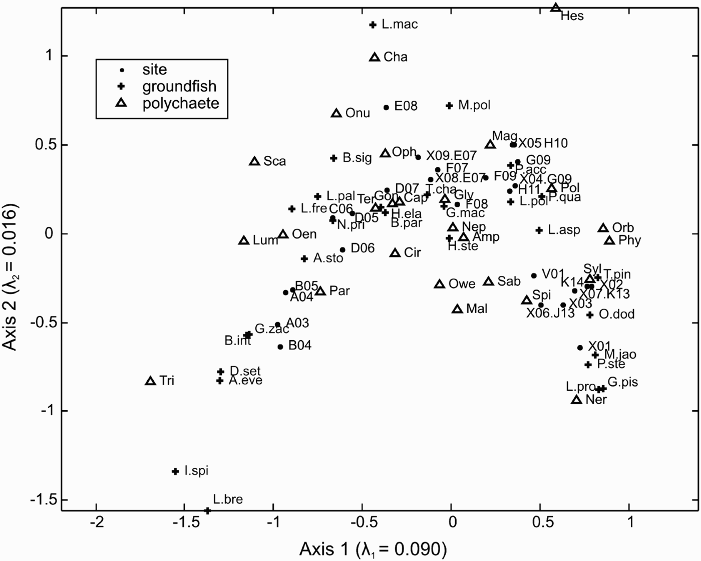
A descriptive, symmetrical co-correspondence analysis (CO-CA) (ter Braak & Schaffers, Reference ter Braak and Schaffers2004) was conducted to identify common distribution patterns between polychaete families and groundfish species. The measure of association is the covariance between the relative abundance or biomass of the two communities. This relatively new method integrates into one step the indirect, two-step approach of applying correspondence analysis to separate species data sets, and then correlating the resulting ordination axes. To relate the correspondence analyses of two communities in CO-CA, a set of common site weights (the site's total abundance of the species in the analysis) has to be applied to both community data tables (site × species). The common site weights were defined in this analysis as the average of the row sums (site weights) of each community data table as suggested in ter Braak & Schaffers (Reference ter Braak and Schaffers2004). The analysis was conducted in MATLAB® (2008a, The Mathworks, Inc., Natick, MA) using their codes (ter Braak & Schaffers, Reference ter Braak and Schaffers2004).
The symmetrical CO-CA joint plot displays the relative distributions of polychaete families and groundfish species at the sampling stations. The CCA ordinations of polychaete families and groundfish species were effectively joined together through applying multipliers to the species scores (coordinates) of each community to scale their ordination axes for optimal representation of the association between the two data sets in the plot (ter Braak & Schaffers, Reference ter Braak and Schaffers2004). The general interpretations are similar to the CCA joint plot.
Stomach content
Dietary information for the selected groundfish species from 1995–2007 was obtained from the AFSC Groundfish Food Habits database (Yang, Reference Yang2003). The taxonomic composition and percentage weight of polychaetes in the stomach contents of groundfish were analysed to verify the associations between polychaete and groundfish communities suggested by CO-CA. The sampling unit was a haul. The contents of a stomach were first blotted with a paper towel and the total wet weight was recorded to the nearest one-tenth of a gram. Each prey item was examined under the microscope and classified to the lowest practical taxonomic level. In most cases, that was the family level. For this study, identification to above the family level (e.g. suborder) only was considered unidentified. Weights of each prey taxon were recorded. The percentage weight of a prey taxon was averaged over all stomachs of a species collected in a haul.
RESULTS
Sediment
The depth of penetration of the Van Veen grab ranged from 6.8 to 16 cm on all the samples. It was ≥10 cm on all samples except for the three stations that contained gravel: X01 (6.8 cm), X03 (9.5 cm), and X08 (8 cm). Sediment grain-size trended from large to small towards the offshore (Table 3). Gravel was only notable in the inshore (depth <50 m) samples. Sand was generally dominant, except in the offshore (depth >100 m) samples, where it shifted to mud.
Fine-scale spatial variability in surficial sediment texture was most evident nearshore in the north-eastern part of the survey area. A cluster of grab stations (K14, X01, X02, X03, X06, X07 and V01) was located in close proximity in trawl cells K14 and J13 (Figure 1). However, the grain-size composition among these stations varied widely (Table 3). X01, X02 and X03 were at almost the same location, but X02 had no gravel component. Similarly, X06 and X07 had dissimilar grain-size compositions despite almost identical locations.
Polychaete infauna
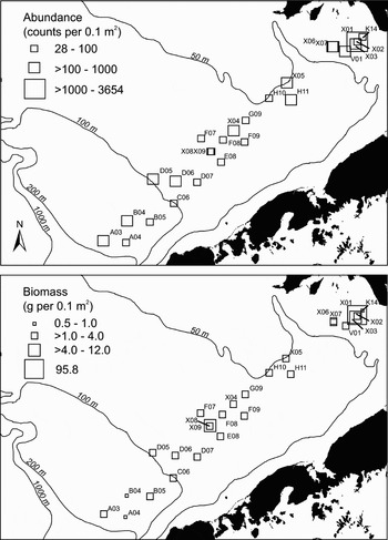
Richness ranged from 6–15 families at a station with an average of 11 ± 3 (SD) (Table 3). In general, relatively lower diversity and richness of families were found in shallow water. The highest abundance and biomass were nearshore at X01 (Table 3; Figure 2). The lowest abundance was mid-shelf at F09; the lowest biomass was found both inshore at K14 and offshore at A04. Considerable variability in abundance and biomass existed nearshore, as seen among stations X01, X02, X03 and K14 in the same trawl cell.

Abundance, weights and general notes on ecological niche are given in Table 1 for each of the 30 polychaete families identified. Maldanidae was the most abundant family in this study (A = 2758), with the greatest number occurring at X01 (Table 3). Discounting those families with only a single individual collected, Nephtyidae had the highest overall mean weight (W = 0.312 g), which was an order of magnitude greater than the overall mean weight of Maldanidae (W = 0.024 g). Abundant families tended to have a low overall mean weight of individuals. There was usually a wide variation in sample mean weight of individuals in a family (e.g. for Nephtyidae, w ranged from 0.008 to 3.415 g), suggesting that either there were multiple genera or species represented in the family, or that the weight of an individual of the same genus or species differed considerably among stations.
Distribution patterns were examined (not shown). Some families ranged widely over the study area, whereas others had more limited range. Among the latter, Chaetopteridae and Hesionidae generally occurred in depths within 50–100 m; Glyceridae in depths >100 m; Lumbrineridae, Oenonidae, Onuphidae, Scalibregmatidae, and Trichobranchidae were found offshore in depths >75 m; Magelonidae, Orbiniidae, Phyllodocidae, Polynoidae, and Syllidae were found inshore in depths <75 m.
Ordination
INFAUNA—ENVIRONMENT
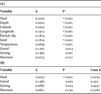
Abundance and biomass gave similar results in ordination analysis. Therefore, only results with respect to abundance are reported. In forward selection, when each environmental variable was tested alone (marginal effect), mud contributed the highest significant eigenvalue to the ordination of polychaetes (Table 4a). Thus, it was the first environmental variable selected. In subsequent searches, gravel and sorting, in order, were significant when other significant variables found in previous searches were already in the model (conditional effect). After applying the approximate Bonferroni correction, α* = 0.017, sorting was also eliminated (P > α*). Mud and gravel were thus the only two environmental variables used in subsequent ordination analysis.
Forward selection of environmental variables in canonical correspondence analysis (CCA) of polychaete assemblages—eigenvalue (λ) measures the fit of the model; P is the significance level of the additional CCA axis introduced by the selected variable: (A) each variable is the sole environmental variable in the model (marginal effect); (B) variables are listed in the order of entry in the model (conditional effect). For (B), each subsequent variable to enter is selected because it has the highest significant addition of λ to the model. Cumulative λ is the total eigenvalue of the model inclusive of the latest selected variable (may be slightly different from the sum of individual λ's, which is calculated exclusive of the latest selected variable).

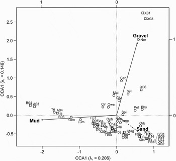
In CCA, axis 1 (λ1 = 0.2057) was closely correlated with the mud gradient and axis 2 (λ2 = 0.1462) with the gravel gradient (Figure 3). The two axes explained 25% of the total inertia (similar to variance) in the community data. Using a rule of thumb of a strong gradient being λ ≥ 0.30 (ter Braak & Verdonschot, Reference ter Braak and Verdonschot1995), these gradients were moderate in strength. Since the fractions of mud, gravel, and sand sum to unity, sand content was linearly dependent on mud and gravel content. A descriptor arrow for the sand gradient was approximated (of arbitrary length and extending from the origin between and away from the gravel and mud arrows) in the ordination plot to facilitate discussion (Figure 3).
Canonical correspondence analysis (CCA) of polychaete assemblages. The two CCA axes with the highest eigenvalues (λ) are displayed. Labels for stations (squares) and taxa (circles) were moved slightly in some cases to avoid overlap. Top and right axes (unlabelled) are scaled for environmental arrows. The arrow for sand is approximated (not to scale).

The ranking of stations and taxa along the sediment gradients was summarized in the CCA plot (Figure 3). Stations X01, X03 (each with ~50% gravel; Table 3), and X06 (20% gravel) were ordinated accordingly along the gravel gradient; likewise, B04 and A03 were appropriately ranked along the mud gradient (~70% mud). The cluster of stations that included G09, V01, X02, X07 and H11 at the far end of the approximated sand gradient all had 100% sand. In the CCA, the ordination of each polychaete family along the environmental arrows reflected its affinity for that environment. Families near the origin were usually not well-defined in terms of preference for the environmental variables considered. Many stations and families fell near the origin between the mud and sand environments (Figure 3). Those stations were characterized by mixed mud and sand, as were the majority of stations (Table 3), and many of those families are generally known as deposit-feeders, e.g. Ampharetidae and Capitellidae. The polychaete families most closely associated (in rank order) with muddy sediment were Trichobranchidae, Oenonidae and Lumbrineridae. Nereididae, Sabellidae, Syllidae, Maldanidae and Glyceridae were the families most closely associated with gravelly sediment. Hesionidae, Orbiinidae and Magelonidae were the families most closely associated with sandy sediment. Families at the extreme end of the environmental gradient were rare. It may truly indicate environment preference, or it may be just a chance occurrence. For example, the little known and rare Hesionidae (Fauchald & Jumars, Reference Fauchald and Jumars1979) was present only at two stations with 100% (G09) and 95% sand (X05) (Table 3) and was ordinated at the far end of the sand arrow (Figure 3).
GROUNDFISH—ENVIRONMENT
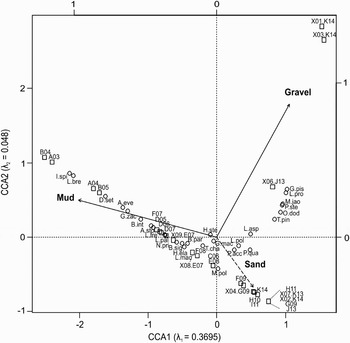
Mud, gravel, total polychaete biomass, and H′ were tested for significance in an initial CCA of groundfish species. Mud was the most significant factor, and total polychaete biomass the least, in the ordination of groundfish species. Gravel and diversity of the polychaete assemblage had approximately equal influence. Of the 24 possible combinations of ordering the four descriptors in entry to CCA, mud was significant (P < 0.001) in all combinations. Gravel was significant in 14 combinations (7 at P < 0.001; 4 at P < 0.01; 3 at P < 0.05), H′ was significant in 16 combinations (11 at P < 0.01, 5 at P < 0.05). Total biomass was significant (P < 0.01) only for the six combinations when it was the first variable to enter the analysis. In the CCA of groundfish species with only mud and gravel as environmental variables (Figure 4), the correlations between sediment gradients and CCA axes, and the ordination of stations relative to the gradients were similar to those in the CCA of polychaetes (Figure 3). For groundfish, axis 1 (λ1 = 0.3695) was closely correlated with the mud gradient and axis 2 (λ2 = 0.0480) with the gravel gradient. The two axes explained 48% of the total inertia in the community data.
Canonical correspondence analysis (CCA) of trawl species. The two CCA axes with the highest eigenvalues (λ) are displayed. Trawl station paired with an ‘unmatched’ grab station is prefixed with the label of the grab station (see Table 3 and Materials and Methods—Community analysis). See Figure 3 for other notations.

The variability in the distributions of most groundfish is more strongly related to the mud gradient than the gravel gradient in this analysis (Figure 4). Icelus spiniger Gilbert, 1896 and Lycodes brevipes Bean, 1890 were ordinated at the extreme far end of the mud gradient. They were rare in trawl samples, occurring respectively at only two and three stations (Table 2). Dasycottus setiger Bean, 1881 and Atheresthes evermanni Jordan & Starks, 1904 also ranked high along the mud gradient. They generally had higher biomass where the mud content was high. Myoxocephalus polyacanthocephalus (Pallas, 1814) was associated with sandier sediment. A cluster of species that included Gymnocanthus pistilliger (Pallas, 1814) and Limanda proboscidea (Gilbert, 1896) were associated with gravelly sediment. Pleuronectes quadrituberculatus and Lepidopsetta polyxystra were associated with the predominantly sandy sediments of inner (depth <50 m) and mid-shelf (50–100 m) stations (Table 3). However, species that appeared to be associated with sand or gravel were ordinated relatively near the origin of those gradients (Figure 4), which does not suggest a particularly strong association with those specific sediment types.
CO-CORRESPONDENCE BETWEEN POLYCHAETE ASSEMBLAGES AND GROUNDFISH SPECIES
Although the first two CO-CA axes explained 61% of the total inertia in the groundfish data and 38% of the polychaete data, overall correspondence between groundfish species and polychaete families was considered weak judging from eigenvalues (ter Braak & Verdonschot, Reference ter Braak and Verdonschot1995; λ1 = 0.090, λ2 = 0.016; Figure 5). Axis 1 was principally correlated with the environmental variable mud (Pearson r = –0.91), and secondarily with sand (r = 0.65) and gravel (r = 0.38). Axis 2 was principally correlated with sand (r = 0.53) and gravel (r = –0.45), and secondarily with mud (r = –0.26). In a trial analysis of the data sets using predictive CO-CA (groundfish as response, polychaetes as predictor), the first two axes were very similar to those from symmetrical CO-CA reported here. The two axes from predictive CO-CA predicted about 42% of the groundfish data, but a permutation test of the significance of the axes (ter Braak & Schaffers, Reference ter Braak and Schaffers2004) showed that only the first CO-CA axis was significant (P < 0.001), and the second and higher axes were not (P > 0.15).
Co-correspondence between polychaete assemblages and trawl species. The two canonical correspondence analysis axes with the highest eigenvalues (λ) are displayed. ‘Unmatched’ grab station is prefixed with the label of the nearest trawl station it is paired with (see Table 3 and Materials and Methods—Community analysis).
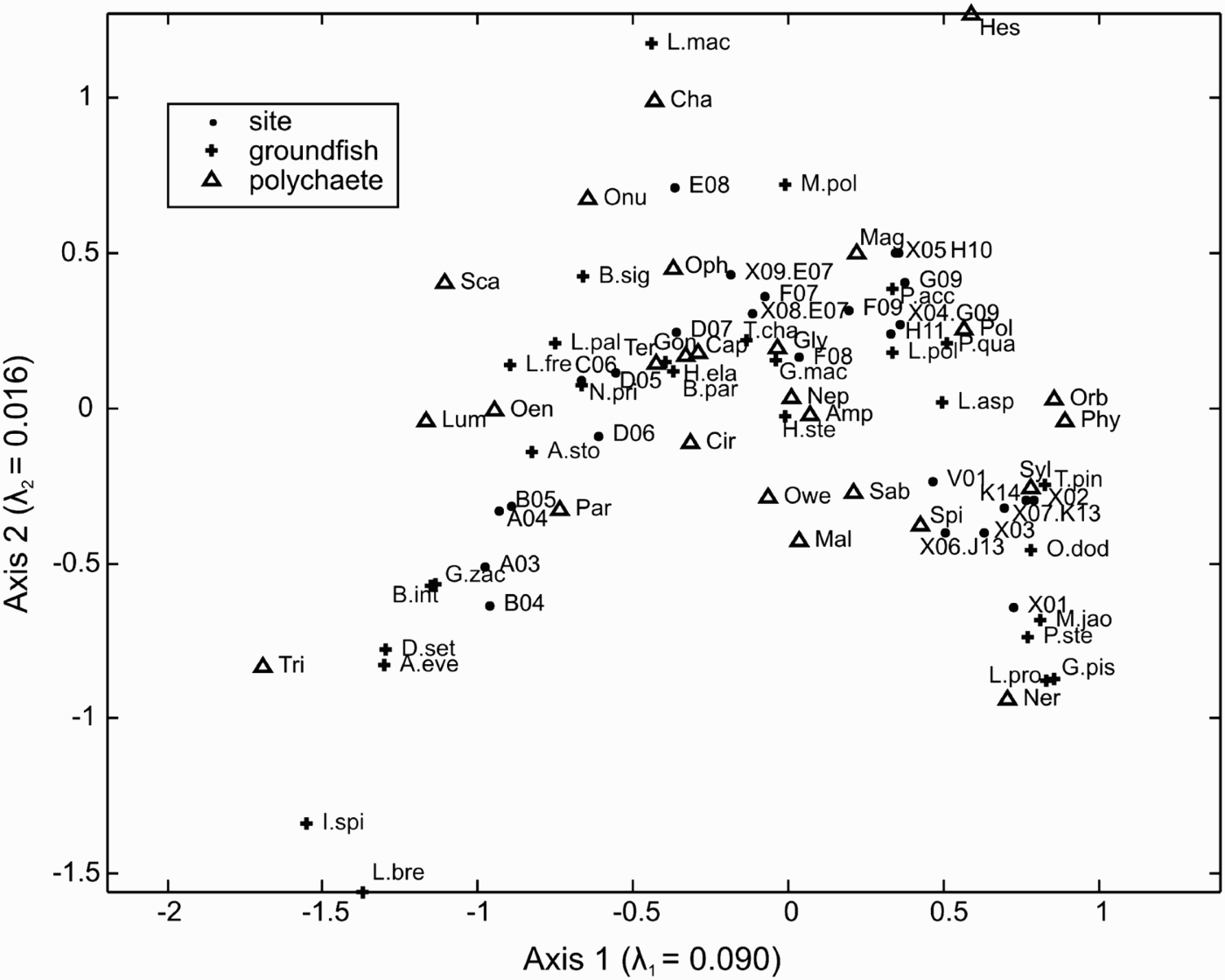
Groundfish and polychaetes in corresponding positions with respect to the origin are positively associated. We focus reporting on the stronger associations, i.e. species far from the origin. Dasycottus setiger and Atheresthes evermanni were close together in CO-CA as in CCA (Figure 4). Trichobranchidae was the polychaete family ordinated nearest these fish. The centre of mass of all three taxa were near the muddy Stations A–B offshore (≥ 100 m; Table 3, Figure 1). Leptoclinus maculatus (Fries, 1838) (frequency of occurrence = 3; Table 2), Lycodes brevipes (3), and Icelus spiniger (2) were rare and thus were ordinated at/near the boundaries of the plot; likewise the polychaetes Nereididae (2) and Hesionidae (2) (Table 1). Taxa near the origin, e.g. Nephtyidae and Ampharetidae, were generally widely distributed among stations (Table 1) and over different sediments. Hippoglossus stenolepis also exhibited a universal presence (Table 2) and biomass across all stations. Species along the positive axis 2 (e.g. Myoxocephalu polyacanthocephalus, Chaetopteridae and Onuphidae) were distributed in the mid-shelf area at Stations D–G, and were associated with sandy sediments (Figure 5).
STOMACH CONTENTS
Most polychaetes in stomach contents were unidentified. Those that were identified are of families found in the infauna samples of this study (Table 1), with the exception of Euphrosinidae, Sabellariidae, Sternaspidae and Tomopteridae. Sternaspidae has only one species, Sternaspis scutata Ranzani, 1817. Tomopteridae is a pelagic family (Fauchald & Jumars, Reference Fauchald and Jumars1979), and was found only in the stomachs of the demersal Gadus macrocephalus and Theragra chalcogramma (Table 6). Families found in the infauna samples, but not confirmed in the stomach records examined here, were Hesionidae, Megalonidae and Paraonidae. No stomach data are available in the database for Bathymaster signatus Cope, 1873, Triglops pingelii Reinhardt, 1837, Dasycottus setiger, Icelus spiniger and the whelk Neptunea pribiloffensis (Dall, 1919). The polychaetes in the relatively few stomach samples (Table 5) of Atheresthes evermanni, Leptagonus frenatus (Gilbert, 1896), Occella dodecaedron (Tilesius, 1813) and Platichthys stellatus (Pallas, 1788) were all unidentified (Table 6).
Polychaetes consumed as percentage of stomach weight of groundfish species for 1995–2007 (n, s = total number of hauls, stomachs sampled, respectively).

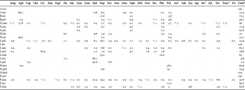
Percentage weight by family of total polychaetes found in stomachs of groundfish species between 1995 and 2007. Total number of hauls and stomachs in which polychaetes were present are given in Table 5. See Tables 1 and 2 for full names of polychaete families and groundfish species, respectively. Full names of the four polychaete families not in Table 1 (numbered) are given here.

1Euphrosinidae; 2 Sabellariidae; 3Sternaspidae; 4Tomopteridae; 5unidentified or identified to suborder only; Unid., unidentified
Most predators consumed a wide variety of polychaete taxa. For example, almost all polychaete families found generally in either infauna samples (Table 1) or stomach samples were found in the stomachs of Pleuronectes quadrituberculatus (Table 6). Although many families were consumed by P. quadrituberculatus, three were dominant by percentage of total polychaete weight: Nephtyidae (19.4%), Maldanidae (10.4%) and Terebellidae (6.6%). Ampharetidae was the most dominant family after these three (3.0%). All four families had relatively wide distributions over a mix of sediment types, as shown by their ordination near the origin in CCA (Figure 3).
Only Aphroditidae, Maldanidae, Nephtyidae, and Polynoidae comprised 10% of total polychaetes weight in the stomachs of more than one of the fish species examined. Aphroditidae, relatively large carnivores and one of the very few polychaetes caught in AFSC RACE bottom-trawl surveys, was the main polychaete family in the stomachs of larger fish such as Atheresthes stomias (66.1%, Table 6; number of hauls (n) = 81 and number of stomachs (s) = 734, Table 5), G. macrocephalus (17.6%; n = 1537, s = 17023), and Hippoglossus stenolepis (46.3%; n = 25, s = 190). Maldanidae comprised almost all the identified polychaetes in the stomachs of Lycodes brevipes (88.1%; n = 2, s = 24) and Lycodes palearis (95.6%; n = 4, s = 34). Other polychaetes that also occasionally comprised high percentages in stomach contents include: Terebellidae (P. quadrituberculatus—6.6%; n = 247, s = 1409), Phyllodocidae (Leptoclinus maculatus—10%; n = 1, s = 1), Opheliidae (Glyptocephalus zachirus—9.7%; n = 5, s = 49, Limanda proboscidea—9.1%; n = 2, s = 30) and Cirratulidae (L. proboscidea—62.9%; n = 2, s = 30). However, except for commercial fish species, the stomach sample sizes were very small.
Species that had exceptionally high polychaete consumption based on a relatively high number of samples were Lepidopsetta polyxystra (mean percentage of stomach weight = 58%, n = 358, s = 2137, Table 5), P. quadrituberculatus (57%, n = 247, s = 1409), Limanda aspera (26%, n = 286, s = 2769) and Hippoglossoides elassodon (20%, n = 119, s = 859). For L. polyxystra and P. quadrituberculatus, especially, high percentage consumption of polychaetes pervaded their entire depth-range of distribution in the EBS south of 60°N, where most samples were collected. Other species with a mean percentage of polychaetes in the stomach >10% include A. stomias, Bathyraja interrupta, G. zachirus, Gymnocanthus pistilliger, L. proboscidea, L. maculatus, L. brevipes, L. palearis and O. dodecaedron (Table 5). All these others but A. stomias and B. interrupta had relatively low number of samples (s < 100). Associations between predator and polychaete taxa suggested in CO-CA were not evident in the stomach data. For example, P. quadrituberculatus was not particularly close to any of its three principal prey families (Maldanidae, Nephtyidae and Terebellidae) in CO-CA (Figure 5).
DISCUSSION
Surficial sediment texture and composition are the most important environmental factors organizing polychaete assemblages in this study. This was also true historically for the benthic macrofauna community in the eastern Bering and Chukchi Seas (Stoker, Reference Stoker, Hood and Calder1981). The ordination of the families of polychaetes in relation to sediment gradients agrees generally with their functional ecology (Fauchald & Jumars, Reference Fauchald and Jumars1979; Table 1). Deposit-feeders (e.g. Ampharetidae and Capitellidae) are widely distributed in the sand/mud sediments that are ubiquitous in the study area. Burrowers (e.g. Trichobranchidae and Lumbrineridae) are associated with sediments with a high percentage of mud. Mobile, rapacious polychaetes (e.g. Nereididae and Syllidae) tend to be associated with harder substrates.
The dominant influence of sediment properties over species distribution has also been found in some groundfish (McConnaughey & Smith, Reference McConnaughey and Smith2000; Yeung & McConnaughey, Reference Yeung and McConnaughey2008). A large part of that influence probably stemmed from the important role sediment properties have in structuring the benthic community, which comprises the major prey groups for these fish. Sediment properties are surrogate for a suite of significant and interlinked hydrodynamic and ecological factors—e.g. primary productivity, currents/shear stress and detritus input (Stoker, Reference Stoker, Hood and Calder1981), which determine the quantity and quality of food available to the benthic community (Grebmeier et al., Reference Grebmeier, McRoy and Feder1988), and consequently to benthic-feeding fish.
We did not find any clear links between the spatial distributions of groundfish species and polychaete taxa at the family level. The stomach contents data set examined also did not indicate that predators select for specific polychaete families or guilds. Rather, most predators appear to be generalists. Usually, multiple polychaete families were found in a stomach, and often these families have wide geographical distribution. Pleuronectes quadrituberculatus and Lepidopsetta polyxystra were associated with sandy and muddy sediment types, an association that agrees generally with their known wide distribution (inshore to 100 m) in the EBS. Their principal polychaete prey according to their stomach contents, e.g. Maldanidae and Nephtyidae, are also widely distributed in those sediment types, which are prevalent on the EBS shelf. It appears that prey availability—a function of abundance, size, and catchability—could be the main driver of consumption.
Although the importance of polychaetes as a group to the diet of some benthic and demersal higher trophic level fauna has been clearly shown in the EBS and other oceans (e.g. Yang, Reference Yang2003; Quijón & Snelgrove, Reference Quijón and Snelgrove2005), interaction between specific polychaete taxa or guilds with predators is little known. In the Bay of Biscay (Serrano et al., Reference Serrano, Velasco and Olaso2003) identified dominant polychaete prey for some demersal and benthic fish as errant (mobile) carnivores, and hypothesized that the underlying factor for this apparent selectivity is availability. Errant carnivores are more active, hence susceptible to predation. This theory is supported in our study by the high percentage of the errant carnivore family Aphroditidae consumed by the larger fish species. Presence of these errant carnivores may also be enhanced in the study area because they benefit from organic matter generated by trawl disturbance and discards.
If the distribution and abundance of polychaete-feeders are mainly driven by prey availability, aggregate biomass of total polychaetes may be a sufficient if not better predictor of their distribution than taxonomically resolved polychaete biomass. For example, polychaete density was a major determinant of the quality of juvenile sole (Solea senegalensis) nursery habitat in the Tagus estuary, Portugal (Vinagre et al., Reference Vinagre, Fonseca, Cabral and Costa2006). However, in our observations, biomass of total polychaetes is of relatively low significance, compared to sediment variables, in predicting the distribution of predators. Other determinants of habitat quality may supersede the importance of food availability to predator distribution, e.g. shelter and camouflage may be better provided by sandy and muddy sediments for flatfish (Amezcua et al., Reference Amezcua, Nash and Veale2003). Further investigations with appropriate sampling designs will be necessary to resolve these questions.
Biases in the benthic, stomach, and trawl data used here could confound the resultant picture of the correspondence between prey and predators. Possible biases in benthic sampling, such as selectivity of sampling equipment and appropriate replication, are well documented (Ellis et al., Reference Ellis, Norkko and Thrush2000; Underwood & Chapman, Reference Underwood, Chapman, Eleftheriou and McIntyre2005). Compounded with unknown patchiness of the communities, these biases could lead to inaccurate description of community structure and estimation of biomass. Biases are also inherent in the stomach data. Most stomach samples examined in this study had a large fraction of unidentifiable polychaetes, so true absence of a polychaete taxon as prey cannot be established. Identification of polychaetes from stomachs is difficult mainly because of decomposition and fragmentation. It may be relatively easier for larger and more abundant polychaetes. In this study, Maldanidae is over 100 times more abundant than Nephtyidae in infauna samples, while mean individual weight of Nephtyidae is over 10 times greater than Maldanidae. Both families are dominant in stomach contents, but other families which are also abundant in infauna samples, e.g. Oweniidae, are relatively insignificant in stomach contents.
Groundfish distribution and associated stomach content data are obtained from summer bottom trawl samples, and may be biased towards adult sizes, target species, soft bottoms, and other ecological characteristics of the fixed study area. Therefore, this data set may not be able to resolve possible variations in polychaete consumption within species due to size/age, season, geographical location (Mahon & Neilson, Reference Mahon and Neilson1987; Tokranov, Reference Tokranov1990; Amezcua et al., Reference Amezcua, Nash and Veale2003), and habitat complexity (Gambi et al., Reference Gambi, Castelli and Guizzardi1997), etc that can confound ecological patterns. For example, Atheresthes stomias and A. evermanni are mainly piscivores, feed up in the water column, and have similar diets (Yang & Livingston, Reference Yang and Livingston1986). However, their association with polychaetes and mud may be stronger in the study area where they tend to be of a smaller size (M.-S. Yang, unpublished data). Also, this analysis indicates possible close association between species of ecological but not commercial importance, such as sculpins and skates, with polychaetes. However, diet data on these species are particularly scarce, so verification of trophic interaction is difficult.
Canonical correspondence analysis is a robust multivariate method widely used in community ecology and species-environment analysis (Legendre & Legendre, Reference Legendre and Legendre1998); CO-CA is a relatively new variation on that method (ter Braak & Schaffers, Reference ter Braak and Schaffers2004). CCA is robust to violations of the assumptions of normality and unimodality (ter Braak & Verdonschot, Reference ter Braak and Verdonschot1995), but does have some limitations that are widely documented (McCune, Reference McCune1997; Legendre & Legendre, Reference Legendre and Legendre1998; Millar et al., Reference Millar, Anderson and Zunun2005). One that may be especially relevant here is that it is less sensitive if family contains species with different environmental niches/optima (Griffith et al., Reference Griffith, Kaufmann, Herlihy and Hill2001). The niches of polychaete families given here are generalizations—within a family, sizes and diets (and thus sediment environment) of different species may vary widely (McHugh & Fong, Reference McHugh and Fong2002). Thus, further studies using polychaete species may yet reveal significant predator–prey linkages that are obscured by aggregation to the family level.
Coyle et al. (Reference Coyle, Konar, Blanchard, Highsmith, Carroll, Carroll, Denisenko and Sirenko2007) re-analysed the two historical benthic fauna data sets from the 1950s (Neyman, Reference Neyman and Moiseev1963) and 1970s (Haflinger, Reference Haflinger, Hood and Calder1981; Stoker, Reference Stoker, Hood and Calder1981) to relate changes in infauna biomass to climate effects. They found a significant increase in overall mean infauna biomass, including that of polychaetes, in the 1970s, which they attributed to increased benthic productivity resulting from the cooling of bottom temperature. They acknowledged the difficulties of comparing infauna studies with different sampling protocols, objectives and taxonomic expertise, in addition to patchiness of the communities. To minimize potential biases, the data were compared at the family taxonomic level.
Neither of the previous studies attempted to relate infauna assemblages to predator distributions, as we did. Also, our study area was limited to the south-eastern Bering Sea, where benthic biomass is expected to be lower relative to the north because of lower benthic productivity and higher predation pressure (Neyman, Reference Neyman and Moiseev1963; Haflinger, Reference Haflinger, Hood and Calder1981). Therefore, direct comparison of the presence and absence of particular polychaete taxa with previous studies may be not meaningful because of potential biases (Coyle et al., Reference Coyle, Konar, Blanchard, Highsmith, Carroll, Carroll, Denisenko and Sirenko2007), but generally the same families of polychaetes were common to all the studies. Haflinger (Reference Haflinger, Hood and Calder1981) clustered infauna into spatial groups, but concluded that the stability of groupings and distributions were uncertain. Long-term monitoring is necessary to evaluate patterns and trends in the community, and infauna studies like this one will contribute to building the database.
Given the limitations of the data sets used here (e.g. geographical range, environmental range, taxonomic resolution of polychaetes, sample size and size-range of predators), the present results are not definitive. The hypothesis that polychaete assemblages contribute to the distribution of groundfish predators should be re-examined with data that mitigate some of these limitations. The study methods and analytical approach used here nonetheless provide a strong basis for integrating future data sets to improve our understanding of the relationships between groundfish and their habitats. Future plans are to expand these investigations to the entire EBS. Incorporation of greater quantities of suitable data will help bring community patterns, species associations, and trophic interactions into clearer focus, and advance the ecological knowledge necessary to improve habitat descriptions and ecosystem understanding.
ACKNOWLEDGEMENTS
We thank R. Hibpschman and A. Whitehouse for identifying the polychaetes; G. Lang for querying the Food Habits Database; K. Smith for technical expertise on the SEABOSS and field sampling; and the officers and crew of the NOAA ship ‘Fairweather’ for their support in conducting the survey.