2 Model description

In this study, we use a two-layer QG model on the $\unicode[STIX]{x1D6FD}$ -plane in the presence of bottom topography where the topographic height increases linearly in the zonal direction (see figure 1 in Khatri & Berloff Reference Khatri and Berloff2018a ). The model is forced with a horizontally uniform, eastward background flow in the upper layer. The governing equations are (Vallis Reference Vallis2017)

(2.1) $$\begin{eqnarray}\displaystyle {\displaystyle \frac{\unicode[STIX]{x2202}\unicode[STIX]{x1D6F1}_{i}}{\unicode[STIX]{x2202}t}}+J(\unicode[STIX]{x1D713}_{i}-\unicode[STIX]{x1D6FF}_{i1}U_{b}y,\unicode[STIX]{x1D6F1}_{i})=\unicode[STIX]{x1D708}\unicode[STIX]{x1D6FB}^{4}\unicode[STIX]{x1D713}_{i}-\unicode[STIX]{x1D6FF}_{i2}\unicode[STIX]{x1D6FE}\unicode[STIX]{x1D6FB}^{2}\unicode[STIX]{x1D713}_{i}, & & \displaystyle\end{eqnarray}$$

where $J(a,b)$ is the Jacobian; $\unicode[STIX]{x1D713}_{i}$ and $U_{b}$ are the layer-wise velocity streamfunction and background flow, respectively. Index $i=1$ ( $i=2$ ) is for the top (bottom) layer and $\unicode[STIX]{x1D6FF}_{ij}$ is the Kronecker delta; $\unicode[STIX]{x1D708}$ and $\unicode[STIX]{x1D6FE}$ are eddy viscosity and bottom friction parameters, respectively, and $\unicode[STIX]{x1D6F1}_{i}$ represents the total PV in the layer, which is given as

(2.2) $$\begin{eqnarray}\displaystyle \unicode[STIX]{x1D6F1}_{i}=\unicode[STIX]{x1D6FB}^{2}\unicode[STIX]{x1D713}_{i}+\unicode[STIX]{x1D716}_{i}S_{i}(\unicode[STIX]{x1D713}_{2}-\unicode[STIX]{x1D713}_{1})+(\unicode[STIX]{x1D6FD}+\unicode[STIX]{x1D716}_{i}S_{i}U_{b})y+\unicode[STIX]{x1D6FF}_{i2}{\displaystyle \frac{f_{o}}{H_{2}}}\unicode[STIX]{x1D702}_{T}. & & \displaystyle\end{eqnarray}$$

Here, $\unicode[STIX]{x1D716}_{1}=-\unicode[STIX]{x1D716}_{2}=1$ and $S_{i}=f_{o}^{2}/g^{\prime }H_{i}$ ( $g^{\prime }=g(\unicode[STIX]{x1D70C}_{2}-\unicode[STIX]{x1D70C}_{1})/\unicode[STIX]{x1D70C}_{1}$ is the reduced gravity, where $\unicode[STIX]{x1D70C}_{i}$ is the layer density) is the stratification parameter; $\unicode[STIX]{x1D6FD}$ represents the meridional gradient in the Coriolis parameter and $f_{o}$ is the Coriolis parameter at some reference latitude. The last term on the right-hand side in (2.2) contains the contribution from topography. Here, $H_{i}$ is the layer thickness and $\unicode[STIX]{x1D702}_{T}$ is the topographic height. Since we consider a constant topographic slope in this study, we use notation $\unicode[STIX]{x1D6FD}_{T}=(f_{o}/H_{2})(\unicode[STIX]{x2202}\unicode[STIX]{x1D702}_{T}/\unicode[STIX]{x2202}x)$ in the rest of the paper.

Table 1.

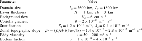
Parameter values used in the numerical simulations.

Following Khatri & Berloff (Reference Khatri and Berloff2018a ), we concentrate only on the effects of a zonally sloped topography. The magnitude of the zonal slope is chosen in such a way that $\unicode[STIX]{x1D6FD}$ always dominates over the topographic gradient term $\unicode[STIX]{x1D6FD}_{T}$ (see table 1). Thus, the baroclinic growth rates are not modified significantly in the presence of the sloping topography (see Chen & Kamenkovich Reference Chen and Kamenkovich2013, for details). Also, the change in depth is small compared to the thickness of the lower layer (for the largest slope magnitude, the change in depth is approximately 400 m). We could also study the effects of a meridional slope; however, for very mild meridional slopes, a meridionally varying topography is equivalent to an additional $\unicode[STIX]{x1D6FD}$ -effect in the bottom layer (from (2.1)), which has a negligible effect on the jet dynamics. In many places in the oceans, e.g. in the Southern Ocean, jets experience steep topography, where topographic gradients are much larger than the ones considered in this study. The results of this work are not directly applicable in those situations. This work would be more helpful in understanding the jet dynamics in regions away from continental boundaries where the topographic height changes moderately in space. However, the impacts of topography are also amplified in the two-layer QG model as the whole lower layer, which is 3 km deep in our case, experiences the effects of topography. We expect that, in real oceans, steeper slopes would be required to result in similar jet tilt angles and drift speed magnitudes which we observe in our simulations. The aim of this study is to analyse the sensitivity and stability of the tilted jets, robustly present in the equilibrated states of the considered flow regimes, as a function of the magnitudes of eddy viscosity and bottom friction parameters. So, we ran the simulations for a range of values of these parameters.

We considered a rectangular domain having $1024\times 512$ grid points and a grid resolution of 3.5 km. In this study, we mainly use doubly periodic simulations; nevertheless, the results are also compared with a channel simulation, in which we used partial-slip boundary conditions on the meridional sides. The second-order finite-difference method was used to discretise the equation (2.1) and the system was solved with an advanced flux preserving numerical scheme (Karabasov, Berloff & Goloviznin Reference Karabasov, Berloff and Goloviznin2009). The values used in the simulations are given in table 1. 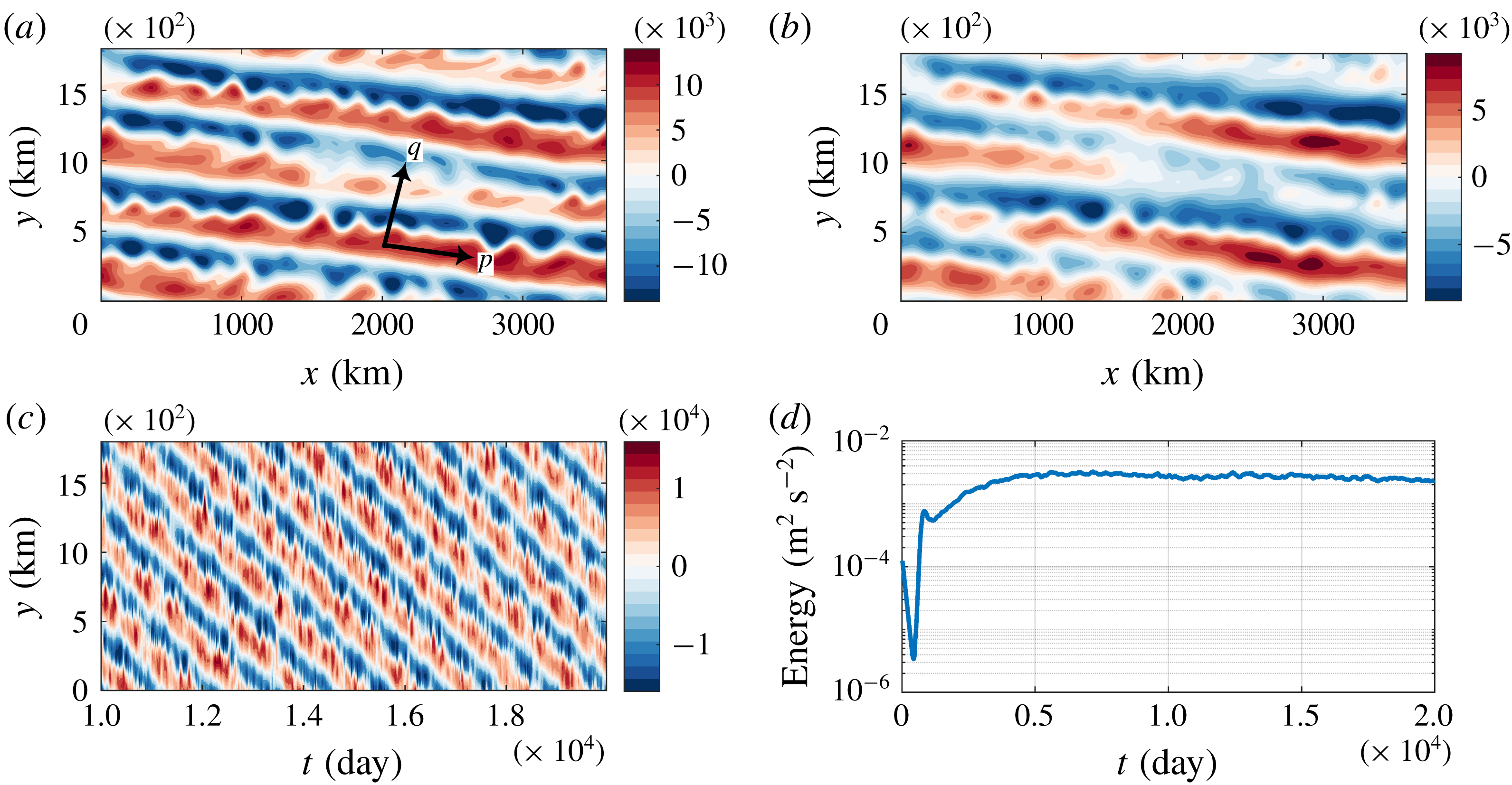Parameter $\unicode[STIX]{x1D6FD}$ and stratification parameters correspond to $30^{\circ }$ latitude and baroclinic Rossby radius of 25 km, respectively. The simulations were initialised from a perturbed state and, for the choice of parameters, the numerical runs converged quite quickly to statistical equilibrium. The total energy ( $1/(2A(H_{1}+H_{2}))\int _{A}[H_{1}|\unicode[STIX]{x1D735}\unicode[STIX]{x1D713}_{1}|^{2}+H_{2}|\unicode[STIX]{x1D735}\unicode[STIX]{x1D713}_{2}|^{2}+H_{1}S_{1}(\unicode[STIX]{x1D713}_{1}-\unicode[STIX]{x1D713}_{2})^{2}]\,\text{d}A$ , where $A$ is the area of the domain) time series (figure 1 d) shows that the system reached a statistically steady state by 5000 days. Further details of the simulations and spin-up can be found in Khatri & Berloff (Reference Khatri and Berloff2018a ). We ran the simulations for 20 000 days and used the data of the last 10 000 days for the analysis.

Figure 1.

(a,b) Snapshots of the streamfunction field in the top and bottom layers; (c) Hovmöller diagram of streamfunction field in the top layer ( $\unicode[STIX]{x1D713}_{1}$ along cross-section at the centre of the domain is plotted against time); (d) total energy (spatial mean) time series. $\unicode[STIX]{x1D6FD}_{T}=1.4\times 10^{-12}~\text{m}^{-1}~\text{s}^{-1}$ , $\unicode[STIX]{x1D708}=100~\text{m}^{2}~\text{s}^{-1}$ and $\unicode[STIX]{x1D6FE}=2\times 10^{-8}~\text{s}^{-1}$ were used in the simulation. The rest of the parameters were the same as in table 1.

In agreement with previous studies (Boland et al. Reference Boland, Thompson, Shuckburgh and Haynes2012; Khatri & Berloff Reference Khatri and Berloff2018a ), the jets tilt from the zonal direction and drift meridionally because of the zonally sloped topography (see snapshots of the streamfunction field, $\unicode[STIX]{x1D713}_{i}$ , in the top panels in figure 1). The mean barotropic PV isolines are tilted due to the presence of the sloped topography, and the jets tend to align with the mean barotropic PV isolines (see details in Boland et al. Reference Boland, Thompson, Shuckburgh and Haynes2012). In fact, PV gradients in the upper and lower layers have different orientations. The top layer experiences a background PV gradient only in the meridional direction, whereas, in the bottom layer, the background PV gradients have both zonal and meridional components (see (2.2)). The jets tilt in response to the titled mean barotropic PV isolines and drift meridionally to compensate for the PV advection due to the mean jets across PV isolines (Khatri & Berloff Reference Khatri and Berloff2018a ).

In the statistical equilibrium, the jets gain energy directly from the imposed background flow and lose energy to eddies. The direct transfer of energy from the background flow to the jets is possible through coupling between the jets and background vertical shear in the presence of topography (see Khatri & Berloff (Reference Khatri and Berloff2018a ) for details). However, this result is limited to continuously forced–dissipative systems, as Khatri & Berloff (Reference Khatri and Berloff2018a ) did not investigate the impacts of dissipation strength on the dynamics or explore the dynamics in the case of freely evolving turbulence over a sloped topography. In their study, both the tilted jets and eddies receive energy directly from the imposed vertical shear and, in the equilibrium state, this energy gain is balanced by viscous dissipation and bottom friction. It is not completely clear how the system would behave if the dissipation strength were reduced while maintaining the imposed background shear. In this paper, we explore the dynamics in weak-dissipation regimes. We study the jet dynamics in a number of simulations run with different magnitudes of eddy viscosity and bottom friction parameters. We observe that, in addition to the tilted jets, the system consists of many large-scale modes. We analyse these large-scale modes using EOF analysis, which is discussed in the next section.

3 EOF analysis

We employ EOF analysis technique to extract the dominant statistical modes from the solution field so that the streamfunction anomaly field is decomposed into a ranked set of mutually orthogonal spatial patterns and their principal components (see Hannachi, Jolliffe & Stephenson Reference Hannachi, Jolliffe and Stephenson2007, for a brief review). In order to compute EOFs, we used the streamfunction field in both layers together and, as a result, we obtained EOFs having the full three-dimensional structure, i.e. variation in the zonal and meridional directions as well as in the individual layers. For the purpose of comparison, we also computed EOFs separately in the upper and lower layers by applying the EOF analysis to the streamfunction field in the individual layers. The results were not significantly different. In both approaches, the leading EOFs were the same, although variances captured by different EOFs varied a little. 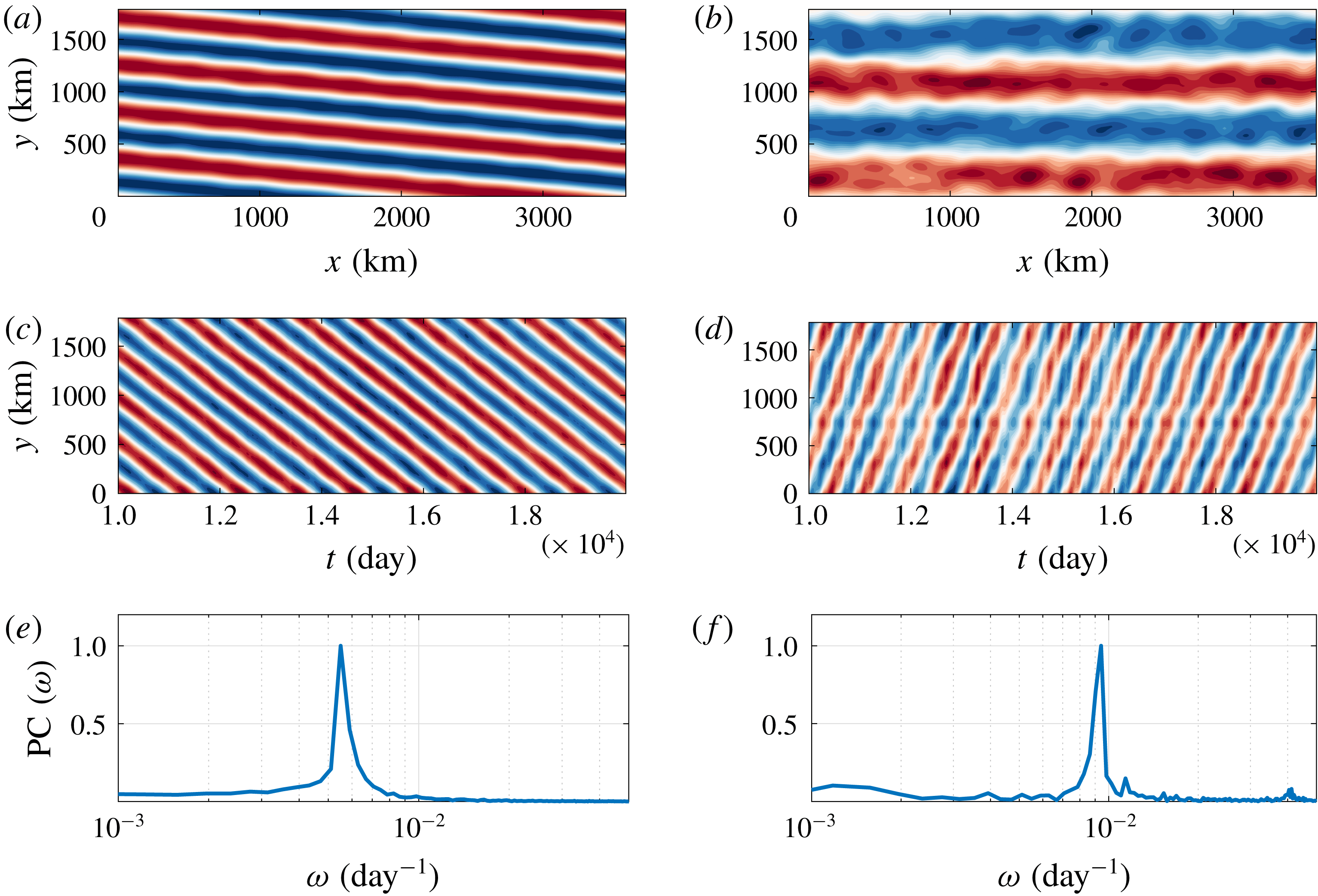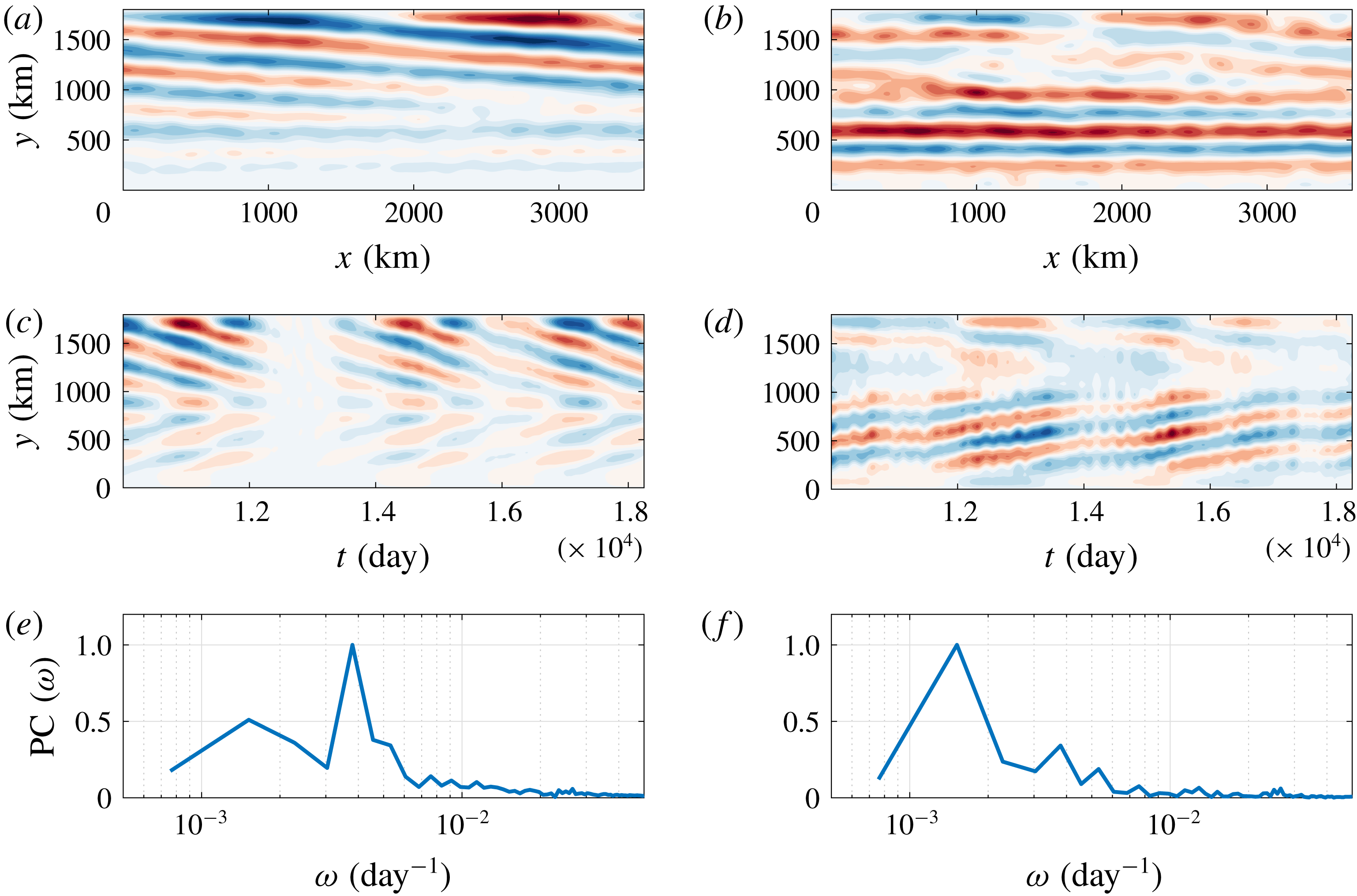For example, in the case of $\unicode[STIX]{x1D6FD}_{T}=1.4\times 10^{-12}~\text{m}^{-1}~\text{s}^{-1}$ , the first two EOFs together captured a variance of approximately 66 % when we computed EOFs in both layers together. On the other hand, when we used EOF analysis separately in the top and bottom layers, the variances captured by the first two EOFs were approximately 70 % and 60 % in the top and bottom layers, respectively. The leading EOFs are shown in figure 2, and it is intriguing that the following two types of large-scale patterns are captured by them. The first pair of EOFs, which are in quadratures, captures the titled jets (to be referred as $J$ mode, from here onwards), and the second pair of EOFs captures a purely zonal mode (to be referred as $Z$ mode, from here onwards). We multiplied the first and second EOFs to their principal components (PC) and added them to reconstruct the $J$ mode as a function of time. Similarly, we used the second pair of EOFs and the corresponding PC to reconstruct the $Z$ mode. We observed that both the $J$ and $Z$ modes propagate with constant speeds corresponding to distinct peaks in frequency as shown by the power spectra of PCs (see figure 2 e,f). The $Z$ mode propagates northward, i.e. opposite to the $J$ mode (see figure 2 c,d). We also verified the presence of the $J$ and $Z$ modes in a channel simulation (see appendix A). However, for simplicity, we only use doubly periodic runs in the rest of the paper.

Figure 2.

Leading EOFs of the streamfunction field in the simulation run in a doubly periodic domain (data interval was 10 000 days, i.e. 500 snapshots, for the EOF analysis) (a,c,e) EOF1-2 (b,d,f) EOF3-4. (a,b) Show the spatial structure of the EOFs in the top layer, and (c,d) show the Hovmöller diagram of the $J$ and $Z$ modes reconstructed using EOFs and their PCs (the modes along a meridional cross-section at the centre of the domain are plotted against time). Colour bar range is [ $-1,1$ ], blue to red. (e,f) Represent the spectra of PCs (normalised to unity) corresponding to the EOFs. The second and fourth EOFs are counterparts of the first and third EOFs, with the same spatial structure but shifted by $1/4$ of the time period. Only one of the EOFs is shown as both EOFs in a pair capture approximately equal variances. The $J$ and $Z$ modes together capture approximately 75 % of the variance. $\unicode[STIX]{x1D6FD}_{T}=1.4\times 10^{-12}~\text{m}^{-1}~\text{s}^{-1}$ , $\unicode[STIX]{x1D708}=100~\text{m}^{2}~\text{s}^{-1}$ and $\unicode[STIX]{x1D6FE}=2\times 10^{-8}~\text{s}^{-1}$ were used in the simulation. The rest of the parameters were the same as in table 1.

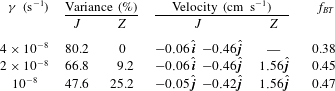
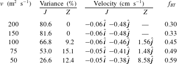
We further observed that the relative contributions of the $J$ and $Z$ modes are highly dependent on the magnitude of the slope, e.g. variances of the $J$ and $Z$ modes are listed in table 2. The contribution of the $J$ mode decreases with increasing the magnitude of the zonal slope while the contribution of the $Z$ mode increases. In fact, in the case of $\unicode[STIX]{x1D6FD}_{T}=2.8\times 10^{-12}~\text{m}^{-1}~\text{s}^{-1}$ , the $Z$ mode dominates the flow field. Together, the $J$ and $Z$ modes capture a majority of the variance in all simulations. The propagation (drift) velocities of these modes (table 2) were computed using the following relation:

(3.1) $$\begin{eqnarray}\displaystyle \boldsymbol{c}_{j}={\displaystyle \frac{\unicode[STIX]{x1D714}_{j}}{|\boldsymbol{k}_{j}|^{2}}}\boldsymbol{k}_{j}, & & \displaystyle\end{eqnarray}$$

where $\boldsymbol{c}_{j}$ is the propagation velocity, i.e. fundamental phase velocity, and $j$ stands for the mode; $\boldsymbol{k}_{j}$ and $\unicode[STIX]{x1D714}_{j}$ are the wavevector and peak frequency (in PC spectra), respectively, corresponding to the modes.

Table 2.

Variances and propagation velocities of the $J$ and $Z$ modes for different magnitudes of the zonal slope. Other parameters in the simulations were the same as in the caption of figure 2. Propagation velocity estimates obtained from numerical simulations (NS) and the linear dispersion relation (DR) are shown. $\hat{\boldsymbol{i}}$ and $\hat{\boldsymbol{j}}$ represent the zonal and meridional unit vectors, respectively. Here $n_{y}$ represents the number of meridional waves that is equal to the meridional width of the domain for the modes. In all three simulations, the zonal wavelength of the $J$ modes is equal to the zonal extent of the domain; $f_{BT}=\overline{E}_{BT}/(\overline{E}_{BT}+\overline{E}_{BC})$ represents the fraction of the mean barotropic KE, where $E_{BT}=1/2\int _{A}|\boldsymbol{u}_{BT}|^{2}$ and $E_{BC}=1/2\int _{A}|\boldsymbol{u}_{BC}|^{2}$ are the spatially integrated barotropic and baroclinic KE, respectively.

Khatri & Berloff (Reference Khatri and Berloff2018a ) found that drift speeds of the titled jets are in agreement with the phase speeds of linear Rossby waves, as estimated from the linear dispersion relation. Here, we compare the propagation speeds of both the $J$ and $Z$ modes with the estimates from the linear dispersion relation (see appendix B for details). The fundamental phase velocities computed using the dispersion relation are quite close to the actual propagation velocities of the $J$ and $Z$ modes in the numerical simulations. Over topographic slopes, jets drift to compensate for PV advection by the mean flow across PV isolines (Boland et al. Reference Boland, Thompson, Shuckburgh and Haynes2012; Khatri & Berloff Reference Khatri and Berloff2018a ). The $J$ mode advects PV across PV isolines in both layers, as the $J$ mode tends to be aligned with the mean barotropic PV isolines. On the other hand, the purely zonal $Z$ mode advects PV across PV isolines in the lower layer only. We hypothesise that the propagation of the $J$ and $Z$ modes in the opposite directions is due to PV advection by these modes in the opposite directions across PV isolines. For example, if the $J$ mode transports PV from the high PV to the low PV region, then the $Z$ mode transports PV from the low PV to the high PV region. As a result, the modes drift in the opposite directions. It is important to mention here that the $J$ and $Z$ modes only represent the leading tilted and purely zonal patterns observed in the EOF analysis. The meridional wavelengths of these modes are different in different simulations (see table 2), which is one of the reasons for the differences in drift speeds, i.e. modes with longer meridional wavelengths move faster. We also computed the ratio of the mean kinetic energy (KE) of the barotropic velocity component, $\boldsymbol{u}_{BT}=(H_{1}\boldsymbol{u}_{1}+H_{2}\boldsymbol{u}_{2})/(H_{1}+H_{2})$ , to the sum of the mean KE of the barotropic and baroclinic velocity, $\boldsymbol{u}_{BC}=\boldsymbol{u}_{1}-\boldsymbol{u}_{2}$ , components in the full flow field. We found that the flow field tends to be more barotropic due to the presence of the $Z$ mode as this energy fraction increases with an increase in the variance of the $Z$ mode. It is possible that the barotropic component of the flow field becomes stronger to dissipate more energy through bottom friction and stabilise the system, as the energy of the system increases with increasing the zonal slope magnitude (Khatri & Berloff Reference Khatri and Berloff2018a ). We discuss this aspect later in the paper.

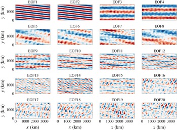
Apart from the $J$ and $Z$ modes, the higher EOFs capture many large-scale modes (first twenty EOFs are shown in figure 9), which have different tilt angles and spatial structures. Many of these EOFs are comparable to the $J$ and $Z$ modes in size and are also much larger than the size of mesoscale eddies. It is expected that these large-scale EOFs tend to align with PV fields in one of the layers or a linear combination of those PV fields; however, the tilt angles of the EOFs are greatly affected due to the imposed periodic boundary conditions in the simulations. All these EOFs, which capture different large-scale modes, can be broadly categorised into two families: the first family contains tilted EOFs ( $J$ family) and the second family contains purely zonal EOFs ( $Z$ family). The main purpose of this work is to understand why both tilted and zonal large-scale modes, irrespective of what their meridional width and drift speeds are, coexist. There is little use of studying individual EOFs, as they need not be unique in different scenarios, and relative contributions of EOFs can be different in different simulations.

The presence of various large-scale modes is in contrast to the case of zonal jets formed over a flat bottom, where the large-scale flow mainly consists of zonal jets. However, in the presence of a zonally sloped topography, the flow field tends to be a lot more complex. Although we mainly focus on the leading EOFs that capture two different types of modes, i.e. $J$ and $Z$ modes, many significant large-scale patterns emerge in higher EOFs (see appendix C). This suggests that the upscale transfer of energy from mesoscale eddies need not lead to the formation of only one type of alternating jets, rather many alternating patterns can coexist. Although most of the previous studies have focused on stationary zonal jets (Panetta Reference Panetta1993; Vallis & Maltrud Reference Vallis and Maltrud1993; Lee Reference Lee1997; Berloff Reference Berloff2005; Thompson & Young Reference Thompson and Young2007; Srinivasan & Young Reference Srinivasan and Young2012, and others), a few have studied the spatial and temporal variability in jets (Thompson Reference Thompson2010; Thompson & Richards Reference Thompson and Richards2011; Stern et al. Reference Stern, Nadeau and Holland2015; Rudko et al. Reference Rudko, Kamenkovich, Iskadarani and Mariano2018). However, little success has been achieved in isolating different large-scale alternating patterns constituting the flow field, as it tends to be complex in the presence of topography. It has been proposed that, over a flat bottom, zonal jets consist of several phase-locked stationary zonal eigenmodes, as multiple stable equilibria with a different number of jet pairs are feasible (Berloff, Kamenkovich & Pedlosky Reference Berloff, Kamenkovich and Pedlosky2009a ; Berloff et al. Reference Berloff, Kamenkovich and Pedlosky2009b ). We believe that, in a similar manner, multiple stable eigenmodes comprising of both zonal and tilted modes can exist over a sloped topography. It is possible that tilted and zonal modes interact nonlinearly to exchange energy. This generally does not happen in the case of stationary zonal jets, where the upscale cascade is halted at the jet-width scale (Vallis & Maltrud Reference Vallis and Maltrud1993).

3.1 Effects of eddy viscosity and bottom friction

In addition to the slope magnitude, values of the eddy viscosity and bottom friction parameters impact the relative contributions of the $J$ and $Z$ modes. We ran several simulations while keeping the other parameters fixed. We computed variances captured by the $J$ and $Z$ modes and their propagation velocities (tables 3–4). The key finding is that the relative contribution of the $Z$ mode increases as either eddy viscosity or bottom friction is decreased (vice versa is true for the $J$ mode) and the $Z$ mode disappears beyond some critical values of the eddy viscosity and bottom friction parameters. These critical values are not unique across different scenarios and depend on the boundary conditions and problem parameters. The $J$ and $Z$ modes move meridionally in opposite directions, and the $Z$ mode moves approximately three times faster than the $J$ mode. However, $\unicode[STIX]{x1D708}=50~\text{m}^{2}~\text{s}^{-1}$ is a different case, with the $Z$ mode almost twenty times faster than the $J$ mode. In this case, the $Z$ mode has only one pair of jets (figure not shown) as opposed to two pairs in other cases, which is why it moves faster. It is possible that the wider $Z$ mode is present in this case because the system tends to stabilise at higher energy levels due to weaker dissipation. As discussed in the previous section, the EOFs need not be exactly the same in different flow regimes. Hence, our primary focus is on the two general types of modes. In addition, drift speeds of the $J$ mode seem to be affected by the presence of the $Z$ mode as the $J$ mode propagates slower in the solutions that have a higher variance of the $Z$ mode (see table 3). On the other hand, the linear dispersion relation shows negligible changes in the propagation speeds for different magnitudes of the eddy viscosity and bottom friction parameters (not shown). Moreover, the fraction of the mean barotropic KE increases as the contribution of the $Z$ mode increases (see also the previous section). The barotropic component of the flow is expected to become stronger with a reduction in the magnitude of the bottom friction parameter (Arbic & Flierl Reference Arbic and Flierl2004). However, it is not clear how the presence of the zonal modes is linked to the vertical flow structure.

Table 3.

Variances and propagation velocities of the $J$ and $Z$ modes for different values of eddy viscosity ( $\unicode[STIX]{x1D708}$ ) with $\unicode[STIX]{x1D6FD}_{T}=1.4\times 10^{-12}~\text{m}^{-1}~\text{s}^{-1}$ and $\unicode[STIX]{x1D6FE}=2\times 10^{-8}~\text{s}^{-1}$ . Other parameters in the simulations were the same as in table 1. Here $\hat{\boldsymbol{i}}$ and $\hat{\boldsymbol{j}}$ represent the zonal and meridional unit vectors, respectively; $f_{BT}=\overline{E}_{BT}/(\overline{E}_{BT}+\overline{E}_{BC})$ represents the fraction of the mean barotropic KE, where $E_{BT}=1/2\int _{A}|\boldsymbol{u}_{BT}|^{2}$ and $E_{BC}=1/2\int _{A}|\boldsymbol{u}_{BC}|^{2}$ are the spatially integrated barotropic and baroclinic KE, respectively.

Table 4.

Variances and propagation velocities of the $J$ and $Z$ modes for different values of bottom friction ( $\unicode[STIX]{x1D6FE}$ ) with $\unicode[STIX]{x1D6FD}_{T}=1.4\times 10^{-12}~\text{m}^{-1}~\text{s}^{-1}$ and $\unicode[STIX]{x1D708}=100~\text{m}^{2}~\text{s}^{-1}$ . Other parameters in the simulations were the same as in table 1. Here $\hat{\boldsymbol{i}}$ and $\hat{\boldsymbol{j}}$ represent the zonal and meridional unit vectors, respectively; $f_{BT}=\overline{E}_{BT}/(\overline{E}_{BT}+\overline{E}_{BC})$ represents the fraction of the mean barotropic KE, where $E_{BT}=1/2\int _{A}|\boldsymbol{u}_{BT}|^{2}$ and $E_{BC}=1/2\int _{A}|\boldsymbol{u}_{BC}|^{2}$ are the spatially integrated barotropic and baroclinic KE, respectively.

Figure 3.

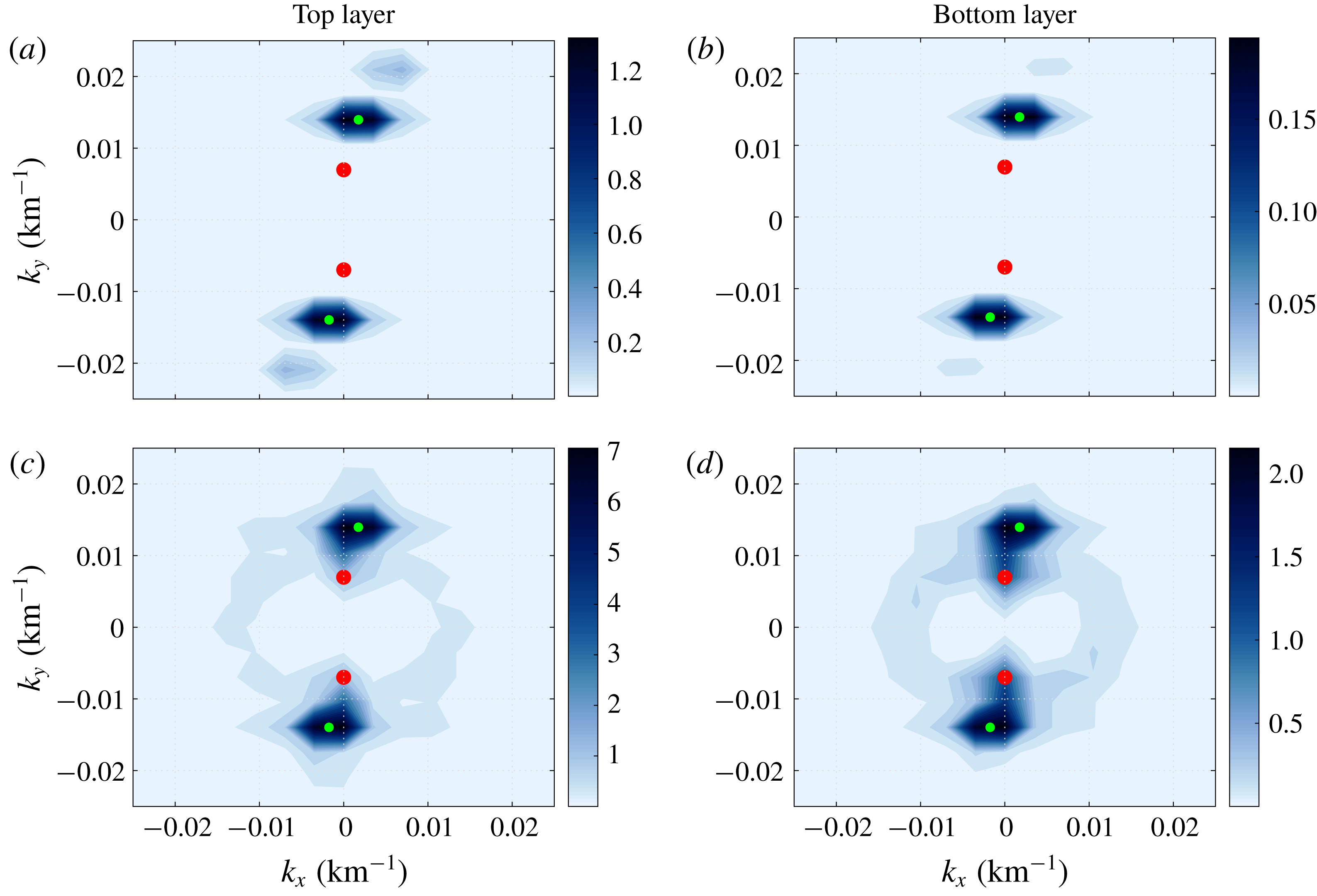
KE spectrum (units are in $\text{cm}^{2}~\text{s}^{-2}$ ) averaged over 2000 days (100 snapshots between 18 000–20 000 days): (a,b) $\unicode[STIX]{x1D708}=200~\text{m}^{2}~\text{s}^{-1}$ and (c,d) $\unicode[STIX]{x1D708}=50~\text{m}^{2}~\text{s}^{-1}$ . Other parameters in the simulations were the same as in table 1. The zonal and meridional wavenumbers are denoted by ( $k_{x}$ , $k_{y}$ ). Green and red dots represent the wavenumbers corresponding to the $J$ and $Z$ modes, respectively. The $Z$ mode seems to receive more energy via nonlinear interactions in the lower eddy viscosity case.

Figure 4.

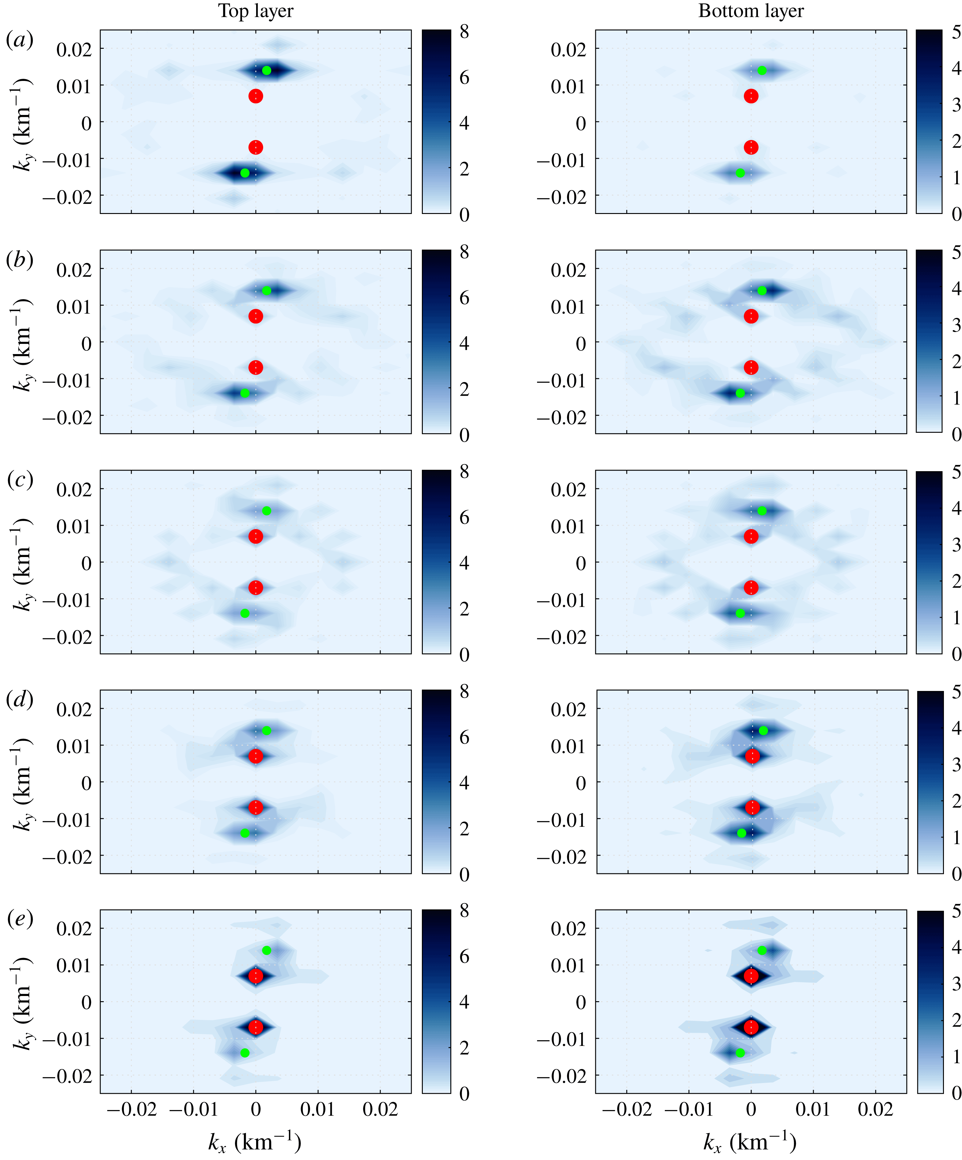
Evolution of the KE spectrum (snapshots, units are in $\text{cm}^{2}~\text{s}^{-2}$ ) after the background flow, eddy viscosity and bottom friction parameters are set to zero. (a–e) KE spectra at 200, 400, 500, 600 and 800 days, respectively. The zonal and meridional wavenumbers are denoted by ( $k_{x}$ , $k_{y}$ ). Green and red dots represent the wavenumbers corresponding to the $J$ and $Z$ modes, respectively.

In order to understand the impacts of eddy viscosity, we first look at the two-dimensional KE spectrum (figure 3). We consider two different solutions with eddy viscosities $200$ and $50~\text{m}^{2}~\text{s}^{-1}$ , respectively. Note that the $Z$ mode is only observed in the latter case (see table 3). From a visual inspection of figure 3, it is quite evident that the $Z$ mode possesses a significant amount of energy in the bottom layer in the lower eddy viscosity case. Another important aspect to note is that many different scales seem to be active in the lower eddy viscosity case (especially in the bottom layer in figure 3). The KE spectra show that, in the lower eddy viscosity case, additional Fourier modes possess significantly more energy than in the higher eddy viscosity case (compare the top and bottom panels in figure 3). These additional Fourier modes are present at relatively smaller spatial scales than the $J$ and $Z$ modes. We hypothesise that these small scales interact with the $J$ mode, which is directly forced by the imposed background shear (Khatri & Berloff Reference Khatri and Berloff2018a ), and feed energy to the $Z$ mode. To confirm this, we ran a test numerical simulation in which the background flow, eddy viscosity and bottom friction parameters were set to zero. We initialised the model using the reference solution from the $\unicode[STIX]{x1D708}=200~\text{m}^{2}~\text{s}^{-1}$ case and the simulation was run for 10 000 days. Figure 4 shows the two-dimensional KE spectra at different times and we observed that many different scales become more energetic. Since the background flow is absent, these additional Fourier modes must have received energy from the $J$ mode through nonlinear interactions because the $J$ mode initially contained most of the energy in the system. Most of the energy is transferred to the $Z$ mode and the $J$ mode almost disappears, as it cannot receive any more energy from the background flow. Here, mesoscale eddies are able to transfer energy to meridional scales even larger than the meridional width of the $J$  mode. This indicates that, in the presence of topography, the meridional width of an alternating jet pattern need not be bounded by the Rhines scale (Rhines Reference Rhines1975), which is set by available eddy energy and Rossby waves in the system. Due to interactions between various large-scale modes, very low meridional wavenumbers can be excited. It is intriguing that the system evolves to purely zonal structures in the case of freely evolving turbulence. It is not yet clear why only zonal patterns emerge and this needs to be further investigated.

Many studies have shown that eddy viscosity has an important role in ocean models (Jochum et al. Reference Jochum, Danabasoglu, Holland, Kwon and Large2008; Arbic et al. Reference Arbic, Polzin, Scott, Richman and Shriver2013). In the geostrophic regime, the viscous term is required to dissipate enstrophy at the grid scale and this goes along with the upscale transfer of energy from mesoscale eddies generated by baroclinic instabilities. However, this is also problematic as a significant amount of energy is also viscously dissipated at small scales and this is not accounted for by the geostrophic turbulence theory (Rhines Reference Rhines1979). This effectively damps out the eddy activity and thus, suppresses the upscale energy transfer by eddies. For eddy viscosity values less than approximately $100~\text{m}^{2}~\text{s}^{-1}$ in our simulations, we observe that oceanic jets, which are initially formed by the action of mesoscale eddies, become unstable and feed energy to even larger flow structures. This eddy viscosity value is not unique and depends on other model parameters, e.g. $U_{b}$ , $\unicode[STIX]{x1D6FD}$ , vertical stratification. The investigation into this upscale energy transfer to meridional scales larger than the Rhines scale (Rhines Reference Rhines1975) has received little attention. We carry out linear stability analysis to study these effects in the next section.

3.2 Wave solutions for $Z$ modes

We find that the propagation velocities of purely zonal $Z$ modes are well predicted by the linear dispersion relation. Also, the flow field is dominated by purely zonal modes in the case of freely evolving turbulence. Here, we derive a simplified expression for the propagation velocity of the $Z$ modes using the linear dispersion relation. Since the contribution from purely zonal modes is at maximum in the absence of forcing and dissipative terms, we set $U_{b}=\unicode[STIX]{x1D708}=\unicode[STIX]{x1D6FE}=0$ in the linear dispersion relation and derive an expression for the meridional phase speed for the $Z$ modes (complete derivation is in appendix B)

(3.2) $$\begin{eqnarray}\displaystyle c_{w}\approx {\displaystyle \frac{\unicode[STIX]{x1D6FD}_{T}(k_{y}^{2}+S_{1})}{k_{y}^{2}(k_{y}^{2}+S_{1}+S_{2})}}, & & \displaystyle\end{eqnarray}$$

where $c_{w}$ and $k_{y}$ are the meridional phase speed and meridional wavenumber, respectively. The meridional velocity of a zonal mode increases linearly with the slope magnitude and decreases roughly as $1/k_{y}^{2}$ (for $k_{y}^{2}\ll S_{1}+S_{2}$ or $k_{y}^{2}\gg S_{1}+S_{2}$ ). This relationship agrees well with the estimates from the nonlinear numerical simulations (see table 2), although the observed propagation speeds differ slightly in magnitude, perhaps, due to the complexity of the flow field.

4 Linear stability analysis in a moving frame of reference

In order to better understand the effects of the eddy viscosity and bottom friction parameters on the stability of the tilted jets ( $J$ mode), we performed a linear stability analysis around the time-mean propagating state of the tilted jets. The approach is similar to the rapid distortion theory (Savill Reference Savill1987). We used a rotated, drifting frame of reference such that the jets are exactly zonal and stationary in it (new axes $(p,q)$ are shown in figure 1 a). Following Khatri & Berloff (Reference Khatri and Berloff2018a ), (2.1) can be rewritten in the new frame of reference as

(4.1) $$\begin{eqnarray}\displaystyle & & \displaystyle \displaystyle \left[{\displaystyle \frac{\unicode[STIX]{x2202}}{\unicode[STIX]{x2202}t}}-c{\displaystyle \frac{\unicode[STIX]{x2202}}{\unicode[STIX]{x2202}q}}\right]\unicode[STIX]{x1D6F1}_{i}+\left({\displaystyle \frac{\unicode[STIX]{x2202}\unicode[STIX]{x1D713}_{i}}{\unicode[STIX]{x2202}p}}-\unicode[STIX]{x1D6FF}_{i1}U_{b}\sin \unicode[STIX]{x1D703}\right){\displaystyle \frac{\unicode[STIX]{x2202}\unicode[STIX]{x1D6F1}_{i}}{\unicode[STIX]{x2202}q}}-\left({\displaystyle \frac{\unicode[STIX]{x2202}\unicode[STIX]{x1D713}_{i}}{\unicode[STIX]{x2202}q}}-\unicode[STIX]{x1D6FF}_{i1}U_{b}\cos \unicode[STIX]{x1D703}\right){\displaystyle \frac{\unicode[STIX]{x2202}\unicode[STIX]{x1D6F1}_{i}}{\unicode[STIX]{x2202}p}}\nonumber\\ \displaystyle & & \displaystyle \displaystyle \quad =\unicode[STIX]{x1D708}\unicode[STIX]{x1D6FB}^{4}\unicode[STIX]{x1D713}_{i}-\unicode[STIX]{x1D6FF}_{i2}\unicode[STIX]{x1D6FE}\unicode[STIX]{x1D6FB}^{2}\unicode[STIX]{x1D713}_{i},\end{eqnarray}$$

where

(4.2) $$\begin{eqnarray}\displaystyle \left.\begin{array}{@{}rcl@{}}\displaystyle \unicode[STIX]{x1D6F1}_{1}\ & =\ & \unicode[STIX]{x1D6FB}^{2}\unicode[STIX]{x1D713}_{1}+S_{1}(\unicode[STIX]{x1D713}_{2}-\unicode[STIX]{x1D713}_{1})+(\unicode[STIX]{x1D6FD}+S_{1}U_{b})(q\cos \unicode[STIX]{x1D703}+p\sin \unicode[STIX]{x1D703}+ct\cos \unicode[STIX]{x1D703}),\\ \displaystyle \unicode[STIX]{x1D6F1}_{2}\ & =\ & \unicode[STIX]{x1D6FB}^{2}\unicode[STIX]{x1D713}_{2}+S_{2}(\unicode[STIX]{x1D713}_{1}-\unicode[STIX]{x1D713}_{2})+(\unicode[STIX]{x1D6FD}-S_{2}U_{b})(q\cos \unicode[STIX]{x1D703}+p\sin \unicode[STIX]{x1D703}+ct\cos \unicode[STIX]{x1D703})\\ \ & \ & +\,\unicode[STIX]{x1D6FD}_{T}(-q\sin \unicode[STIX]{x1D703}+p\cos \unicode[STIX]{x1D703}-ct\sin \unicode[STIX]{x1D703}).\end{array}\right\} & & \displaystyle\end{eqnarray}$$

Here, $\unicode[STIX]{x1D6FF}_{ij}$ is the Kronecker delta. The tilt angle, $\unicode[STIX]{x1D703}$ , and drift speed of the frame of reference, $c$ , are estimated from the EOF analysis. We linearise the governing equations around the time-mean tilted jets and represent the streamfunction as a sum of the mean and perturbation terms $\unicode[STIX]{x1D713}_{i}(p,q,t)=\overline{\unicode[STIX]{x1D713}}_{i}(q)+\unicode[STIX]{x1D713}_{i}^{\prime }(p,q,t)$ . We substitute the decomposed $\unicode[STIX]{x1D713}_{i}$ in (4.1), and the final equation in terms of $\unicode[STIX]{x1D713}_{i}^{\prime }$ is (see the full derivation in appendix D)

(4.3) $$\begin{eqnarray}\displaystyle & & \displaystyle \displaystyle {\displaystyle \frac{\unicode[STIX]{x2202}}{\unicode[STIX]{x2202}t}}[\unicode[STIX]{x1D6FB}^{2}\unicode[STIX]{x1D713}_{i}^{\prime }+\unicode[STIX]{x1D716}_{i}S_{i}(\unicode[STIX]{x1D713}_{2}^{\prime }-\unicode[STIX]{x1D713}_{1}^{\prime })]+\left[A_{i}{\displaystyle \frac{\unicode[STIX]{x2202}}{\unicode[STIX]{x2202}p}}+B_{i}{\displaystyle \frac{\unicode[STIX]{x2202}}{\unicode[STIX]{x2202}q}}\right][\unicode[STIX]{x1D6FB}^{2}\unicode[STIX]{x1D713}_{i}^{\prime }+\unicode[STIX]{x1D716}_{i}S_{i}(\unicode[STIX]{x1D713}_{2}^{\prime }-\unicode[STIX]{x1D713}_{1}^{\prime })]\nonumber\\ \displaystyle & & \displaystyle \displaystyle \quad +\,C_{i}{\displaystyle \frac{\unicode[STIX]{x2202}\unicode[STIX]{x1D713}_{i}^{\prime }}{\unicode[STIX]{x2202}p}}+D_{i}{\displaystyle \frac{\unicode[STIX]{x2202}\unicode[STIX]{x1D713}_{i}^{\prime }}{\unicode[STIX]{x2202}q}}=\unicode[STIX]{x1D708}\unicode[STIX]{x1D6FB}^{4}\unicode[STIX]{x1D713}_{i}^{\prime }-\unicode[STIX]{x1D6FF}_{i2}\unicode[STIX]{x1D6FE}\unicode[STIX]{x1D6FB}^{2}\unicode[STIX]{x1D713}_{i}^{\prime },\end{eqnarray}$$

and

(4.4) $$\begin{eqnarray}\displaystyle \left.\begin{array}{@{}l@{}}\displaystyle A_{1}=U_{b}\cos \unicode[STIX]{x1D703}+\overline{u}_{1},\\ A_{2}=\overline{u}_{2},\\ \displaystyle B_{1}=-c-U_{b}\sin \unicode[STIX]{x1D703},\\ B_{2}=-c,\\ \displaystyle C_{1}=(\unicode[STIX]{x1D6FD}+S_{1}U_{b})\cos \unicode[STIX]{x1D703}-\overline{u}_{1}^{\prime \prime }+S_{1}(\overline{u}_{1}-\overline{u}_{2}),\\ \displaystyle C_{2}=(\unicode[STIX]{x1D6FD}-S_{2}U_{b})\cos \unicode[STIX]{x1D703}-\unicode[STIX]{x1D6FD}_{T}\sin \unicode[STIX]{x1D703}-\overline{u}_{2}^{\prime \prime }+S_{2}(\overline{u}_{2}-\overline{u}_{1}),\\ \displaystyle D_{1}=-(\unicode[STIX]{x1D6FD}+S_{1}U_{b})\sin \unicode[STIX]{x1D703},\\ D_{2}=-(\unicode[STIX]{x1D6FD}-S_{2}U_{b})\sin \unicode[STIX]{x1D703}-\unicode[STIX]{x1D6FD}_{T}\cos \unicode[STIX]{x1D703}.\end{array}\right\} & & \displaystyle\end{eqnarray}$$

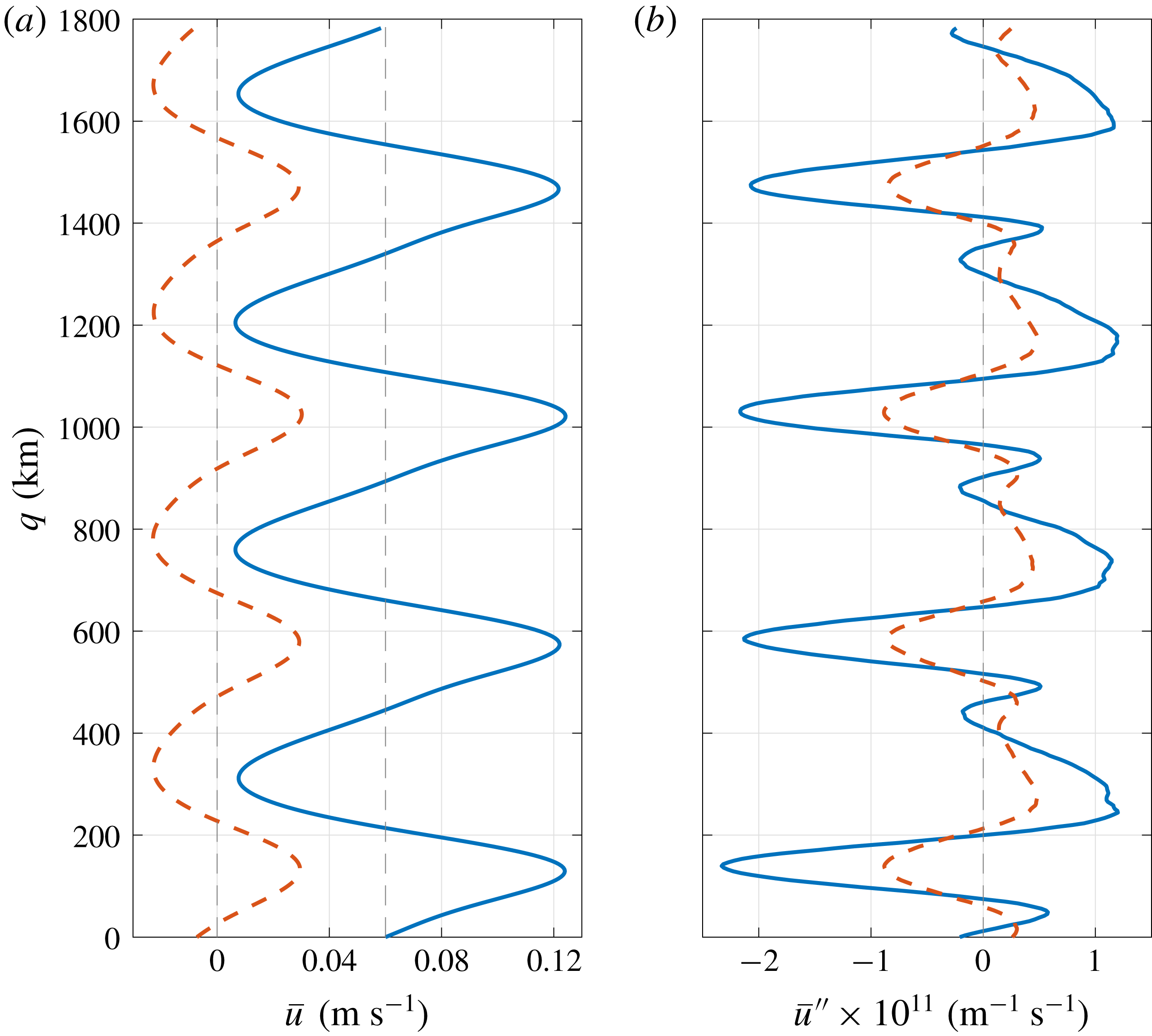
Here, $\overline{u}_{i}=-(\unicode[STIX]{x2202}\overline{\unicode[STIX]{x1D713}}_{i}/\unicode[STIX]{x2202}q)$ and $\overline{u}_{i}^{\prime \prime }$ are the mean (averaged in $p$ direction) flow and its double derivative in $q$ direction, respectively (shown in figure 5). We computed $\overline{\unicode[STIX]{x1D713}}_{i}(q)$ by averaging the streamfunction field over time for the last 10 000 days in the moving frame of reference and then averaging along the direction $p$ . We used the data from the simulation corresponding to figure 1.

Figure 5.

Profiles of $\overline{u}_{i}$ and $\overline{u}_{i}^{\prime \prime }$ used in the stability analysis. The profiles were computed by applying spatial averaging in the direction along with the jets in the moving frame of reference between 10 000 and 20 000 days for the simulation corresponding to figure 1 (blue solid line in the top layer and red dotted line in the bottom layer). The velocity profile in the top layer is shown relative to the imposed background flow of $0.06~\text{m}~\text{s}^{-1}$ .

The system of equations (4.3) can be solved as the coefficients ( $A_{i}$ , $B_{i}$ , $C_{i}$ , $D_{i}$ ) are known, and the only unknown parameters are $\unicode[STIX]{x1D713}_{1}^{\prime }$ and $\unicode[STIX]{x1D713}_{2}^{\prime }$ . For this purpose, periodic boundary conditions were imposed on all four sides of the domain, with Fourier decomposition in $p$ direction, i.e. along with the jets, and finite-difference discretisation in $q$ direction. We assumed solutions of the kind $\unicode[STIX]{x1D713}_{i}^{\prime }=\tilde{\unicode[STIX]{x1D713}_{i}}(q)\text{e}^{\text{i}(lp-\unicode[STIX]{x1D714}t)}$ for the perturbation terms ( $l$ is the wavenumber in the direction along with the tilted jets), which results in an eigenvalue problem. This is similar to the method discussed in Berloff et al. (Reference Berloff, Karabasov, Farrar and Kamenkovich2011), Berloff & Kamenkovich (Reference Berloff and Kamenkovich2013a ), but in the presence of topography. The eigenvalue problem was solved for each wavenumber $l$ separately, and the analysis was repeated for different magnitudes of the eddy viscosity and bottom friction parameters (details are in appendix D).

Figure 6.

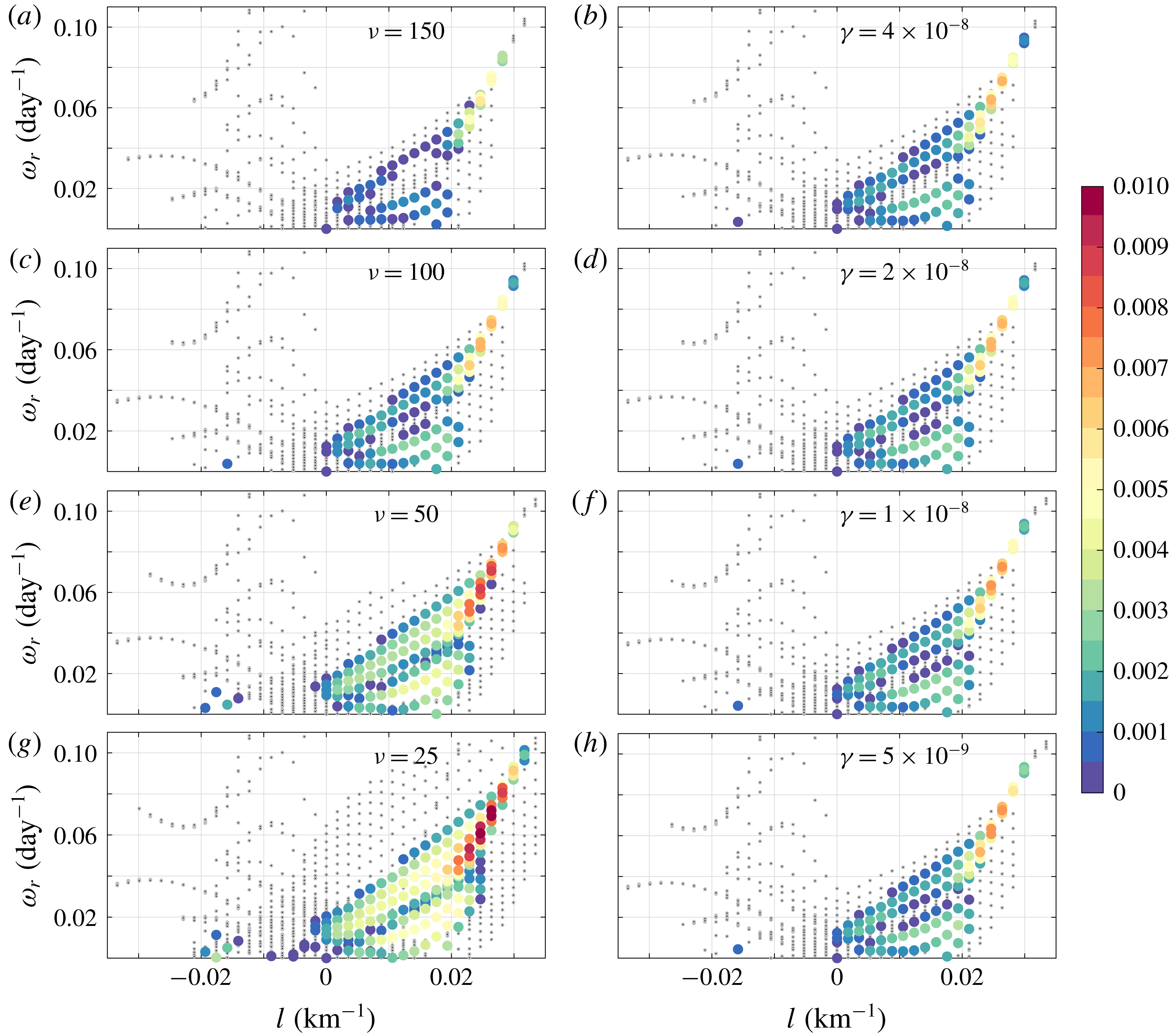
Real parts of eigenvalues ( $\unicode[STIX]{x1D714}_{r}$ ) obtained from the linear stability analysis for different values of eddy viscosity ((a,c,e,g), for fixed $\unicode[STIX]{x1D6FE}=2\times 10^{-8}~\text{s}^{-1}$ ) and bottom friction ((b,d,f,h), for fixed $\unicode[STIX]{x1D708}=100~\text{m}^{2}~\text{s}^{-1}$ ) versus wavenumber. Growth rates ( $\text{day}^{-1}$ ) are shown in the colour bar. Eigenmodes having growth rates in the range [ $-0.01,0$ ] are shown with grey dots. Growth rates increase with decreasing $\unicode[STIX]{x1D708}$ and $\unicode[STIX]{x1D6FE}$ .

In figure 6, frequencies obtained by solving the eigenvalue problem are plotted against $l$ for different magnitudes of the eddy viscosity and bottom friction parameters. It is evident that eddy viscosity tends to stabilise the eigenmodes at all wavenumbers as the growth rates are smaller for higher eddy viscosity values at the same wavenumbers. In fact, in the lower viscosity cases, many weakly unstable large-scale modes appear, which otherwise had negative growth rates. In the case of bottom friction, the changes in the growth rates are less visible, but the growth rates do increase with decreasing $\unicode[STIX]{x1D6FE}$ . A few unstable modes can be seen appearing in the cases of weaker bottom friction (compare plots for $\unicode[STIX]{x1D6FE}=4\times 10^{-8}$ and $\unicode[STIX]{x1D6FE}=2\times 10^{-8}~\text{s}^{-1}$ ). 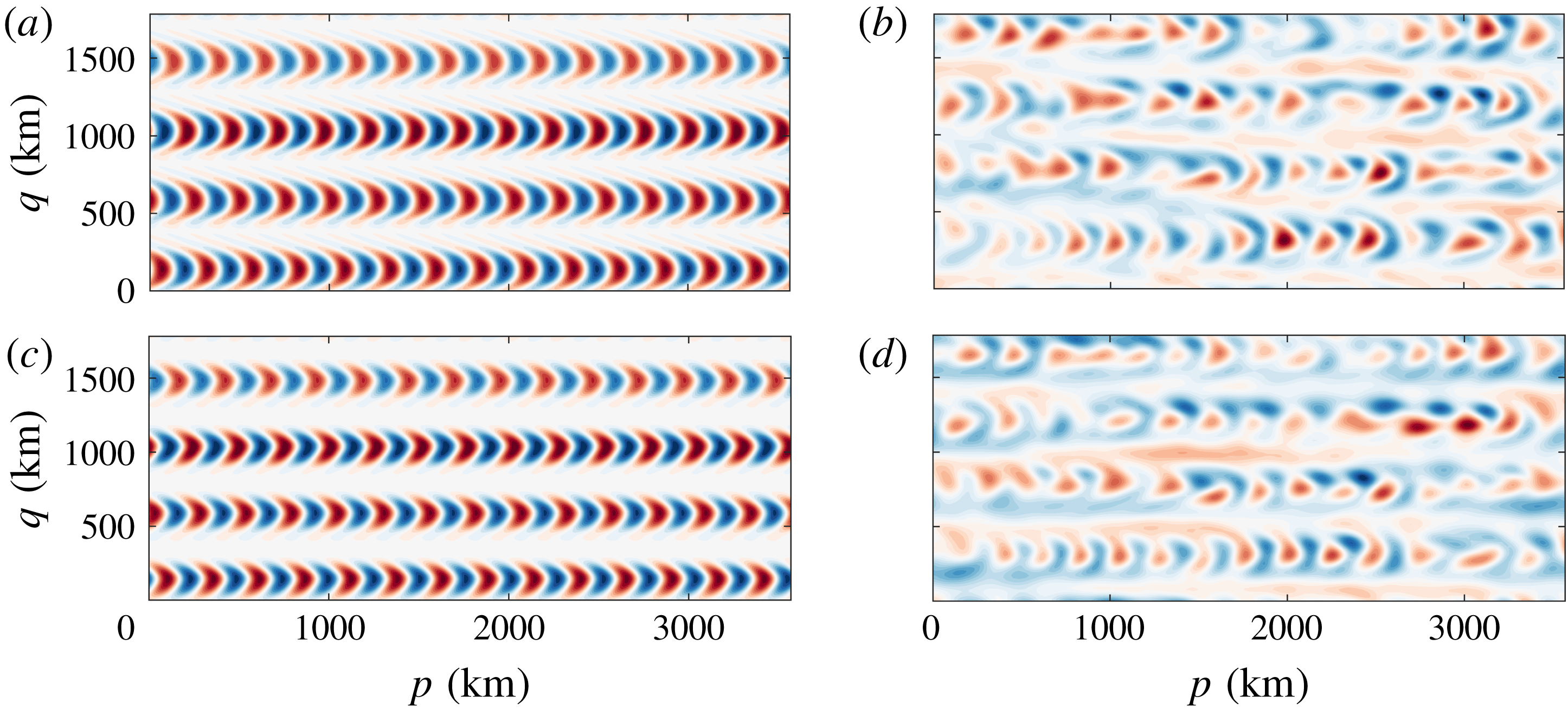Also, we did not observe the $Z$ mode in the numerical simulation run with $\unicode[STIX]{x1D6FE}=4\times 10^{-8}~\text{s}^{-1}$ (table 4). Looking at the spatial structure of the fastest growing mode (figure 7), we found that the banana-shaped eddies are very similar to the eigenfunctions corresponding to the fastest growing mode in a flat-bottom case (see figure 13 in Berloff et al. (Reference Berloff, Karabasov, Farrar and Kamenkovich2011)). In fact, the banana-shaped eigenmode matches very well with the eddy field reconstructed using all EOFs except the EOFs corresponding to $J$ mode.

Figure 7.

(a,c) The eigenvector corresponding to the fastest growing mode, (b,d) snapshots of the eddy field constructed using all EOFs except EOF 1-2 ((a,b) and (c,d) represent the top and bottom layers, respectively). The snapshot of eddy field is from the numerical simulation where $\unicode[STIX]{x1D708}=150~\text{m}^{2}~\text{s}^{-1}$ was used (other parameters – refer to caption in figure 2). In this case, there is a remarkable resemblance in the spatial structure between the eddy field and the fastest growing eigenfunction. In the lower viscosity simulation (e.g. $\unicode[STIX]{x1D708}=100~\text{m}^{2}~\text{s}^{-1}$ ), these banana-shaped structures appear less frequently because the eddy field is very complex in the presence of the $Z$ mode.

Given very small growth rates of modes at relatively large scales, energy must have been transferred to the $Z$ mode through nonlinear interactions among different eigenmodes, which can be inferred from KE spectrum in figure 4. The linear stability analysis shows that the eigenmodes are significantly damped due to eddy viscosity and there are fewer unstable modes present in the case of strong eddy viscosity. Consequently, the number of nonlinear interactions can be reduced due to the presence of fewer energised eigenmodes, and the efficiency of energy exchange among different eigenmodes can decline. This suggests that nonlinear interactions may have been suppressed in the simulations having strong dissipation, which can explain the absence of the $Z$ modes in the EOF analysis in some cases (see table 3 for $\unicode[STIX]{x1D708}=150,200~\text{m}^{2}~\text{s}^{-1}$ cases). There may not have been enough interactions to feed energy to the $Z$ modes. It is possible that strong viscous dissipation reduces these nonlinear interactions by damping out the small scales.

It is counterintuitive that, in the presence of topography, mesoscale eddies are actually able to transfer energy to zonally elongated modes that have meridional wavelengths longer than the meridional width of the tilted jets. Over a flat bottom, the $\unicode[STIX]{x1D6FD}$ -effect leads to strong anisotropisation resulting in the formation of zonal jets, where the meridional width of the jets is set by a balance between nonlinear advection and Rossby waves (Rhines Reference Rhines1975). It would be wrong to expect that Rossby waves directly inhibit the inverse energy transfer to meridional scales longer than the Rhines scale (Sukoriansky, Dikovskaya & Galperin Reference Sukoriansky, Dikovskaya and Galperin2007). The upscale energy transfer stops at the Rhines scale because, in order to transfer energy to lower meridional wavenumbers, triad interactions would involve two almost parallel Fourier modes and such triad interactions are quite inefficient (Vallis & Maltrud Reference Vallis and Maltrud1993). On the other hand, in the presence of topography, both zonal and tilted large-scale Fourier modes are present, as seen in the two-dimensional KE spectra and linear stability analysis. Given that various Fourier modes at low wavenumbers are sufficiently energetic and are not parallel, it is possible for these Fourier modes to have efficient triad interactions and transfer energy to very low meridional wavenumbers. This could be the main reason why the $Z$ mode is able to receive a significant amount of energy in the simulations. It may be possible to test this hypothesis directly. One could try to identify the triads in which the $Z$ mode gains energy or the $J$ mode loses energy and compute the energy exchange rates as a function of the magnitudes of the eddy viscosity and bottom friction parameters. Identifying all such triads is a challenging task and this is beyond the scope of this paper.