1 Introduction
Nonlinear interactions between waves and suitably defined mean flows have long been studied in fluid mechanics, with early examples focusing on acoustic streaming and related effects (e.g. Lighthill Reference Lighthill1978). The field underwent a dramatic extension and deepening in the second half of the last century, when the crucial importance of such interactions for the long-term dynamics of the atmosphere and oceans was realized (as detailed in textbooks such as Andrews, Holton & Leovy Reference Andrews, Holton and Leovy1987; Vallis Reference Vallis2006). By now, wave–mean interaction theory has become a mature field with solid theoretical foundations (e.g. Bühler Reference Bühler2014).
Much of the original wave–mean interaction theory was developed for a situation in which small-amplitude waves are propagating on a non-uniform but laminar basic flow of much larger amplitude (Eliassen & Palm Reference Eliassen and Palm1961). This is a natural model for atmospheric internal waves propagating on a basic state characterized by a strong jet stream, for example. The Eulerian averaging operation that defines the mean flow can then be chosen as large-scale zonal averaging along latitude circles. Mathematically, the situation is described by a perturbation expansion in a small-amplitude parameter
 $a\ll 1$
in terms of which the basic flow is
 $O(1)$
and the wave-like disturbances are
 $O(a)$
. Nonlinear effects such as wave-induced changes in the mean flow then accrue at
 $O(a^{2})$
and those are obviously small changes of the
 $O(1)$
basic state. Significant changes of the basic state are then possible only if there are resonant mean-flow responses that grow as
 $O(a^{2}t)$
in time
 $t$
. For a steady wave field on a laminar flow, the non-acceleration theorem then shows this is only possible if the waves are dissipating or breaking in some location, which led to the well-established theory of dissipative wave drag and critical layers described in the textbooks cited above. In this connection the natural slow time scale for significant mean-flow changes to occur is
 $t=O(a^{-2})$
, as exemplified by the classical theory of the quasi-biennial oscillation in the equatorial lower stratosphere in Plumb (Reference Plumb1977).
However, present-day research in atmosphere–ocean fluid dynamics has pushed to smaller spatial scales, where the amplitude of the mean flow is not necessarily larger than that of the waves. A prime example of this is the so-called submesoscale regime in oceanography, which is often characterized by horizontal scales significantly below the deformation radius. At these scales of less than 100 km the relevant mean flow is naturally defined by its slowness when compared to fast wave motions, i.e. the natural Eulerian averaging operation that now defines the mean flow is a slowly varying time average. Of course, such a mean flow is now three-dimensional and itself unsteady, which is a significant departure from the classical theory based on zonal averaging.
For example, a problem of considerable contemporary interest in oceanography concerns the long-term consequences of the interactions between storm-generated near-inertial oscillations and the much slower geostrophically balanced mean flow (e.g. Alford et al. Reference Alford, MacKinnon, Simmons and Nash2016). In this physical situation the waves are of comparable magnitude or even larger than the balanced mean flow, which makes the earlier theory based on strong mean flows less relevant. Again, there is no obvious spatial scale separation between waves and mean flows in this situation, so time averaging over the fast wave oscillations is the only option to define the mean flow.
Rigorous general results, i.e. results with rigorous error control, are sparse in this area. With periodic boundary conditions, the particular case where waves and balanced flow are both
 $O(a)$
is amenable to rigorous two-timing analysis in spectral space (Babin, Mahalov & Nicolaenko Reference Babin, Mahalov and Nicolaenko1997; Majda & Embid Reference Majda and Embid1998), with a sub-linear growth solvability condition that determines the evolution on the first nonlinear slow time scale
 $t=O(a^{-1})$
. In the presence of significant Coriolis forces, the main result from these studies has been that the interactions are weak, with no significant energy exchanges between waves and quasi-geostrophic mean flows on this time scale. However, it has not been possible to extend this rigorous multi-scale analysis to the second slow time scale
 $t=O(a^{-2})$
, which would have been of primary interest in classical wave–mean interaction theory. A discussion of the difficulties involved is given in § 6 in Bühler (Reference Bühler2000).
In the absence of a rigorous general theory to push to the longer time scale, research in this area has focused on theoretical and numerical case studies of various particular interaction scenarios. An important theme that has emerged in this connection is the notion of a modified diagnostic relation between the streamfunction describing the balanced mean flow and the materially advected potential vorticity (PV). This modification consists of certain wave-induced terms, such as the vertical curl of the horizontal pseudomomentum vector, that must be added to the standard quasi-geostrophic terms to obtain long-time accuracy for the mean flow. The relevance of such modified diagnostic relations was already implied in the landmark paper of Bretherton (Reference Bretherton1969), who computed the
 $O(a^{2})$
mean-flow response to compactly supported three-dimensional and two-dimensional wavepackets in the non-rotating Boussinesq equations (see van den Bremer & Sutherland (Reference van den Bremer and Sutherland2014) for a recent extension of this work to higher accuracy and Wagner & Young (Reference Wagner and Young2015) for further extension both in wave amplitude and in treating a rotating Boussinesq flow). A general derivation and description of the modified diagnostic relation concept was first presented in Bühler & McIntyre (Reference Bühler and McIntyre1998) (hereafter BM98), using rotating shallow-water and three-dimensional Boussinesq flows.
The modified diagnostic relation concept arises naturally in recent studies of the near-inertial wave problem (e.g. Xie & Vanneste Reference Xie and Vanneste2015; Wagner & Young Reference Wagner and Young2016; Thomas, Smith & Bühler Reference Thomas, Smith and Bühler2017). In this connection, the present authors have recently investigated numerically over very long time periods various cases of interactions between small-amplitude inertia–gravity waves and balanced mean flows in the rotating shallow-water equations. Here the waves and the PV field overlapped in spatial scale, the wave amplitude was
 $O(a)$
and the PV amplitude was either
 $O(a)$
or smaller (manuscript in preparation). If the PV amplitude is so weak that it can be taken to be zero one obtains the rigorous constraint that the PV is uniform throughout and equal to its background value always and everywhere. Significant theoretical progress beyond numerical experimentation can be made in this limiting case, and this is the topic of the present paper.
To this end we formulate the equations for the complete
 $O(a^{2})$
mean-flow response induced by
 $O(a)$
waves on a uniform PV background in rotating shallow water, which extends and in one place corrects previous work on the subject in BM98. We then study the solution to these equations first in the context of slowly varying wave fields, such as a steady wavetrain or unsteady wavepackets, and second in the case of a monochromatic standing wave. The latter case is motivated by the prevalence of nearly monochromatic internal tides in the ocean (e.g. Garrett & Kunze Reference Garrett and Kunze2007), which are not slowly varying waves in space. Detailed theoretical predictions are obtained for these cases, which are subsequently checked and illustrated by independent direct numerical simulations of the full nonlinear shallow-water equations.
Notably, we do not assume that the mean flow is balanced in our computations, i.e. we allow for a full
 $O(a^{2})$
mean-flow response, which itself can contain wave-like motions. This is different from studies such as Wagner & Young (Reference Wagner and Young2015) or Xie & Vanneste (Reference Xie and Vanneste2015), where detailed mean-flow results were obtained but only under the assumption that the mean flow was balanced. In particular, we will investigate dynamical processes that unfold on the intermediate time scale for wave–wave interactions that was explicitly omitted in Wagner & Young (Reference Wagner and Young2015), as discussed in their § 4.2 on the set-up for the two-timing asymptotics. Moreover, as we do not assume that the mean flow is balanced, we are able to derive theoretical and numerical results for a wide range of
 $f$
, from weak to strong rotation.
We pay particular attention to the errors in the mean-flow computation that would result from ignoring the intrinsic time dependence of propagating wavepackets, and we also investigate the overall magnitude of the mean-flow response as a function of the Coriolis parameter
 $f$
. We find that for very large
 $f$
the mean-flow response is typically ‘choked’ and decays quickly with
 $f$
, but we also show by way of an explicit counterexample using standing waves that the strongest mean-flow response is not always reached in the non-rotating limit
 $f=0$
.
The plan for the paper is as follows: the governing equations are developed in § 2 and their relevant form for slowly varying waves is discussed in detail in § 3 for both steady wavetrains and propagating wavetrains. The alternative scenario of monochromatic standing waves is developed in § 4, direct numerical simulations are presented in § 5 and concluding remarks are offered in § 6.
Finally, we prefer to use Lagrangian-mean velocity as a natural field with which to describe the mean flow, but we avoid using the full machinery of generalized Lagrangian-mean theory (GLM) by deriving the
 $O(a^{2})$
equations using elementary methods. It would have been shorter to simply refer to the relevant equations in Andrews & McIntyre (Reference Andrews and McIntyre1978) (hereafter AM78a), but in this way the present paper is more self-contained.
2 Governing equations
We consider the rotating shallow-water equations on flat topography:
 $$\begin{eqnarray}\frac{\text{D}\boldsymbol{u}}{\text{D}t}+\boldsymbol{f}\times \boldsymbol{u}+g\unicode[STIX]{x1D735}h=0\quad \text{and}\quad \frac{\text{}\unicode[STIX]{x2202}\text{}h}{\text{}\unicode[STIX]{x2202}\text{}t}+\unicode[STIX]{x1D735}\boldsymbol{\cdot }(h\boldsymbol{u})=0.\end{eqnarray}$$
Here
 $\boldsymbol{u}=(u,v)$
is the velocity,
 $\text{D}/\text{D}t=\unicode[STIX]{x2202}_{t}+(\boldsymbol{u}\boldsymbol{\cdot }\unicode[STIX]{x1D735})$
is the material derivative,
 $\boldsymbol{f}=f\widehat{\boldsymbol{z}}$
is the constant Coriolis vector,
 $h$
is the layer depth and
 $g$
is gravity. The associated PV
 $$\begin{eqnarray}q=\frac{\unicode[STIX]{x1D735}\times \boldsymbol{u}+f}{h}\quad \text{such that}\quad \frac{\text{D}q}{\text{D}t}=0\end{eqnarray}$$
holds for smooth flows, i.e. flows without shocks. Here
 $\unicode[STIX]{x1D735}\times \boldsymbol{u}$
is shorthand for
 $\widehat{\boldsymbol{z}}\boldsymbol{\cdot }(\unicode[STIX]{x1D735}\times \boldsymbol{u})$
.
Throughout this paper we assume that
 $q$
is uniform and equal to its background value
 $f/H$
, where
 $H$
is the undisturbed layer depth. The material invariance of
 $q$
implies that this will remain the case as long as the flow evolves smoothly in time. We therefore have the global vortex stretching constraint
 $$\begin{eqnarray}q=\frac{f}{H}\quad \Leftrightarrow \quad \unicode[STIX]{x1D735}\times \boldsymbol{u}=\frac{h-H}{H}\,f.\end{eqnarray}$$
2.1 Linear wave perturbations
We assume that the entire flow is a weak perturbation to the rest state
 $\boldsymbol{u}=0$
and
 $h=H$
. Specifically, we introduce a small-amplitude parameter
 $a\ll 1$
and pursue a regular perturbation expansion in powers of
 $a$
. The linear perturbations
 $(\boldsymbol{u}^{\prime },h^{\prime })=O(a)$
satisfy the usual linear equations
 $$\begin{eqnarray}\frac{\text{}\unicode[STIX]{x2202}\text{}\boldsymbol{u}^{\prime }}{\text{}\unicode[STIX]{x2202}\text{}t}+\boldsymbol{f}\times \boldsymbol{u}^{\prime }+g\unicode[STIX]{x1D735}h^{\prime }=0\quad \text{and}\quad \frac{\text{}\unicode[STIX]{x2202}\text{}h^{\prime }}{\text{}\unicode[STIX]{x2202}\text{}t}+H\unicode[STIX]{x1D735}\boldsymbol{\cdot }\boldsymbol{u}^{\prime }=0.\end{eqnarray}$$
The corresponding linear PV
 $$\begin{eqnarray}q^{\prime }=\unicode[STIX]{x1D735}\times \boldsymbol{u}^{\prime }-\frac{h^{\prime }}{H}f=0\end{eqnarray}$$
by (2.3). Hence the linear dynamics is described entirely by the inertia–gravity wave modes of the system, as the balanced vortical mode is zero. In particular, plane waves with wavenumber
 $\boldsymbol{k}=(k,l)$
and frequency
 $\hat{\unicode[STIX]{x1D714}}$
satisfy the dispersion relation
 $$\begin{eqnarray}\hat{\unicode[STIX]{x1D714}}^{2}=f^{2}+c^{2}(k^{2}+l^{2})\quad \text{where}\quad \!\!c^{2}=gH.\end{eqnarray}$$
The governing equation for the wave energy density
 $$\begin{eqnarray}E=\frac{1}{2}\left(\overline{{u^{\prime }}^{2}}+\overline{{v^{\prime }}^{2}}+\frac{g}{H}\overline{{h^{\prime }}^{2}}\right)\end{eqnarray}$$
follows from (2.4) as
 $$\begin{eqnarray}\frac{\text{}\unicode[STIX]{x2202}\text{}E}{\text{}\unicode[STIX]{x2202}\text{}t}+\unicode[STIX]{x1D735}\boldsymbol{\cdot }(g\overline{h^{\prime }\boldsymbol{u}^{\prime }})=0.\end{eqnarray}$$
Here we introduced a suitable Eulerian averaging operator
 $\overline{(\ldots )}$
that commutes with
 $\unicode[STIX]{x2202}_{t}$
and
 $\unicode[STIX]{x1D735}$
and acts like a linear projection in the sense that
 $\overline{h^{\prime }}=0$
and so on. The precise nature of the averaging operator does not affect the general theory in this section, but specific results will subsequently be based on phase averages over wave oscillations. The wave energy
 $E$
is an example of a second-order wave property in the sense that
 $E=O(a^{2})$
, yet it can be evaluated from the linear,
 $O(a)$
solution alone. Other wave properties of interest include the
 $O(a^{2})$
Stokes corrections
 $$\begin{eqnarray}\overline{\boldsymbol{u}}^{S}=\overline{(\unicode[STIX]{x1D743}^{\prime }\boldsymbol{\cdot }\unicode[STIX]{x1D735})\boldsymbol{u}^{\prime }}\quad \text{and}\quad \overline{h}^{S}=\overline{(\unicode[STIX]{x1D743}^{\prime }\boldsymbol{\cdot }\unicode[STIX]{x1D735})h^{\prime }}.\end{eqnarray}$$
Here
 $\unicode[STIX]{x1D743}^{\prime }$
is the linear particle displacement defined by
 $$\begin{eqnarray}\frac{\text{}\unicode[STIX]{x2202}\text{}\unicode[STIX]{x1D743}^{\prime }}{\text{}\unicode[STIX]{x2202}\text{}t}=\boldsymbol{u}^{\prime }\quad \text{and}\quad \overline{\unicode[STIX]{x1D743}^{\prime }}=0.\end{eqnarray}$$
The field
 $\overline{\boldsymbol{u}}^{S}$
is commonly known as the Stokes drift, and generically
 $\overline{\unicode[STIX]{x1D719}}^{S}=\overline{(\unicode[STIX]{x1D743}^{\prime }\boldsymbol{\cdot }\unicode[STIX]{x1D735})\unicode[STIX]{x1D719}^{\prime }}$
denotes the leading-order Stokes correction to any field
 $\unicode[STIX]{x1D719}$
. With
 $\unicode[STIX]{x1D743}^{\prime }$
in hand the linear continuity equation in (2.4) can be integrated to
 $$\begin{eqnarray}h^{\prime }=-H\unicode[STIX]{x1D735}\boldsymbol{\cdot }\unicode[STIX]{x1D743}^{\prime }.\end{eqnarray}$$
Also, taking the dot product of
 $\unicode[STIX]{x1D743}^{\prime }$
with the linear momentum equation in (2.4), averaging and integrating by parts in time yields the
 $O(a^{2})$
virial theorem (cf. AM78a)
 $$\begin{eqnarray}\frac{1}{2}\frac{\text{}\unicode[STIX]{x2202}^{2}\text{}}{\text{}\unicode[STIX]{x2202}\text{}t^{2}}\overline{|\unicode[STIX]{x1D743}^{\prime }|^{2}}+g\overline{h}^{S}=\overline{\boldsymbol{u}^{\prime }\boldsymbol{\cdot }(\boldsymbol{u}^{\prime }+\boldsymbol{f}\times \unicode[STIX]{x1D743}^{\prime })}.\end{eqnarray}$$
A key wave property for wave–mean interaction theory is the
 $O(a^{2})$
Lagrangian-mean pseudomomentum vector
 $\boldsymbol{p}$
(AM78a) whose Cartesian components are
 $$\begin{eqnarray}p_{i}=-\overline{\unicode[STIX]{x1D709}_{j,i}^{\prime }\left(u_{j}^{\prime }+\textstyle \frac{1}{2}\unicode[STIX]{x1D716}_{jkm}f_{k}\unicode[STIX]{x1D709}_{m}^{\prime }\right)}.\end{eqnarray}$$
Here the summation convention is used, the comma denotes spatial derivatives and
 $\unicode[STIX]{x1D716}_{jkm}$
is the Levi-Civita symbol. The evolution law for
 $\boldsymbol{p}$
follows from contracting the
 $j$
th component of the linear momentum equation with
 $-\unicode[STIX]{x1D709}_{j,i}^{\prime }$
and averaging. This yields
 $$\begin{eqnarray}\frac{\text{}\unicode[STIX]{x2202}\text{}p_{i}}{\text{}\unicode[STIX]{x2202}\text{}t}+\overline{\left(\frac{1}{2}u_{j}^{\prime }\left(u_{j}^{\prime }+\unicode[STIX]{x1D716}_{jkm}f_{k}\unicode[STIX]{x1D709}_{m}^{\prime }\right)\right)}_{,i}=g\overline{\unicode[STIX]{x1D709}_{j,i}^{\prime }h_{,j}^{\prime }}=\left(g\overline{\unicode[STIX]{x1D709}_{j,i}^{\prime }h^{\prime }}+\frac{g\overline{{h^{\prime }}^{2}}}{2H}\unicode[STIX]{x1D6FF}_{ji}\right)_{,j},\end{eqnarray}$$
where the latter divergence form makes obvious that this is a conservation law for
 $\boldsymbol{p}$
. The manipulations leading to (2.14) are straightforward except for the treatment of the Coriolis term, which is decomposed as
 $$\begin{eqnarray}-\unicode[STIX]{x1D709}_{j,i}^{\prime }\unicode[STIX]{x1D716}_{jkm}f_{k}u_{m}^{\prime }=-\frac{1}{2}\frac{\text{}\unicode[STIX]{x2202}\text{}}{\text{}\unicode[STIX]{x2202}\text{}t}(\unicode[STIX]{x1D709}_{j,i}^{\prime }\unicode[STIX]{x1D716}_{jkm}f_{k}\unicode[STIX]{x1D709}_{m}^{\prime })+\frac{1}{2}u_{j,i}^{\prime }\unicode[STIX]{x1D716}_{jkm}f_{k}\unicode[STIX]{x1D709}_{m}^{\prime }-\frac{1}{2}\unicode[STIX]{x1D709}_{j,i}^{\prime }\unicode[STIX]{x1D716}_{jkm}f_{k}u_{m}^{\prime }.\end{eqnarray}$$
The first term becomes part of
 $\unicode[STIX]{x2202}p_{i}/\unicode[STIX]{x2202}t$
in (2.14) and by using
 $\unicode[STIX]{x1D716}_{jkm}=-\unicode[STIX]{x1D716}_{mkj}$
the remaining two terms can be rearranged as
 $$\begin{eqnarray}\textstyle \frac{1}{2}\unicode[STIX]{x1D716}_{jkm}f_{k}(u_{j,i}^{\prime }\unicode[STIX]{x1D709}_{m}^{\prime }-\unicode[STIX]{x1D709}_{j,i}^{\prime }u_{m}^{\prime })=\textstyle \frac{1}{2}\unicode[STIX]{x1D716}_{jkm}f_{k}(u_{j,i}^{\prime }\unicode[STIX]{x1D709}_{m}^{\prime }+\unicode[STIX]{x1D709}_{m,i}^{\prime }u_{j}^{\prime })=\textstyle \frac{1}{2}\unicode[STIX]{x1D716}_{jkm}f_{k}(u_{j}^{\prime }\unicode[STIX]{x1D709}_{m}^{\prime })_{,i}\end{eqnarray}$$
and thus become part of the flux term in (2.14). Finally, we note that the virial theorem (2.12) can be used to rewrite (2.14) in the equivalent form
 $$\begin{eqnarray}\frac{\text{}\unicode[STIX]{x2202}\text{}p_{i}}{\text{}\unicode[STIX]{x2202}\text{}t}+\frac{1}{4}\frac{\text{}\unicode[STIX]{x2202}^{2}\text{}}{\text{}\unicode[STIX]{x2202}\text{}t^{2}}\overline{\left(|\unicode[STIX]{x1D743}^{\prime }|^{2}\right)}_{,i}+\frac{g}{2}\overline{h}_{,i}^{S}=g\overline{\unicode[STIX]{x1D709}_{j,i}^{\prime }h_{,j}^{\prime }}.\end{eqnarray}$$
This form will be useful for the mean-flow response equation below.
2.2 Leading-order mean-flow response
We now seek to formulate equations for the
 $O(a^{2})$
mean-flow response to the waves. To describe the mean flow we prefer a combination of the Lagrangian-mean velocity
 $\overline{\boldsymbol{u}}^{L}$
, which is the mean velocity field that moves particles, and the Eulerian-mean height
 $\overline{h}$
, which tracks the mean mass distribution. This is the same approach as in the shallow-water study of Bühler & Jacobson (Reference Bühler and Jacobson2001), which however was restricted to slowly varying waves. Of course, the Stokes drift in (2.9) can be used together with the generic formula
 $$\begin{eqnarray}\overline{\boldsymbol{u}}^{L}=\overline{\boldsymbol{u}}+\overline{\boldsymbol{u}}^{S}\end{eqnarray}$$
to compute the Eulerian-mean velocity
 $\overline{\boldsymbol{u}}$
from
 $\overline{\boldsymbol{u}}^{L}$
if desired. The derivation of the leading-order mean-flow equations presented here is based on the exact manipulations leading to theorem I in AM78a; see also the exact shallow-water manipulations leading to the corresponding (5.15) in BM98. However, our end result for the mean-flow equations also uses part of the pseudomomentum evolution law in a manner that extends the analysis in Bühler & Jacobson (Reference Bühler and Jacobson2001), so we find it most convenient to provide the small-amplitude calculation from scratch.
First, applying the Eulerian averaging operator to the continuity equation in (2.1) and collecting terms at
 $O(a^{2})$
leads to
 $$\begin{eqnarray}\frac{\text{}\unicode[STIX]{x2202}\text{}\overline{h}}{\text{}\unicode[STIX]{x2202}\text{}t}+H\unicode[STIX]{x1D735}\boldsymbol{\cdot }\overline{\boldsymbol{u}}^{L}=H\unicode[STIX]{x1D735}\boldsymbol{\cdot }\left(\overline{\boldsymbol{u}}^{S}-\frac{\overline{h^{\prime }\boldsymbol{u}^{\prime }}}{H}\right).\end{eqnarray}$$
Using (2.9) and (2.10) the right-hand side can be rewritten as
 $$\begin{eqnarray}H(\overline{\unicode[STIX]{x1D709}_{j}^{\prime }u_{i,j}^{\prime }}+\overline{\unicode[STIX]{x1D709}_{j,j}^{\prime }u_{i}^{\prime }})_{,i}=H(\overline{\unicode[STIX]{x1D709}_{j}^{\prime }u_{i}^{\prime }})_{,ij}=\frac{H}{2}(\overline{\unicode[STIX]{x1D709}_{j}^{\prime }u_{i}^{\prime }}+\overline{\unicode[STIX]{x1D709}_{i}^{\prime }u_{j}^{\prime }})_{,ij}=\frac{H}{2}\frac{\text{}\unicode[STIX]{x2202}\text{}}{\text{}\unicode[STIX]{x2202}\text{}t}(\overline{\unicode[STIX]{x1D709}_{i}^{\prime }\unicode[STIX]{x1D709}_{j}^{\prime }})_{,ij}.\end{eqnarray}$$
This leads to the
 $O(a^{2})$
continuity equation in the final form
 $$\begin{eqnarray}\frac{\text{}\unicode[STIX]{x2202}\text{}\overline{h}}{\text{}\unicode[STIX]{x2202}\text{}t}+H\unicode[STIX]{x1D735}\boldsymbol{\cdot }\overline{\boldsymbol{u}}^{L}=\frac{H}{2}\frac{\text{}\unicode[STIX]{x2202}\text{}}{\text{}\unicode[STIX]{x2202}\text{}t}(\overline{\unicode[STIX]{x1D709}_{i}^{\prime }\unicode[STIX]{x1D709}_{j}^{\prime }})_{,ij}.\end{eqnarray}$$
The right-hand side corresponds to the divergence effect in GLM theory (e.g. McIntyre Reference McIntyre1988; Bühler Reference Bühler2014). In particular, if the mean layer depth
 $\tilde{h}$
is defined in finite-amplitude GLM theory by (In general, the mean layer depth
 $\tilde{h}$
defined by (2.22) equals neither
 $\overline{h}$
nor
 $\overline{h}^{L}$
.)
 $$\begin{eqnarray}\frac{\text{}\unicode[STIX]{x2202}\text{}\tilde{h}}{\text{}\unicode[STIX]{x2202}\text{}t}+\unicode[STIX]{x1D735}\boldsymbol{\cdot }(\tilde{h}\overline{\boldsymbol{u}}^{L})=0\end{eqnarray}$$
then (2.21) implies the
 $O(a^{2})$
result
 $$\begin{eqnarray}\tilde{h}=\overline{h}-\frac{H}{2}(\overline{\unicode[STIX]{x1D709}_{i}^{\prime }\unicode[STIX]{x1D709}_{j}^{\prime }})_{,ij}.\end{eqnarray}$$
This small-amplitude GLM result is well known for incompressible flows, for which
 $\overline{h}$
is constant, but it also holds in the present compressible case. Finite-amplitude GLM theory yields the exact PV relation first derived in (5.12-17) of BM98:
 $$\begin{eqnarray}\overline{q}^{L}=\frac{\unicode[STIX]{x1D735}\times (\overline{\boldsymbol{u}}^{L}-\boldsymbol{p})+f}{\tilde{h}},\end{eqnarray}$$
where
 $\boldsymbol{p}$
is the exact GLM pseudomomentum vector. To
 $O(a^{2})$
this corresponds to
 $$\begin{eqnarray}H\overline{q}^{L}=\unicode[STIX]{x1D735}\times (\overline{\boldsymbol{u}}^{L}-\boldsymbol{p})-f\frac{\tilde{h}-H}{H}+f,\end{eqnarray}$$
where the approximate pseudomomentum in (2.13) is sufficient. This expression holds for general PV fields, but under the global constraint (2.3) we have that
 $\overline{q}^{L}=f/H$
holds exactly and therefore
 $$\begin{eqnarray}\unicode[STIX]{x1D735}\times \overline{\boldsymbol{u}}^{L}=\unicode[STIX]{x1D735}\times \boldsymbol{p}+f\frac{\tilde{h}-H}{H}=\unicode[STIX]{x1D735}\times \boldsymbol{p}+f\left(\frac{\overline{h}-H}{H}-\frac{1}{2}(\overline{\unicode[STIX]{x1D709}_{i}^{\prime }\unicode[STIX]{x1D709}_{j}^{\prime }})_{,ij}\right)\end{eqnarray}$$
holds to
 $O(a^{2})$
. This helpful diagnostic relation shows how
 $\unicode[STIX]{x1D735}\times \overline{\boldsymbol{u}}^{L}$
is controlled by
 $\unicode[STIX]{x1D735}\times \boldsymbol{p}$
and the background vortex stretching term. Of course, even for a given right-hand side of (2.26) this yields only
 $\unicode[STIX]{x1D735}\times \overline{\boldsymbol{u}}^{L}$
but not
 $\unicode[STIX]{x1D735}\boldsymbol{\cdot }\overline{\boldsymbol{u}}^{L}$
, so
 $\overline{\boldsymbol{u}}^{L}$
is only partially determined by it. To go beyond this it is necessary to consider the full mean momentum equation.
Applying the Eulerian averaging operator to the momentum equation yields
 $$\begin{eqnarray}\frac{\text{}\unicode[STIX]{x2202}\text{}\overline{\boldsymbol{u}}}{\text{}\unicode[STIX]{x2202}\text{}t}+\boldsymbol{f}\times \overline{\boldsymbol{u}}+g\unicode[STIX]{x1D735}\overline{h}=-\overline{(\boldsymbol{u}^{\prime }\boldsymbol{\cdot }\unicode[STIX]{x1D735})\boldsymbol{u}^{\prime }}.\end{eqnarray}$$
Adding Stokes drift terms results in
 $$\begin{eqnarray}\frac{\text{}\unicode[STIX]{x2202}\text{}\overline{\boldsymbol{u}}^{L}}{\text{}\unicode[STIX]{x2202}\text{}t}+\boldsymbol{f}\times \overline{\boldsymbol{u}}^{L}+g\unicode[STIX]{x1D735}\overline{h}=\frac{\text{}\unicode[STIX]{x2202}\text{}\overline{\boldsymbol{u}}^{S}}{\text{}\unicode[STIX]{x2202}\text{}t}+\boldsymbol{f}\times \overline{\boldsymbol{u}}^{S}-\overline{(\boldsymbol{u}^{\prime }\boldsymbol{\cdot }\unicode[STIX]{x1D735})\boldsymbol{u}^{\prime }}.\end{eqnarray}$$
The time derivative of the
 $O(a^{2})$
Stokes drift is
 $$\begin{eqnarray}\frac{\text{}\unicode[STIX]{x2202}\text{}\overline{\boldsymbol{u}}^{S}}{\text{}\unicode[STIX]{x2202}\text{}t}=\frac{\text{}\unicode[STIX]{x2202}\text{}}{\text{}\unicode[STIX]{x2202}\text{}t}\overline{(\unicode[STIX]{x1D743}^{\prime }\boldsymbol{\cdot }\unicode[STIX]{x1D735})\boldsymbol{u}^{\prime }}=\overline{(\boldsymbol{u}^{\prime }\boldsymbol{\cdot }\unicode[STIX]{x1D735})\boldsymbol{u}^{\prime }}-\overline{(\unicode[STIX]{x1D743}^{\prime }\boldsymbol{\cdot }\unicode[STIX]{x1D735})(\boldsymbol{f}\times \boldsymbol{u}^{\prime }+g\unicode[STIX]{x1D735}h^{\prime })}.\end{eqnarray}$$
The leads to cancellations in (2.28), which now takes the form
 $$\begin{eqnarray}\frac{\text{}\unicode[STIX]{x2202}\text{}\overline{\boldsymbol{u}}^{L}}{\text{}\unicode[STIX]{x2202}\text{}t}+\boldsymbol{f}\times \overline{\boldsymbol{u}}^{L}+g\unicode[STIX]{x1D735}\overline{h}=-\overline{(\unicode[STIX]{x1D743}^{\prime }\boldsymbol{\cdot }\unicode[STIX]{x1D735})(g\unicode[STIX]{x1D735}h^{\prime })}\equiv -g\overline{\unicode[STIX]{x1D735}h}^{S}.\end{eqnarray}$$
Here
 $\overline{\unicode[STIX]{x1D735}h}^{S}$
is the Stokes correction to the height field gradient, in analogy with (2.9). Equation (2.30) could have been expected from GLM theory because
 $\overline{\unicode[STIX]{x1D735}h}^{L}=\unicode[STIX]{x1D735}\overline{h}+\overline{\unicode[STIX]{x1D735}h}^{S}$
. Notably,
 $\overline{\unicode[STIX]{x1D735}h}^{S}$
is not irrotational. Indeed, in component form
 $-g\overline{\unicode[STIX]{x1D735}h}^{S}$
is
 $$\begin{eqnarray}-g\overline{\unicode[STIX]{x1D709}_{j}^{\prime }h_{,ij}^{\prime }}=-g(\overline{\unicode[STIX]{x1D709}_{j}^{\prime }h_{,j}^{\prime }})_{,i}+g\overline{\unicode[STIX]{x1D709}_{j,i}^{\prime }h_{,j}^{\prime }}.\end{eqnarray}$$
The first term is a gradient term
 $-g\unicode[STIX]{x1D735}\overline{h}^{S}$
but the second term is not and it connects to the pseudomomentum evolution law (2.17). The outcome is the Lagrangian-mean momentum equation in the final form
 $$\begin{eqnarray}\frac{\text{}\unicode[STIX]{x2202}\text{}\overline{\boldsymbol{u}}^{L}}{\text{}\unicode[STIX]{x2202}\text{}t}+\boldsymbol{f}\times \overline{\boldsymbol{u}}^{L}+g\unicode[STIX]{x1D735}\overline{h}=\frac{\text{}\unicode[STIX]{x2202}\text{}\boldsymbol{p}}{\text{}\unicode[STIX]{x2202}\text{}t}-\frac{g}{2}\unicode[STIX]{x1D735}\overline{h}^{S}+\frac{1}{4}\frac{\text{}\unicode[STIX]{x2202}^{2}\text{}}{\text{}\unicode[STIX]{x2202}\text{}t^{2}}\unicode[STIX]{x1D735}\overline{|\unicode[STIX]{x1D743}^{\prime }|^{2}}.\end{eqnarray}$$
Together, equations (2.21) and (2.32) determine the complete
 $O(a^{2})$
mean-flow response
 $(\overline{\boldsymbol{u}}^{L},\overline{h})$
. The specific form of these equations has been chosen to highlight the impact of time-dependent wave fields.
3 Slowly varying waves
The classical prototype of a slowly varying wave is a freely propagating compact wavepacket, i.e. a linear solution of the form
 $$\begin{eqnarray}h^{\prime }(x,y,t)=aH\,A(\unicode[STIX]{x1D707}\unicode[STIX]{x1D705}[\boldsymbol{x}-\boldsymbol{c}_{g}t])\exp (\text{i}[\boldsymbol{k}\boldsymbol{\cdot }\text{}x\text{}-\unicode[STIX]{x1D714}t-\unicode[STIX]{x1D6FC}]),\end{eqnarray}$$
with real part understood. Here the wavenumber vector
 $\boldsymbol{k}=(k,l)$
and the frequency
 $\unicode[STIX]{x1D714}>0$
satisfy (2.6),
 $\unicode[STIX]{x1D705}=|\boldsymbol{k}|$
,
 $\boldsymbol{c}_{g}$
is the group velocity associated with
 $\boldsymbol{k}$
, and we retained an explicit phase shift parameter
 $\unicode[STIX]{x1D6FC}\in [0,2\unicode[STIX]{x03C0}]$
that allows the Eulerian averaging operator to be based on phase averaging. Finally,
 $A(\cdot )$
is a generic smooth real amplitude envelope function, with
 $A(0)=1$
and smooth decay to zero away from the wavepacket. In the numerical simulations described in § 5,
 $A$
is a Gaussian. The small parameter
 $\unicode[STIX]{x1D707}\ll 1$
controls the slow envelope variation such that
 $(A_{t},|\unicode[STIX]{x1D735}A|)=O(\unicode[STIX]{x1D707}A)(\unicode[STIX]{x1D714},\unicode[STIX]{x1D705})$
. For example, the spatial envelope scale is
 $L=1/(\unicode[STIX]{x1D707}\unicode[STIX]{x1D705})$
. The linear velocity
 $\boldsymbol{u}^{\prime }$
follows from (3.1) and the plane-wave relations
 $$\begin{eqnarray}\boldsymbol{u}^{\prime }=(u^{\prime },v^{\prime })=\frac{h^{\prime }}{\unicode[STIX]{x1D705}^{2}H}\left(\unicode[STIX]{x1D714}\boldsymbol{k}-\text{i}\boldsymbol{f}\times \boldsymbol{k}\right).\end{eqnarray}$$
Our plan is to derive the
 $O(a^{2})$
mean-flow response to such slowly varying wave fields.
3.1 Second-order equations
Phase-averaged
 $O(a^{2})$
wave properties follow from the real parts of (3.1) and (3.2) in the usual way. In particular, at leading order we can use the plane-wave equalities
 $$\begin{eqnarray}\overline{h}^{S}=\frac{\overline{{h^{\prime }}^{2}}}{H}=a^{2}H\frac{A^{2}}{2}\quad \text{and}\quad \frac{g\overline{{h^{\prime }}^{2}}}{2H}=\frac{g\overline{h}^{S}}{2}=\left(1-\frac{f^{2}}{\unicode[STIX]{x1D714}^{2}}\right)\frac{E}{2}.\end{eqnarray}$$
This shows how
 $A$
is related to the phase-averaged wave energy
 $E$
, and that the potential part of the wave energy is generally less than half of the full wave energy for rotating shallow-water waves. We also find that
 $$\begin{eqnarray}\overline{h}=\tilde{h}\quad \text{and}\quad \boldsymbol{p}=\overline{\boldsymbol{u}}^{S}=\frac{\overline{h^{\prime }\boldsymbol{u}^{\prime }}}{H}=\frac{\boldsymbol{k}}{\unicode[STIX]{x1D714}}\,E\end{eqnarray}$$
all hold to leading order. The equalities in (3.4) are valid for arbitrary values of the Coriolis parameter
 $f$
, and deviations from these equalities arise only at
 $O(\unicode[STIX]{x1D707})$
in the slowly varying parameter.
The mean-flow response is governed by (2.21) and (2.32), but these equations simplify considerably in the wavepacket regime. We assume that the time and space derivatives of the mean flow are
 $O(\unicode[STIX]{x1D707}a^{2})$
in response to the envelope variation of the wavepacket. Higher-order contributions in
 $\unicode[STIX]{x1D707}\ll 1$
can be neglected. For example, second derivatives of wave properties would yield
 $O(\unicode[STIX]{x1D707}^{2}a^{2})$
terms that are negligible. This yields the simpler
 $O(\unicode[STIX]{x1D707}a^{2})$
mean-flow equations
 $$\begin{eqnarray}\frac{\text{}\unicode[STIX]{x2202}\text{}\overline{h}}{\text{}\unicode[STIX]{x2202}\text{}t}+H\unicode[STIX]{x1D735}\boldsymbol{\cdot }\overline{\boldsymbol{u}}^{L}=0\end{eqnarray}$$
replacing (2.21), and
 $$\begin{eqnarray}\frac{\text{}\unicode[STIX]{x2202}\text{}\overline{\boldsymbol{u}}^{L}}{\text{}\unicode[STIX]{x2202}\text{}t}+\boldsymbol{f}\times \overline{\boldsymbol{u}}^{L}+g\unicode[STIX]{x1D735}\overline{h}=\frac{\text{}\unicode[STIX]{x2202}\text{}\boldsymbol{p}}{\text{}\unicode[STIX]{x2202}\text{}t}-\frac{g}{2}\unicode[STIX]{x1D735}\overline{h}^{S}\end{eqnarray}$$
replacing (2.32). Hence, the mean-flow response is governed by the linear rotating shallow-water equations subject to the time-dependent wavepacket-related body force in (3.6). The PV constraint yields
 $$\begin{eqnarray}\unicode[STIX]{x1D735}\times \overline{\boldsymbol{u}}^{L}=\unicode[STIX]{x1D735}\times \boldsymbol{p}+f\frac{\overline{h}-H}{H}.\end{eqnarray}$$
We consider a standard Helmholtz decomposition of
 $\overline{\boldsymbol{u}}^{L}$
in terms of a rotational streamfunction
 $\unicode[STIX]{x1D713}^{L}$
and a divergent potential
 $\unicode[STIX]{x1D719}^{L}$
, say, such that
 $$\begin{eqnarray}\overline{\boldsymbol{u}}^{L}=\widehat{\boldsymbol{z}}\times \unicode[STIX]{x1D735}\unicode[STIX]{x1D713}^{L}+\unicode[STIX]{x1D735}\unicode[STIX]{x1D719}^{L}\quad \Rightarrow \quad \unicode[STIX]{x1D735}\times \overline{\boldsymbol{u}}^{L}=\unicode[STIX]{x1D6FB}^{2}\unicode[STIX]{x1D713}^{L}\quad \text{and}\quad \unicode[STIX]{x1D735}\boldsymbol{\cdot }\overline{\boldsymbol{u}}^{L}=\unicode[STIX]{x1D6FB}^{2}\unicode[STIX]{x1D719}^{L}.\end{eqnarray}$$
The PV constraint (3.7) then links
 $\unicode[STIX]{x1D713}^{L}$
and
 $\overline{h}$
, but it contains no information on
 $\unicode[STIX]{x1D719}^{L}$
, which depends on the time-dependent solution of the mean-flow response equations.
3.2 Steady mean-flow response and rotational regimes
In previously studied cases the slowly varying wave field was augmented with suitable sources and sinks such that a steady wavetrain situation can be reached (BM98, Bühler & McIntyre (Reference Bühler and McIntyre2003)). Then all time derivatives can be neglected in (3.5) and (3.6), which yields
 $$\begin{eqnarray}\unicode[STIX]{x1D735}\boldsymbol{\cdot }\overline{\boldsymbol{u}}^{L}=0\quad \text{and}\quad \boldsymbol{f}\times \overline{\boldsymbol{u}}^{L}+g\unicode[STIX]{x1D735}\overline{h}=-\frac{g}{2}\unicode[STIX]{x1D735}\overline{h}^{S}.\end{eqnarray}$$
Basically, this has the same effect here as the assumption of a balanced mean flow in § 3.3 of Xie & Vanneste (Reference Xie and Vanneste2015) and throughout the analysis of Wagner & Young (Reference Wagner and Young2015). The steady mean-flow response satisfies
 $$\begin{eqnarray}\unicode[STIX]{x1D719}^{L}=0\quad \text{and}\quad f\unicode[STIX]{x1D713}^{L}=g\left(\overline{h}+\textstyle \frac{1}{2}\overline{h}^{S}-H\right).\end{eqnarray}$$
Final substitution into the PV constraint (3.7) then yields the modified diagnostic relation for steady wavetrains (its counterpart for general steady wave fields is given in (4.10) below)
 $$\begin{eqnarray}\left(\unicode[STIX]{x1D6FB}^{2}-\frac{1}{L_{D}^{2}}\right)\unicode[STIX]{x1D713}^{L}=\unicode[STIX]{x1D735}\times \boldsymbol{p}-\frac{f\overline{h}^{S}}{2H},\quad \text{where}\quad \!\!L_{D}=\frac{c}{f}\end{eqnarray}$$
is the Rossby deformation length of the shallow-water system. We note in passing that the term
 $-f\overline{h}^{S}/2H$
differs from the corresponding term given in BM98, which is due to an error in BM98 (see appendix A).
It is instructive to consider the typical solution of (3.11) for a fixed wavetrain shape (i.e. fixed
 $\boldsymbol{k}$
and envelope shape) as a function of the Coriolis parameter
 $f$
. There are basically three rotational regimes. The first regime is that of weak rotation, in which
 $f\ll \unicode[STIX]{x1D707}c\unicode[STIX]{x1D705}$
and hence the deformation scale
 $L_{D}$
is much larger than the wavetrain envelope scale
 $L=1/(\unicode[STIX]{x1D707}\unicode[STIX]{x1D705})$
. In this regime (3.11) reduces to
 $\unicode[STIX]{x1D6FB}^{2}\unicode[STIX]{x1D713}^{L}=\unicode[STIX]{x1D735}\times \boldsymbol{p}$
, which means that
 $\overline{\boldsymbol{u}}^{L}$
is the least-squares projection of
 $\boldsymbol{p}$
onto non-divergent vector fields. This yields the familiar dipolar Bretherton return flow around the wavepacket (e.g. Bühler & McIntyre Reference Bühler and McIntyre2003). The maximum of
 $\overline{\boldsymbol{u}}^{L}$
occurs at the core of the wavetrain and its precise value depends on the aspect ratio of the wavetrain (e.g. § 14.3.3 in Bühler Reference Bühler2014).
In the second regime of moderate rotation
 $f\approx \unicode[STIX]{x1D707}c\unicode[STIX]{x1D705}$
and hence the deformation scale
 $L_{D}$
is comparable to the envelope scale
 $L$
, but still much larger than the wavenumber scale
 $1/\unicode[STIX]{x1D705}$
, so
 $\unicode[STIX]{x1D714}\gg f$
holds. Clearly, as
 $f$
increases the magnitude of the pseudomomentum decreases, because
 $\boldsymbol{p}=\boldsymbol{k}E/\unicode[STIX]{x1D714}$
and
 $\unicode[STIX]{x1D714}$
increases with
 $f$
. In other words, with increasing
 $f$
less pseudomomentum is available for a given amount of wave energy
 $E$
, which tends to reduce the magnitude of the Bretherton flow. To elucidate this regime further we use (3.3) to rewrite (3.11) as
 $$\begin{eqnarray}\left(\unicode[STIX]{x1D6FB}^{2}-\frac{1}{L_{D}^{2}}\right)\unicode[STIX]{x1D713}^{L}=-\frac{\boldsymbol{k}\times \unicode[STIX]{x1D735}E}{\unicode[STIX]{x1D714}}-\frac{f}{c^{2}}\left(1-\frac{f^{2}}{\unicode[STIX]{x1D714}^{2}}\right)\frac{E}{2}.\end{eqnarray}$$
The last term is approximately
 $-fE/(2c^{2})$
in this regime, and we also have the scaling
 $\unicode[STIX]{x1D735}E\sim E/L=E/L_{D}$
. It is then easy to check that all terms in (3.12) are of equal magnitude. Hence the mean flow consists of a superposition of a dipolar Bretherton flow (modified by the finite deformation length) together with an anticyclonic mean-flow pattern centred at the wavetrain, which is induced by the negative monopole in the last term. Both flow components decay exponentially with distance from the wavetrain.
Finally, in the regime of strong rotation
 $f\gg \unicode[STIX]{x1D707}c\unicode[STIX]{x1D705}$
the deformation scale
 $L_{D}$
is much smaller than the envelope scale
 $L$
. In this regime the primary wave is strongly affected by the rotation (i.e. it is an inertia–gravity wave) and therefore
 $\unicode[STIX]{x1D714}$
and
 $f$
are comparable. In this regime the undifferentiated rotational terms dominate and hence (3.12) reduces to the algebraic relation
 $$\begin{eqnarray}f\gg \unicode[STIX]{x1D707}c\unicode[STIX]{x1D705}:\qquad -\frac{1}{L_{D}^{2}}\unicode[STIX]{x1D713}^{L}\approx -\frac{f}{c^{2}}\left(1-\frac{f^{2}}{\unicode[STIX]{x1D714}^{2}}\right)\frac{E}{2}\quad \Rightarrow \quad \unicode[STIX]{x1D713}^{L}\approx \frac{E}{2f}\left(\frac{c^{2}\unicode[STIX]{x1D705}^{2}}{f^{2}+c^{2}\unicode[STIX]{x1D705}^{2}}\right).\end{eqnarray}$$
This is a weak anticyclonic flow compactly supported on the footprint of the wavetrain; it is weak because
 $|\unicode[STIX]{x1D735}\unicode[STIX]{x1D713}^{L}|=O(\unicode[STIX]{x1D707})|\boldsymbol{p}|$
, so the mean flow is necessarily small compared to the pseudomomentum (or Stokes drift) magnitude. Ultimately, if
 $f\gg \unicode[STIX]{x1D707}c\unicode[STIX]{x1D705}$
then the primary waves are inertial oscillations with
 $\unicode[STIX]{x1D714}\approx f$
and then (3.13) shows that the mean flow decays as
 $f^{-3}$
. In summary, for weak rotation
 $f\ll \unicode[STIX]{x1D707}c\unicode[STIX]{x1D705}$
we obtain a Bretherton return flow, for moderate rotation
 $f\approx \unicode[STIX]{x1D707}c\unicode[STIX]{x1D705}$
we obtain a superposition of the Bretherton flow and an anticyclonic flow pattern centred at the wavetrain, and for strong rotation
 $f\gg \unicode[STIX]{x1D707}c\unicode[STIX]{x1D705}$
that anticyclonic flow pattern dominates, but its amplitude decays to zero as
 $1/f^{3}$
. Overall, increasing
 $f$
is seen to diminish the mean-flow response to a steady wavetrain.
The anticyclonic flow pattern for strong rotation, with its characteristic sharp confinement to the wavetrain footprint, has already been pointed out qualitatively for the shallow-water model in BM98. Interestingly, it has also been found recently in the three-dimensional rotating Boussinesq flow study in Wagner & Young (Reference Wagner and Young2015). As illustrated by their figure 3(c,d), they observed precisely this kind of flow pattern on a central stratification surface in the case of a vertically ducted mode-one internal wave between two rigid planes. This does not seem to be a coincidence, because on the one hand they assumed a very slowly evolving wavepacket (such that
 $\unicode[STIX]{x1D707}=a^{2}$
in the present notation), which makes the steady wavetrain analysis relevant, and on the other hand a vertically ducted mode-one internal wave is known to behave similarly to a shallow-water inertia–gravity wave, at least at the linear level. What appears to be the case, then, is that this similarity extends to the slowly varying weakly nonlinear wave–mean interactions considered here.
3.3 Freely propagating wavepacket
The governing equation for
 $\unicode[STIX]{x1D735}\boldsymbol{\cdot }\overline{\boldsymbol{u}}^{L}$
follows from (3.5) and (3.6) as
 $$\begin{eqnarray}\left(\frac{\text{}\unicode[STIX]{x2202}^{2}\text{}}{\text{}\unicode[STIX]{x2202}\text{}t^{2}}+f^{2}-c^{2}\unicode[STIX]{x1D6FB}^{2}\right)\,\unicode[STIX]{x1D735}\boldsymbol{\cdot }\overline{\boldsymbol{u}}^{L}=\frac{\text{}\unicode[STIX]{x2202}\text{}}{\text{}\unicode[STIX]{x2202}\text{}t}\left(\frac{\text{}\unicode[STIX]{x2202}\text{}}{\text{}\unicode[STIX]{x2202}\text{}t}\unicode[STIX]{x1D735}\boldsymbol{\cdot }\boldsymbol{p}+f\unicode[STIX]{x1D735}\times \boldsymbol{p}-\frac{g}{2}\unicode[STIX]{x1D6FB}^{2}\overline{h}^{S}\right).\end{eqnarray}$$
Similarly, the equations for
 $\overline{h}$
and
 $\unicode[STIX]{x1D735}\times \overline{\boldsymbol{u}}^{L}$
are
 $$\begin{eqnarray}\left(\frac{\text{}\unicode[STIX]{x2202}^{2}\text{}}{\text{}\unicode[STIX]{x2202}\text{}t^{2}}+f^{2}-c^{2}\unicode[STIX]{x1D6FB}^{2}\right)\,\frac{\overline{h}-H}{H}=-\left(\frac{\text{}\unicode[STIX]{x2202}\text{}}{\text{}\unicode[STIX]{x2202}\text{}t}\unicode[STIX]{x1D735}\boldsymbol{\cdot }\boldsymbol{p}+f\unicode[STIX]{x1D735}\times \boldsymbol{p}-\frac{g}{2}\unicode[STIX]{x1D6FB}^{2}\overline{h}^{S}\right)\end{eqnarray}$$
and
 $$\begin{eqnarray}\left(\frac{\text{}\unicode[STIX]{x2202}^{2}\text{}}{\text{}\unicode[STIX]{x2202}\text{}t^{2}}+f^{2}-c^{2}\unicode[STIX]{x1D6FB}^{2}\right)\,\unicode[STIX]{x1D735}\times \overline{\boldsymbol{u}}^{L}=\left(\frac{\text{}\unicode[STIX]{x2202}^{2}\text{}}{\text{}\unicode[STIX]{x2202}\text{}t^{2}}-c^{2}\unicode[STIX]{x1D6FB}^{2}\right)\unicode[STIX]{x1D735}\times \boldsymbol{p}-f\frac{\text{}\unicode[STIX]{x2202}\text{}}{\text{}\unicode[STIX]{x2202}\text{}t}\unicode[STIX]{x1D735}\boldsymbol{\cdot }\boldsymbol{p}+\frac{fg}{2}\unicode[STIX]{x1D6FB}^{2}\overline{h}^{S}.\end{eqnarray}$$
Subtracting
 $f$
times (3.15) from (3.16) shows that the PV constraint (3.7) is satisfied. It is helpful to apply a Helmholtz decomposition also to
 $\boldsymbol{p}$
such that
 $$\begin{eqnarray}\boldsymbol{p}=\widehat{\boldsymbol{z}}\times \unicode[STIX]{x1D735}\unicode[STIX]{x1D713}^{P}+\unicode[STIX]{x1D735}\unicode[STIX]{x1D719}^{P}\quad \Rightarrow \quad \unicode[STIX]{x1D735}\times \boldsymbol{p}=\unicode[STIX]{x1D6FB}^{2}\unicode[STIX]{x1D713}^{P}\quad \text{and}\quad \unicode[STIX]{x1D735}\boldsymbol{\cdot }\boldsymbol{p}=\unicode[STIX]{x1D6FB}^{2}\unicode[STIX]{x1D719}^{P}.\end{eqnarray}$$
This simplifies the equations for
 $\unicode[STIX]{x1D719}^{L}$
and
 $\unicode[STIX]{x1D713}^{L}$
to
 $$\begin{eqnarray}\left(\frac{\text{}\unicode[STIX]{x2202}^{2}\text{}}{\text{}\unicode[STIX]{x2202}\text{}t^{2}}+f^{2}-c^{2}\unicode[STIX]{x1D6FB}^{2}\right)\,\unicode[STIX]{x1D719}^{L}=\frac{\text{}\unicode[STIX]{x2202}\text{}}{\text{}\unicode[STIX]{x2202}\text{}t}\left(\frac{\text{}\unicode[STIX]{x2202}\text{}}{\text{}\unicode[STIX]{x2202}\text{}t}\unicode[STIX]{x1D719}^{P}+f\unicode[STIX]{x1D713}^{P}-\frac{g}{2}\overline{h}^{S}\right)\end{eqnarray}$$
and
 $$\begin{eqnarray}\left(\frac{\text{}\unicode[STIX]{x2202}^{2}\text{}}{\text{}\unicode[STIX]{x2202}\text{}t^{2}}+f^{2}-c^{2}\unicode[STIX]{x1D6FB}^{2}\right)\,\unicode[STIX]{x1D713}^{L}=\left(\frac{\text{}\unicode[STIX]{x2202}^{2}\text{}}{\text{}\unicode[STIX]{x2202}\text{}t^{2}}-c^{2}\unicode[STIX]{x1D6FB}^{2}\right)\unicode[STIX]{x1D713}^{P}-f\frac{\text{}\unicode[STIX]{x2202}\text{}}{\text{}\unicode[STIX]{x2202}\text{}t}\unicode[STIX]{x1D719}^{P}+\frac{fg}{2}\overline{h}^{S}.\end{eqnarray}$$
These are forced shallow-water wave equation with Coriolis forces. Now, equation (3.18) quantifies how a time-dependent wavepacket produces a non-zero
 $\unicode[STIX]{x1D719}^{L}$
as a response. The most important part of that response is the pattern that travels with a freely propagating wavepacket, and in order to compute that pattern it is convenient to move into frame of reference moving with the group velocity
 $\boldsymbol{c}_{g}$
of the wavepacket, because in that co-moving frame the pattern is steady. This is achieved by replacing
 $\unicode[STIX]{x2202}/\unicode[STIX]{x2202}t$
by
 $-\boldsymbol{c}_{g}\boldsymbol{\cdot }\unicode[STIX]{x1D735}$
. For definiteness, we consider a wavepacket aligned with the
 $x$
-axis such that
 $\boldsymbol{k}=(k,0)$
and therefore
 $\unicode[STIX]{x2202}/\unicode[STIX]{x2202}t$
is replaced by
 $-c_{g}\unicode[STIX]{x2202}/\unicode[STIX]{x2202}x$
. This leads to the time-independent co-moving equation
 $$\begin{eqnarray}\left((c^{2}-c_{g}^{2})\frac{\text{}\unicode[STIX]{x2202}^{2}\text{}}{\text{}\unicode[STIX]{x2202}\text{}x^{2}}+c^{2}\frac{\text{}\unicode[STIX]{x2202}^{2}\text{}}{\text{}\unicode[STIX]{x2202}\text{}y^{2}}-f^{2}\right)\,\unicode[STIX]{x1D719}^{L}=c_{g}\frac{\text{}\unicode[STIX]{x2202}\text{}}{\text{}\unicode[STIX]{x2202}\text{}x}\left(-c_{g}\frac{\text{}\unicode[STIX]{x2202}\text{}}{\text{}\unicode[STIX]{x2202}\text{}x}\unicode[STIX]{x1D719}^{P}+f\unicode[STIX]{x1D713}^{P}-\frac{g}{2}\overline{h}^{S}\right).\end{eqnarray}$$
The question is whether
 $\unicode[STIX]{x1D719}^{L}$
decays to zero away from the wavepacket, which is necessary to obtain a well-posed solution. This is true if
 $f\neq 0$
, but not if
 $f=0$
. Specifically, the group velocity magnitude according to the dispersion relation (2.6) is
 $$\begin{eqnarray}c_{g}=\frac{c^{2}k}{\unicode[STIX]{x1D714}}\quad \Rightarrow \quad \frac{c_{g}^{2}}{c^{2}}=\frac{c^{2}k^{2}}{f^{2}+c^{2}k^{2}}\leqslant 1.\end{eqnarray}$$
The inequality is strict if
 $f\neq 0$
, i.e. in the rotating case. This shows that if
 $f\neq 0$
then the left-hand side in (3.20) is a scaled modified Helmholtz operator in
 $x$
and
 $y$
, and hence the solution
 $\unicode[STIX]{x1D719}^{L}$
indeed decays away from the wavepacket, albeit more slowly in
 $y$
than in
 $x$
. However, if
 $f=0$
then (3.20) reduces to
 $$\begin{eqnarray}c^{2}\frac{\text{}\unicode[STIX]{x2202}^{2}\text{}}{\text{}\unicode[STIX]{x2202}\text{}y^{2}}\,\unicode[STIX]{x1D719}^{L}=c\frac{\text{}\unicode[STIX]{x2202}\text{}}{\text{}\unicode[STIX]{x2202}\text{}x}\left(-c\frac{\text{}\unicode[STIX]{x2202}\text{}}{\text{}\unicode[STIX]{x2202}\text{}x}\unicode[STIX]{x1D719}^{P}-\frac{g}{2}\overline{h}^{S}\right),\end{eqnarray}$$
the solution of which does not decay in
 $y$
away from the wavepacket. This means that if
 $f=0$
then the true solution to the wavepacket forcing does not settle down to a co-moving pattern, but instead remains time-dependent even in the wavepacket frame. This is a familiar resonance phenomenon in non-rotating compressible flows, where localized forcing moving with the sound speed
 $c$
produces a time-dependent bow wave that spreads to larger and larger distances in the direction transversely to the moving forcing region. The non-rotating shallow-water equations are equivalent to two-dimensional homentropic compressible fluid equations and hence this analogy is relevant. We therefore conclude that a compactly supported co-moving mean-flow response to a freely propagating wavepacket in shallow water is only possible in the rotating case
 $f\neq 0$
.
3.4 Comparison of steady and unsteady wavepacket response
It is instructive to compare the mean-flow response
 $\overline{\boldsymbol{u}}^{L}$
based on a steady wavetrain to that corresponding to a freely moving, unsteady wavepacket. For example, this illustrates the error that can be expected if the steady wavetrain results are used as an approximation to the co-moving case, as would be the case if the mean flow were treated as balanced. This comparison is straightforward for the potential part
 $\unicode[STIX]{x1D719}^{L}$
of
 $\overline{\boldsymbol{u}}^{L}$
, which is simply zero in the steady approximation, but given by the solution of (3.20) in the co-moving case. For the rotational part
 $\unicode[STIX]{x1D713}^{L}$
the situations is more interesting because
 $\unicode[STIX]{x1D713}^{L}$
is non-zero in both cases. We again consider a wavepacket propagating along the
 $x$
-axis and denote the steady approximation to the streamfunction by
 $\unicode[STIX]{x1D713}_{s}^{L}$
and its unsteady, co-moving counterpart by
 $\unicode[STIX]{x1D713}_{u}^{L}$
. It then follows from (3.11), (3.16) and (3.21) that
 $$\begin{eqnarray}\left(\frac{\text{}\unicode[STIX]{x2202}^{2}\text{}}{\text{}\unicode[STIX]{x2202}\text{}x^{2}}+\frac{\text{}\unicode[STIX]{x2202}^{2}\text{}}{\text{}\unicode[STIX]{x2202}\text{}y^{2}}-\frac{1}{L_{D}^{2}}\right)\unicode[STIX]{x1D713}_{s}^{L}=\left(\frac{\text{}\unicode[STIX]{x2202}^{2}\text{}}{\text{}\unicode[STIX]{x2202}\text{}x^{2}}+\frac{\text{}\unicode[STIX]{x2202}^{2}\text{}}{\text{}\unicode[STIX]{x2202}\text{}y^{2}}\right)\unicode[STIX]{x1D713}^{P}-\frac{f}{2c^{2}}g\overline{h}^{S}\end{eqnarray}$$
whilst
 $$\begin{eqnarray}\left(\frac{f^{2}}{\unicode[STIX]{x1D714}^{2}}\frac{\text{}\unicode[STIX]{x2202}^{2}\text{}}{\text{}\unicode[STIX]{x2202}\text{}x^{2}}+\frac{\text{}\unicode[STIX]{x2202}^{2}\text{}}{\text{}\unicode[STIX]{x2202}\text{}y^{2}}-\frac{1}{L_{D}^{2}}\right)\unicode[STIX]{x1D713}_{u}^{L}=\left(\frac{f^{2}}{\unicode[STIX]{x1D714}^{2}}\frac{\text{}\unicode[STIX]{x2202}^{2}\text{}}{\text{}\unicode[STIX]{x2202}\text{}x^{2}}+\frac{\text{}\unicode[STIX]{x2202}^{2}\text{}}{\text{}\unicode[STIX]{x2202}\text{}y^{2}}\right)\unicode[STIX]{x1D713}^{P}-\frac{f}{2c^{2}}g\overline{h}^{S}-\unicode[STIX]{x1D705}\frac{f}{\unicode[STIX]{x1D714}}\frac{\text{}\unicode[STIX]{x2202}\text{}}{\text{}\unicode[STIX]{x2202}\text{}x}\unicode[STIX]{x1D719}^{P}.\end{eqnarray}$$
These two equations differ by the scaled
 $x$
-derivatives, which is the direction of propagation of the wavepacket, as well as by an additional
 $\unicode[STIX]{x1D719}^{P}$
source term in (3.24). For a wavepacket with uniform aspect ratio
 $\unicode[STIX]{x1D735}\boldsymbol{\cdot }\boldsymbol{p}$
is comparable to
 $\unicode[STIX]{x1D735}\times \boldsymbol{p}$
, so this term cannot be expected to be small in general. Still, in the weak rotation regime (
 $f\ll \unicode[STIX]{x1D707}c\unicode[STIX]{x1D705}$
) both equations simply reduce to the Bretherton flow, i.e.
 $\unicode[STIX]{x1D713}_{s}^{L}=\unicode[STIX]{x1D713}_{u}^{L}=\unicode[STIX]{x1D713}^{P}$
. However, in the moderate rotation regime (
 $f\sim \unicode[STIX]{x1D707}c\unicode[STIX]{x1D705}$
) their solutions can already be expected to differ noticeably, as all the different terms play a role. Finally, in the strong rotation regime (
 $f\geqslant c\unicode[STIX]{x1D705}$
) both equations can be inverted analytically by ignoring the second derivative terms, which yields
 $$\begin{eqnarray}f\geqslant c\unicode[STIX]{x1D705}:\qquad \unicode[STIX]{x1D713}_{s}^{L}=\frac{g\overline{h}^{S}}{2f}\quad \text{and}\quad \unicode[STIX]{x1D713}_{u}^{L}=\frac{g\overline{h}^{S}}{2f}+\frac{c^{2}\unicode[STIX]{x1D705}}{f\unicode[STIX]{x1D714}}\frac{\text{}\unicode[STIX]{x2202}\text{}}{\text{}\unicode[STIX]{x2202}\text{}x}\unicode[STIX]{x1D719}^{P}.\end{eqnarray}$$
Hence the co-moving solution for
 $\unicode[STIX]{x1D713}^{L}$
has an additional term, which is of the same order of magnitude as the preceding anticyclonic monopole term. Moreover, the additional term is non-local, i.e. it is not confined to the wavepacket footprint. Specifically, in the present example
 $\unicode[STIX]{x1D6FB}^{2}\unicode[STIX]{x1D719}^{P}=\unicode[STIX]{x1D735}\boldsymbol{\cdot }\boldsymbol{p}\propto \unicode[STIX]{x2202}E/\unicode[STIX]{x2202}x$
, which implies that outside the wavepacket
 $\unicode[STIX]{x2202}\unicode[STIX]{x1D719}^{P}/\unicode[STIX]{x2202}x\propto -\cos (2\unicode[STIX]{x1D703})/r^{2}$
in polar coordinates
 $(r,\unicode[STIX]{x1D703})$
centred at the wavepacket. This predicts that for strong rotation the co-moving
 $\unicode[STIX]{x1D713}^{L}$
develops negative dips fore and aft of the wavepacket, whereas no such dips are present in the steady approximation. This will be confirmed by the simulations in § 5.1 below. In summary, for moderate and strong rotation we can expect the co-moving
 $\unicode[STIX]{x1D713}^{L}$
for a freely propagating wavepacket to differ markedly from its steady wavetrain approximation.
4 Monochromatic standing waves
The results so far suggest that increasing the background rotation
 $f$
leads to a reduction in the mean-flow response
 $\overline{\boldsymbol{u}}^{L}$
, such that the Lagrangian-mean flow for strong rotation is found to be substantially weaker than the Stokes drift or pseudomomentum. Similar findings have been established in BM98 and more recently in Wagner & Young (Reference Wagner and Young2015). Moreover, the same broad tendency was also found by Bühler & Holmes-Cerfon (Reference Bühler and Holmes-Cerfon2009) in the context of particle diffusion induced by random waves in the rotating shallow-water system, where it turned out that the effective diffusivity induced by the waves was a decreasing function of
 $f$
(see their figure 2a). It is therefore instructive to display a simple counterexample, i.e. a situation in which the mean-flow response
 $\overline{\boldsymbol{u}}^{L}$
is not maximized in the non-rotating limit. Such behaviour turns out to arise in the case of a monochromatic standing wave, which could be relevant for forced wave motion such as tides in the ocean, for example.
4.1 Linear standing wave fields
A monochromatic standing wave is defined by a height field disturbance of the form
 $$\begin{eqnarray}h^{\prime }(x,y,t)=\cos \unicode[STIX]{x1D714}t\,{\hat{h}}(x,y),\end{eqnarray}$$
where
 ${\hat{h}}(x,y)$
is a real-valued eigenfunction of the two-dimensional Laplacian such that
 $$\begin{eqnarray}\unicode[STIX]{x1D6FB}^{2}{\hat{h}}=-\frac{\unicode[STIX]{x1D714}^{2}-f^{2}}{c^{2}}{\hat{h}}.\end{eqnarray}$$
We disregard the resonant case
 $\unicode[STIX]{x1D714}^{2}=f^{2}$
, but both propagating waves with
 $\unicode[STIX]{x1D714}^{2}>f^{2}$
and evanescent waves with
 $\unicode[STIX]{x1D714}^{2}<f^{2}$
are included. The corresponding linear velocity field is readily computed as
 $$\begin{eqnarray}\boldsymbol{u}^{\prime }=\frac{g\unicode[STIX]{x1D714}}{\unicode[STIX]{x1D714}^{2}-f^{2}}\left(-\!\sin \unicode[STIX]{x1D714}t\,\unicode[STIX]{x1D735}{\hat{h}}-\cos \unicode[STIX]{x1D714}t\frac{\boldsymbol{f}\times \unicode[STIX]{x1D735}{\hat{h}}}{\unicode[STIX]{x1D714}}\right)\end{eqnarray}$$
and the particle displacements are
 $$\begin{eqnarray}\unicode[STIX]{x1D743}^{\prime }=\frac{g}{\unicode[STIX]{x1D714}^{2}-f^{2}}\left(\cos \unicode[STIX]{x1D714}t\,\unicode[STIX]{x1D735}{\hat{h}}-\sin \unicode[STIX]{x1D714}t\frac{\boldsymbol{f}\times \unicode[STIX]{x1D735}{\hat{h}}}{\unicode[STIX]{x1D714}}\right).\end{eqnarray}$$
We use time averaging over the monochromatic wave period
 $2\unicode[STIX]{x03C0}/\unicode[STIX]{x1D714}$
such that
 $$\begin{eqnarray}\overline{\cos ^{2}\unicode[STIX]{x1D714}t}=\overline{\sin ^{2}\unicode[STIX]{x1D714}t}=\textstyle \frac{1}{2}\quad \text{and}\quad \overline{\cos \unicode[STIX]{x1D714}t\sin \unicode[STIX]{x1D714}t}=0.\end{eqnarray}$$
The Stokes correction for
 $h$
is
 $$\begin{eqnarray}\overline{h}^{S}=\frac{g}{\unicode[STIX]{x1D714}^{2}-f^{2}}\frac{1}{2}|\unicode[STIX]{x1D735}{\hat{h}}|^{2}.\end{eqnarray}$$
Notably, this implies
 $\overline{h}^{L}\geqslant \overline{h}$
for propagating waves (
 $\unicode[STIX]{x1D714}^{2}>f^{2}$
) and vice versa for evanescent waves. Straightforward if lengthy computations also show that
 $$\begin{eqnarray}\overline{\boldsymbol{u}}^{S}=-\!\left(\frac{g}{\unicode[STIX]{x1D714}^{2}-f^{2}}\right)^{2}\boldsymbol{f}\times \unicode[STIX]{x1D735}\left(\frac{1}{2}|\unicode[STIX]{x1D735}{\hat{h}}|^{2}+\frac{\unicode[STIX]{x1D714}^{2}-f^{2}}{4c^{2}}{\hat{h}}^{2}\right)\end{eqnarray}$$
and that the Lagrangian-mean pseudomomentum (2.13) is
 $$\begin{eqnarray}\boldsymbol{p}=\left(\frac{g}{\unicode[STIX]{x1D714}^{2}-f^{2}}\right)^{2}\left(3-\frac{f^{2}}{\unicode[STIX]{x1D714}^{2}}\right)\frac{1}{4}\left[(\boldsymbol{f}\times \unicode[STIX]{x1D735}{\hat{h}})\boldsymbol{\cdot }\unicode[STIX]{x1D735}\right]\unicode[STIX]{x1D735}{\hat{h}}.\end{eqnarray}$$
Clearly,
 $\overline{\boldsymbol{u}}^{S}$
and
 $\boldsymbol{p}$
are now given by very different expressions, in contrast with their near equality in the slowly varying case. Importantly, both fields are identically zero if
 $f=0$
.
4.2 Mean-flow response
The monochromatic wave field has steady mean
 $O(a^{2})$
fields by construction and hence the steady mean-flow response according to (2.21) and (2.32) leads again to (3.10), i.e.
 $$\begin{eqnarray}\unicode[STIX]{x1D719}^{L}=0\quad \text{and}\quad f\unicode[STIX]{x1D713}^{L}=g\left(\overline{h}+\textstyle \frac{1}{2}\overline{h}^{S}-H\right).\end{eqnarray}$$
The solution is completed by using the full expression for the PV constraint in (2.26), whereas previously we ignored its last term due to the assumption of slowly varying waves. This results in the modified diagnostic relation
 $$\begin{eqnarray}\left(\unicode[STIX]{x1D6FB}^{2}-\frac{1}{L_{D}^{2}}\right)\unicode[STIX]{x1D713}^{L}=\unicode[STIX]{x1D735}\times \boldsymbol{p}-\frac{f}{2}\left(\frac{\overline{h}^{S}}{H}+(\overline{\unicode[STIX]{x1D709}_{i}^{\prime }\unicode[STIX]{x1D709}_{j}^{\prime }})_{,ij}\right).\end{eqnarray}$$
Clearly, if
 $f=0$
then the right-hand side of (4.10) simply vanishes, because
 $\boldsymbol{p}$
as given by (4.8) is zero in that limit. This means that
 $\unicode[STIX]{x1D713}^{L}$
and therefore
 $\overline{\boldsymbol{u}}^{L}$
are both zero if
 $f=0$
. There is no Bretherton flow in this limit, in fact there is no mean motion at all, although the mean height field
 $\overline{h}=H-(\overline{h}^{S})/2$
is undulated according to (4.6). This establishes that non-zero mean motion in response to a monochromatic standing wave requires non-zero values of
 $f$
, so this counterexample illustrates that
 $\overline{\boldsymbol{u}}^{L}$
is not necessarily maximized in the non-rotating limit. This will be illustrated by numerical simulations below.
5 Direct numerical simulations
We undertook direct numerical simulations of the fully nonlinear shallow-water equations (2.1) in order to the test and evaluate the predictions for the mean-flow response derived in the previous sections. The simulation tool was a standard pseudo-spectral code for the rotating shallow-water equations with doubly periodic boundary conditions. The size of the square domain was
 $(150\unicode[STIX]{x03C0})^{2}$
, the grid resolution was
 $512^{2}$
, and a hyper-diffusion operator
 $\unicode[STIX]{x1D708}\unicode[STIX]{x1D6FB}^{8}$
with
 $\unicode[STIX]{x1D708}=10^{-13}$
was added to for numerical stability.
5.1 Wavepacket simulations
The aim of these simulations is to check the validity of the mean-flow analysis in § 3.4. A wavepacket was chosen according to (3.1) and (3.2) with parameters
 $$\begin{eqnarray}a=0.001,\quad g=H=c=1,\quad \boldsymbol{k}=(1,1),\quad \unicode[STIX]{x1D705}=\sqrt{2}.\end{eqnarray}$$
This choice of
 $\boldsymbol{k}$
implies that the group velocity is at a
 $45^{\circ }$
angle in the
 $xy$
-plane. The very low wave amplitude was necessary in order to avoid complications due to shock formation in the non-rotating case. As discussed in Bühler (Reference Bühler1998), without rotation a plane shallow-water wave with amplitude
 $a=0.1$
forms a shock already within a single wavelength of propagation. With the present choice of
 $a=0.001$
the shock formation is delayed to a hundred wavelengths, which was enough for our purpose. The wavepacket envelope was the slowly varying Gaussian
 $$\begin{eqnarray}A=\exp \left(-\frac{\unicode[STIX]{x1D707}^{2}\unicode[STIX]{x1D705}^{2}(x^{2}+y^{2})}{2}\right)\quad \text{with }\unicode[STIX]{x1D707}=0.0316.\end{eqnarray}$$
Three different values of the Coriolis parameter
 $$\begin{eqnarray}f=\{0,0.02,2\}\quad \Rightarrow \quad \frac{f}{c\unicode[STIX]{x1D705}}=\left\{0,0.014,1.4\right\}\quad \Rightarrow \quad \frac{f}{\unicode[STIX]{x1D707}c\unicode[STIX]{x1D705}}=\left\{0,0.45,4.5\right\}\end{eqnarray}$$
were chosen to illustrate the role of rotation. They broadly correspond to the regimes of weak, moderate and strong rotation discussed before.
The Eulerian averaging operator was implemented as an average over the phase
 $\unicode[STIX]{x1D6FC}$
in the wavepacket fields based on (3.1). This meant that we ran several wavepacket simulations with different values of
 $\unicode[STIX]{x1D6FC}$
and then averaged over these runs. This led to a very clear and satisfactory elimination of the fast spatial scales.
Now, the nonlinear simulations were initialized with a superposition of the
 $O(a)$
wavepacket fields and the anticipated co-moving
 $O(a^{2})$
Eulerian-mean-flow response. However, despite our best efforts, the mean flow in the simulations with non-zero
 $f$
exhibited strong start-up inertial oscillations centred at the initial wavepacket position. We hypothesize that these strong start-up inertial oscillations are somehow related to the exact higher-derivative terms in the mean-flow equations (2.21) and (2.32), which were omitted in the wavepacket analysis. In order to obtain clear numerical results in this challenging situation, we had to perform another crucial averaging step: for runs with non-zero
 $f$
we time averaged the already phase-averaged mean flow over the inertial period
 $2\unicode[STIX]{x03C0}/f$
, which filtered the start-up inertial oscillations. After we eventually settled on this non-trivial numerical procedure very clear numerical results were obtained, which are illustrated in the figures.
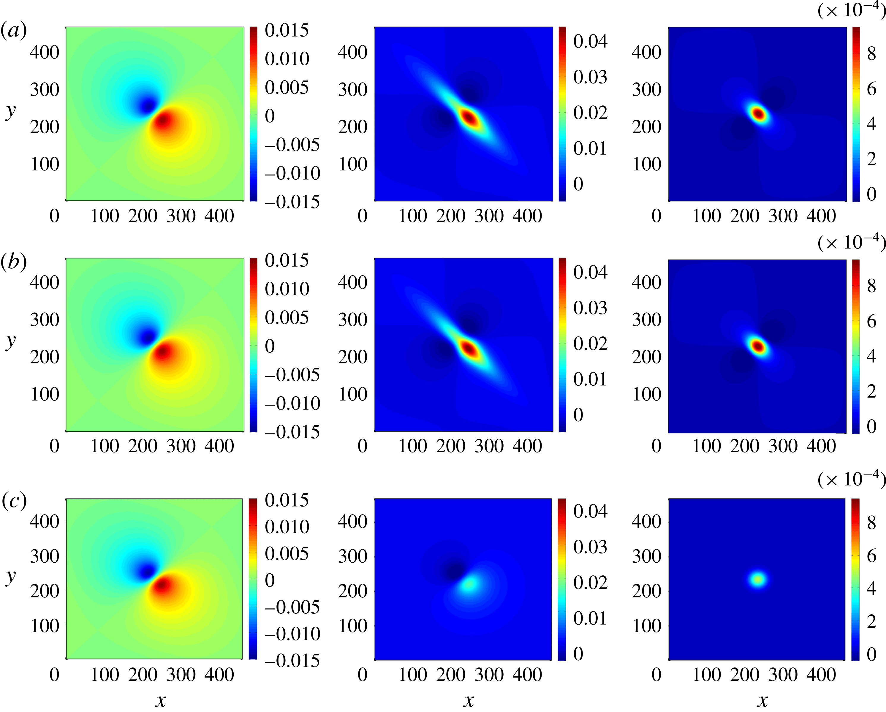
Snapshots of
 $\unicode[STIX]{x1D713}^{L}$
from wavepacket simulations. The columns from left to right correspond to the cases of weak, moderate, and strong rotation in (5.3). (a) Shows analytic results based on the co-moving equations in § 3.4, (b) is from the direct numerical simulations and (c) shows analytic results based on the steady approximation in § 3.4.

Figure 1 shows results for
 $\unicode[STIX]{x1D713}^{L}$
at a moment in the simulations when the wavepacket is in the centre of the domain. It illustrates excellent agreement between the analytic results obtained in the co-moving frame and the direct numerical simulations. On the other hand, the steady approximation is only really accurate in the non-rotating case, when all three methods reduce to the Bretherton flow. As expected from § 3.4, in the strong rotation case the steady approximation captures the monopole supported on the wavepacket footprint, but it misses the non-local part of
 $\unicode[STIX]{x1D713}^{L}$
outside the wavepacket.
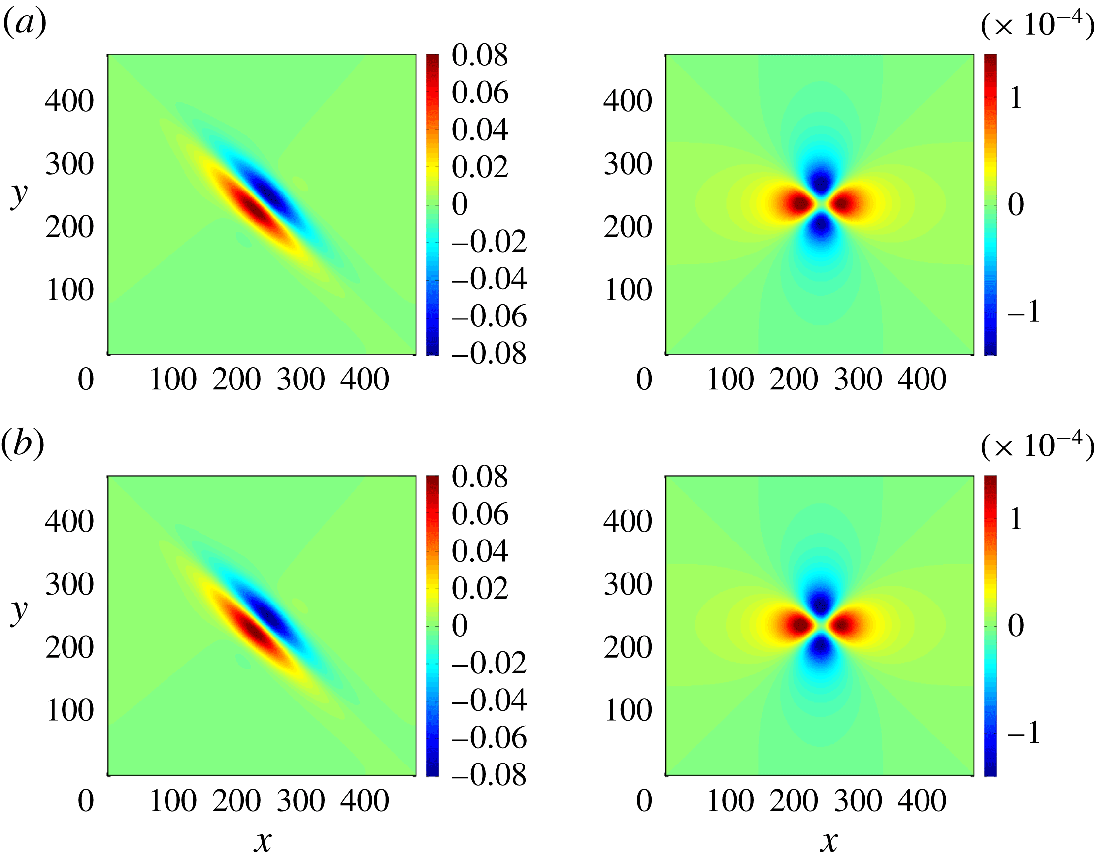
Snapshots of
 $\unicode[STIX]{x1D719}^{L}$
from wavepacket simulations with moderate rotation on the left and strong rotation on the right. (a) The analytic solution for
 $\unicode[STIX]{x1D719}^{L}$
in the co-moving frame and (b) shows results from the direct numerical simulation. No results are shown for the steady approximation, in which
 $\unicode[STIX]{x1D719}^{L}=0$
identically. Figure 3 below shows simulation results for the
 $f=0$
case, in which a steady co-moving solution for
 $\unicode[STIX]{x1D719}^{L}$
does not exist (cf. § 3.3).

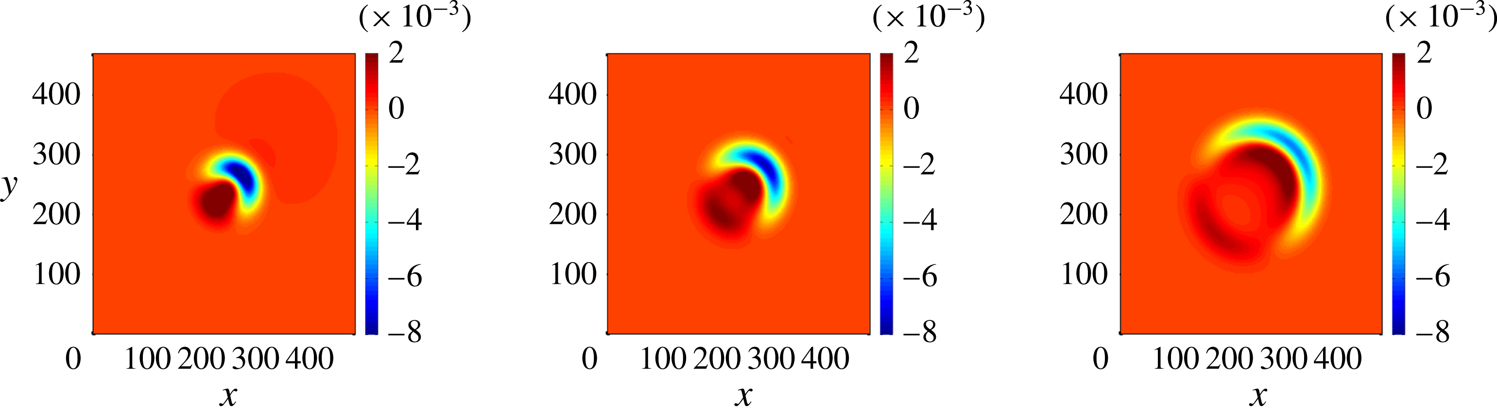
Direct wavepacket simulation time sequence of
 $\unicode[STIX]{x1D719}^{L}$
in the non-rotating case
 $f=0$
at three different times (
 $t=40,60$
and 100), illustrating that
 $\unicode[STIX]{x1D719}^{L}$
does not reach a steady state in this case.

Figure 2 shows analogous results for
 $\unicode[STIX]{x1D719}^{L}$
in the case of moderate and strong rotation, omitting the non-rotating case for which no co-moving result exists. Again, there is excellent agreement between the analytic results in the co-moving frame and the direct numerical simulations. Notably, the magnitude of
 $\unicode[STIX]{x1D719}^{L}$
is comparable to the magnitude of
 $\unicode[STIX]{x1D713}^{L}$
in these cases, so both components are needed for an accurate prediction of
 $\overline{\boldsymbol{u}}^{L}$
. Finally, in the non-rotating case a time sequence of
 $\unicode[STIX]{x1D719}^{L}$
centred at the wavepacket shown in figure 3 illustrates the growing and widening bow wave in this resonant case.
5.2 Standing wave simulations
For the standing wave field we chose the simple pattern
 ${\hat{h}}=\cos x\cos y$
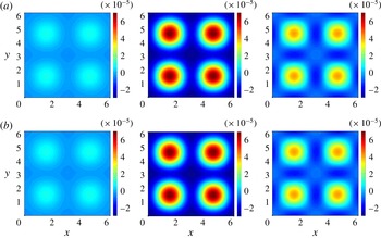
and this field together with the corresponding linear velocity fields was then used to initialize the numerical simulations. Results are presented in figure 4. As predicted by inspecting (4.8) and (4.10), the mean flow vanishes at
 $f=0$
and on increasing
 $f$
the Lagrangian flow increases in magnitude, reaches a peak, and then begins to decay. Although the strength of the mean flow varies with
 $f$
, unlike the case of a wavepacket, the spatial structure of the mean flow remains the same, at least for this very simple choice of
 ${\hat{h}}$
.
Snapshots of
 $\unicode[STIX]{x1D713}^{L}$
for standing wave case with
 ${\hat{h}}=\cos x\cos y$
. The potential
 $\unicode[STIX]{x1D719}^{L}=0$
for standing waves. Asymptotic results are in (a) and direct simulation results are in (b).
 $f=0.1,1$
and 10 from left to right.

5.3 Kinetic mean-flow energy dependence on
 $f$

We computed the dependence of the total, domain-integrated mean-flow kinetic energy on the rotation rate
 $f$
for both wavepackets and standing waves. As
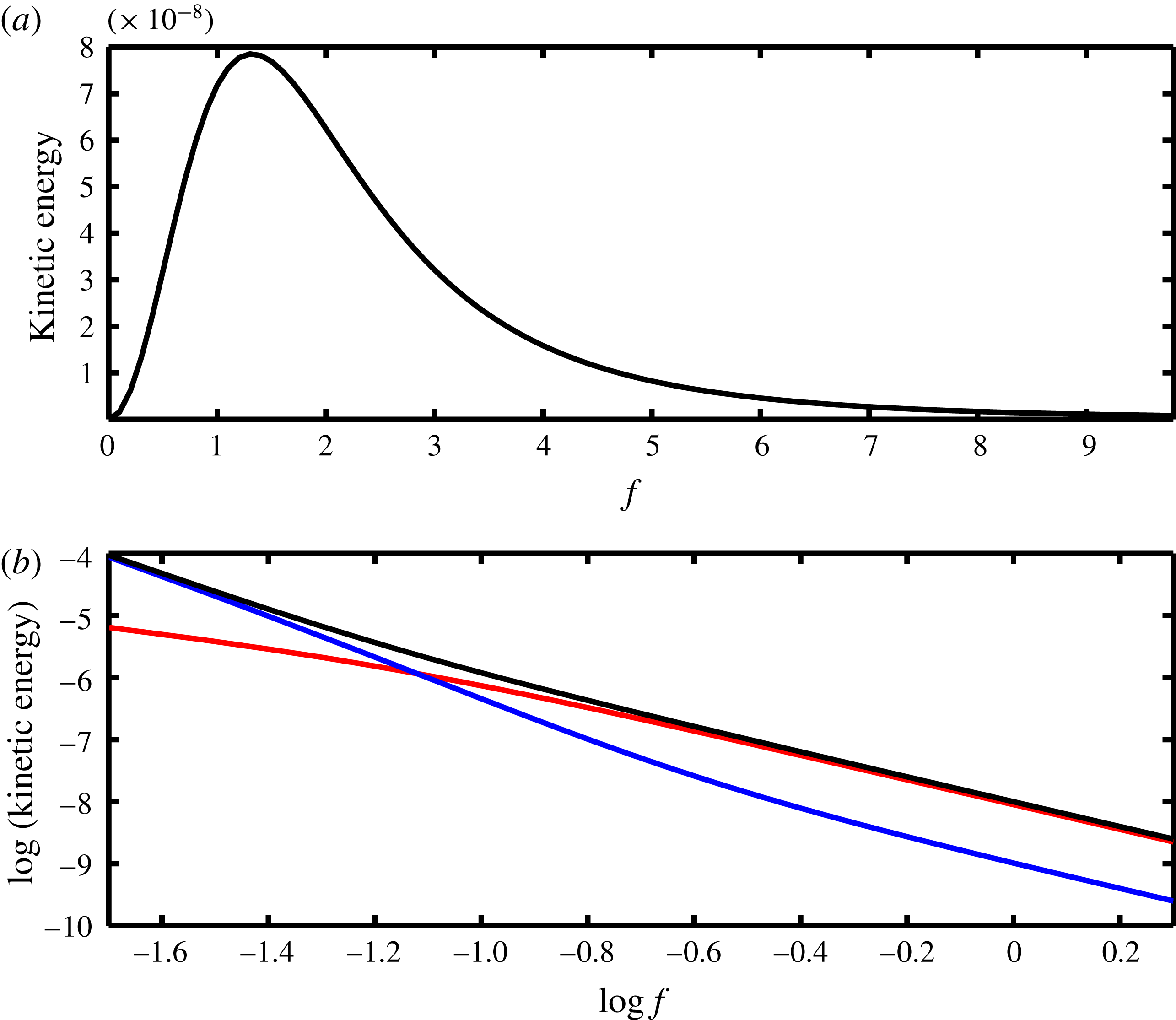
 $f$
was varied the wave amplitudes were adjusted as needed in order to keep the total energy of the wave field fixed. Results are shown in figure 5(a) corresponding to standing waves and the lower panel to wavepackets.
Domain-integrated kinetic mean-flow energy versus
 $f$
for standing wave (a) and wavepacket (b) cases. The total energy of the wave field was fixed whilst varying
 $f$
. The black curve is the total mean-flow kinetic energy and the blue and red curves indicate its divergent and rotational components, respectively. For the standing wave the divergent,
 $\unicode[STIX]{x1D719}^{L}$
-related part of the energy is identically zero and hence the black and red curves coincide. Note the logarithmic scales on the second plot.

In both cases we find that for very large
 $f$
, the mean flow is ‘choked’ and its kinetic energy decreases to zero, as noted before. However, for low
 $f$
the behaviour is markedly different in the two cases: for standing waves the mean-flow kinetic energy goes to zero also at
 $f=0$
, and hence there is an energy maximum for some intermediate value of
 $f$
, whilst for wavepackets the mean-flow kinetic energy is monotonically decreasing with
 $f$
. Furthermore, from figure 5(b), we see that at low rotation rates the potential part contributes more with negligible contribution from streamfunction part, a scenario that reverses at high rotation rates. Hence for wavepackets we observe a non-trivial cross-over of mean-flow kinetic energy from its divergent to its rotational form as
 $f$
is increased. This is not the case for standing waves, of course, for which the divergent part of
 $\overline{\boldsymbol{u}}^{L}$
is always zero.
6 Concluding remarks
We have computed the full
 $O(a^{2})$
wave-induced mean-flow response in rotating shallow water under the key assumption of uniform PV in a number of illustrative examples. As we did not assume at the outset that the mean flow had to be balanced, we were able to compute the full mean-flow response, which includes wave-like contributions to
 $\overline{\boldsymbol{u}}^{L}$
mediated by the potential
 $\unicode[STIX]{x1D719}^{L}$
. For steady waves these contributions are zero and we recovered the modified diagnostic relations between
 $\unicode[STIX]{x1D713}^{L}$
and certain wave properties that are usually associated with balanced mean flows. For unsteady wavepackets it is less obvious how to define a useful modified diagnostic relation, but this was achieved by focusing on the co-moving velocity field
 $\overline{\boldsymbol{u}}^{L}$
travelling with the wavepacket. Notably, for rotating flows this co-moving field contained comparable contributions from both
 $\unicode[STIX]{x1D713}^{L}$
and
 $\unicode[STIX]{x1D719}^{L}$
, so in this sense the concept of a modified diagnostic relation was here extended to include
 $\unicode[STIX]{x1D719}^{L}$
as well. Mutatis mutandis, we expect these shallow-water results to generalize to three-dimensional rotating Boussinesq flows, including the peculiar finding that for standing waves the mean-flow response is maximized at an intermediate value of the Coriolis parameter
 $f$
. Likewise, the extension of the present examples to weak PV perturbations would presumably lead to the usual quasi-geostrophic terms being added to the modified diagnostic relations. Of course, the nature and consequence of the long-time interactions between non-trivial PV signals and wave fields remain open questions.
We note in closing a heuristic application of our wavepacket analysis to the effective horizontal diffusion of particles in rotating shallow water. This problem was solved in Bühler & Holmes-Cerfon (Reference Bühler and Holmes-Cerfon2009) in the context of wave fields realized as small-amplitude Gaussian random fields. Alternatively, one could realize a prescribed wave power spectrum as an uncorrelated ensemble of compactly supported wavepackets, to each of which the mean-flow analysis of the present paper applies. (The phase-averaging method deployed in § 5.1 yields a smooth
 $\overline{\boldsymbol{u}}^{L}$
, but we believe that a single wavepacket experiment would produce the same irreversible particle displacements augmented by further reversible oscillations on the scale of the primary wave crests.) Specifically, any particle would then experience the time history of the co-moving velocity field
 $\overline{\boldsymbol{u}}^{L}$
due to a passing wavepacket. At
 $O(a^{2})$
, the net displacement suffered by the particle due to such a velocity field is therefore proportional to the line integral of the co-moving velocity field along a line parallel to the group velocity and intersecting the starting position of the particle. For example, these are lines at a
 $45^{\circ }$
angle in the figures in § 5.1. The net displacement therefore only depends on the distance between the original particle position and the wavepacket track. Moreover, it appears from inspection of the spatial patterns of
 $\unicode[STIX]{x1D713}^{L}$
and
 $\unicode[STIX]{x1D719}^{L}$
in figures 1 and 2 that only the rotational, streamfunction pattern makes a non-zero contribution to the net displacement of the particle, because the integral of
 $\unicode[STIX]{x1D719}^{L}$
contributions cancels along lines parallel to the group velocity whereas the integral of
 $\unicode[STIX]{x1D713}^{L}$
does not. If this heuristic argument is true it would indicate that the non-zero
 $\unicode[STIX]{x1D719}^{L}$
fields in the wavepacket case, which are comparable in magnitude to the
 $\unicode[STIX]{x1D713}^{L}$
fields, nevertheless do not lead to lasting particle displacements, and are therefore of secondary importance for transport and diffusion.
Acknowledgements
We gratefully acknowledge constructive and thought-provoking comments by the referees, which improved our paper. O.B. acknowledges financial support from the United States National Science Foundation grant DMS-1312159 and Office of Naval Research grant N00014-15-1-2355. K.S.S. and J.T. acknowledge support from the Center for Prototype Climate Modeling, a unit of the New York University Abu Dhabi Institute.
Appendix A. Error in BM98
The second term in the diagnostic relation (3.11) for the steady wavetrain response can be written as
 $$\begin{eqnarray}-\frac{f\overline{h}^{S}}{2H}=-\frac{f}{c^{2}}\frac{g\overline{h}^{S}}{2}=-\frac{f}{c^{2}}\frac{g\overline{{h^{\prime }}^{2}}}{2H}=-\frac{f}{c^{2}}\left(1-\frac{f^{2}}{\unicode[STIX]{x1D714}^{2}}\right)\frac{E}{2}.\end{eqnarray}$$
On the other hand, combining (6.6) and (7.1) from BM98 in the present shallow-water case (
 $\unicode[STIX]{x1D6FE}=2$
) yields a different term, namely
 $$\begin{eqnarray}-\frac{f}{c^{2}}\frac{1}{2}\overline{|\boldsymbol{u}^{\prime }|^{2}}=-\frac{f}{c^{2}}\left(1+\frac{f^{2}}{\unicode[STIX]{x1D714}^{2}}\right)\frac{E}{2}.\end{eqnarray}$$
Hence in the present paper the term is proportional to the potential part of the wave energy whereas in BM98 it was proportional to the kinetic part of the wave energy. Those are not equal and there is a quantitative discrepancy with BM98.
The reason for the discrepancy is a subtle error in the manipulation of the mean momentum equation in BM98. This involved using (2.5) to write
 $$\begin{eqnarray}-\overline{(\boldsymbol{u}^{\prime }\boldsymbol{\cdot }\unicode[STIX]{x1D735})\boldsymbol{u}^{\prime }}=-\frac{1}{2}\unicode[STIX]{x1D735}\overline{|\boldsymbol{u}^{\prime }|^{2}}-\overline{(\unicode[STIX]{x1D735}\times \boldsymbol{u}^{\prime })\times \boldsymbol{u}^{\prime }}=-\frac{1}{2}\unicode[STIX]{x1D735}\overline{|\boldsymbol{u}^{\prime }|^{2}}-\boldsymbol{f}\times \frac{\overline{h^{\prime }\boldsymbol{u}^{\prime }}}{H}\end{eqnarray}$$
and then replacing the last term with
 $-\boldsymbol{f}\times \overline{\boldsymbol{u}}^{S}$
based on the plane-wave relations (3.4). However, this introduces an
 $O(\unicode[STIX]{x1D707}a^{2})$
error term, as the plane-wave relations are not exact for a slowly varying wavetrain. The omitted error term is
 $$\begin{eqnarray}-\boldsymbol{f}\times \left(\frac{\overline{h^{\prime }\boldsymbol{u}^{\prime }}}{H}-\overline{\boldsymbol{u}}^{S}\right)=\boldsymbol{f}\times \left(\overline{(\unicode[STIX]{x1D709}_{j}^{\prime }\boldsymbol{u}^{\prime })}_{,j}\right)=-\unicode[STIX]{x1D735}f\overline{\unicode[STIX]{x1D709}^{\prime }v^{\prime }}=-\frac{1}{2}\unicode[STIX]{x1D735}\overline{\boldsymbol{u}^{\prime }\boldsymbol{\cdot }\boldsymbol{f}\times \unicode[STIX]{x1D743}^{\prime }}.\end{eqnarray}$$
This uses
 $\overline{\unicode[STIX]{x1D709}^{\prime }u^{\prime }}=\overline{\unicode[STIX]{x1D702}^{\prime }v^{\prime }}=0$
and
 $\overline{\unicode[STIX]{x1D702}^{\prime }u^{\prime }}=-\overline{\unicode[STIX]{x1D709}^{\prime }v^{\prime }}$
in the present situation of a steady wavetrain. Combining this with the first term in (A 3) and applying the steady virial theorem (2.12) finally yields
 $$\begin{eqnarray}-\frac{1}{2}\unicode[STIX]{x1D735}\left(\overline{|\boldsymbol{u}^{\prime }|^{2}}+\overline{\boldsymbol{u}^{\prime }\boldsymbol{\cdot }\boldsymbol{f}\times \unicode[STIX]{x1D743}^{\prime }}\right)=-\frac{g\overline{h}^{S}}{2},\end{eqnarray}$$
which eventually recovers the correct term, as in the present paper.