1. Introduction
In many natural and industrial systems, thermal convection occurs in fluid layers heated from below and with free and evaporative upper surfaces, where the interplay between heat and mass transfer governs the system dynamics. Moreover, these systems have usually large aspect ratios
 $\varGamma$
, whereby their width
 $L$
is much larger than their height
 $h$
. Examples include cooling ponds in power plants (Brewster Reference Brewster2018), ocean–atmosphere interactions (Mangarella et al. Reference Mangarella, Chambers, Street and Hsu1973; Falor et al. Reference Falor, Gayen, Sengupta and Ivey2023), convection in sun-like stars (Schumacher & Sreenivasan Reference Schumacher and Sreenivasan2020; Pandey, Schumacher & Sreenivasan Reference Pandey, Schumacher and Sreenivasan2021) and cryogenic or planetary processes (Morison, Labrosse & Choblet Reference Morison, Labrosse and Choblet2021). In such cases, the upper boundary condition is not rigid nor perfectly conductive as in classical Rayleigh–Bénard convection, but is instead a deformable, evaporating interface exposed to ambient air. This system can therefore be regarded as a combination of an evaporative cooling set-up (Spangenberg & Rowland Reference Spangenberg and Rowland1961; Katsaros et al. Reference Katsaros, Liu, Businger and Tillman1977; Doumenc et al. Reference Doumenc, Boeck, Guerrier and Rossi2010; Pushtaev et al. Reference Pushtaev, Vinnichenko, Plaksina and Uvarov2021) and a classical Rayleigh–Bénard set-up with a free upper surface, where the heat exchange strongly depends on the physical phenomena at play above the interface (figure 1). The resulting convective behaviour of the liquid is partly controlled by the coupling between evaporation, latent heat flux, radiative transfer from the interface and natural convection in the gas (air + water vapour) phase. As will be shown below, each of these phenomena has already been studied, but a detailed understanding of their interactions in the case of convection–evaporation is still lacking. In particular, two key questions remain: (i) how the phase change is going to affect/control the convective patterns and the heat transfer in the liquid layer, and (ii) to which extent the framework of classical Rayleigh–Bénard convection remains useful to describe the dynamics of the liquid layer.
1.1. Classical Rayleigh–Bénard convection (RBC)
Rayleigh–Bénard convection involves a layer of fluid heated from below and cooled from above through two perfectly conducting horizontal planes. It has been extensively studied as a canonical example of a pattern-forming instability (see Manneville Reference Manneville2006), exhibiting a route to chaos, turbulence and its ‘ultimate’ regime (Kraichnan Reference Kraichnan1962; Grossmann & Lohse Reference Grossmann and Lohse2011; Roche Reference Roche2020; Lohse & Shishkina Reference Lohse and Shishkina2024). Buoyancy drives the convective instabilities when the ratio between the diffusive time scale and the convective time scale, represented by the Rayleigh number
 $ \textit{Ra} = ({g\alpha \Delta T h^3}/{\kappa \nu })$
(where
 $g$
is the acceleration due to gravity,
 $\alpha$
is the thermal expansion coefficient,
 $\kappa$
is the thermal diffusivity of the fluid,
 $\nu$
is the kinematic viscosity of the fluid and
 $ \Delta T$
is the difference of temperature applied across the layer) is above a critical threshold (
 $ \textit{Ra}_c=1708$
for rigid boundaries and
 $ \textit{Ra}_c=657$
for free boundaries; Chandrasekhar Reference Chandrasekhar1961). At high
 $ \textit{Ra} $
, convective instabilities develop as plumes from the cold and hot thermal boundary layers, which should generate a heat transfer scaling as
 $ \textit{Nu} \sim \textit{Ra}^{1/3}$
(e.g. Howard Reference Howard1966), where the Nusselt number
 $Nu$
is the surface heat flux normalized by the conductive heat flux through the layer. The other parameter needed to fully describe the dynamics is the Prandtl number
 $ \textit{Pr}= ({\nu }/{\kappa })$
, which represents the ratio between the two diffusive mechanisms (diffusion of heat and diffusion of momentum) involved in the system. In low Prandtl number fluids such as water or air, a large-scale circulation (LSC) is observed in addition to the classical thermal boundary layers instabilities. This is due to the interaction between the plumes (e.g. Krishnamurti & Howard Reference Krishnamurti and Howard1981; Brown & Ahlers Reference Brown and Ahlers2008; Xi & Xia Reference Xi and Xia2008). The LSC is probably responsible for the lower exponent (0.28–0.31) in the Nu–Ra scaling observed at least up to
 $ \textit{Ra} \sim 10^{12}$
(e.g. see Chillà & Schumacher Reference Chillà and Schumacher2012 for a review). First observed spanning the whole tank in low aspect ratios systems, the LSC in fact takes the form of several turbulent superstructures when
 $\varGamma \gt 10{-}20$
(Bailon-Cuba, Emran & Schumacher Reference Bailon-Cuba, Emran and Schumacher2010; Pandey, Scheel & Schumacher Reference Pandey, Scheel and Schumacher2018; Blass et al. Reference Blass, Verzicco, Lohse, Stevens and Krug2021; Moller Reference Moller2022; Käufer et al. Reference Käufer, Vieweg, Schumacher and Cierpka2023). Changes in patterns are also associated with changes in small-scale statistical properties (e.g. Lohse & Xia Reference Lohse and Xia2010), in the large-scale flow velocity and in heat transfer (e.g. Ahlers, Grossmann & Lohse Reference Ahlers, Grossmann and Lohse2009; Chillà & Schumacher Reference Chillà and Schumacher2012), that mainly derive from the nature of the boundary layers and their interactions (e.g. Grossmann & Lohse Reference Grossmann and Lohse2000, Reference Grossmann and Lohse2004, Reference Grossmann and Lohse2011; Roche Reference Roche2020, Lohse & Shishkina Reference Lohse and Shishkina2024).
Schematic representation of the convective patterns and the different heat-flux contributions involved during the convection–evaporation of water.

The nature of the boundary conditions at the horizontal surfaces are also important (e.g. Chillà & Schumacher Reference Chillà and Schumacher2012). For instance, replacing one rigid by one free surface decreases the critical Rayleigh number down to
 $ \textit{Ra}_c=1101$
(Chandrasekhar Reference Chandrasekhar1961). And replacing perfectly conductive boundaries by plates with finite conductivity decreases
 $ \textit{Ra}_c$
, increases the size of the convective cells and modifies the distribution of temperature (Hurle et al. Reference Hurle, Jakeman, Pike and Sutton1967; Riahi Reference Riahi1985; Falsaperla & Giacobbe Reference Falsaperla and Giacobbe2012; Käufer et al. Reference Käufer, Vieweg, Schumacher and Cierpka2023).
1.2. Evaporative cooling and penetrative convection
In this case, a layer of initially isothermal fluid is cooled through evaporation at its upper surface, and therefore release of latent heat. This surface cooling generates a thermal boundary layer that becomes unstable (Howard Reference Howard1966). Experimental observations showed that cold material accumulated along lines on the surface before plunging downwards (Spangenberg & Rowland Reference Spangenberg and Rowland1961). As there is no heating from below, only cold downwelling plumes exist and there should be no LSC in the liquid layer. Indeed, Katsaros et al. (Reference Katsaros, Liu, Businger and Tillman1977) measured
 $ \textit{Nu}=0.156 \textit{Ra}^{0.33}$
across the liquid cold thermal boundary layer. On the air side above the interface, Bower & Saylor (Reference Bower and Saylor2009) showed that it was important to consider the release by evaporation of water vapour (which is lighter than air) in the buoyancy budget. Based on laboratory measurements, they established a scaling law between the adimensioned evaporation rate (characterised by the Sherwood number
 $ \textit{Sh}$
) and the Rayleigh number (based on the total buoyancy) in the convecting air layer.
1.3. Convection–evaporation
On the other hand, in the case of convection–evaporation when the layer is also heated from below, the lower hot and upper cold boundary layers are both active, and a LSC is expected. Poós & Varju (Reference Poós and Varju2024) recently reviewed the different conditions (such as the existence of wind in the air layer above the interface) under which convection and evaporation can be coupled, and the associated studies. We shall restrict our investigation to the case with no wind forcing in the air, i.e. their ‘N-S-T’ category (natural convection in the gas, constant gas conditions but variable liquid conditions), where only few results exist. Zhang, Chong & Xia (Reference Zhang, Chong and Xia2019) studied experimentally and numerically a two-layer system heated from below where the bottom liquid layer convects and evaporates, producing above the interface a convective layer of moist air that can condensate at the upper cold surface. They were able to measure the moisture transfer rates and proposed scaling laws for the heat and mass transfers in the evaporating-condensing moist air layer, using a generalised buoyancy (thermal and compositional contributions of the water vapour) approach. Hay & Papalexandris (Reference Hay and Papalexandris2020) studied numerically the convective patterns and heat transfer in a cubic layer of water heated from below as a function of
 $ \textit{Ra} $
, using a proxy to describe the evaporating free surface: they prescribed on the top water surface a free-slip condition and a constant heat flux. The latter is due to the latent heat release of evaporation and to convection in the dry air, where the transfer of water vapour is not considered. They observed the establishment of a circulation over the whole box and reported a Nu–Ra scaling law of a form similar to RBC. Another proxy could be the use of a thermal conductivity that decreases strongly with temperature. In this case, the numerical simulations of Pandey et al. (Reference Pandey, Schumacher and Sreenivasan2021) run at
 $\varGamma = 16$
show the existence of several turbulent superstructures. Very recently, Carlier & Papalexandris (Reference Carlier and Papalexandris2024) solved the fully coupled equations in both water and air layers, when there is no condensation in the air layer. They described in detail the dynamics of the two layers for
 $\varGamma =2$
and
 $ \textit{Ra} = 5.8{-}6.85\times 10^5$
.
Our aim is therefore to characterise the contributions of convection, evaporation and radiation on the convective patterns and heat and mass transfers for an extended range of
 $ \textit{Ra} $
(up to 4.10
 $^7$
) and
 $\varGamma$
(5–30). To be able to disentangle the influence of the different physical phenomena at play, three sets of experiments have been carried out: convection–evaporation, evaporation without heating from below and convection without evaporation. High-resolution thermal Infrared (IR) imaging of the surface, and mass transfer measurements are used to study the water–air coupled system as a function of ambient conditions (temperature, humidity) and bottom heating, liquid height and tank size. Section 2 presents the experimental procedure and the dimensionless numbers needed to describe the dynamics. Section 3 describes the time evolution of a typical experiment and the different scales of motion encountered. Section 4 discusses the scaling laws derived from the experiments for the typical spacing of the different scales of motion, the heat and mass transfers and the water surface mean temperature.
2. Laboratory experiments
2.1. Experimental set-up
An Altuglas tank is filled with distilled and deionised water and is heated from below by a copper plate maintained at constant and uniform temperature (figure 2). The upper surface is free and allows the water to evaporate into a much larger room, considered as an infinite medium, maintained at ambient temperature (
 $T_{\textit{amb}} \approx {20}\,^\circ\textrm {C}$
) and at atmospheric pressure. Two different tanks were used of square base
 $20\, \mathrm{cm} \times 20\,\mathrm{cm}$
and
 $30\, \mathrm{cm} \times 30\,\mathrm{cm}$
. To avoid capillary effects near the walls, they were sprayed with a thin hydrophobic layer before each experiment. The bottom temperature is recorded with two (type-K) thermocouples embedded within the copper plate, and the mid-tank water temperature with a platinum probe linked to a MKT50 (Anton Paar), with a precision
 ${\pm} \lt{0.05}\,^\circ\mathrm{C}$
.
Experimental set-up.

Ambient temperature and humidity rate are recorded with a Dostmann Electronic P755-Log, with precisions
 $\pm {0.2}\,^\circ\textrm {C}$
and
 $\pm 1.5 \,\%$
, respectively. The mean air velocity was measured with a KIMO SOM 900 omnidirectional probe. Far from the surface, the average velocity was measured at
 ${0.04\pm (0.05) }\,\textrm m\,\rm s^-{^1}$
, with a maximum instantaneous velocity of
 ${0.26\pm (0.01)}\,\textrm m\,\rm s^-{^1}$
recorded. However, no evidence of background air velocity was found in the empty tank. As the air layer above the surface of the water layer is protected from the room air flux by the tank sidewalls (always at least 5 cm higher than the water surface), the air layer above the water layer is only subject to natural convection, without any forced convection contribution from the room.
The experimental tank is placed on a balance (FC64EDE-S from Sartorius, precise at
 $\pm {1}\,\textrm {g}$
) that records the mass of water
 $m(t)$
remaining in the tank at each time
 $t$
. From it are deduced the evaporation rate
 $\textrm{d}m/\textrm{d}t$
and the height of water
 $h(t)$
 \begin{align} h(t)=\frac {m(t)}{\rho (T_{\textit{surf}}) L^2}, \end{align}
where
 $\rho$
is the density of water.
The temperature distribution at the water surface is recorded by a FLIR A655sc thermal long wave infrared range (LWIR) camera with a focal length
 $f={26.6}\,{\mathrm{mm}}$
(
 $f={13.1}\,{\mathrm{mm}}$
for the largest tank) IR lens placed at
 $D=70\,\mathrm{cm}$
(
 $D=55\,\mathrm{cm}$
respectively) above the tank. The spatial resolution of the camera in these conditions is
 ${0.4}\,\textrm {mm} ({0.7}\,\textrm {mm})$
. The emissivity of water is set at
 $\epsilon =0.95$
and is required to convert the radiance data recorded by the camera into a temperature scale. In the LWIR (i.e.
 $\lambda \in [{7.5 }\,\unicode{x03BC} \textrm {m},{14}\,\unicode{x03BC} \textrm {m}]$
), water has a high absorption coefficient (superior to
 ${250}\,\textrm {cm}^{-1}$
, Bayly, Kartha & Stevens (Reference Bayly, Kartha and Stevens1963)), and the IR signal is only sensitive to the upper
 ${30}\,\unicode{x03BC} \textrm {m}$
of the water layer (Plyler & Acquista Reference Plyler and Acquista1954).
The absorption coefficient of water vapour in the LWIR and in the range of temperatures and humidity rates used in this work is between
 $1 \times 10^{-6}\,\textrm {cm}^{-1}$
and
 $3 \times 10^{-6}\,\textrm {cm}^{-1}$
(Thomas Reference Thomas1987), which is much lower than that of liquid water. The contribution of water vapour to the IR signal is thus negligible compared with that of the liquid water. As a consequence, the IR signal corresponds to the temperature of the surface.
The acquisition frequency ranged between 25 images per seconds, and one image every 10 minutes. The latter is much larger than the typical free-fall time of each experiment (
 $\approx {2}\,\textrm {s}$
); it was used to study the long-term evolution of the experiments. The higher acquisition frequencies allow us to follow the dynamic of individual plumes. Moreover, the camera shutter speed is high enough (greater than 25 Hz) to avoid blurry images due to the motions of thermal features at the surface.
All temperature measurements were calibrated beforehand to eliminate any potential mismatch between the measurements. The camera was calibrated by comparing the spatially averaged temperature of a black plate with the value measured by the various thermocouples and platinum probes. After calibration of the set-up, the precision of the IR camera is 30 mK.
Two geometrical effects were corrected in the IR images. (i) The inclination of the camera is removed by using the corners of the tank as references and applying a projection algorithm. (ii) As water evaporates, the distance between the camera and the surface increases and features on the surface appear smaller. The ratio of the apparent length scale
 $L_{\textit{ap}}$
and the true length scale
 $L$
is given by
 \begin{align} \frac {L_{\textit{ap}}(t)}{L}=\frac {D-h_0}{D-h(t)}, \end{align}
where
 $h_0$
is the initial height of the fluid and
 $D$
the distance between the camera and the bottom plate of the tank. Finally, a
 $5\times 5$
pixel Wiener filter is applied to each image to remove the noise of the IR camera. This
 $5\times 5$
pixel kernel corresponds to a 3 mm
 $\times$
3 mm window for the 20 cm
 $\times$
20 cm tank and a 4 mm
 $\times$
4 mm for the 30 cm
 $\times$
30 cm tank. Therefore, the filtering window remains much smaller than the smallest convective features (figures 3, 4, 8 and 9).
Once the IR images have been corrected, we denote by
 $T_{\textit{IR}}$
the temperature of the surface as measured by the IR camera, and the horizontally averaged temperature of the surface is
 $T_{\textit{surf}} = \langle T_{\textit{IR}} \rangle _{x,\,y}$
.
2.2. Dimensionless numbers
Our system can be seen as two superimposed convecting fluid layers, of water and air/vapour (figure 1). The properties of the liquid will be denoted using the subscript
 $_L$
, and those of the humid air will be denoted with the subscript
 $_{V}$
. The properties relative to the dry air will be denoted using the subscript
 $_G$
. The properties of water and air vary with temperature (see Appendix A). For water, their values are taken at
 $T_{\textit{surf}}$
because the platinum probe (figure 2) shows that the temperature in the water bulk remains close to the temperature of the surface. The properties of the air are taken at ambient temperature and humidity rate (figure 2).
2.2.1. Water layer
For water layer depths greater than 10 mm, as is mostly the case here, buoyancy forces are more effective than surface tension forces to generate instabilities from the upper water surface (Pearson Reference Pearson1958; Katsaros et al. Reference Katsaros, Liu, Businger and Tillman1977; Doumenc et al. Reference Doumenc, Boeck, Guerrier and Rossi2010). In addition, thermal Bénard–Marangoni convection has proven very hard to observe in aqueous systems because of surface contamination (Berg, Boudart & Acrivos Reference Berg, Boudart and Acrivos1966; Doumenc et al. Reference Doumenc, Boeck, Guerrier and Rossi2010). In our experiments, the free surface remains exposed to the environment for long times (up to one week), so surface contamination certainly occurs during this time and prevents Bénard–Marangoni convection from settling. This is why we adopt the framework of RBC in our analysis, without considering Bénard–Marangoni effects. The dynamics is then described by three dimensionless numbers:
-
(i) the aspect ratio of the layer of water compares the length of the tank with the remaining height of water. In the evaporative experiments, this ratio increases along time
(2.3) \begin{align} \varGamma (t) = \frac {L}{h(t)}; \end{align}
-
(ii) the Rayleigh number compares the characteristic time of convection with the characteristic time of heat and momentum diffusion
(2.4)where
\begin{align} \textit{Ra}(t) = \frac {g\alpha _L(T_{\textit{surf}})}{\kappa _L(T_{\textit{surf}}) \nu _L(T_{\textit{surf}}) } (T_{\textit{bot}}-T_{\textit{surf}}) h(t)^3, \end{align}
$g$
is the gravity acceleration,
$\alpha$
is the thermal expansion,
$\kappa$
is the thermal diffusivity and
$\nu$
the kinematic viscosity.
-
(iii) the Prandtl number is defined as the ratio of momentum diffusivity to thermal diffusivity
(2.5)The Prandtl number remains approximately constant during all the experiments performed, with a value between 4 and 6.
\begin{align} \textit{Pr}_L = \frac {\nu _L(T_{\textit{surf}})}{\kappa _L(T_{\textit{surf}})} . \end{align}


2.2.2. Humid air layer
The buoyancy of the material just above the interface has two components: one due to the temperature gradient (the interface being hotter than the ambient temperature of the room), and one due to the gradient of partial pressure of water (the air is richer in water close to the evaporating surface). Convection above the water surface is therefore driven by two components, and constitutes an end-member case of double-diffusive convection (e.g. Yang, Verzicco & Lohse Reference Yang, Verzicco and Lohse2018; Zhang et al. Reference Zhang, Chong and Xia2019).
-
(i) The Prandtl number in the air is
(2.6)
\begin{align} \textit{Pr}_V = \frac {\nu _V(T_{\textit{amb}})}{\kappa _V(T_{\textit{amb}})} \approx 0.7. \end{align}
-
(ii) In addition, the Schmidt number compares the momentum diffusivity
$\nu _V$
with the mass diffusivity
$D_V$
(2.7)Note that the two numbers are very close, so that the Lewis Number
\begin{align} Sc_V = \frac {\nu _V(T_{\textit{amb}})}{D_{V}(T_{\textit{amb}})} \approx 0.6. \end{align}
$ Le= \kappa _V / D_V \approx 0.9$
is close to 1: heat and water vapour diffuse at approximately the same velocity in dry air.
-
(iii) Far from the water surface, we directly measure the humidity rate in the air, which compares the partial pressure of water
$P_{{\rm H_2O},amb}$
in the room with the saturation vapour pressure at ambient temperature
$P_{\textit{sat}}(T_{\textit{amb}})$
(2.8)Note that, at the evaporating surface,
\begin{align} \textit{HR} = \frac {P_{{\rm H_2O},amb}}{P_{\textit{sat}}(T_{\textit{amb}})}. \end{align}
$\textit{HR}=1$
.


The Grashof number (Zhang et al. Reference Zhang, Chong and Xia2019) compares the total buoyancy with the viscous forces in the air
 \begin{align} Gr=\frac {g \Delta \rho _V h_{G}^3}{\rho _V(T_{\textit{amb}})\nu _V(T_{\textit{amb}})^2} ,\end{align}
where
 $\nu _V$
is the kinematic viscosity of the air and
 $\Delta \rho _V$
the density difference given by
 \begin{align} \Delta \rho _V = \frac {M_V}{R}\left [\frac {P_{\textit{sat}}(T_{\textit{surf}})}{T_{\textit{surf}}+273.15}-HR\frac {P_{\textit{sat}}(T_{\textit{amb}})}{T_{\textit{amb}}+273.15}\right ]\!, \end{align}
where
 $M_V$
is the molar mass of water.
Moreover,
 $h_G$
is a characteristic length of convection in the air. As we are in a semi-infinite layer, the only characteristic length scale available to describe convection in the air is the width of the tank
 $L$
, so we take
 $h_G=L$
. We use Tetens’ formula (Tetens Reference Tetens1930, Monteith & Unsworth Reference Monteith and Unsworth2013) to determine
 $P_{\textit{sat}}(T)$
 \begin{align} P_{\textit{sat}}(T)=P_{\textit{sat}}(T = {0}\,^\circ \textrm {C})\exp \left (\frac {a T}{T+b}\right )\!, \end{align}
where
 $T$
is expressed in
 $^\circ \textrm {C}$
,
 $P_{\textit{sat}}(T = {0}\,^\circ \textrm {C}) = {0.61078\times 10^3}\,\textrm {Pa}$
,
 $a = {17.2693882}\,^\circ \textrm {C}^{-1}$
and
 $b = {237.3}\,^\circ \textrm {C}$
.
The Grashof number is linked to the Rayleigh and Prandtl numbers through the relation
 $ \textit{Ra}=Gr \textit{Pr}$
, which is true regardless of the fluid considered. In order to make a clear distinction between convection occurring in the air layer and convection occurring in the water layer, we will describe the convection in the air in terms of Grashof number and the convection in the water layer in terms of Rayleigh number.
2.2.3. At the interface
Compared with the case of RBC in two superimposed layers, two extra processes are occurring at the interface. First, the water evaporation generates latent heat release, which is characterised by the Stefan number
 \begin{align} St = \frac {L_{v\textit{ap}}}{C_{p,L} (T_{\textit{bot}}-T_{\textit{amb}})}, \end{align}
where
 $L_{v\textit{ap}}$
is the latent heat of vaporisation of water and
 $C_{p,L}$
is the specific heat capacity of water. Values of
 $St \gt 1$
as encountered here means that this contribution will be important for the energy budget at the interface. Second, the interface generates black body radiation in the air, which can be described by the radiative Biot number
 \begin{align} \textit{Bi}_R = \frac {\sigma \epsilon T_{\textit{amb}}^3 L}{k_{\textit{air}}}, \end{align}
where
 $k_{\textit{air}}$
is the thermal conductivity of air, and
 $\sigma = {5.670 \times 10^{-8}}\,{\textrm {Wm}}^{-2}\,\textrm {K}^{-4}$
is Stefan’s constant. Given the low thermal conductivity of air, we shall see in § 4 that this radiative contribution cannot be neglected in the energy budget of the interface for the case without evaporation.
2.3. List of experiments
For each experiment, the tank is initially filled with a given height of water
 $h_0$
and the heating is switched on at time
 $t=0$
. Then the evolution of the system is recorded through time, generally until complete evaporation of the water. This means that the duration of an experiment ranges between one day and two weeks.
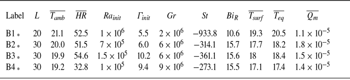
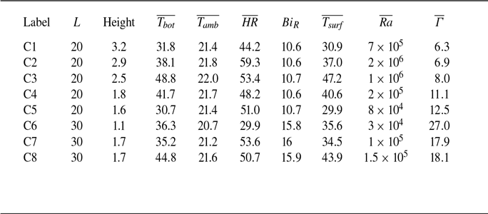
Three sets of experiments were carried out to identify the relative contributions of evaporation and RBC to the dynamics (patterns, heat and mass transfers) of the water layer. The first set (table 1) concerns the experiments of evaporation while the tank bottom boundary is heated at a constant temperature. In the second set (table 2), evaporation is occurring without heating from below. This is a case of penetrative convection only (cf. Katsaros et al. Reference Katsaros, Liu, Businger and Tillman1977). In the third set of experiments (table 3), the tank is heated from below at constant temperature but evaporation is shut down by adding a
 ${50}\,\unicode{x03BC} \textrm {m}$
thick film of polypropylene to the surface of the water. This film is transparent to IR and therefore still allows access to the interface temperature distribution.
Experiments with evaporation. Temperatures are in
 $^\circ \textrm {C}$
,
 $\textit{HR}$
is in %,
 $L$
is in cm and
 $\overline {Q_{m}}$
in
 $\mathrm{kg\, s^{-1}\,m^{-2}}$
.
 $\dagger$
: additional experiment with a frame rate of 25 images per second. A movie of experiment A10 is available in the supplementary material. When an experiment label is accompanied by a coloured dot, the same colour will represent this experiment in all the following figures. The colours range from blueish cold colours for the experiments with the lower
 $T_{\textit{bot}}$
to reddish colours for the experiments with the higher
 $T_{\textit{bot}}$
. We gave the same colour to experiments which have the same
 $T_{\textit{bot}} \pm {1}\,^\circ \textrm {C}$
.

Experiments without heating. Here,
 $T_{\textit{eq}}$
corresponds to the temperature of the lower copper plate. This plate has high thermal conductivity, and is placed between the water layer and a thermal insulator. Thus, its temperature at equilibrium is close to the bulk temperature of water. The temperature difference in
 $ \textit{Ra}_{\textit{init}}$
is
 $T_{\textit{eq}} - T_{\textit{surf}}$
.

Experiments without evaporation.

3. Time evolution of an experiment
3.1. Evaporation and heating from below
Compared with RBC, this configuration changes the water top boundary condition for a free surface and an open thermal boundary where neither the temperature nor the heat-flux distributions are constant (Katsaros et al. Reference Katsaros, Liu, Businger and Tillman1977).
Figure 3 shows the evolution of the evaporating water layer during experiment A1 (table 1). Despite the strong decrease of the Rayleigh number (due to the decrease in water depth), the temperatures and evaporation rate remain fairly constant throughout the experiment (figure 3 B). The variations around the mean recorded in the mass flux (figure 3 Bd) are anticorrelated with the humidity (figure 3 Bc).
Experiment A1 (table 1). A: Temperature of the surface at different times during an experiment. (a)
 $t = {83.3}\,\textrm {h}$
,
 $ \textit{Ra} = 1.6\times 10^6$
; (b)
 $t = {133.3}\,\textrm {h}$
,
 $ \textit{Ra} =4.7 \times 10^5$
; (c)
 $t = {166.7}\,\textrm {h}$
,
 $ \textit{Ra} = 1.7\times 10^5$
; (d)
 $t = {183.3}\,\textrm {h}$
,
 $ \textit{Ra} = 7.6\times 10^4$
; (e)
 $t = {191.6}\,\textrm {h}$
,
 $ \textit{Ra} = 5.9\times 10^4$
; (f)
 $t = {200.0}\,\textrm {h}$
,
 $ \textit{Ra} = 3.6\times 10^4$
; (g)
 $t = {208.3}\,\textrm {h}$
,
 $ \textit{Ra} = 1.9 \times 10^4$
; (h)
 $t = {216.7}\,\textrm {h}$
,
 $ \textit{Ra} = 9.4\times 10^3$
; (i)
 $t = {225.0}\,\textrm {h}$
,
 $ \textit{Ra} =4.5 \times 10^3$
; (j)
 $t = {233.3}\,\textrm {h}$
,
 $ \textit{Ra} =1.4 \times 10^3$
. The black square represents the size of the Wiener filter applied before performing the Fourier transform of the images. B: (a) Height of fluid, (b) ambient temperature (green), mean surface temperature (blue) and lower plate temperature (orange), (c) humidity rate, (d) evaporation mass flux and (e) Rayleigh number as a function of time. Here,
 $ \textit{Ra} $
evolves as
 $t^{-1/3}$
. The vertical black lines indicate the images (a) to (j).

3.1.1. Phenomenology
The temperature distribution at the surface (figure 3 A) presents a clear evolution as the Rayleigh number and water depth decrease:
-
- At the beginning of the experiment (
$ 4.10^5 \leqslant \textit{Ra} \leqslant 4.10^7$
), three types of features are distinguishable to the naked eye: (i) blue cold lines, (ii) red hot roundish patches, (iii) a large-scale distribution of the cold and hot heterogeneities in two broad zones along the diagonal of the tank (figure 3
Aa). The latter is also clearly seen on a time-averaged image of the temperature (figure 4), while (i) and (ii) disappear due to their strong time dependence. (i) Can therefore be interpreted as cold sheet-like plumes developing from the instability of the evaporating cold upper thermal boundary layer, while (ii) are the signatures of hot three-dimensional plumes coming from the lower hot boundary layer and impinging under the surface. ‘Sheet-like’ (or ‘line’) plumes developing from boundary layers have already been observed in purely evaporative convection (Spangenberg & Rowland Reference Spangenberg and Rowland1961), in solutal convection (Puthenveettil & Arakeri Reference Puthenveettil and Arakeri2005) and in classical RBC (Theerthan & Arakeri Reference Theerthan and Arakeri1998; Shishkina & Wagner Reference Shishkina and Wagner2008; Zhou & Xia Reference Zhou and Xia2010; Puthenveettil et al. Reference Puthenveettil, Gunasegarane, Agrawal, Schmeling, Bosbach and Arakeri2011; Shevkar et al. Reference Shevkar, Mohanan, Koothur, Mathur and Puthenveettil2022), while three-dimensional plumes develop from the junction of the lines (Houseman Reference Houseman1990; Xi, Lam & Xia Reference Xi, Lam and Xia2004). It is therefore expected that, here, the top surface records cold lines (in the thermal boundary layer) and hot roundish plumes (which have broken from their original boundary layer). Moreover, the large-scale distribution of temperature (figures 3
A and 4) is the signature of the LSC of the plumes in the tank (Krishnamurti & Howard Reference Krishnamurti and Howard1981). Despite the LSC, hot water plumes have been reported to reach the top surface for
$ \textit{Ra} $
at least up to
$10^8$
(Malkus Reference Malkus1954). -
- As evaporation proceeds, the water depth diminishes, so that
$ \textit{Ra} $
diminishes but the aspect ratio of the water layer increases. Although the thermal plumes features (i) and (ii) are still observed, figure 3(Ac–g) now show several larger-scale cells superimposed on the plumes. Similar observations have been reported in classical RBC when the aspect ratio is greater than 10–20, in both experiments (Moller Reference Moller2022) and Direct Numerical Simulations (DNS) (Bailon-Cuba et al. Reference Bailon-Cuba, Emran and Schumacher2010; Pandey et al. Reference Pandey, Scheel and Schumacher2018; Blass et al. Reference Blass, Verzicco, Lohse, Stevens and Krug2021; Käufer et al. Reference Käufer, Vieweg, Schumacher and Cierpka2023). Moreover, numerical simulations with a temperature-dependent thermal conductivity also display this superposition of thin cold patterns and larger roundish hot patches (Pandey et al. Reference Pandey, Schumacher and Sreenivasan2021). -
- For
$ \textit{Ra} \lt {2\times 10^{4}}$
(figure 3
h–i), the individual signatures of the transient small-scale plumes disappear and the pattern becomes purely cellular, rolls being predominant. This is again similar to the transition from turbulent to laminar convection observed in water for
$ \textit{Ra} \sim {\times 10^{4}}-{3\times 10^{4}}$
by Malkus (Reference Malkus1954). Convection disappears for
$ \textit{Ra} $
values between 1000 and 4500, which is close to the classical critical
$ \textit{Ra}_c$
values (Chandrasekhar Reference Chandrasekhar1961).


Large-scale pattern visible on a time-averaged image (50 h window, from image a to image b of figure 3) of the surface of the temperature at the early stages of convection.

Experiments with a larger initial aspect ratio (e.g. experiment A10, which movie is provided as supplementary material) exhibit the same behaviour, except that the multi-superstructure pattern appears sooner in time, therefore for a higher Rayleigh number.
Experiment A1 (table 1). A: Temperature distribution at the surface. The letters a to j refer to the same images as in figure 3. Number of bins: Freedman diaconis estimator. Orange: normal distribution with same standard deviation for comparison. B: Evolution of the statistical moments of the temperature distribution along time. (a) Mean surface temperature, (b) standard deviation, (c) skewness, (d) Rayleigh number as a function of time. The vertical black lines indicate the images (a) to (j).

3.1.2. Statistics
Figure 5 shows the typical evolution of the histograms of the temperature field at the surface. In addition, the different statistical moments of the thermal distribution are computed from the IR images of the temperature field. The standard deviation is
 $\sigma =\sqrt {\mathbb{E} [ (T_{\textit{IR}}-T_{\textit{surf}} )^2 ]}$
. The asymmetry of the distribution is estimated by computing the skewness of the temperature distribution
 $\mathbb{S} = \mathbb{E} [ (({T_{\textit{IR}}-T_{\textit{surf}}})/{\sigma })^3 ]$
;
 $\mathbb{S} =$
0 for a normal distribution. At high
 $ \textit{Ra} $
, the surface temperature distribution is relatively close to a normal distribution, which is different from the RBC case where the distribution in the upper boundary layer is shifted towards the cold temperatures (Shishkina & Wagner Reference Shishkina and Wagner2008). This shows that the surface is responding to both hot and cold plumes. But at lower
 $ \textit{Ra} $
when several superstructures develop, the distribution becomes shifted toward colder temperatures.
3.1.3. Length scales
The characteristic size of the convective patterns is determined by computing the power spectral density (PSD) of each IR image, and by taking its azimuthal average to focus on isotropic structures. Plumes and LSC each correspond to a peak in the spectra. The evolution of their characteristic spacing can be followed on the spatio-temporal evolution of the normalised PSD in figure 6. The relative intensities of the peaks switch as the Rayleigh number decreases, but neither peak completely disappears. The two peaks converge to the wavelength of the cellular regime
 $\lambda _c /h = 2 \pi k_c^{-1} = 2.342$
at small
 $ \textit{Ra} $
, as determined by linear stability analysis (Chandrasekhar Reference Chandrasekhar1961), which is coherent with the direct observation of the temperature field (see figure 3 A: g,h,i).
Experiment A1 (table 1). The PSD as a function of the Rayleigh number
 $ \textit{Ra}(t)$
and of the dimensionless wavelength
 $\lambda / h(t)$
. The horizontal black dashed line shows the wavelength of the convective cells at the onset of convection (Chandrasekhar Reference Chandrasekhar1961). Below this limit, the PSD has been normalised by
 $\lambda ^2$
, and above by
 $\lambda$
, to better bring out the local peaks.

3.1.4. Time scales
An upper threshold of the lifespan of the small plumes is estimated by measuring the averaging time required to remove the small-scale pattern from the temperature field. For this, we use the additional experiment A14 (recorded at 25 images sec–1) with a sampling rate of 5 images per second. This is enough to ensure that several images of the same plume are taken, but slower than the real frame rate to reduce the computation time and resources. We create a suite of time-averaged images over increasingly longer periods of time, and compute their Fourier transform and azimuthal averaging. Then, we measure the maximum of the PSD as a function of the averaging time. Figure 7 shows that the PSD has lost one order of magnitude for an averaging time of
 $\approx$
100 s, and tends to a constant after
 $\approx$
200 s, or approximately 100 free-fall times. We confirm this estimate visually using the spatio-temporal diagram of the azimuthally averaged spectrum (figure 7, inset). For RBC, Pandey et al. (Reference Pandey, Scheel and Schumacher2018) estimated similar time scales to separate the small-scale pattern from the LSC ( around 200 free-fall times for
 $ \textit{Ra} = 10^5$
and
 $ \textit{Pr} = 7$
). To study the long-term evolution of the experiments, we are therefore using a frame rate of 1 image every 10 minutes, so that the plumes signatures are completely decorrelated from one image to the next while the slow evolution of the LSC remains.
Experiment A14. Maximum of the PSD as a function of the time averaging period in the small plume regime computed from different starting images. The initial tangent and the horizontal asymptote cross for averaging periods around 37 s. Inset: PSD in the small wavelength domain as a function of the time averaging period for
 $ \textit{Ra}={2.5\times 10^{6}}$
. Visually, the signal vanishes for averaging periods close to 40 s, which is consistent with the initial tangent method.

3.2. Evaporation without heating from below
Initially, the water layer is at the same temperature as the ambient air. The latent heat release due to evaporation at the air–water interface decreases the interface temperature compared with both the ambient temperature and the water bulk temperature. This produces an unstable temperature gradient at the top of the water layer, which triggers convection and cools the liquid layer. The equilibrium temperature is thus very sensitive to any variation of the evaporation rate, as shown in figure 8(b), where the ambient humidity rate increases after 30 h of experiment, leading to an increase of the temperature of the water layer. The only active motions are cold downward sheet-like plumes (figure 8). However, the surface is divided into a predominantly cold area and one predominantly hot area like in the experiments with heating (figure 4), which is a sign of a LSC. But the hot area (located in the upper left corner in the case of experiment B1, figure 8) has a more uniform texture, suggesting that the upwelling return flow is purely passive. Moreover, the surface temperature distribution only displays one characteristic wavelength. So, this is a case of penetrative convection in which there is only downward plumes instabilities and no upward plumes (Katsaros et al. Reference Katsaros, Liu, Businger and Tillman1977).
Experiment B1 (table 2). (a) Representative picture of the surface temperature showing the cold downward sheet-like plumes. (b) Evolution of the temperature of the surface and of the lower plate along the experiment. The vertical black lines indicate the time when image (a) was taken.

3.3. Convection without evaporation
The evaporation is suppressed by adding on the surface a thin sheet of polypropylene 50 mm thick and transparent to IR. This has two effects: (i) it changes the mechanical boundary condition for the velocity field at the top surface, from a free-slip to a no-slip velocity condition; (ii) the buoyancy gradient in the air layer only comes from its temperature variation since the interface does not release water vapour anymore. This set-up is closer to classical RBC, but it is still asymmetric due to the finite thermal conductivity of air above the upper boundary. Once the ambient temperature and humidity, the bottom temperature and the water layer thickness are chosen, the system evolves for a few hours until it reaches a quasi-steady state, with a mean surface temperature and a water Rayleigh number that remain constant over days.
Snapshots of the surface temperature fields from experiments without evaporation (table 3). (a) C4
 $ \textit{Ra}={2\times 10^{5}}, \varGamma = 11.1$
, (b) C5
 $ \textit{Ra}={8\times 10^{4}}, \varGamma = 12.5$
, (c) C8
 $ \textit{Ra}={1.5\times 10^{5}}, \varGamma = 18.1$
and (d) C7
 $ \textit{Ra}={1\times 10^{5}}, \varGamma = 17.9$
.

Snapshots of the surface temperature for different couples
 $ \textit{Ra}-\varGamma$
are displayed in figure 9. As already seen in the evaporative case, the superposition of the same 3 scales of convection is observed: a LSC in addition of hot and cold plumes. Moreover, for high enough aspect ratios, the large-scale motion comprises several cells in the tank (e.g. Bailon-Cuba et al. Reference Bailon-Cuba, Emran and Schumacher2010, Pandey et al. Reference Pandey, Scheel and Schumacher2018, Moller et al. Reference Moller, Käufer, Pandey, Schumacher and Cierpka2022; Käufer et al. Reference Käufer, Vieweg, Schumacher and Cierpka2023).
4. Results and discussion
4.1. Convective patterns in the water layer
In the three configurations studied here, the Rayleigh number either varies very slowly for the evaporative systems (tables 1 and 2), or remains constant when there is no evaporation (table 3), over the duration of several days of an experiment. We shall therefore assume that the system is in a quasi-steady state at each time.
4.1.1. Low Ra
Figures 6 and 10 show that the size of the convective pattern (mostly rolls) converges to the size of the Rayleigh–Bénard cellular regime with rigid-free boundaries
 $\lambda _c/h = 2.342$
for all experiments. This supports our hypothesis to dismiss any surface tension effect to explain our observations since Bénard–Marangoni convection would produce hexagonal patterns with characteristic sizes
 $\lambda _c/h =3.34$
(Sobac, Colinet & Pauchard Reference Sobac, Colinet and Pauchard2019), which is not compatible with our results.
(a) Spacing of the different patterns obtained from the maxima of the PSD defined in figure 6 (top: LSC; bottom: plumes) as a function of
 $ \textit{Ra}(t)$
for all our experiments with evaporation and without evaporation. The LSC wavelengths are also compared with the laboratory experiments of Moller (Reference Moller2022), and the DNS of Käufer et al. (Reference Käufer, Vieweg, Schumacher and Cierpka2023) in water (
 $ \textit{Pr}=6$
) and of Blass et al. (Reference Blass, Verzicco, Lohse, Stevens and Krug2021) for
 $ \textit{Pr}=1$
(see text). Inset: evolution of the large-scale pattern as a function of Prandtl number at
 $ \textit{Ra} = {1\times 10^{5}}$
(adapted from the Pandey et al. Reference Pandey, Scheel and Schumacher2018 DNS results). (b,c) Evolution of the standard deviation and skewness moments of the thermal distribution at the free evaporating surface.

4.1.2. Small-scale plumes
The duration of uplift of a single plume is commensurable to the free-fall time (e.g. Xi et al. Reference Xi, Lam and Xia2004), which is around 1–2 s in our experiments. Over that time, the evolution of the parameters (Ra and
 $\varGamma$
) is negligible (less than 10
 $^{-3}$
%) and the quasi-steady hypothesis is fully justified.
Figure 6 shows that, in the small-wavelength domain, the PSD energy is often distributed in at least 2 peaks. Figure 10(a) further suggests that the wavelength of the surface temperature heterogeneities corresponding to plumes is or oscillates between two trends scaling as
 $ \textit{Ra}^{-1/3}$
. This scaling is expected if plumes are due to instabilities of the thermal boundary layer (TBL) occurring every time its local Rayleigh number reaches the critical value
 $ \textit{Ra}_c$
which depends on its mechanical and thermal boundary conditions (Howard Reference Howard1966). This so-called Howard model therefore predicts a plume wavelength scaling as
 $\lambda \propto h (\textit{Ra}_c/\textit{Ra})^{1/3}$
or
 $\lambda /h = C_{\lambda }. \textit{Ra}^{-1/3}$
. For a rigid boundary at constant temperature, previous studies found that
 $C_{\lambda }$
increases very weakly with
 $ \textit{Pr}$
(Puthenveettil et al. Reference Puthenveettil, Gunasegarane, Agrawal, Schmeling, Bosbach and Arakeri2011), with a value in water
 $C_{\lambda } = 70-90$
(Theerthan & Arakeri Reference Theerthan and Arakeri1998; Puthenveettil et al. Reference Puthenveettil, Gunasegarane, Agrawal, Schmeling, Bosbach and Arakeri2011; Shevkar et al. Reference Shevkar, Mohanan, Koothur, Mathur and Puthenveettil2022).
Thus, the two peaks recorded in figure 6 are due to the differences in boundary conditions for the two TBLs from which plumes develop. The hot (respectively cold) plumes are formed in a rigid-free (respectively free-free) TBL with an isothermal (respectively mixed) outer boundary condition. This changes the value of the critical Rayleigh number corresponding to each TBL as
 $ \textit{Ra}_c$
diminishes when the mechanical boundary condition goes from rigid to free (Chandrasekhar Reference Chandrasekhar1961; Sparrow, Goldstein & Jonsson Reference Sparrow, Goldstein and Jonsson1964), and/or when the thermal condition goes from constant temperature to constant heat flux (Hurle et al. Reference Hurle, Jakeman, Pike and Sutton1967; Falsaperla & Giacobbe Reference Falsaperla and Giacobbe2012).
In our configuration, we expect the hot plumes to have a higher
 $ \textit{Ra}_c$
value and therefore a larger wavelength than the cold plumes. Indeed, in figure 10(a) the peaks of the largest wavelength are well fitted with
 $C_{\lambda } = 90 \pm 10$
, which is close to the previous studies with the same boundary condition (Theerthan & Arakeri Reference Theerthan and Arakeri1998; Puthenveettil et al. Reference Puthenveettil, Gunasegarane, Agrawal, Schmeling, Bosbach and Arakeri2011; Shevkar et al. Reference Shevkar, Mohanan, Koothur, Mathur and Puthenveettil2022). When the evaporation is blocked (which corresponds to a mechanical rigid boundary, but a mixed thermal condition), the wavelength decreases, with
 $C_{\lambda } = 48 \pm 10$
. With evaporation, the free boundary should further decrease
 $C_{\lambda }$
. This is what is observed for the experiment with the smallest temperature difference (cyan in figure 10
a) with
 $C_{\lambda } = 40 \pm 5$
. But the other experiments gather around
 $C_{\lambda } = 58 \pm 10$
: due to the increased evaporation with temperature, the heat extraction at the upper surface increases because latent heat release increases as well as vapour-induced convection in the air (see next section). This tends to drive the outer upper thermal boundary condition back towards the isothermal condition, which generates an increase in
 $ \textit{Ra}_c$
(Falsaperla & Giacobbe Reference Falsaperla and Giacobbe2012). So in convection–evaporation, the effect of the mixed thermal condition seems to dominate over the effect of a free surface.
The position of the maximum of
 $\textrm {PSD}/\lambda ^{2}$
seems to jump from the trend with higher
 $ \textit{Ra}_c$
to the trend with lower
 $ \textit{Ra}_c$
as Ra decreases. This suggests that the signal of the hot plumes formed at the bottom TBL dominates at high Ra, while the signal from the cold plumes formed at the free surface becomes predominant at intermediate Ra. However, figure 3 shows that both kind of plumes are visible independently of the value of Ra. So this suggests that the difference of relative magnitude of the signature of hot and cold plumes could be due to a change in their geometry. At any given Ra, the hot plumes have an isotropic mushroom-like shape, while the cold plumes have a two-dimensional sheet-like structure. We observe that these two-dimensional structures are aligned with the orientation of the LSC at large Ra, so the azimuthal average of the spectrum will make their signature smaller. When Ra decreases (and the LSC starts to organise in cold star-like patterns surrounded by hot circular patterns, see figure 3
A d–f), the cold patterns becomes more isotropic (with branches in all directions), so their intensity is more important in the azimuthally averaged spectra.
4.1.3. Surface statistics
The properties of the surface temperature distributions are shown in figure 10(b,c). For the evaporative systems, we expect the temperature fluctuations associated with the upper TBL instabilities to be maximum on the air–water interface (Katsaros et al. Reference Katsaros, Liu, Businger and Tillman1977; Carlier & Papalexandris Reference Carlier and Papalexandris2024), although we cannot verify it with our experimental set-up. For classical RBC, the maximum temperature fluctuations have been reported to be on the edge of the TBL (Belmonte, Tilgner & Libchaber Reference Belmonte, Tilgner and Libchaber1994; Shishkina & Wagner Reference Shishkina and Wagner2008), and these are the data reported in figure 10(b,c) for the non-evaporative experiments of (Moller Reference Moller2022). For a constant heat-flux boundary condition, the temperature fluctuations are also maximum on the surface (Hay Reference Hay2021).
Figure 10(b) shows that the amplitude of the standard deviation is not very sensitive to the thermal and mechanical boundary conditions for the regimes presenting a LSC, e.g. for
 $ \textit{Ra} $
greater than 4 × 10
 $^4$
. All the systems present similar amplitudes,
 $\sigma \sim 0.2 (T_{\textit{bot}}-T_{\textit{surf}})$
, with evaporation (Katsaros et al. Reference Katsaros, Liu, Businger and Tillman1977; Carlier & Papalexandris Reference Carlier and Papalexandris2024; our work), or without evaporation and varying thermal conditions (Hay & Papalexandris Reference Hay and Papalexandris2020; Moller Reference Moller2022; our work).
On the other hand, figure 10(c) shows that skewness is much more discriminating. We kept here only the data measured at the top water surface. Our convection–evaporation data show
 $\mathbb{S}$
around 0 for
 $ \textit{Ra} $
greater than 6 × 10
 $^4$
, reflecting the presence of impacting hot plumes alongside the cold sheets generated at the interface. As expected, this is strikingly different from penetrative convection purely driven by evaporation as cold plumes are the only active features in this case, resulting in
 $\mathbb{S} \sim -2.2$
(Katsaros et al. Reference Katsaros, Liu, Businger and Tillman1977). But it is also markedly different from the results of Hay & Papalexandris (Reference Hay and Papalexandris2020), who used a constant heat-flux condition on a shear-free surface as a proxy for the evaporative surface. Interestingly enough, our data when the evaporation is blocked plot also around
 $\mathbb{S}=0$
. This suggests that the mixed thermal boundary condition has a strong control of the statistics. In addition, the difference in aspect ratios between their work (
 $\varGamma =1$
) and ours (
 $\varGamma =5{-}30$
) could play a role (Stevens et al. Reference Stevens, Blass, Zhu, Verzicco and Lohse2018).
4.1.4. Large-scale circulation
The initial aspect ratio of our experiments (when Ra is at its maximum, from
 $10^6$
to 4
 $10^7$
) is around 6. In this case, the LSC is constrained by the finite width of the water tank, taking the form of one roll either oriented in the diagonal of the tank or parallel to the walls. In both cases, its characteristic size is proportional to the width of the tank, and it follows the same evolution as the aspect ratio of the layer (figures 6, 10).
When the aspect ratio of the box
 $\varGamma$
becomes large enough (between 12 and 20), several superstructures begin to develop at the surface. Their dimensionless spacing
 $\lambda /h$
ranges between 7 and 9, which corresponds to 2–3 large cells at the surface. The abrupt transition, and its dispersion in terms of
 $\varGamma$
, are due to the finite size of the experimental tanks (figure 10). The
 $\varGamma$
-range of the transition is the same for both tanks, and the corresponding
 $ \textit{Ra} $
-range is shifted to higher values in the larger tank: in the
 $20 \times 20$
cm tank, several large-scale cells appear between
 $ \textit{Ra} = {8.2\times 10^{4}}$
and
 $ \textit{Ra} = {3.4\times 10^{5}}$
, while in the
 $30 \times 30$
cm tank, several cells appear between
 $ \textit{Ra} = {1.2\times 10^{5}}$
and
 $ \textit{Ra} = {4.1\times 10^{5}}$
. The two ranges overlap for three reasons: (i) there is only a ratio of 9/4 between the surface area of the two tanks; (ii) the number of cells at the surface is too small to make reliable statistics, due to the finite size of the tank; (iii) the evolution of Ra and
 $\varGamma$
is slow, but not negligible anymore compared with the typical time of development/evolution of the large-scale patterns (hours), so it may introduce memory effects in the system.
The experiments without evaporation (§ 3.3, table 3) also show the development of a LSC. As
 $\varGamma$
and
 $ \textit{Ra} $
remain constant throughout an experiment, data can be acquired over a long enough time to let the large-scale pattern establish itself and to observe its statistical variations. Despite the scatter introduced by the latter, the size of the LSC cells is observed to increase as
 $ \textit{Ra}^n$
, with an exponent
 $n = 0.23 \pm 0.04$
. This is in good agreement with the Moller (Reference Moller2022) experimental results, obtained in a
 $\varGamma = 25$
closed tank filled with water with a glass upper plate with low thermal conductivity and no slip at the walls. This increase of the LSC cells wavelength with
 $ \textit{Ra} $
is different from the constant value (around 6 for water) observed in DNS run with a similar set-up with an imposed temperature at the upper surface and adiabatic no-slip lateral boundary conditions (Käufer et al. Reference Käufer, Vieweg, Schumacher and Cierpka2023). This hints that the wavelength increase with
 $ \textit{Ra} $
could be due to the mixed heat-flux condition on the upper surface. On the other hand, DNS run in a
 $\varGamma = 32$
tank filled with a
 $ \textit{Pr}=1$
fluid with isothermal no-slip boundary conditions at the upper and lower plates and periodic lateral boundary conditions also present an increase of the LSC wavelength with
 $ \textit{Ra} $
(Blass et al. Reference Blass, Verzicco, Lohse, Stevens and Krug2021). The smaller wavelength obtained in these simulations could also be due to the lower value of the Prandtl number (Pandey et al. Reference Pandey, Scheel and Schumacher2018). Anyway, if our mixed heating condition is responsible for the increase of the LSC wavelength with Ra, we do not observe the continuous aggregation of the superstructures as has been reported for constant heat-flux conditions (Vieweg, Scheel & Schumacher Reference Vieweg, Scheel and Schumacher2021).
On the other hand, for the case with evaporation, we do not observe any dependence of the LSC wavelength on
 $ \textit{Ra} $
, although there is also a mixed heat-flux condition on the upper water surface. This could again be due to the time evolution of the convection parameters in the evaporative case in conjunction with the small size of the tanks. Experiments will need to be done with a much larger aspect ratio to get a definite answer.
4.2. Energy budget
The convecting layer of water exchanges heat with the bottom metal plate and with the air. The heating plate is made with copper, a very good heat conductor with thermal conductivity
 $k_{\textit{Cu}} ={380}\, \textrm{W m}^{-1}\,\textrm{K}^{-1}$
, while water only has a thermal conductivity
 $k_{\textit{water}} ={0.6089}\,\rm {W\,m^{-1}\,K^{-1}}$
. We thus consider that the copper lower plate has an infinite conductivity compared with water, so the heat exchange can be considered ideal, and thus the temperature of the bottom plate isothermal. This affirmation is supported by the measurement of temperature performed at two different spots with thermocouples during the experiments, and by preliminary IR images of the temperature field of the lower plate of the empty tank. In addition, we neglect any heat loss along the vertical Altuglas walls (
 $k_{w\textit{alls}} ={0.22}\,\rm {W\,m^{-1}\,K^{-1}}$
). Under this approximation, the heat flux along the lower surface is equal to the heat flux along the upper surface
 \begin{align} Q_{L,\textit{bot}} = Q_{L,\textit{top}} = Q_L. \end{align}
Then, given the weak temperature differences across the water layer, we consider that the variations of water properties with temperature within the system are negligible. Without evaporation, the energy budget through the interface would be
 \begin{align} Q_L=Q_{\textit{air}}+Q_{\textit{rad}}, \end{align}
where
 $Q_{\textit{rad}}$
is the radiative heat flux and
 $Q_{\textit{air}}$
is the convective heat flux in the air.
The radiative heat flux
 $Q_{\textit{rad}}$
can be estimated using Stefan’s law
 \begin{align} Q_{\textit{rad}}= \sigma \epsilon \big(T_{\textit{amb}}^4- T_{\textit{surf}}^4 \big). \end{align}
Scaling law between the Sherwood number and the Grashof number in the air. Our fit with an imposed power 1/3 is
 $ \textit{Sh} = (0.180 \pm 0.003) Gr^{1/3}$
, our fit with two free parameters is
 $ \textit{Sh} = (0.336 \pm 0.01) Gr^{0.295 \pm 0.02}$
. The Zhang et al. (Reference Zhang, Chong and Xia2019) fit is
 $ \textit{Sh} = 0.143Gr^{0.283}$
. The Bower & Saylor (Reference Bower and Saylor2011) fit is
 $ \textit{Sh} = 0.255Gr^{0.306}$
.

4.2.1. Case with evaporation at the water–air interface
An additional term enters the energy budget (4.2): the flux of latent heat (LHF)
 $Q_{\textit{LHF}}$
released during evaporation. It is function of the evaporation rate (4.4)
 \begin{align} Q_{\textit{LHF}} = - \frac {L_{v\textit{ap}}}{L^2}\frac {\textrm{d}m}{\textrm{d}t} ,\end{align}
and therefore can be measured as a function of time by simply taking the derivative of the mass measured by the weighting scale. Here,
 $Q_{\textit{LHF}}$
represents the heat dissipated via latent heat release to form a given amount of vapour at the surface. It depends of how quickly this vapour is removed from the surface by convection in the air, which is due to the density difference between the hot water vapour and the ambient air. This density difference has two contributions, from the water vapour content, and from the temperature. So, following Zhang et al. (Reference Zhang, Chong and Xia2019), the dimensionless latent heat flux, i.e. the Sherwood number
 $ \textit{Sh} = Q_{\textit{LHF}}h_{G} / (D_{V}L_{v\textit{ap}}\Delta \rho _V)$
, should be function of the Grashof number
 $ \textit{Gr} $
(2.9)
 \begin{align} \textit{Sh}=C_{\textit{LHF}} Gr^{\gamma _{\textit{LHF}}}. \end{align}
In the case of an unique boundary layer on a surface, an exponent
 $\gamma _{\textit{LHF}}=1/3$
may be expected (Malkus Reference Malkus1954; Katsaros et al. Reference Katsaros, Liu, Businger and Tillman1977) , and figure 11 indeed shows that our data could be fitted using such an exponent with
 $C_{\textit{LHF}}=0.180$
. However, since the temperature at the air–water surface is not constant, the buoyancy of the air–vapour mixture strongly varies according to (2.10). This should affect the dynamics of the air–vapour boundary layer, producing a strong thermal coupling between the two layers, and modifying the heat transfer. Figure 11 shows that the experimental data are also well fitted with
 $C_{\textit{LHF}}=0.336$
and
 $\gamma _{\textit{LHF}}=0.295$
. This is quite close to the experimental trend of Bower & Saylor (Reference Bower and Saylor2009) (using the values later published in the erratum Bower & Saylor (Reference Bower and Saylor2011) and taking into account that their characteristic length scale is defined as
 $L^* = L/4$
). However, it is significantly higher that the Zhang et al. (Reference Zhang, Chong and Xia2019) data. This difference is due to the different experimental set-ups. In Zhang et al. (Reference Zhang, Chong and Xia2019), convection occurs in a closed
 ${12.6}\,\textrm {cm}$
-high box, upon which water vapour condensates at the top of the air layer; while in our experiments, the room is large enough to prevent this phenomenon. We thus never reach the state where the upward water vapour mass flux is compensated by the downward mass flux of dripping droplets. Finally, it is worth noting that the data points corresponding to penetrative convection (no heating from below) gather on the same trend as the convection–evaporation data, although their noise is larger due to the small temperature differences (figure 11). This could seem unexpected since the temperature of the surface is lower than the ambient temperature, which then renders the air layer thermally stably stratified. However, the release of lighter water vapour from the interface produces enough buoyancy to drive convective transport above the water–air interface, as the positive Grashof numbers indicate (figure 11).
The heat flux in the air,
 $Q_{\textit{air}}$
, i.e. the sensible heat flux (SHF)
 $Q_{\textit{SHF}}$
(e.g. Zhang et al. (Reference Zhang, Chong and Xia2019)), corresponds to the heat transported by the natural convection of the warm water vapour formed at the interface. Our experimental set-up does not allow us to directly measure
 $Q_{\textit{SHF}}$
. However, the latter is strongly coupled to
 $Q_{\textit{LHF}}$
since the heat is carried away from the water surface by the same convective current that is carrying away the water vapour. So we expect that the dimensionless heat flux (Nusselt number)
 $ \textit{Nu}_T = Q_{\textit{SHF}} L / k_V (T_{\textit{amb}}-T_{\textit{surf}}) \approx \textit{Sh}$
, so that
 \begin{align} Q_{\textit{SHF}} \approx Q_{\textit{LHF}} \frac {k_V (T_{\textit{amb}}-T_{\textit{surf}})}{D_{V} L_{v\textit{ap}} \Delta \rho _V}. \end{align}
Previous DNS experiments reported
 $ \textit{Sh}/ \textit{Nu}_T = 0.88$
(Zhang et al. Reference Zhang, Chong and Xia2019) when there is also condensation, and
 $ \textit{Sh}/\textit{Nu}_T = 0.94$
when the air layer is confined (Carlier & Papalexandris Reference Carlier and Papalexandris2024). Section 4.2.2 will justify the hypothesis
 $ \textit{Sh}/\textit{Nu}_T =1.0$
made here.
We can now close the energy budget at the water surface to determine the heat flux in the water layer
 \begin{align} Q_L = Q_{\textit{LHF}}+Q_{\textit{SHF}} + Q_{\textit{rad}}. \end{align}
Figure 12 shows that for
 $ \textit{Ra}\gt {4\times 10^{4}}$
(when there is a LSC superimposed on the plumes), the dimensionless heat flux in the water layer,
 $ \textit{Nu}_L$
, follows a scaling law
 $ \textit{Nu}_L = C_L \textit{Ra}^{\gamma _L}$
 \begin{align} \textit{Nu}_L = \frac {Q_Lh}{k_L (T_{\textit{bot}}-T_{\textit{surf}})} = (0.209 \pm 0.017) \textit{Ra}^{0.265 \pm 0.034}. \end{align}
To derive a fit from the data, we kept only the data coming from the larger,
 $30 \times 30\,\textrm{cm}$
, tank to further minimise the influence of the heat losses through the sides. Our exponent
 $\gamma _L$
is lower than the theoretically predicted value of
 $1/3$
when only one TBL is active in a semi-infinite medium (e.g. Howard Reference Howard1966) and measured experimentally by Katsaros et al. (Reference Katsaros, Liu, Businger and Tillman1977) in water under the same conditions. On the other hand,
 $\gamma _L$
is in the range of values found for RBC when both the hot and the cold boundary layers are active and a LSC exists (Castaing et al. Reference Castaing, Gunaratne, Heslot, Kadanoff, Libchaber, Thomae, Wu, Zaleski and Zanetti1989, Shraiman & Siggia Reference Shraiman and Siggia1990, Siggia Reference Siggia1994, Grossmann & Lohse Reference Grossmann and Lohse2000; Chillà & Schumacher Reference Chillà and Schumacher2012; Blass et al. Reference Blass, Verzicco, Lohse, Stevens and Krug2021, Moller Reference Moller2022; Käufer et al. Reference Käufer, Vieweg, Schumacher and Cierpka2023). A
 $\gamma _L$
lower than
 $1/3$
indicates that the LSC, which arises from plumes interactions and organisation (Xi et al. Reference Xi, Lam and Xia2004), re-entrains the plumes’ material before they can deliver their heat to the opposite boundary (e.g. Käufer et al. Reference Käufer, Vieweg, Schumacher and Cierpka2023), therefore decreasing the efficiency of heat transfer. So the coherence between our
 $\gamma _L$
and previous results on RBC simply reflects the similar phenomenology of the convective dynamics of the water layer.
However, it is the value of coefficient
 $C_L$
that is the main signature of the outer boundary conditions, as it is related to
 $1/\textit{Ra}_c$
(Howard Reference Howard1966). Indeed, the RBC experiments of Moller (Reference Moller2022) with an upper surface with a finite thermal conductivity (glass) present
 $ \textit{Nu}$
values approximately 25
 $\,\%$
smaller than the experimental and DNS data obtained with constant temperature (figure12). This is the well-known effect of a poor conductor on the heat flux (Verzicco & Sreenivasan Reference Verzicco and Sreenivasan2008; Chillà & Schumacher Reference Chillà and Schumacher2012). On the other hand, it is the free-slip surface condition that increases the heat transport by 30
 $\%$
in the proxy condition of a constant heat flux at the air–water interface (Hay & Papalexandris Reference Hay and Papalexandris2020). But our ‘real world’ experiments show again the competition of two effects: the free surface which decreases
 $ \textit{Ra}_c$
and therefore increases
 $ \textit{Nu}$
, and the mixed thermal condition, which tends to decrease heat transport. As a result, our data points for convection–evaporation in a quiescent atmosphere fall very close to classical RBC. However, the addition of wind in the air layer would further improve the transport in the air layer, and therefore push the Nu–Ra relationship towards the results of Hay & Papalexandris (Reference Hay and Papalexandris2020).
Our analysis also allows us to quantify the respective contribution of latent heat release and radiation to heat extraction from the water layer in quiescent environment. When the water layer is heated from below, the latent heat release amounts to 65 %–80
 $\%$
while surface radiation reaches 15 %–20
 $\%$
of the total heat extraction out of the air–water interface.
Nusselt number as a function of the Rayleigh number for our convection–evaporation experiments, as well as previous studies. Our best fit is
 $ \textit{Nu} = (0.209 \pm 0.017) \textit{Ra}^{0.265 \pm 0.034}$
.

4.2.2. Estimation of the temperature of the surface with and without heating
Now, all four terms of the energy budget (4.7) can be determined as functions of the external conditions
 $\{T_{\textit{bot}},T_{\textit{amb}}, \textit{HR}\}$
of the scaling laws coefficients obtained in the previous sections
 $\{C_L, \gamma _L, C_{\textit{LHF}}, \gamma _{\textit{LHF}}\}$
, and of the properties of the two fluids. Using these expressions, we can derive an expression for
 $T_{\textit{bot}}-T_{\textit{amb}}$
as a function of
 $\{T_{\textit{surf}},T_{\textit{amb}}, \textit{HR}\}$
 \begin{align} \nonumber T_{\textit{bot}}-T_{\textit{amb}} = T_{\textit{surf}}-T_{\textit{amb}} + \left (C_Lk_L\right )^{-\frac {1}{1+\gamma _L}}\left (\frac {\alpha _Lg}{\kappa _L \nu _L}\right )^{\!-\frac {\gamma _L}{1+\gamma _L}}h^{\frac {1-3\gamma _L}{1+\gamma _L}} \times \\ \nonumber \left \{\frac {C_{\textit{LHF}}g^{\gamma _{\textit{LHF}}}}{\rho _V^{\gamma _{\textit{LHF}}}\nu _V^{2\gamma _{\textit{LHF}}}L^{1-3\gamma _{\textit{LHF}}}}\big [D_VL_{v\textit{ap}}\Delta \rho _V+k_V(T_{\textit{surf}}-T_{\textit{amb}})\big ]\Delta \rho _V^{\gamma _{\textit{LHF}}}\right .+\\ \left .\frac {{}_{}^{}}{{}_{}^{}} \sigma \epsilon \big ((T_{\textit{surf}}+273.15)^4-(T_{\textit{amb}}+273.15)^4\big )\right \}^{\frac {1}{1+\gamma _L}}\!. \end{align}
Note that here the humidity rate HR is ‘hidden’ in the calculation of the density difference
 $\Delta \rho _V$
. Equation (4.9) predicts well our experimental points (figure 13). This justifies a posteriori the assumption made in the previous section that
 $ \textit{Sh} \approx \textit{Nu}_T$
in the air. Moreover, the linear empirical equation for the surface temperature is a very good approximation of (4.9) over more than
 ${40}\,^\circ\textrm {C}$
when the water layer is heated from below. In the case of penetrative convection and cooling driven by evaporation alone, this relationship also predicts well the interface temperature.
Empirical relation between the temperatures
 $T_{\textit{bot}}$
,
 $T_{\textit{amb}}$
and the resulting surface temperature
 $T_{\textit{surf}}$
. Blue pluses: experiments with evaporation, red pluses: experiments without evaporation (error bars represent the standard deviation). Blue and red solid lines: linear fits of the experimental points with and without evaporation. Green cross: the Carlier & Papalexandris (Reference Carlier and Papalexandris2024) DNS. The blue shaded area between the blue dashed lines represents the model (4.9) for HR between 25 % and 75 %. Inset: focus around
 $\overline {T_{\textit{bot}}-T_{\textit{amb}}}={0}\,^\circ\textrm {C}$
.

The characteristic length scales in air and water play a role in determining the value of the surface temperature since both
 $\gamma _L$
and
 $\gamma _{\textit{LHF}}$
differ from 1/3. However, this effect is very small because the exponent on
 $h$
is
 $({1-3\gamma _L}/{1+\gamma _L}) \approx 0.16$
and the exponent on
 $L$
is
 $1{-}3\gamma _{\textit{LHF}} \approx 0.2$
. The influence of the difference in tank width
 $L$
is not visible on our data because
 $L$
varies by only 30
 $\,\%$
. For
 $h$
, however, we do observe a small increase of
 $T_{\textit{surf}}$
as
 $h$
decreases (e.g. figure 3
B: b), which is coherent with (4.9).
4.2.3. Case with no evaporation
Similarly to how (4.9) has been established, the energy budget ((4.7)) can be expressed for cases without evaporation by setting the evaporation rate, and hence
 $Q_{\textit{LHF}}$
, to zero. Then, we can use the same exponent
 $\gamma _{L}$
found in the previous part to find this equation for cases without evaporation
 \begin{align} T_{\textit{bot}}-T_{\textit{amb}} = T_{\textit{surf}}-T_{\textit{amb}} + \left (C_Lk_L\right )^{-\frac {1}{1+\gamma _L}}\left (\frac {\alpha _Lg}{\kappa _L \nu _L}\right )\!^{-\frac {\gamma _L}{1+\gamma _L}}h^{\frac {1-3\gamma _L}{1+\gamma _L}} \times \nonumber \\ \left \{\frac {C_{\textit{LHF}}g^{\gamma _{\textit{LHF}}}k_V (T_{\textit{surf}}-T_{\textit{amb}})}{\rho _V^{\gamma _{\textit{LHF}}}\nu _V^{2\gamma _{\textit{LHF}}}L^{1-3\gamma _{\textit{LHF}}}}\Delta \rho _V^{\gamma _{\textit{LHF}}}\right .+ \nonumber \\ \left .\frac {{}_{}^{}}{{}_{}^{}}\sigma \epsilon \big ( (T_{\textit{surf}}+273.15 )^4-(T_{\textit{amb}}+273.15 )^4\big )\right \}^{\frac {1}{1+\gamma _L}}, \end{align}
where, this time,
 $\Delta \rho _V = ({M_V}/{R}) \textit{HR} [(({P_{\textit{sat}}(T_{\textit{surf}})})/{T_{\textit{surf}}+273.15})- (({P_{\textit{sat}}(T_{\textit{amb}})})/ {T_{\textit{amb}}+273.15}) ]$
.
We can use this new equation and the empirical relation between
 $T_{\textit{bot}} - T_{\textit{amb}}$
and
 $T_{\textit{surf}} - T_{\textit{amb}}$
from figure 13 to evaluate the value of
 $C_L$
that best predicts the temperature of the surface in the case of no evaporation.
In doing so, we find
 $C_{L,\textit{no}\,ev\textit{ap}} = 0.200 \pm 0.005$
. This constant is lower than the one obtained with evaporation (
 $C_L = 0.209 \pm 0.017)$
(although there is an overlap between the uncertainties), which highlights the role of evaporation in enhancing heat transfer across the water layer. Air is such a poor heat conductor that radiation typically accounts for 50 %–70 % of the heat lost on the surface when there is no evaporation.
5. Conclusion
We have studied convection–evaporation in the case of a pool of water heated from below and evaporating in a quiescent atmosphere. Compared with classical RBC, this configuration changes the water top mechanical boundary condition for a free surface, and opens the upper thermal boundary onto a poorly conducting air layer. However, water evaporation supplies an additional cooling source to the liquid layer through latent heat release, and an additional buoyancy source through the release of lighter vapour in the air layer, which enhances convective transport there. Moreover, radiation of the surface may become important. This results in a mixed thermal boundary condition whereby neither the temperature nor the heat flux are constant on the air–water surface, but they are strongly coupled.
The phenomenology of the convective dynamics in the water layer is similar to classical RBC, with the superposition of TBL instabilities (hot three-dimensional plumes and cold line plumes) and a LSC. However, it is the phase change at the evaporative surface, and the competition between the free mechanical condition and the mixed thermal boundary condition there, which control the wavelengths of the different features, the statistics of temperature distribution, the heat and mass transfers and the temperature of the interface. Besides, a strong thermal coupling develops between the air and water layers, as natural convection above the water surface is due to both hotter temperature and lighter water vapour released by evaporation in greater quantity above hot water temperatures. Lateral temperature variations between 30 % and 50
 $\%$
could exist on the water surface. This could induce large compositional heterogeneities on the surface in the case of convection in drying diphasic suspensions such as polymeric or colloidal dispersions (Bacchin et al. Reference Bacchin2018).
Scaling laws for the evaporation rate, the latent heat flux, the convective heat flux in the water layer and the surface temperature have been determined. Our scaling is also able to predict temperature data recovered by three-dimensional numerical simulations solving the full coupled equations (Carlier & Papalexandris Reference Carlier and Papalexandris2024). Inversely, the scalings could be used to estimate the convective heat flux across the water layer from surface imaging only. This could be helpful to determine heat fluxes in lakes and pools, and may also be adapted for oceans when taking the role of salinity into account. Further work is now warranted to explore larger aspect ratios of the water layer, and the role of wind above the evaporative interface.
Supplementary movie
Supplementary movie is available at https://doi.org/10.1017/jfm.2025.10944.
Acknowledgements
We thank A. Aubertin, R. Pidoux and B. Ndoye for their help in monitoring the experiments, tuning the mechanical set-up and setting the computers, respectively. We also gratefully acknowledge the comments of three referees that helped us to clarify, clean and tighten the manuscript.
Funding
This work and H.R.-C. was supported by a public grant from the ‘Laboratoire d’Excellence Physics Atoms Light Mater’ (LabEx PALM) overseen by the French National Research Agency (ANR) as part of the ‘Investissements d’Avenir’ program (reference: ANR-10-LABX-0039-PALM). A.D. was partly funded by the Horizon Europe ERC Grant 101098375
 $\_$
SOFT-PLANET. We gratefully acknowledge the Fédération Française de Diffusion Neutronique (2FDN) for the funding of the IR camera used in all this work.
Declaration of interests
The authors report no conflict of interest.
Author contributions
The experiments were run and analysed by H.R-C., M.B. and A.D. A.D. conceived the study. C.A-S. and A.D. secured funding. H.R-C. and A.D. wrote the manuscript. All authors participated to the discussions of the results and to the preparation of the paper.
Data availability statement
Data from the experiments are available from the authors upon reasonable request.
Appendix A. Variations of the properties with temperature
Properties of the fluids used in this study may vary with temperature. When this is the case, we used the following relations to compute them at the wanted temperature. All temperatures in the following relations are in
 $\textrm {K}$
. Air is considered as an ideal gas, and the moist air as an ideal mixture.
For the thermal expansion coefficient of water, we use the empirical formula by Ter Minassian, Pruzan & Soulard (Reference Ter Minassian, Pruzan and Soulard1981).
Then, the water density is given by
 \begin{align} \rho (T)=\rho (T=T_0)(1- \alpha (T)(T-T_0)), \end{align}
with
 $\rho (T_0={293.15}\,\textrm {K})={998.30}\,\textrm {kg}\,\textrm {m}^-{^3}$
. We use the empirical formula by Coe & Godfrey (Reference Coe and Godfrey1944) for the dynamic viscosity of water.
We consider that the air is an ideal gas. The density of dry air is thus
 \begin{align} \rho _{G}(T,P)=\rho _{G,\textit{ref}}\frac {273.15}{T}\frac {P}{P_{\textit{atm}}}, \end{align}
where
 $\rho _{G,\textit{ref}}={1.293}\,\textrm {kg}\,\textrm {m}^-{^3}$
is the density of pure, dry air at a temperature of 273 K and a pressure of
 $P_{\textit{atm}}={101.325}\,\textrm {kPa}$
. As our experiments are conducted at atmospheric pressure,
 $P=P_{\textit{atm}}=P_0$
. We use the Tsilingiris (Reference Tsilingiris2008) empirical relations to compute the kinematic viscosity, thermal conductivity and heat capacity of the dry air at ambient temperature.
Then, the density of the humid air mixture is given by
 \begin{align} \rho _V(T,P_{\textrm {H}_2\textrm {O}})=\frac {P_{\textrm {H}_2\textrm {O}}M_{\textrm {H}_2\textrm {O}}+(P_0-P_{\textrm {H}_2\textrm {O}})M_{\textit{air}}}{RT}, \end{align}
where
 $M_{\textrm {H}_2\textrm {O}} = {1.8\times 10^{-2}}\,\textrm{kg}\,\rm mol^-{^1}$
and
 $M_{\textit{air}} = {28.965 \times 10^{-3}}\,\textrm{kg}\,\rm mol^-{^1}$
are respectively the molar masses of water and air.
We use Marrero & Mason (Reference Marrero and Mason1972) expression for the diffusion coefficient of water vapour in the air.