1. Introduction
Thermoacoustic heat engines (TAEs) are devices that can convert available thermal energy into acoustic power with very high efficiencies. This potential is due to the absence of moving parts and relative simplicity of the components. This results in low manufacturing and maintenance costs, making these systems an attractive alternative for clean and effective energy generation or waste-energy reutilization. The core energy conversion process occurs in the regenerator (REG) – a porous metallic block, placed between a hot (HHX) and a cold ambient heat (AHX) exchanger, sustaining a mean temperature gradient in the axial direction. Acoustic waves propagating through it (under the right conditions) can be amplified via a thermodynamic process resembling a Stirling cycle. Most designs explored up to the mid-1980s were based on standing waves and had efficiencies typically less than 5 %. A significant breakthrough was made by Ceperley (Reference Ceperley1979), who showed that travelling waves can extract acoustic energy more efficiently, leading to the design concept for travelling-wave TAEs (de Blok Reference de Blok1998; Yazaki et al. Reference Yazaki, Iwata, Maekawa and Tominaga1998; Backhaus & Swift Reference Backhaus and Swift1999, Reference Backhaus and Swift2000). In this configuration the generated acoustic power is in part resupplied to the REG via some form of feedback and in part directed towards a resonator for energy extraction. A secondary ambient heat exchanger (AHX2) is typically needed to contain the heat leaking (due to nonlinear effects) from the HHX. This design is the focus of the present study.
Improving the technology behind TAEs has been of particular interest in the last decade, with research efforts being made worldwide (see Garrett Reference Garrett2004 for a review). A recent breakthrough, for example, has been made by Tijani & Spoelstra (Reference Tijani and Spoelstra2011), who designed a travelling-wave TAE achieving a remarkable overall efficiency of 49 % of the Carnot limit. The state-of-the-art prediction capabilities and technological design of TAEs can, however, significantly benefit from a high-fidelity description of the underlying fluid mechanics. The potential of such an approach to fill important modelling gaps has inspired the present study, which relies on full-scale three-dimensional flow simulations to gain insight into the linear and nonlinear processes occurring in a theoretical travelling-wave TAE.
A comprehensive theoretical analysis of thermoacoustic effects in ducts is provided in the seminal publications by Rott and co-workers (Rott Reference Rott1969, Reference Rott1973, Reference Rott1974, Reference Rott1975, Reference Rott1976a ,Reference Rott b ; Zouzoulas & Rott Reference Zouzoulas and Rott1976; Rott Reference Rott1980; Müller & Rott Reference Müller and Rott1983; Rott Reference Rott1984), where a predictive analytical framework (restricted to simple configurations) is derived improving upon pre-existing theories by Kirchhoff (Reference Kirchhoff1868) and Kramers (Reference Kramers1949). Issues addressed include the onset of instability, thermoacoustic heating, transport due to acoustic nonlinearities and effects of variable cross-sectional area. Later, Swift and co-workers used Rott’s work as the basis for the development of semi-empirical low-order models for the acoustics in various components found in real TAEs (Swift Reference Swift1988, Reference Swift1992; Swift & Ward Reference Swift and Ward1996). This resulted in the development of the prediction software package DeltaE (Ward & Swift Reference Ward and Swift1994), replaced now by DeltaEC, which, together with similar modelling tools such as SAGE (Gedeon Reference Gedeon and Ross1995) and REGEN (Gary, O’Gallagher & Radebaugh Reference Gary, O’Gallagher and Radebaugh1994), is still actively used in the academic literature as well as in industry. Other examples of advanced low-order modelling relying on Rott’s theory and systematic asymptotic approximations (Bauwens Reference Bauwens1996; In ’T Panhuis et al. Reference In ’T Panhuis, Rienstra, Molenaar and Slot2009; Hireche et al. Reference Hireche, Weisman, Baltean-Carles, Quere, Francois and Bauwens2010) suffer from similar shortcomings. While the prediction of global quantities of interest such as acoustic amplitude, efficiency, and frequency of operation can be made accurate in low-pressure amplitude cases (not without some heuristics required on the user’s end), it is not possible with such an approach to directly account, for example, for the interaction of high-amplitude acoustic wave with complex geometries, the effects of transitional turbulence and higher-order harmonics on thermoacoustic transport (Olson & Swift Reference Olson and Swift1997) and acoustic energy dissipation (Ward & Swift Reference Ward and Swift1994). First-principles modelling tools (e.g. direct numerical computations) can successfully address such issues, which have a direct impact on the functionality of TAEs and are, nonetheless, either (inevitably) ignored or heuristically treated.
One of the most important nonlinear processes impacting the efficiency of TAEs is acoustic streaming (Boluriaan & Morris Reference Boluriaan and Morris2009). This is the cumulative effect of fluid parcel displacements over several high-amplitude acoustic cycles. The result is a rectified flow that, when unsteady, may evolve over time scales orders of magnitude larger than the fundamental acoustic frequency (Thompson, Atchley & Maccarone Reference Thompson, Atchley and Maccarone2004). In TAEs, streaming is responsible for mean advection of hot fluid away from the HHX (thermal leakage) and limiting the obtainable wave amplitude. Penelet and co-workers (Penelet et al. Reference Penelet, Gusev, Lotton and Bruneau2005a ,Reference Penelet, Job, Gusev, Lotton and Bruneau b , Reference Penelet, Gusev, Lotton and Bruneau2006, Reference Penelet, Guedra, Gusev and Devaux2012) identified, in the inadequate modelling of such nonlinear effects, the primary reason for the failure of low-order models to correctly capture wave-amplitude saturation, even in simple geometries. It is therefore necessary to adopt a direct modelling approach, as done by Boluriaan & Morris (Reference Boluriaan and Morris2003), who performed simulations solving the fully compressible viscous flow equations in an idealized two-dimensional configuration modelling travelling-wave streaming suppressed by a jet pump. To properly account for the viscous interactions with the solid wall, the Stokes thickness needs to be resolved. Three-dimensional flow simulations of similar configurations, fully resolving thermoviscous effects and transport due to streaming, have yet to be attempted. In the present work we take on the challenge of studying streaming occurring in a three-dimensional flow with geometric complexities by analysing its effects on the engine performance but also directly modelling it with a vorticity–streamfunction formulation. A fluid dynamic analogy can be exploited to model the streaming (Rudenko & Soluyan Reference Rudenko and Soluyan1977) as an incompressible flow driven by wave-induced Reynolds stresses. By following this approach, we developed a simplified numerical model to gain insight into the spatial structure of the acoustic stresses and their relationship with complex geometrical features. The model reproduces key nonlinear effects, such as Rayleigh and Gedeon streaming (Gedeon Reference Gedeon1997).
A very high computational cost, however, is associated with the direct resolution of the governing equations. In a full TAE the range of temporal and spatial scales can span four orders of magnitude (Hamilton, Ilinksii & Zabolotskaya Reference Hamilton, Ilinksii and Zabolotskaya2002). These range from the acoustically driven thermal and viscous boundary layers, scaling with the Stokes boundary layer thickness
 ${\it\delta}_{{\it\nu}}$
, typically of the order of
 $10^{-1}~\text{mm}$
, to the resonator length, typically of the order of the acoustic wavelength
 ${\it\lambda}\simeq 1~\text{m}$
. This challenge has been directly confronted in the present simulations, where special care has been taken to devise a meshing strategy that could capture the large range of scales while retaining a manageable computational cost in three dimensions. The porous metallic structure of the REG and HXs has not been directly resolved in our work due to its complex geometrical features. Directly resolving such structures, however, does not pose a significant extra burden on the required computational time per se (since the characteristic pore size is typically
 $100{-}500~{\rm\mu}\text{m}$
, of the order of the already resolved viscous boundary layer) but, rather, on the meshing effort, which would become unfeasible, and on the modelling side, requiring one to account for conduction through the metallic structure and coupling with the fluid.
For the purpose of the present study we propose a theoretical model of a travelling-wave TAE, building upon the design proposed by Lycklama à Nijeholt, Tijani & Spoelstra (Reference Lycklama à Nijeholt, Tijani and Spoelstra2005), which has been extended to a three-dimensional set-up with the addition of a secondary AHX2. necessary to achieve a limit cycle. Details omitted in Lycklama à Nijeholt et al. (Reference Lycklama à Nijeholt, Tijani and Spoelstra2005), regarding the geometry and the modelling of the heat transfer and drag in HXs and REGs, are reconstructed to the best of the authors’ ability with the help of Ray Hixon (Personal communication, 2012). The latter have been accounted for with a simple low-order parametrization available in the literature. The objective at this stage of the research effort is, in fact, not to simulate a thermoacoustic device that is as realistic as possible, but, rather, as simple (and complete) as possible, intentionally excluding physical processes of secondary importance. This has allowed the straightforward generation of spatially and temporally resolved data, which have supported a fundamental investigation into the governing linear and nonlinear physical processes occurring in TAEs. The investigation focuses primarily on the instability dynamics of the startup phase (first seconds of operation) and the fully nonlinear effects at the limit cycle. The lack of experimental data available for the proposed theoretical device has required the creation of several additional companion lower-order models, ranging from zero-dimensional and purely analytical, to axially symmetric and nonlinear, which have confirmed the results obtained from the three-dimensional simulations. The present work can be regarded as the first step towards a simple benchmark case for computational modelling of TAEs and of the fluid dynamic processes occurring in them.
In the following, the computational set-up is first introduced, discussing the adopted meshing strategy and the semi-empirical heat-transfer and drag models for the HXs and the REG. Results follow, investigating first the startup phase, where linear models are adopted to describe the nature of the wave propagation throughout the system and amplification via thermoacoustic instability. Instantaneous data is then collected at the limit cycle, where acoustic streaming is investigated. Results from an incompressible numerical model used to directly solve for streaming flow are discussed. Finally, thermal energy budgets in the TBT are analysed.
2. Problem formulation
The full-scale approach advocated in the present study requires the resolution of the complete set of compressible viscous flow equations. The conservation equations for mass, momentum and total energy are reported here in index notation:
 $$\begin{eqnarray}\displaystyle & \displaystyle \frac{\partial {\it\rho}}{\partial t}+\frac{\partial {\it\rho}u_{i}}{\partial x_{i}}=0, & \displaystyle\end{eqnarray}$$
 $$\begin{eqnarray}\displaystyle & \displaystyle \frac{\partial {\it\rho}u_{i}}{\partial t}+\frac{\partial {\it\rho}u_{i}u_{j}}{\partial x_{j}}+\frac{\partial {\it\tau}_{ij}}{\partial x_{j}}=-\frac{\partial p}{\partial x_{i}}+D_{i}, & \displaystyle\end{eqnarray}$$
 $$\begin{eqnarray}\displaystyle & \displaystyle \frac{\partial {\it\rho}E_{t}}{\partial t}+\frac{\partial }{\partial x_{j}}\left[\left({\it\rho}E_{t}+p\right)u_{j}\right]+\frac{\partial {\it\beta}_{j}}{\partial x_{j}}=S_{E}, & \displaystyle\end{eqnarray}$$
 $x_{1}$
,
 $x_{2}$
and
 $x_{3}$
(or
 $x$
,
 $y$
and
 $z$
) are the axial and cross-sectional coordinates,
 $u_{i}$
the velocity components in those directions, and
 $p$
,
 ${\it\rho}$
and
 $E_{t}$
are the pressure, density and total energy. The viscous stress tensor and energy flux, respectively,
 ${\it\tau}_{ij}$
and
 ${\it\beta}_{i}$
, are given by
 $$\begin{eqnarray}\displaystyle & {\it\beta}_{i}=-u_{j}{\it\tau}_{ij}+q_{i}, & \displaystyle\end{eqnarray}$$
 $$\begin{eqnarray}\displaystyle & \displaystyle {\it\tau}_{ij}=-2{\it\mu}\left[\unicode[STIX]{x1D61A}_{ij}-\frac{1}{3}\frac{\partial u_{k}}{\partial x_{k}}{\it\delta}_{ij}\right], & \displaystyle\end{eqnarray}$$
 $q_{i}$
is the molecular heat flux,
 ${\it\mu}$
the dynamic viscosity and
 $\unicode[STIX]{x1D61A}_{ij}$
the deviatoric part of the strain-rate tensor. The fluid is assumed to be an ideal gas with reference state given by
 ${\it\rho}_{ref}=1.2~\text{kg}~\text{m}^{-3}$
,
 $p_{ref}=101\,325~\text{Pa}$
and
 $T_{ref}=300~\text{K}$
. The dynamic viscosity varies with temperature based on the power law
 ${\it\mu}(T)={\it\mu}_{ref}(T/T_{ref})^{n}$
, where
 $n=0.76$
(Shang & Wang Reference Shang and Wang1990) and
 ${\it\mu}_{ref}=1.983\times 10^{-5}~\text{kg}~\text{m}^{-1}~\text{s}^{-1}$
. The Prandtl number and the heat ratio capacity are
 $Pr=0.7$
and
 ${\it\gamma}=1.4$
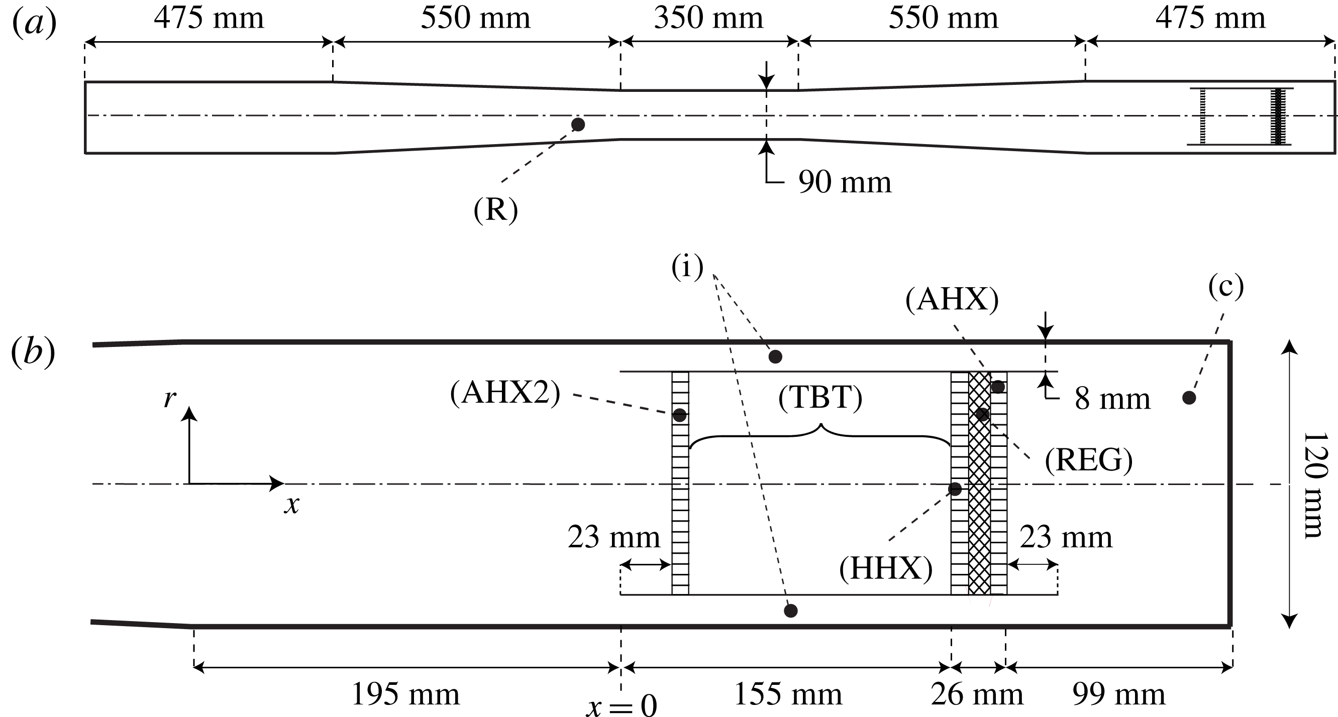
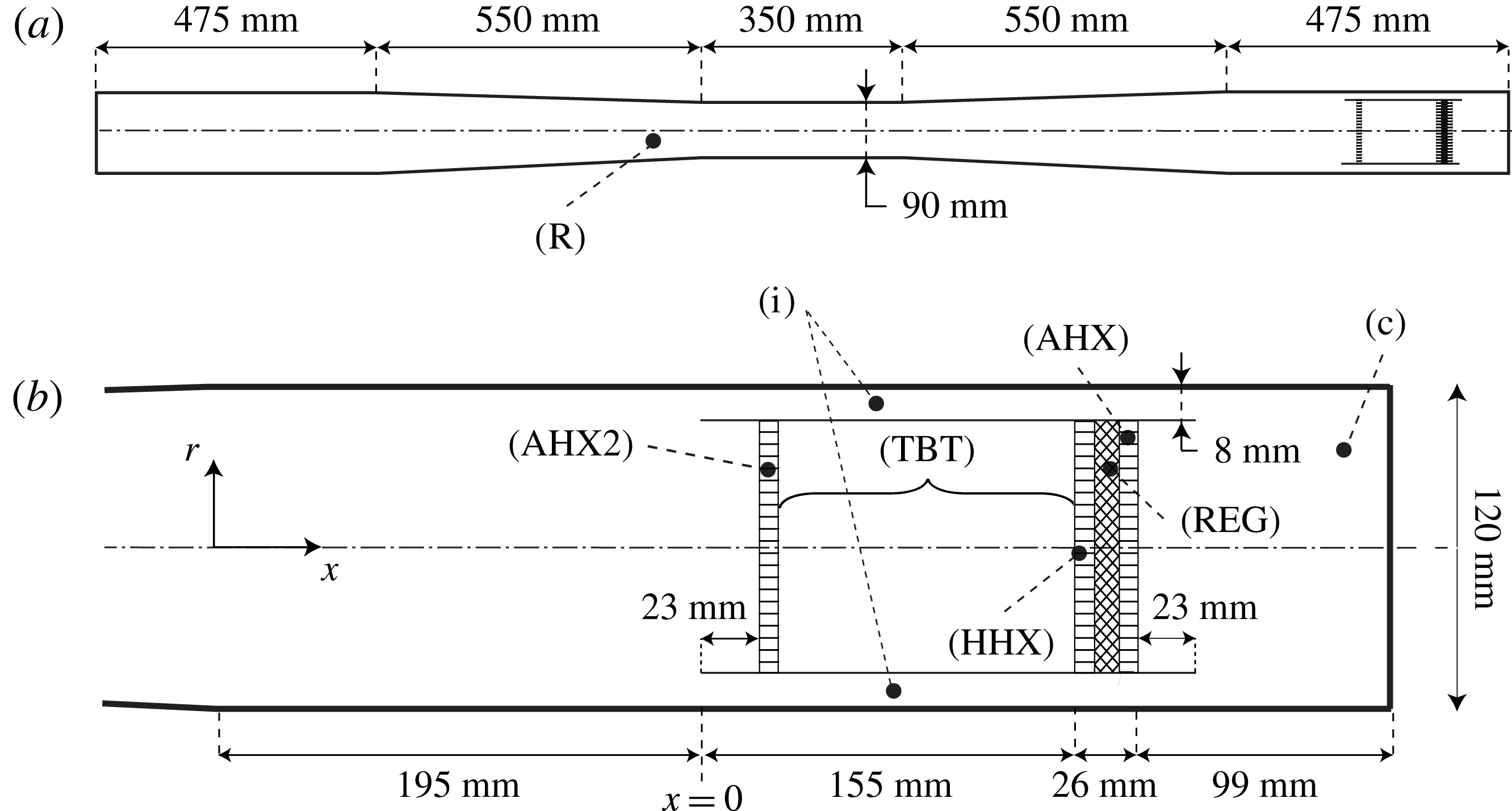
, respectively, for all cases. The equations are solved in the geometry illustrated in figure 1, consisting of a long resonator with the REG/HX unit at one end, enclosed by a zero-thickness annular tube, which is also referred to as the pulse tube. The section of the pulse tube between the HHX and the AHX2 is the TBT. The resonator and annular tube are treated as adiabatic no-slip walls with homogeneous Neumann conditions for pressure. While the choice of adiabatic wall conditions is consistent with the model of Lycklama à Nijeholt et al. (Reference Lycklama à Nijeholt, Tijani and Spoelstra2005) and reduces the overall complexity of the computational set-up, it does not allow one to account for thermal dissipation of acoustic energy in the boundary layer.
Illustration of the model travelling-wave TAE inspired by Lycklama à Nijeholt et al. (Reference Lycklama à Nijeholt, Tijani and Spoelstra2005). Full system (a) and REG/HX area (b), drawn to scale. A dash-dotted line indicates the line of symmetry. The different components of the engine are the resonator (R), the annular feedback inertance loop (i), the compliance (c), the hot heat exchanger (HHX), the regenerator (REG), the ambient heat exchanger (AHX), secondary heat exchanger (AHX2) and the thermal buffer tube (TBT). The annular tube enclosing the AHX2, HHX, REG and AHX is also referred to as the pulse tube, of which the TBT is only a section.
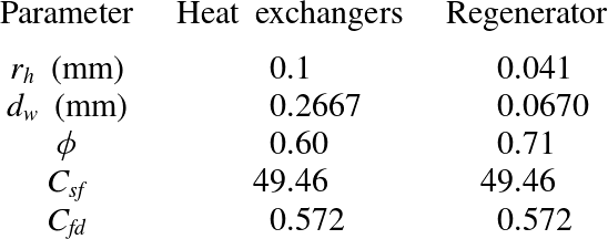
The REG and HXs are typically composed of a porous metallic structure ranging from overlapped wire screens (or metal felts) to stacks of parallel plates or rods, the former being more typical for REGs, the latter for HXs. Following Lycklama à Nijeholt et al. (Reference Lycklama à Nijeholt, Tijani and Spoelstra2005) we choose to model the heat transfer and drag in such components via the source terms
 $D_{i}$
and
 $S_{E}$
on the right-hand side of (2.1b
) and (2.1c
). They are expressed as
 $$\begin{eqnarray}\displaystyle & D_{i}=-[R_{C}+R_{F}(u_{j}u_{j})^{1/2}]u_{i}, & \displaystyle\end{eqnarray}$$
 $$\begin{eqnarray}\displaystyle & S_{E}=-u_{i}D_{i}+S_{h}, & \displaystyle\end{eqnarray}$$
 $D_{i}$
is modelled following the parametrizations
 $$\begin{eqnarray}\displaystyle & \displaystyle R_{C}=C_{sf}{\it\mu}\frac{(1-{\it\phi})}{4{d_{w}}^{2}{\it\phi}}, & \displaystyle\end{eqnarray}$$
 $$\begin{eqnarray}\displaystyle & \displaystyle R_{F}=\frac{{\it\rho}C_{fd}}{4d_{w}}, & \displaystyle\end{eqnarray}$$
 ${\it\phi}$
and
 $d_{w}$
are the characteristic porosity and mesh wire size of the component, and
 $C_{sf}$
and
 $C_{fd}$
are dimensionless fitting constants taken from the ILK Dresden and Kühl metal felts correlations (Thomas & Pittman Reference Thomas and Pittman2000). These are specific to TAE REGs and are derived under different oscillating flow conditions. Unfortunately, Lycklama à Nijeholt et al. (Reference Lycklama à Nijeholt, Tijani and Spoelstra2005) does not provide values for the wire size
 $d_{w}$
, which have been estimated according to (Organ Reference Organ1992)
 $$\begin{eqnarray}r_{h}=\frac{d_{w}{\it\phi}}{4(1-{\it\phi})},\end{eqnarray}$$
where
 $r_{h}$
is the pore hydraulic radius.
The source term
 $S_{h}$
in (2.3b
) accounts for heat transfer in the REG/HX unit and is modelled as
 $$\begin{eqnarray}S_{h}=-{\it\alpha}_{T}[T-T_{0}(x)],\end{eqnarray}$$
where
 $T$
is the instantaneous fluid temperature and
 $T_{0}(x)$
is the target mean temperature profile, which is equal to
 $T_{h}$
and
 $T_{a}$
, respectively, in the HHX and AHX, and varies linearly in the REG between the two values. No information is provided in Lycklama à Nijeholt et al. (Reference Lycklama à Nijeholt, Tijani and Spoelstra2005) for the proportionality constant
 ${\it\alpha}$
. We propose to model it as (R. Hixon, Personal communication, 2012)
 $$\begin{eqnarray}{\it\alpha}_{T}={\it\alpha}_{h}\frac{{\it\rho}R}{{\it\gamma}-1},\end{eqnarray}$$
where
 $R$
is the gas constant and
 ${\it\gamma}$
is the ratio of specific heats. The ratio
 ${\it\rho}R/({\it\gamma}-1)$
in (2.6) is a ballpark estimate of variations of total energy with respect to temperature (
 $\partial {\it\rho}E_{t}/\partial T$
) derived using the equation of state. The constant
 ${\it\alpha}_{h}$
is defined as
 $$\begin{eqnarray}{\it\alpha}_{h}=1/{\it\tau}_{h},\end{eqnarray}$$
where
 ${\it\tau}_{h}$
is the characteristic time scale for heat transfer in the void spaces of the HXs and REG. An estimate for
 ${\it\tau}_{h}$
can be derived by modelling such components as stacks of parallel plates with spacing
 $b$
matching the given hydraulic radius of the pores,
 $b=2r_{h}$
(table 1). This results in (Bejan Reference Bejan2004)
 $$\begin{eqnarray}{\it\tau}_{h}=\frac{(b/2)^{2}}{k/{\it\rho}C_{p}}=\frac{b^{2}{\it\rho}Pr}{4{\it\mu}},\end{eqnarray}$$
where
 $k$
is the thermal conductivity and
 $C_{p}$
the specific heat capacity of the gas.
This simplified model is expected to predict the intensity of the heat-transfer rate to the pore flow within an order of magnitude. It is based on the assumption of perfect thermal contact and is in quantitative agreement with a similar model used in DeltaEC (Ward & Swift Reference Ward and Swift1994). While the thermal regime resulting from (2.6) is not affected by the flow velocity, its linear dependency on the temperature facilitates the lower-order modelling efforts made in the present manuscript. Overall, despite their simplicity and coarse approximation, the application of the source terms (2.3) reproduces the essential thermodynamic and hydrodynamic processes that occur in REGs and HXs in TAEs, as discussed in the following.
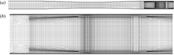
Cross-section of three-dimensional computational grid A for the full length resonator (a) and zoom on the right end (b) corresponding to the view in figure 1. The computational grid has been mirrored about the centreline for illustrative purposes. Computations are performed in a
 $90^{\circ }$
sector.

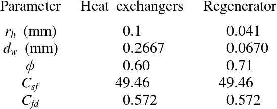
Parameters for REG/HX model (2.3). Hydraulic radius
 $r_{h}$
, characteristic wire diameter
 $d_{w}$
(mm), porosity
 ${\it\phi}$
and drag coefficients
 $C_{sf}$
,
 $C_{fd}$
(Thomas & Pittman Reference Thomas and Pittman2000). Values for
 $r_{h}$
and
 ${\it\phi}$
are taken from Lycklama à Nijeholt et al. (Reference Lycklama à Nijeholt, Tijani and Spoelstra2005).
3. Numerical model
The governing equations are discretized on an unstructured hexahedral mesh (figure 2) and solved in a
 $90^{\circ }$
sector with rotational periodicity applied in the azimuthal direction. The infinitely thin annular tube wall is introduced by breaking the mesh connectivity, creating two overlapping boundary surfaces with opposite orientation. Three concentric
 $O$
-grids in the cross-section, two in the annular tube and one in the pulse tube (not shown), are required in this region to map the polar mesh at the resonator walls to a quasi-uniform Cartesian block at the centre. High resolution is retained near the sharp edges of the annular tube walls to properly capture the shear layer caused by periodic flow separation. Visual inspection of the flow in previous calculations does not reveal a significant vorticity magnitude away from the wall for
 $x<-0.1~\text{m}$
. This has led to the choice of collapsing hexahedral elements into larger ones (i.e. grid coarsening) starting at
 $x=-0.146~\text{m}$
(figure 2
b), resulting in a coarser radial grid distribution for
 $x<-0.146~\text{m}$
. Points have also been concentrated in the AHX2 (
 $x=0.031~\text{m}$
), due to intense instantaneous temperature and velocity gradients at the limit cycle created by hot fluid streaming away from the HHX (discussed later). Overall, a significant effort has been made to retain a high-quality structured grid when possible.
A preliminary grid refinement study has been carried out to ensure adequate resolution of the axially symmetric components of the acoustic field and accurate prediction of the growth rate. The latter is sensitive primarily to the resolution in the axial direction (main direction of propagation of the acoustic waves), both in the resonator and in the TBT. The viscous boundary layers are resolved with a control-volume height of 0.1 mm at the wall for all cases. These considerations have lead to the design of a baseline grid distribution, grid A (figure 2), used to rapidly advance in time through the initial transient. Simulations have been carried out for HHX temperatures of
 $T_{h}=440$
, 460, 480 and 500 K and an AHX temperature of
 $T_{a}=300~\text{K}$
in all cases. The acoustic perturbation is initialized with a standing wave of 0.5 kPa in amplitude and the source terms (2.3) are applied from the beginning. The former is only used to reduce the duration of the transient and is not required to achieve acoustic energy growth (see § 4). Once a limit cycle is reached, two successive grid refinement steps are carried out, resulting in grids B and C. At each step the resolution was increased in the axial direction, especially around the sharp edges, and systematically doubled in the azimuthal direction. The effective resolution in the latter direction is equivalent to Wu & Moin (Reference Wu and Moin2008)’s direct numerical simulation of pipe flow at comparable Reynolds numbers. The mesh size in the radial direction is then adjusted and/or increased to optimize the cell’s aspect ratio. The sensitivity of the wave-induced Reynolds stresses to these changes (shown later) is used as a metric for grid convergence and has only been assessed in calculations at
 $T_{h}=500~\text{K}$
(table 2).
Parameter space for numerical simulations carried out to limit cycle. Total number of control volumes
 $N_{cv}$
, control volumes in the azimuthal direction only
 $N_{{\it\theta}}$
, temperature in the HHX
 $T_{h}$
. For all cases
 $T_{a}=300~\text{K}$
. Three meshes with increasing level of resolution and quality (from grid A to C) are considered. Computations performed (x) and not performed (
 $\cdot$
).

The governing equations for mass, momentum and total energy are solved in the finite-volume unstructured code
 $\text{CharLES}^{\text{X}}$
, developed as a joint-effort project among researchers at Stanford University. The flux reconstruction method is grid-adaptive at the preprocessing stage and solution-adaptive at run time. It blends a high-order polynomial interpolation scheme (up to fourth-order on uniform meshes) with a lower-order scheme to ensure numerical stability in areas of low grid quality (Ham et al.
Reference Ham, Mattsson, Iaccarino and Moin2007). A second-order, essentially non-oscillatory (ENO) reconstruction is adopted within the TBT to control unwanted oscillations in the solution caused by the application of the source terms (2.3). The discretized system of equations is integrated in time with a fully explicit, third-order Runge–Kutta scheme. The code is parallelized using the message passing interface (MPI) protocol and highly scalable on a large number of processors. The adoption of computationally intensive discretizations such as ENO reconstruction in a limited portion of the domain has lead to a load-balancing problem that required a volume-based dual-constrained partitioning (Karypis & Kumar Reference Karypis and Kumar1998; Schloegel, Karypis & Kumar Reference Schloegel, Karypis and Kumar2000) to recover acceptable performance.
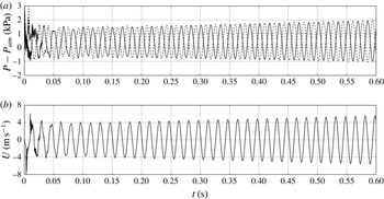
(a) Time series of pressure along the centreline,
 $r=0$
, at
 $x=-1.8825~\text{m}$
(– –) and
 $x=0.0425~\text{m}$
(—–) and (b) axial velocity at
 $x=-0.92~\text{m}$
(—–) for the case
 $T_{h}=500~\text{K}$
on grid A.

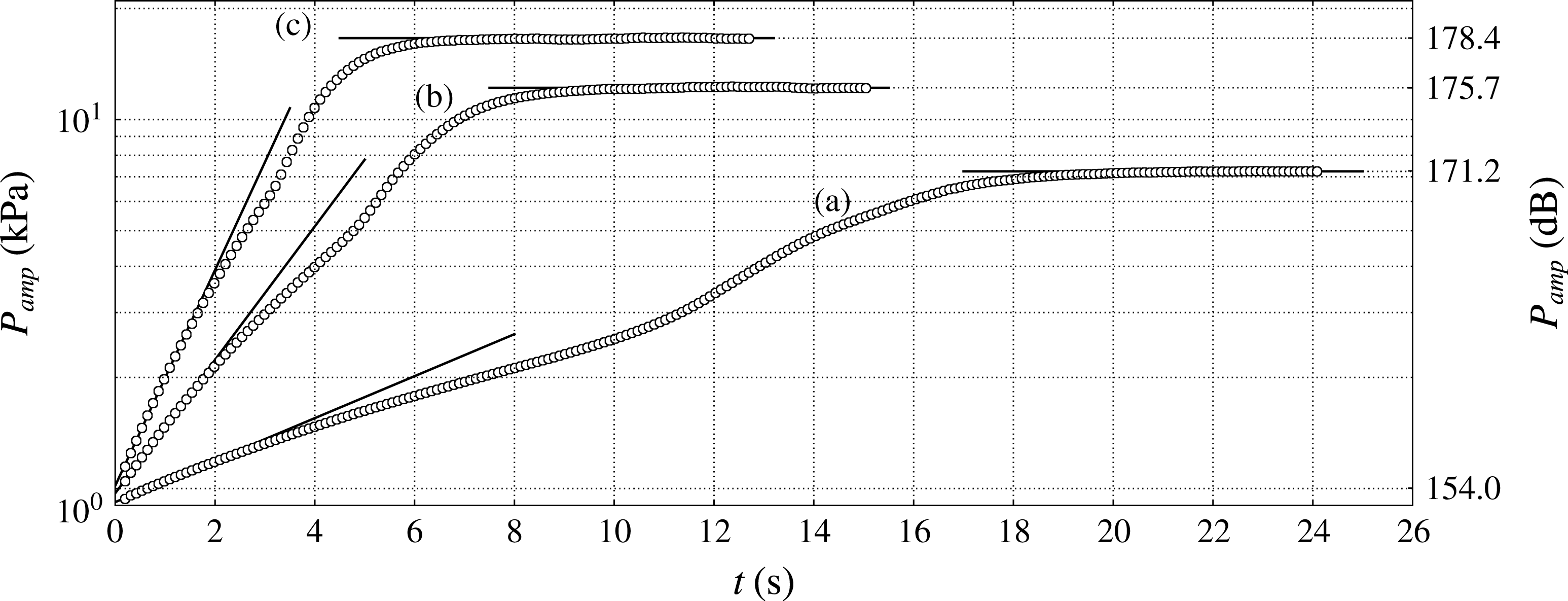
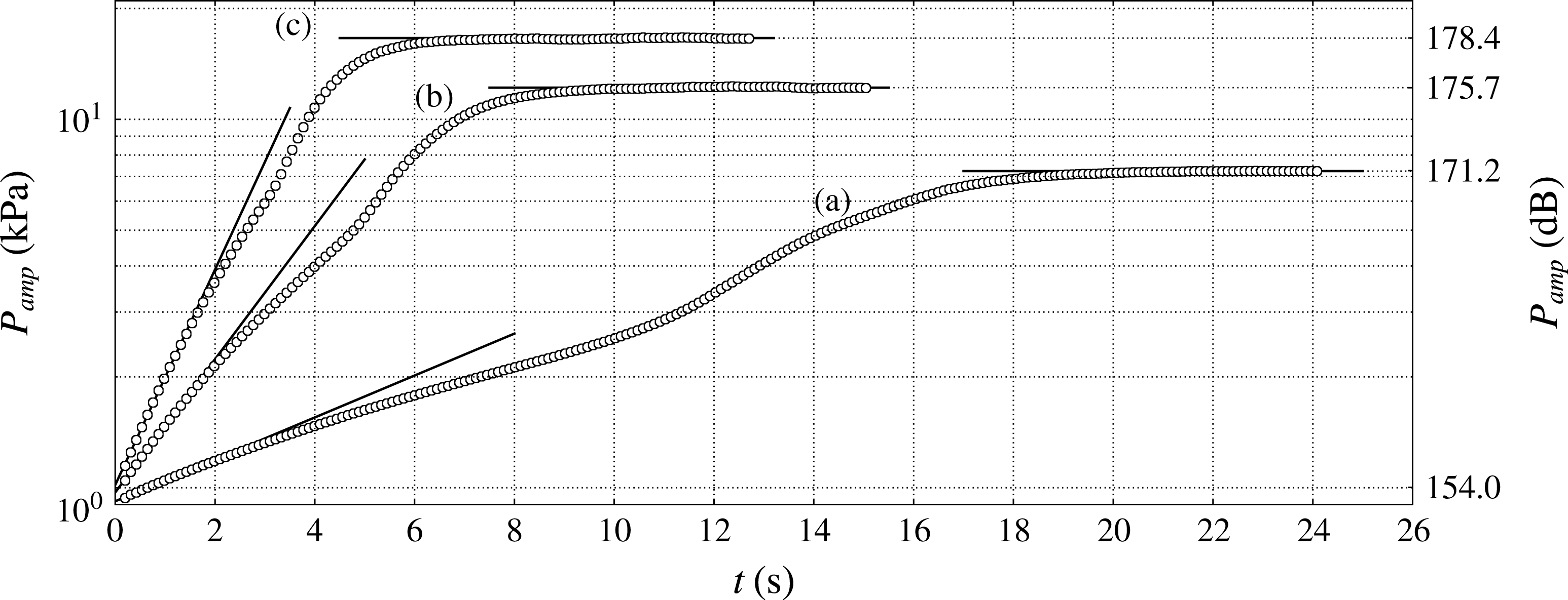
Time series of pressure amplitude (kPa) on the left end of the resonator and corresponding sound pressure level (
 $+$
dB) for
 $T_{h}=460~\text{K}$
(a),
 $T_{h}=480~\text{K}$
(b) and
 $T_{h}=500~\text{K}$
(c) on grid A (see table 2). The decaying case for
 $T_{h}=440~\text{K}$
is not shown.
4. Engine startup
In all of the numerical trials performed, the abrupt activation of the source terms (2.3) alone in a quiescent flow provides a sufficiently intense initial disturbance (
 ${\sim}$
1 kPa) to trigger the thermoacoustic instability, leading to the production of acoustic energy in the system (figures 3 and 4). Several attempts have been made to reduce the initial pressure amplitude, but have not been successful. In order to rapidly damp the broadband component of such a disturbance, all cases are initiated with a half-wavelength pressure distribution of 0.5 kPa in amplitude, with base pressure and temperature of 101 325 Pa and 300 K. For a given hot temperature setting, the pressure amplitude initially grows exponentially at the same rate and frequency (
 ${\sim}$
60 Hz) at all locations in the engine. As shown later in § 4.3, the observed behaviour (in the first few seconds of operation) can be quantitatively explained with a system-wide model based solely on linear acoustics.
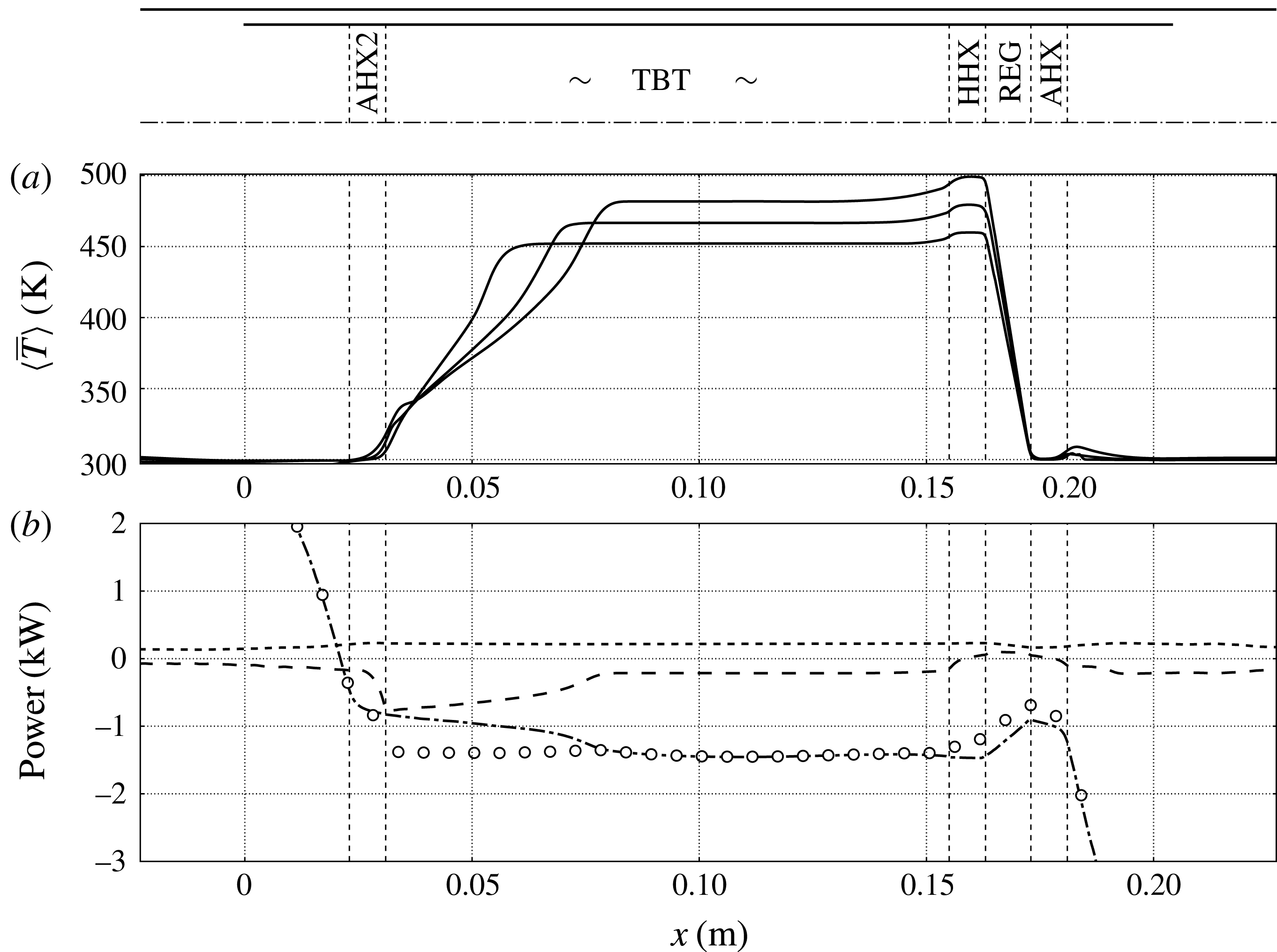
The rapidly growing pressure amplitude is accompanied by an increasing base pressure (not shown). The latter is caused by the gradual leakage of hot fluid in the TBT from the HHX (a nonlinear effect), already visible in the startup phase (figure 5
a, for
 $x<0.155~\text{m}$
). While such an effect is not important during the first seconds of operation, it affects the growth rate at later times. As the slowly advancing (cycle-averaged) hot flow front enters into contact with the AHX2 for the first time, a sudden increase in the growth rate is observed. At the same time, the base pressure plateaus due to the AHX2 picking up the excess heat. Finally, the acoustic pressure amplitude settles after the overall dissipation matches the enhanced acoustic energy production. These are all nonlinear effects, which will be discussed in more detail in § 5. In the following we restrict the analysis of the generation and propagation of acoustic energy in the system during the startup phase to linear acoustics.
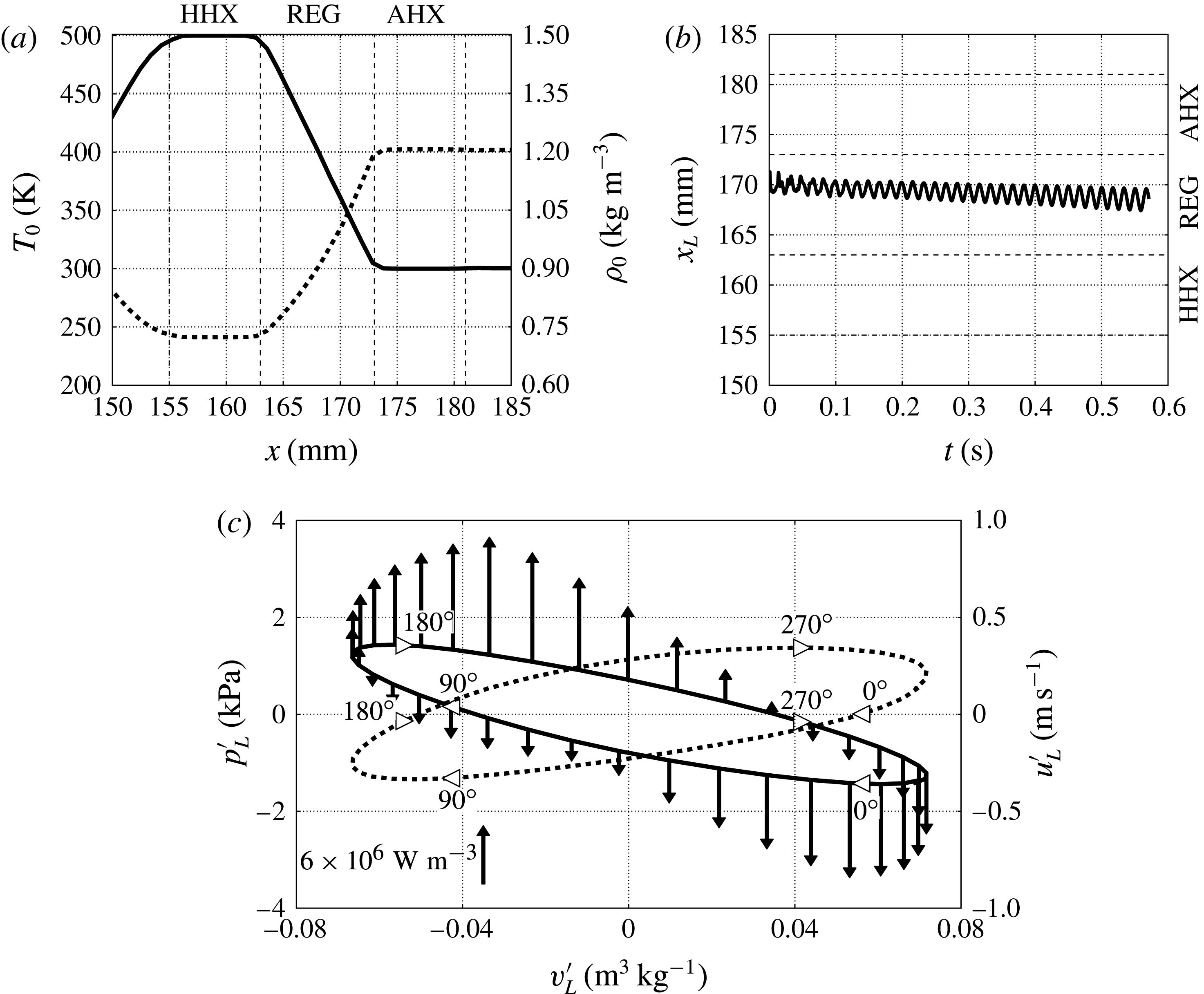
(a) Base temperature (—–) and density profiles (- - -) taken along the centreline in the REG/HX unit at
 $t=0.55~\text{s}$
for
 $T_{h}=500~\text{K}$
, grid A (see table 2); (b) Lagrangian fluid parcel axial position
 $x_{L}$
starting at
 $x=0.171~\text{m}$
at
 $t=0$
; (c) fluctuating pressure,
 $p_{L}^{\prime }$
, (—–) and velocity,
 $u_{L}^{\prime }$
, (- - -) of the Lagrangian fluid parcel in (b) plotted against specific volume fluctuation,
 $v_{L}^{\prime }$
, over one acoustic cycle at
 $t=0.55~\text{s}$
with heat release fluctuation,
 ${S_{h}}^{\prime }$
(2.6) shown with arrows (oriented upwards for heat addition
 $S_{h}^{\prime }>0$
and downwards for removal
 $S_{h}^{\prime }<0$
with scale in figure). Both cycles are traversed clockwise, as shown by the phase markers.
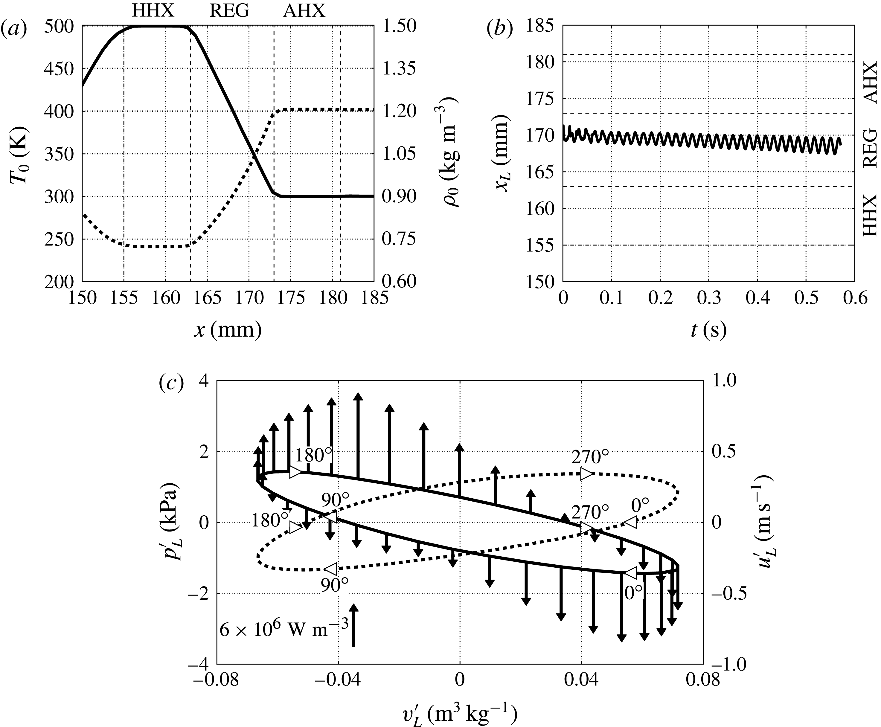
The driver of the thermoacoustic instability, converting heat into acoustic power, is the mean temperature gradient imposed in the REG/HX unit (figure 5 a). Insight into the fundamental energy conversion mechanisms can be gained by looking at the evolution of a Lagrangian fluid parcel in the REG interacting with the acoustic field. The slight drift in the direction of the mean temperature gradient (figure 5 b) is a nonlinear effect known as acoustic streaming (discussed later in § 5), which can be ignored at this stage.
The fluid parcel in the REG experiences a thermodynamic cycle converting heat into acoustic power, which is neither the ideal Stirling or Carnot cycle (figure 5 c). For example, purely isochoric transformations, present in the ideal Stirling cycle, are not possible due to the sinusoidal waveform of the acoustic velocity and pressure. Moreover, isentropic transformations, present in the ideal Carnot cycle, are not possible due to the heat-exchange and viscous losses in the REG/HX unit. However, analogously to the ideal Stirling cycle, most of the heating and cooling occurs, respectively, during the expansion and compression stages. The heat-transfer model in (2.6) assumes perfect thermal contact and it is therefore likely that its adoption leads to an overestimation of the real thermoacoustic response under comparable conditions.
Due to the orientation of the background temperature gradient (
 $\text{d}T_{0}(x)/\text{d}x<0$
, figure 5
a), a fluid parcel in the REG that is displaced towards the HHX (
 $u^{\prime }<0$
) will experience heating. This occurs with a given phase lag with respect to the velocity depending, in particular, on the nature of the heat transfer. In our case the heat addition,
 $S_{h}^{\prime }>0$
, peaks
 ${\sim}90^{\circ }$
after the maximum negative velocity (at which point the parcel comes to rest) and so does the positive pressure fluctuation,
 $p^{\prime }>0$
(figure 5
c). The opposite occurs when the fluid is displaced towards the AHX. Consistently with the energetic considerations underlying the Rayleigh criterion,
 $\overline{S_{h}^{\prime }p^{\prime }}>0$
, the observed phase differences suggest the presence of positive acoustic energy production. The phasing between velocity and pressure fluctuations is consistent with a standing wave, short of approximately 15°. This slight phase difference contributes to a negative correlation between
 $u^{\prime }$
and
 $p^{\prime }$
, i.e. the left-travelling wave propagating through the REG/HX is more intense than the right-travelling wave. Acoustic power is therefore being produced.
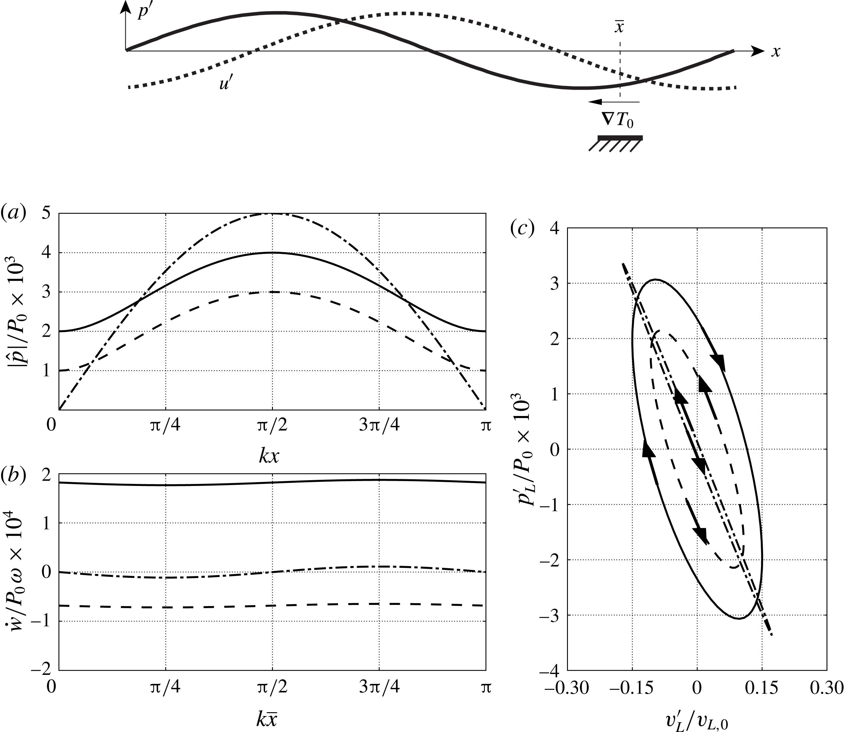
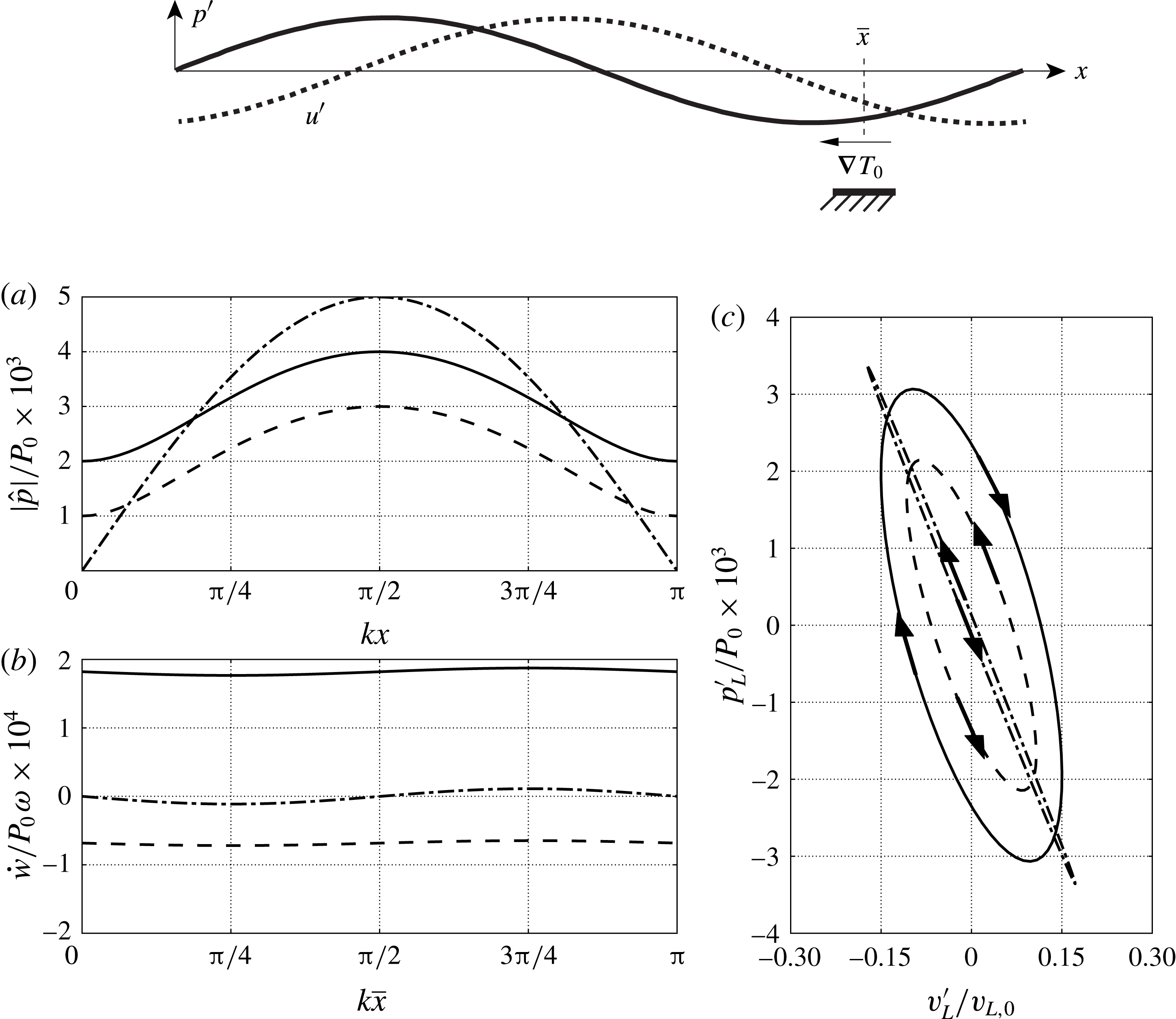
Results from the linear Lagrangian model (§ 4.1) applied to a one-dimensional theoretical TAE (inspired by Swift Reference Swift1988) composed of a generic plane wave interacting with a negative temperature gradient located at
 $\overline{x}$
(top). (a) Imposed pressure distribution as a function of
 $kx$
, (b) overall cycle-averaged work (i.e. generated acoustic power) as a function of
 $k\overline{x}$
(temperature gradient location) and (c) Lagrangian thermodynamic cycle extracted in the temperature gradient region for
 $k\overline{x}={\rm\pi}/4$
(c). Results for plane waves of amplitude
 $p^{-}=3\times 10^{-3}P_{0}$
,
 $p^{+}=1\times 10^{-3}P_{0}$
(—–);
 $p^{+}=p^{-}=2.5\times 10^{-3}P_{0}$
(— ⋅ —);
 $p^{-}=1\times 10^{-3}P_{0}$
,
 $p^{+}=3\times 10^{-3}P_{0}$
(– –) for
 $P_{0}={\it\rho}_{0}a_{0}^{2}$
. For all cases
 ${\it\phi}^{-}={\it\phi}^{+}=-{\rm\pi}/2$
.
4.1. A Lagrangian model of the thermodynamic cycle
Inspired by Swift (Reference Swift1988)’s theoretical TAE (figure 6, top), a one-dimensional analytical model is derived in the following to rigorously explain the interaction between a mean temperature gradient and a Lagrangian fluid parcel in a generic planar acoustic wave field. The latter can be expressed as the linear superposition of a left- and a right-travelling wave, which in complex form reads
 $$\begin{eqnarray}\displaystyle & \hat{p}(x)=p^{-}\text{e}^{\text{i}[kx+{\it\phi}^{-}]}+p^{+}\text{e}^{\text{i}[-kx-{\it\phi}^{+}]}, & \displaystyle\end{eqnarray}$$
 $$\begin{eqnarray}\displaystyle & {\it\rho}_{0}a_{0}\hat{u} (x)=-p^{-}\text{e}^{\text{i}[kx+{\it\phi}^{-}]}+p^{+}\text{e}^{\text{i}[-kx-{\it\phi}^{+}]}, & \displaystyle\end{eqnarray}$$
 $p^{+/-}$
and
 ${\it\phi}^{+/-}$
are the amplitude and phase of the right/left-travelling wave and
 $k$
is the wavenumber. The acoustic pressure and velocity in time are given based on the convention
 $p^{\prime }=\hat{p}(x)\text{e}^{\text{i}{\it\omega}t}$
and
 $u^{\prime }=\hat{u} (x)\text{e}^{\text{i}{\it\omega}t}$
, where
 $\text{i}$
is the imaginary unit and the base impedance
 ${\it\rho}_{0}a_{0}$
is given by the state
 $\{{\it\rho}_{0},T_{0},P_{0}\}$
.
Let
 $x_{p}=\overline{x}+x_{p}^{\prime }$
be the instantaneous position of a fluid parcel oscillating with small displacements
 $x_{p}^{\prime }$
about the position
 $\overline{x}$
, where a linear temperature gradient is locally imposed (figure 6). The fluid parcel velocity can be approximated, based on the assumption
 $k\max (x_{p}^{\prime })\ll 1$
, as
 $$\begin{eqnarray}\frac{\text{d}}{\text{d}t}x_{p}^{\prime }=u^{\prime }(\overline{x}+x_{p}^{\prime },t)=\text{Re}\{\hat{u} (\overline{x}+x_{p}^{\prime })\text{e}^{\text{i}{\it\omega}t}\}\simeq \text{Re}\{\hat{u} (\overline{x})\text{e}^{\text{i}{\it\omega}t}\},\end{eqnarray}$$
yielding the relation
 $$\begin{eqnarray}\hat{x}_{p}=\hat{u} (\overline{x})/\text{i}{\it\omega}.\end{eqnarray}$$
Introducing a Lagrangian base state
 ${\it\rho}_{L,0},P_{L,0},T_{L,0}$
(specified later) for the fluid parcel density, entropy and temperature,
 $$\begin{eqnarray}\displaystyle & {\it\rho}_{L}={\it\rho}_{L,0}+\text{Re}\{\hat{{\it\rho}}_{L}\text{e}^{\text{i}{\it\omega}t}\}, & \displaystyle\end{eqnarray}$$
 $$\begin{eqnarray}\displaystyle & s_{L}=s_{L,0}+\text{Re}\{{\hat{s}}_{L}\text{e}^{\text{i}{\it\omega}t}\}, & \displaystyle\end{eqnarray}$$
 $$\begin{eqnarray}\displaystyle & T_{L}=T_{L,0}+\text{Re}\{\hat{T}_{L}\text{e}^{\text{i}{\it\omega}t}\}, & \displaystyle\end{eqnarray}$$
 $x_{p}$
, yields
 $$\begin{eqnarray}{\it\rho}_{L}T_{L}\frac{\text{d}s_{L}}{\text{d}t}=-{\it\alpha}_{T}[T_{L}-T_{0}(x_{p})],\end{eqnarray}$$
where the (total) time derivative on the left-hand side, applied to the Lagrangian fluid parcel’s specific entropy, has replaced the material derivative of the Eulerian entropy field.
Substituting Gibbs’ relationship linearized about the Lagrangian base state
 $T_{L,0},p_{L,0}$
(
 $=p_{0}$
),
 $$\begin{eqnarray}\text{d}s_{L}=\frac{c_{p}}{T_{L,0}}\text{d}T_{L}-\frac{R}{p_{0}}\text{d}p_{L},\end{eqnarray}$$
into (4.8), which is also linearized assuming
 ${\it\rho}_{L}T_{L}\simeq {\it\rho}_{L,0}T_{L,0}$
, yields
 $$\begin{eqnarray}{\it\rho}_{L,0}c_{p}\frac{\text{d}T_{L}}{\text{d}t}-\frac{\text{d}p_{L}}{\text{d}t}=-{\it\alpha}_{T}[T_{L}-T_{0}(x_{p})].\end{eqnarray}$$
The imposed mean temperature at the particle location,
 $T_{0}(x_{p})$
, can be expressed via the Taylor expansion
 $$\begin{eqnarray}T_{0}(x_{p})=T_{0}(\bar{x})+\left.x_{p}^{\prime }\frac{\text{d}T_{0}}{\text{d}x}\right|_{x=\bar{x}}\end{eqnarray}$$
which is exact in the case of a linear base temperature distribution. Substituting (4.11) into (4.10) yields
 $$\begin{eqnarray}{\it\rho}_{L,0}c_{p}\frac{\text{d}T_{L}}{\text{d}t}-\frac{\text{d}p_{L}}{\text{d}t}=-{\it\alpha}_{T}\left[T_{L}-T_{0}(\bar{x})-\left.x_{p}^{\prime }\frac{\text{d}T_{0}}{\text{d}x}\right|_{x=\bar{x}}\right].\end{eqnarray}$$
Defining the Lagrangian-based state for temperature such that
 $T_{L,0}=T_{0}(\overline{x})$
, assuming
 $p_{L}=p$
and switching to the complex form,
 $$\begin{eqnarray}{\it\rho}_{L,0}c_{p}\text{i}{\it\omega}\hat{T}_{L}-\text{i}{\it\omega}\hat{p}=-{\it\alpha}_{T}\left[\hat{T}_{L}-\left.\hat{x}_{p}\frac{\text{d}T_{0}}{\text{d}x}\right|_{x=\bar{x}}\right],\end{eqnarray}$$
where the Lagrangian base density is
 ${\it\rho}_{L,0}=p_{0}/(RT_{L,0})$
.
If the acoustic field is assigned, so are the complex pressure amplitude
 $\hat{p}$
and particle displacement
 $\hat{x}_{p}=(\text{i}{\it\omega})^{-1}\hat{u} (\overline{x})$
, which then allows one to solve for
 $\hat{T}_{L}$
from (4.13). The density of the Lagrangian parcel can then be calculated from the linearized equation of state
 $$\begin{eqnarray}\hat{{\it\rho}}_{L}=\frac{\hat{p}-{\it\rho}_{L,0}R\hat{T}_{L}}{RT_{L,0}}.\end{eqnarray}$$
The work done by the fluid parcel on the surrounding ambient per unit time (generated acoustic power) is
 $$\begin{eqnarray}{\dot{w}}=-\overline{\frac{p}{{\it\rho}}\frac{\text{D}{\it\rho}}{\text{D}t}}\simeq -\frac{1}{{\it\rho}_{L,0}}\frac{1}{2}\text{Re}\{\hat{p}(\text{i}{\it\omega}\hat{{\it\rho}}_{L})^{\ast }\}.\end{eqnarray}$$
Depending on the nature of acoustic wave being imposed (figure 6
a), ranging from purely left-travelling to purely right-travelling, a different phasing between
 $\hat{p}$
and
 $\hat{u}$
is achieved, determining
 ${\dot{w}}$
(figure 6
b). In the case of a standing wave, acoustic energy will be absorbed (
 ${\dot{w}}<0$
) or generated (
 ${\dot{w}}>0$
) depending on the location of the temperature gradient,
 $\overline{x}$
. For a sufficiently high amplitude of the right-,
 $p^{+}\gg p^{-}$
, (or left-,
 $p^{-}\gg p^{+}$
) travelling wave, acoustic power is ultimately only absorbed (or generated) for any
 $\overline{x}$
in the case of a negative mean temperature gradient,
 $\text{d}T_{0}/\text{d}x<0$
(figure 6
b). This shows that an acoustic wave travelling in the same direction as or opposite to the imposed mean temperature gradient (applied over a region small compared to the wavelength) will be amplified or absorbed, respectively. Moreover, the acoustic power associated with the energy conversion occurring in an (almost) purely travelling wave is remarkably higher (see area enclosed by the
 $p{-}v$
diagrams in figure 6
c) than that of a standing wave of comparable amplitude. This confirms Ceperley (Reference Ceperley1979)’s seminal intuition that led to the revolutionary concept of travelling-wave energy conversion, trumping thereafter designs based on standing waves.
4.2. Acoustic network of travelling waves
In spite of the finite amplitude of the initial perturbation (exceeding 1 % of the base pressure) and the immediate establishment of nonlinear effects, the exponentially growing acoustic amplitude (with uniform growth rate in the entire system) suggests that the system-wide behaviour in the startup phase can be analysed by invoking linear acoustics. The low frequencies observed in the numerical simulations and the high aspect ratio of the resonator (with lowest cut-on frequency
 ${\sim}$
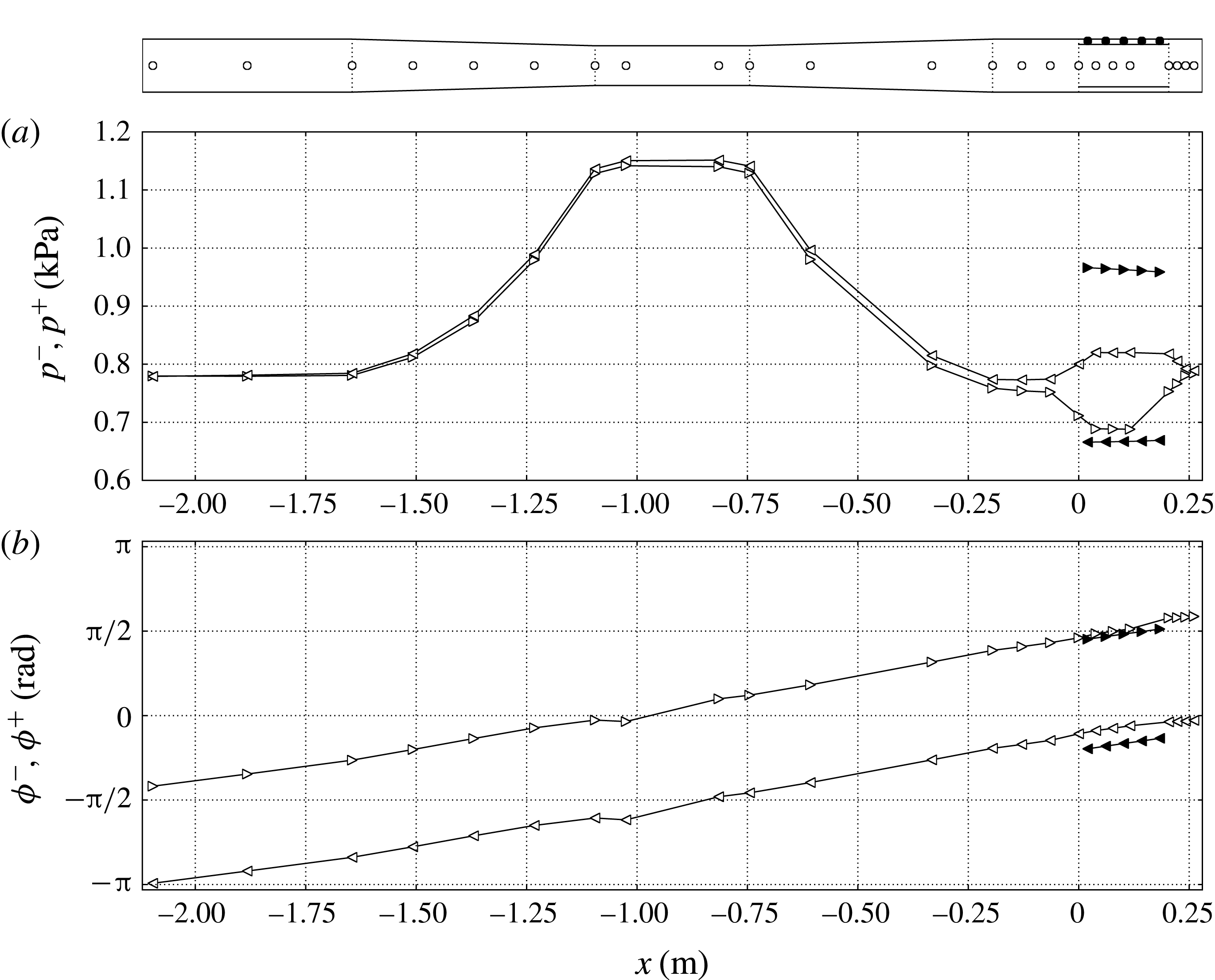
1.7 kHz) allows us to neglect radial or azimuthal acoustic modes at the resonator scale. This suggests that, as a first approximation, our analysis can be restricted to planar waves. The nature of the thermoacoustic instability in the REG/HX (analysed in § 4.1) suggests that the pulse tube acts as an amplifier of left-travelling waves. These are expected to propagate into the resonator, be reflected back and, upon returning to the REG/HX unit as right-travelling waves, propagate both through the pulse tube and in the feedback inertance (figure 1), being absorbed in the former case (figure 6
c) and propagating freely in the latter. The acoustic power propagating through the inertance is looped back into the REG/HX unit via the compliance, hence creating a network of self-amplified travelling waves. This scenario, typical of travelling-wave TAEs built in a looped configuration (Backhaus & Swift Reference Backhaus and Swift2000), is confirmed in the following analysis.
An exact local decomposition in terms of left
 $(-)$
and right
 $(+)$
travelling waves
 $$\begin{eqnarray}\displaystyle & p^{\prime }(t)=p^{-}f({\it\omega}t+{\it\phi}^{-})+p^{+}f(-{\it\omega}t+{\it\phi}^{+}), & \displaystyle\end{eqnarray}$$
 $$\begin{eqnarray}\displaystyle & u^{\prime }(t)=-u^{-}f({\it\omega}t+{\it\phi}^{-})+u^{+}f(-{\it\omega}t+{\it\phi}^{+}), & \displaystyle\end{eqnarray}$$
 $p^{\pm }$
and
 $u^{\pm }$
and phases
 ${\it\phi}^{\pm }$
of purely travelling waves of a given generic waveform
 $f(\,)$
(periodic function of period
 $2{\rm\pi}$
). In our case, the angular frequency
 ${\it\omega}$
is much larger than the growth rate (discussed in § 4.3), allowing us to ignore the variations of pressure and velocity amplitudes over one acoustic period as well as the change in base impedance,
 ${\it\rho}_{0}a_{0}$
, due to a DC mode in pressure (discussed above). The following analysis is restricted to the startup phase and for locations in the engine outside of the REG/HX unit where the strong mean temperature causes non-negligible spatial gradients of the base impedance and the isentropic wave propagation assumption to be violated.
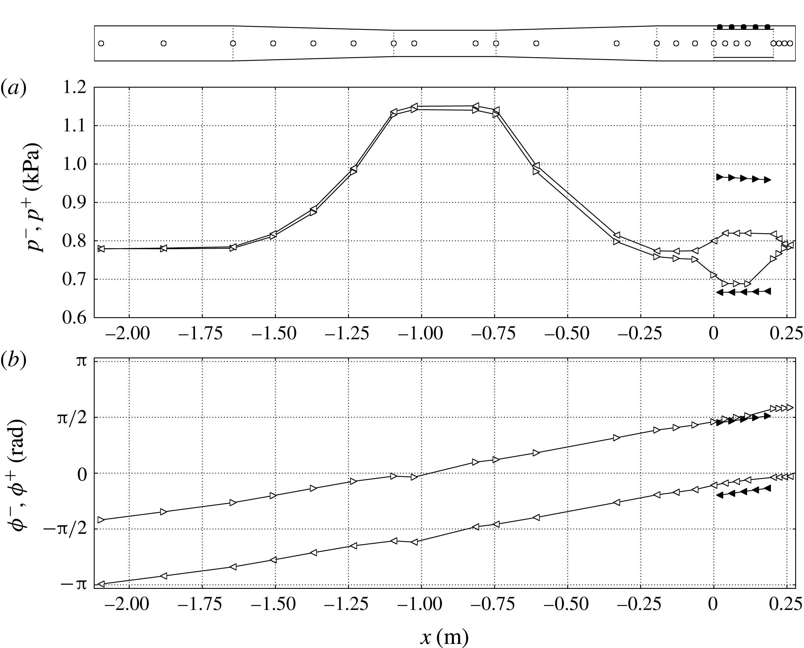
Left (–, ◃, ◂) and right (
 $+$
, ▹, ▸) travelling-wave amplitudes,
 $p^{\pm }$
, (a) and phases,
 ${\it\phi}^{\pm }$
, (b) extracted from the Navier–Stokes calculations based on the linear approximation (4.16) for time
 $t=0.55~\text{s}$
for the
 $T_{h}=500~\text{K}$
case on grid A. The locations where data is extracted are shown in the top subfigure. White and black symbols correspond to values extracted on the centreline and in the feedback inertance, respectively.
The acoustic perturbation (4.16) can be rewritten in the form of a complex Fourier series
 $$\begin{eqnarray}\displaystyle & \displaystyle \mathop{\sum }_{k=-\infty }^{+\infty }\hat{p}_{k}\text{e}^{\text{i}k{\it\omega}t}=p^{-}\mathop{\sum }_{k=-\infty }^{+\infty }\hat{f}_{k}\text{e}^{\text{i}k[{\it\omega}t+{\it\phi}^{-}]}+p^{+}\mathop{\sum }_{k=-\infty }^{+\infty }\hat{f}_{k}^{\ast }\text{e}^{\text{i}k[{\it\omega}t-{\it\phi}^{+}]}, & \displaystyle\end{eqnarray}$$
 $$\begin{eqnarray}\displaystyle & \displaystyle {\it\rho}_{o}a_{o}\mathop{\sum }_{k=-\infty }^{+\infty }\hat{u} _{k}\text{e}^{\text{i}k{\it\omega}t}=-p^{-}\mathop{\sum }_{k=-\infty }^{+\infty }\hat{f}_{k}\text{e}^{\text{i}k[{\it\omega}t+{\it\phi}^{-}]}+p^{+}\mathop{\sum }_{k=-\infty }^{+\infty }\hat{f}_{k}^{\ast }\text{e}^{\text{i}k[{\it\omega}t-{\it\phi}^{+}]}, & \displaystyle\end{eqnarray}$$
 $p^{\pm }=\pm {\it\rho}_{0}a_{0}u^{\pm }$
and the superscript
 $^{\ast }$
indicates the complex conjugate. Letting the
 $m$
th mode be any non-zero Fourier component, the unknowns
 $p^{\pm }$
and
 ${\it\phi}^{\pm }$
are easily determined by isolating that mode from (4.17), yielding
 $$\begin{eqnarray}\displaystyle & \displaystyle \hat{p}_{m}=\hat{f}_{m}[p^{-}\text{e}^{\text{i}m{\it\phi}^{-}}]+\hat{f}_{m}^{\ast }[p^{+}\text{e}^{-\text{i}m{\it\phi}^{+}}], & \displaystyle\end{eqnarray}$$
 $$\begin{eqnarray}\displaystyle & \displaystyle {\it\rho}_{o}a_{o}\hat{u} _{m}=-\hat{f}_{m}[p^{-}\text{e}^{\text{i}m{\it\phi}^{-}}]+\hat{f}_{m}^{\ast }[p^{+}\text{e}^{-\text{i}m{\it\phi}^{+}}]. & \displaystyle\end{eqnarray}$$
 $$\begin{eqnarray}\displaystyle & \displaystyle p^{-}=|\hat{p}_{m}-{\it\rho}_{0}a_{0}\hat{u} _{m}|/|2\hat{f}_{m}|, & \displaystyle\end{eqnarray}$$
 $$\begin{eqnarray}\displaystyle & \displaystyle p^{+}=|{\it\rho}_{0}a_{0}\hat{u} _{m}+\hat{p}_{m}|/|2\hat{f}_{m}^{\ast }|. & \displaystyle\end{eqnarray}$$
 ${\it\phi}^{-}$
and
 ${\it\phi}^{+}$
are then readily extracted from (4.18) given the pressure amplitudes
 $p^{-}$
and
 $p^{+}$
.
This procedure is applied to the discrete set of points in figure 7(top) located along the resonator axis and around the pulse tube. Results show that left-travelling waves leaving the REG/HX unit propagate into the resonator and are reflected back with a slightly lower amplitude due to losses in the resonator (figure 7 a). Consistently with the one-dimensional approximation in (4.16), the acoustic power can be expressed as
 $$\begin{eqnarray}{\dot{E}}_{a}^{+}=\int _{A}\overline{p^{\prime }u^{\prime }}\text{d}A=\frac{A}{{\it\rho}_{0}a_{0}}[{p^{+}}^{2}-{p^{-}}^{2}]\mathop{\sum }_{k=-\infty }^{+\infty }{\hat{f}_{k}}^{\ast }\hat{f}_{k},\end{eqnarray}$$
providing an energetic interpretation to the imbalance
 $p^{-}\gtrless p^{+}$
. The data (figure 7
a,b) confirm that, as anticipated earlier in this section, the acoustic power generated in the REG/HX is fed back to it by the compliance after being channelled through the inertance, where
 ${p^{+}}^{2}\gg {p^{-}}^{2}$
.
The adopted coaxial configuration is not efficient as it allows part of the acoustic power that is returned by the resonator to be absorbed by the pulse tube. This results in a spatial distribution of the phases
 ${\it\phi}^{-}$
and
 ${\it\phi}^{+}$
almost resembling a standing wave (figure 7
b). However, the clear deviation in the REG/HX and in the inertance from such a pattern, both in the phases,
 ${\it\phi}^{\pm }$
, and in the wave amplitudes,
 $p^{\pm }$
, is due to the acoustic energy production mechanisms illustrated in figure 5
c and modelled in § 4.1, which are based on the travelling-wave concept (Ceperley Reference Ceperley1979).
The presence of acoustic power being looped around the REG/HX unit (the feedback inertance), which is a component not found in standing-wave TAEs, effectively qualifies the proposed model as a travelling-wave TAE and, as discussed later in § 5, is directly responsible for nonlinear processes such as Gedeon streaming. If the same model had been rearranged in a looped configuration, the departure from a pure standing wave in the REG/HX unit and inertance would only be (quantitatively) more significant, while retaining the same (qualitative) structure as found in the present configuration.
4.3. System-wide linear modelling
Results shown so far suggest that nonlinearities do not play an important role in explaining the acoustic energy propagation and amplification mechanisms during the startup phase. However, given the high amplitude of the initial perturbation (
 ${\sim}1$
kPa) and the presence of complex geometrical features such as the sharp edges of the pulse tube (inducing vortex shedding from the start), it is important to assess to what extent a system-wide linear model is able to quantitatively explain the observed instability.
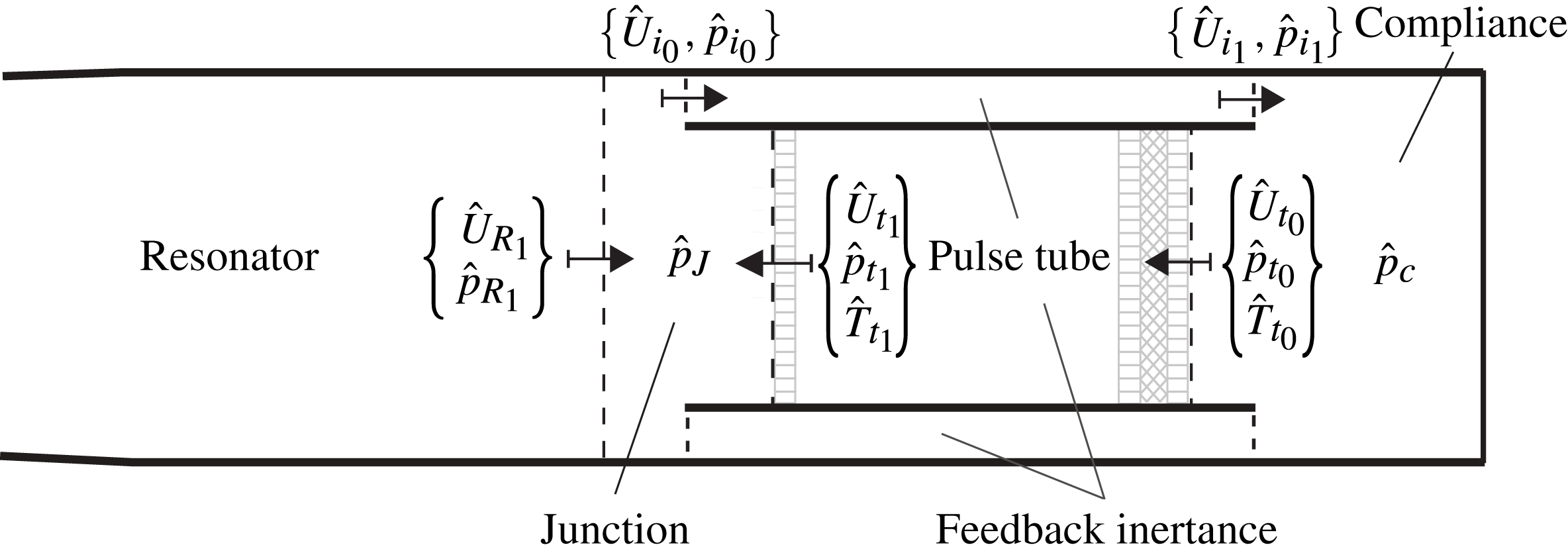
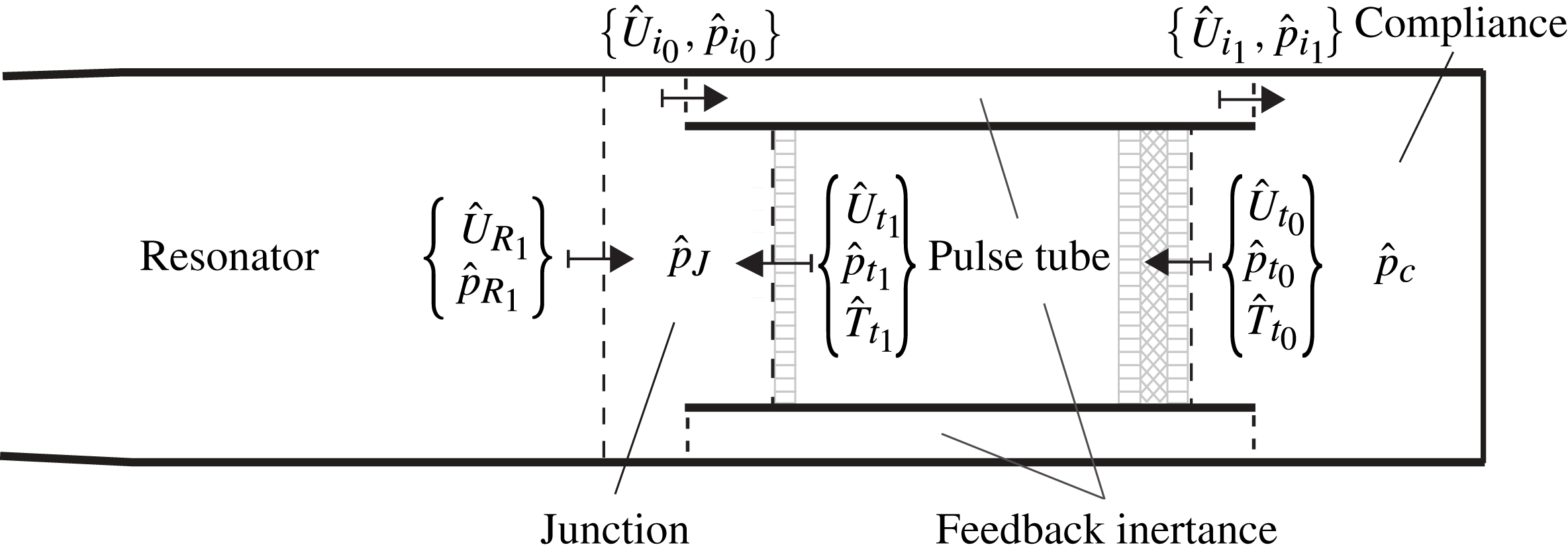
Building upon well-established linear modelling approaches (Rott Reference Rott1969; Ward & Swift Reference Ward and Swift1994; de Waele Reference de Waele2009), the engine is divided into a collection of control volumes (figure 8), representing different components, each modelled as a one- or zero-dimensional element, exchanging acoustic power and mass with adjacent components. Data from the Navier–Stokes simulations suggests that the pressure field is uniform within the compliance, consistent with de Waele (Reference de Waele2009)’s modelling choices. Such a component is, in fact, compact with respect to the fundamental wavelength. By imposing the conservation of mass and assuming an isentropic relation between volume-averaged density and pressure variations one obtains, in the time domain,
 $$\begin{eqnarray}\frac{\text{d}}{\text{d}t}p_{c}^{\prime }=w_{c_{0}}[U_{i_{1}}^{\prime }-U_{t_{0}}^{\prime }],\end{eqnarray}$$
where
 $p_{c}^{\prime }$
,
 $U_{i_{1}}^{\prime }$
and
 $U_{t_{0}}^{\prime }$
are, respectively, the instantaneous fluctuating pressure in the compliance and flow rates exchanged with the inertance through surface
 $i_{1}$
, and with the pulse tube through
 $t_{0}$
(figure 8), and
 $w_{c_{0}}={\it\gamma}P_{0}/V_{c_{0}}$
, where
 $P_{0}$
is the base pressure and
 $V_{c_{0}}$
the volume of the compliance.
Sketch illustrating the subdivision of the engine into control volumes representing different components (cf. figure 1): compliance (c), pulse tube (t), feedback inertance (i), junction (J), and resonator (R). Control surfaces are shown with dashed lines marking the beginning (0) and the end (1) of one-dimensional segments (oriented according to arrows) modelling the pulse tube, inertance and resonator. Complex pressure, volumetric flow rate and temperature are indicated with
 $\hat{p}$
,
 $\hat{U}$
and
 $\hat{T}$
respectively. References to the TBT are dropped in the context of the analysis of the startup phase during which nonlinear effects can be neglected. The left end of the control volume representing the junction is located at
 $x=-23~\text{mm}$
.
The very small variation among the growth rates and frequencies extracted from the numerical simulations at the locations in figure 7 (not shown) suggests that normal modes can be assumed for all fluctuating quantities. By adopting the
 $\text{e}^{+\text{i}{\it\sigma}t}$
convention with
 ${\it\sigma}=-\text{i}{\it\alpha}+{\it\omega}$
, where
 ${\it\alpha}$
and
 ${\it\omega}$
are, respectively, the growth rate and the angular frequency, (4.21) becomes
 $$\begin{eqnarray}\text{i}{\it\sigma}\hat{p}_{c}=w_{c_{0}}[\hat{U} _{i_{1}}-\hat{U} _{t_{0}}].\end{eqnarray}$$
The same modelling approach is adopted for convenience at the junction, where the conservation of mass reads
 $$\begin{eqnarray}\text{i}{\it\sigma}\hat{p}_{J}=w_{J_{0}}[\hat{U} _{R_{1}}-\hat{U} _{i_{0}}+\hat{U} _{t_{1}}]\end{eqnarray}$$
with
 $w_{J_{0}}={\it\gamma}P_{0}/V_{J_{0}}$
, where
 $V_{J_{0}}$
is the volume of the control volume modelling the junction (figure 8).
Phase variations along the axial coordinate,
 $x$
, are significant for the other components of the engine and the direct application of the complete set of linearized Euler equations is necessary. In all cases, the fluctuating field and the base state, defined by
 ${\it\rho}_{0}$
,
 $T_{0}$
and
 $P_{0}$
, are assumed to be exclusively a function of
 $x$
.
For the resonator (R) and feedback inertance (
 $\text{i}$
) isentropic wave propagation is assumed, yielding a simplified set of linearized equations for mass and momentum,
 $$\begin{eqnarray}\displaystyle & \displaystyle \text{i}{\it\sigma}\hat{p}=-\frac{{\it\rho}_{0}a_{0}^{2}}{A(x)}\frac{\text{d}\hat{U} }{\text{d}x}, & \displaystyle\end{eqnarray}$$
 $$\begin{eqnarray}\displaystyle & \displaystyle \text{i}{\it\sigma}\hat{U} =-\frac{A(x)}{{\it\rho}_{0}}\frac{\text{d}\hat{p}}{\text{d}x}, & \displaystyle\end{eqnarray}$$
 $A(x)$
, where
 $a_{0}=\sqrt{{\it\gamma}RT_{0}}$
is the speed of sound based on the base temperature. By introducing a spatial discretization, the set of equations (4.24) can be recast in algebraic form, as
 $$\begin{eqnarray}(\text{i}{\it\sigma}\unicode[STIX]{x1D644}-\boldsymbol{B}_{R})\boldsymbol{\cdot }\boldsymbol{u}_{R}=0\end{eqnarray}$$
for the resonator, and
 $$\begin{eqnarray}(\text{i}{\it\sigma}\unicode[STIX]{x1D644}-\boldsymbol{B}_{i})\boldsymbol{\cdot }\boldsymbol{u}_{i}=0\end{eqnarray}$$
for the inertance, where
 $\unicode[STIX]{x1D644}$
is the identity matrix,
 $\boldsymbol{B}$
is an operator discretizing the right-hand side of (4.24), and
 $\boldsymbol{u}$
is a discrete collection of complex amplitudes for pressure and flow rate, specifically,
 $\boldsymbol{u}_{R}=\{\hat{\boldsymbol{p}}_{R},\hat{\boldsymbol{U}}_{R}\}$
for the resonator, and
 $\boldsymbol{u}_{i}=\{\hat{\boldsymbol{p}}_{i},\hat{\boldsymbol{U}}_{i}\}$
for the feedback inertance.
The systems of equations (4.25) and (4.26) are isolated component eigenvalue problems (with boundary conditions to be specified) and their resolution, in the context of a system-wide linear stability analysis, is only meaningful if coupled with all of the other components in the engine, as discussed in the following.
The heat transfer and drag in the pulse tube, and the presence of gradients of base density and temperature in the REG/HX unit, require variations of entropy to be explicitly accounted for. Replacing the conservation equation for the total energy with the transport equation for entropy, expressed in terms of temperature and pressure using Gibbs’ relation, yields
 $$\begin{eqnarray}\displaystyle & \displaystyle \text{i}{\it\sigma}A\hat{{\it\rho}}+\frac{\text{d}\hat{U} }{\text{d}x}{\it\rho}_{0}+\hat{U} \frac{\text{d}{\it\rho}_{0}}{\text{d}x}=0, & \displaystyle\end{eqnarray}$$
 $$\begin{eqnarray}\displaystyle & \displaystyle \text{i}{\it\sigma}\hat{U} +\frac{A}{{\it\rho}_{0}}\frac{\text{d}\hat{p}}{\text{d}x}=-\frac{R_{C}}{{\it\rho}_{0}}\hat{U} , & \displaystyle\end{eqnarray}$$
 $$\begin{eqnarray}\displaystyle & \displaystyle {\it\rho}_{0}C_{p}\left[\text{i}{\it\sigma}\hat{T}+\frac{\hat{U} }{A}\frac{\text{d}T_{0}}{\text{d}x}\right]-\text{i}{\it\sigma}\hat{p}=-{\it\alpha}_{T}\hat{T}, & \displaystyle\end{eqnarray}$$
 $t=0.55~\text{s}$
(figure 5
a), at the early stages of the startup phase (figure 4).
Recasting the system of equations in (4.27) in diagonalized form yields
 $$\begin{eqnarray}\displaystyle & \displaystyle \text{i}{\it\sigma}\hat{p}=\left[{\it\rho}_{0}R\mathscr{B}_{\hat{T}\hat{U} }-\frac{P_{0}}{A}\frac{\text{d}}{\text{d}x}-\frac{RT_{0}}{A}\frac{\text{d}{\it\rho}_{0}}{\text{d}x}\right]\hat{U} +[{\it\rho}_{0}R\mathscr{B}_{\hat{T}\hat{T}}]\hat{T}, & \displaystyle\end{eqnarray}$$
 $$\begin{eqnarray}\displaystyle & \displaystyle \text{i}{\it\sigma}\hat{U} =\left[-\frac{A}{{\it\rho}_{0}}\frac{\text{d}}{\text{d}x}\right]\hat{p}+\left[-\frac{R_{c}}{{\it\rho}_{0}}\right]\hat{U} , & \displaystyle\end{eqnarray}$$
 $$\begin{eqnarray}\displaystyle & \displaystyle \text{i}{\it\sigma}\hat{T}=\mathscr{B}_{\hat{T}\hat{U} }\hat{U} +\mathscr{B}_{\hat{T}\hat{T}}\hat{T}, & \displaystyle\end{eqnarray}$$
 $$\begin{eqnarray}\displaystyle & \displaystyle \mathscr{B}_{\hat{T}\hat{U} }=-\frac{T_{0}}{A}\left[\frac{1}{T_{0}}\frac{\text{d}T_{0}}{\text{d}x}+({\it\gamma}-1)\frac{\text{d}}{\text{d}x}\right], & \displaystyle\end{eqnarray}$$
 $$\begin{eqnarray}\displaystyle & \displaystyle \mathscr{B}_{\hat{T}\hat{T}}=-\frac{{\it\gamma}{\it\alpha}_{T}}{{\it\rho}_{0}C_{p}}, & \displaystyle\end{eqnarray}$$
 $$\begin{eqnarray}(\text{i}{\it\sigma}\unicode[STIX]{x1D644}-\boldsymbol{B}_{t})\boldsymbol{\cdot }\boldsymbol{u}_{t}=0,\end{eqnarray}$$
where
 $\boldsymbol{u}_{t}=\{\hat{\boldsymbol{p}}_{t},\hat{\boldsymbol{U}}_{t},\hat{\boldsymbol{T}}_{t}\}$
.
The complete eigenvalue problem can finally be solved by coupling the isolated component eigenvalue problems (4.22), (4.23), (4.25), (4.26) and (4.31) via the following conditions
 $$\begin{eqnarray}\displaystyle & \displaystyle \hat{U} _{R_{0}}=0, & \displaystyle\end{eqnarray}$$
 $$\begin{eqnarray}\displaystyle & \displaystyle \left.\frac{\text{d}}{\text{d}x}\hat{p}_{R}\right|_{0}=0, & \displaystyle\end{eqnarray}$$
 $$\begin{eqnarray}\displaystyle & \displaystyle \hat{p}_{J}=\hat{p}_{R_{1}}=\hat{p}_{i_{0}}=\hat{p}_{t_{1}}, & \displaystyle\end{eqnarray}$$
 $$\begin{eqnarray}\displaystyle & \displaystyle \hat{p}_{c}=\hat{p}_{i_{1}}=\hat{p}_{t_{0}}, & \displaystyle\end{eqnarray}$$
 $$\begin{eqnarray}\displaystyle & \displaystyle \hat{T}_{t_{1}}=\frac{1}{{\it\rho}_{0}R}\frac{{\it\gamma}-1}{{\it\gamma}}\hat{p}_{J}, & \displaystyle\end{eqnarray}$$
 $$\begin{eqnarray}\displaystyle & \displaystyle \hat{T}_{t_{0}}=\frac{1}{{\it\rho}_{0}R}\frac{{\it\gamma}-1}{{\it\gamma}}\hat{p}_{c}, & \displaystyle\end{eqnarray}$$

where
 $\boldsymbol{v}=\{\boldsymbol{u}_{t};\boldsymbol{u}_{R};\boldsymbol{u}_{i}\}$
, and then incorporating the conditions (4.32) and the equations (4.22) and (4.23) to close the problem. Each of the conditions in (4.32), (4.22) and (4.23) replaces one corresponding equation in (4.33), therefore, not affecting the rank of the system. The eigenvalue structure is finally recovered by absorbing the equations that do not contain
 ${\it\sigma}$
(i.e. the ones deriving from (4.32)) via Gaussian elimination.
The linear modelling framework composed of equations (4.22)–(4.24) and (4.27) is first tested against the three-dimensional numerical simulation data for verification purposes. First, the acoustic impedance at different axial positions in the resonator, obtained by numerically integrating (4.24), has been quantitatively verified against the simulation data, as well as the constants
 $w_{c_{0}}$
in (4.22) and
 $w_{J_{0}}$
in (4.23), which are equal to
 $135\times 10^{6}~\text{N}~\text{m}^{-5}$
and
 $312\times 10^{6}~\text{N}~\text{m}^{-5}$
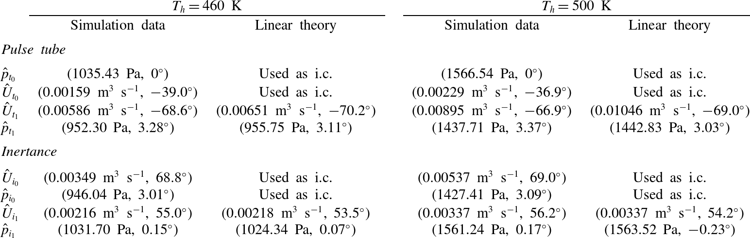
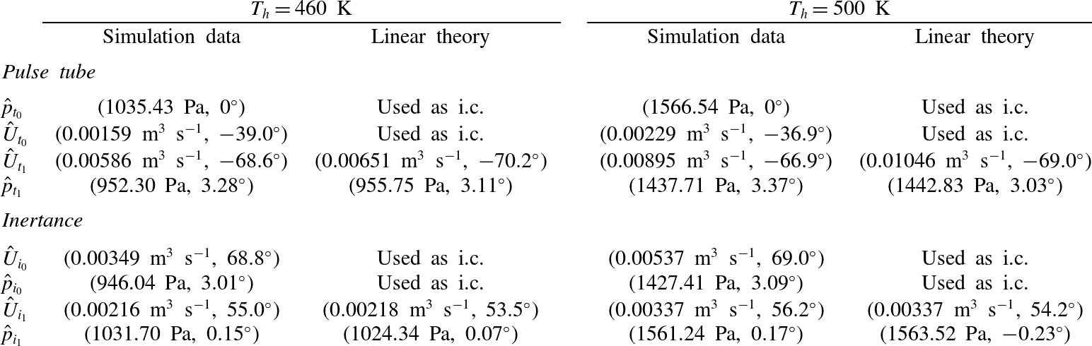
, respectively. Good agreement is also obtained by directly integrating (4.27) from section
 $t_{0}$
to
 $t_{1}$
and
 $i_{0}$
to
 $i_{1}$
(figure 8) using data from the numerical simulations as initial conditions (table 3). The integration has been carried out with the exact value of the frequency and growth rate extracted from the simulations (figure 9). Numerical trials have shown that, for a given initial condition and base state, the direct integration of (4.27) is much more sensitive to the angular frequency
 ${\it\omega}$
than the growth rate
 ${\it\alpha}$
, which suggests that the prediction of the latter, in thermoacoustic systems, is potentially problematic, especially within the framework of linear modelling in the spectral domain.
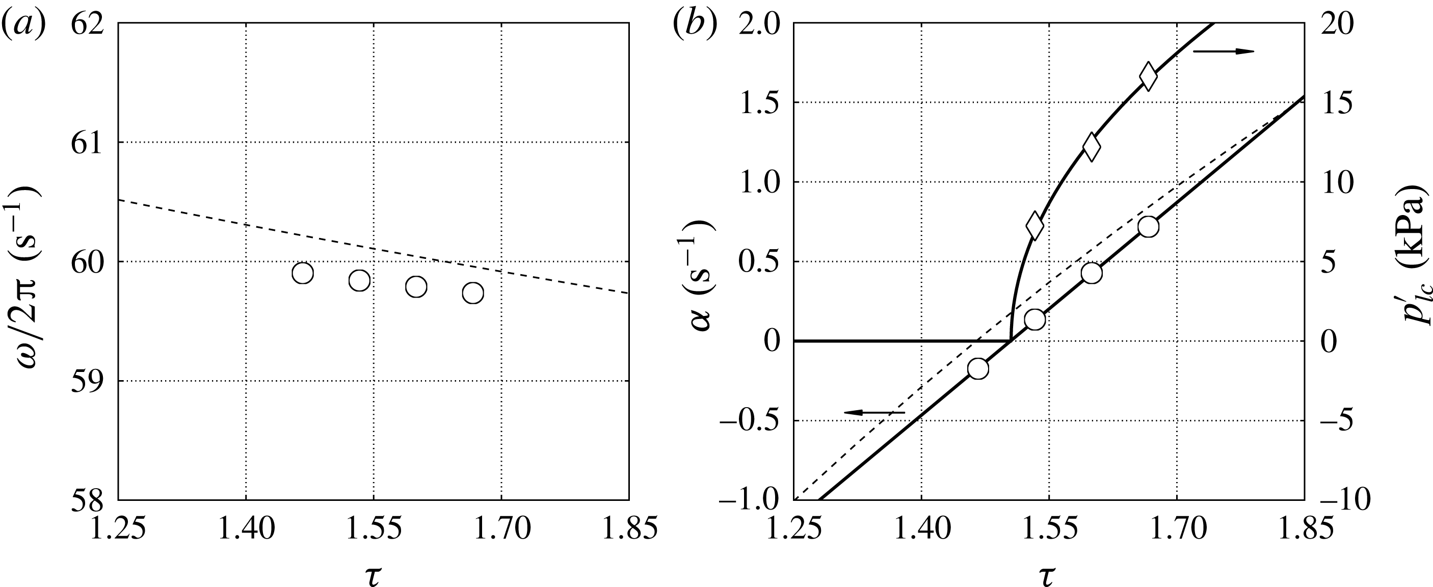
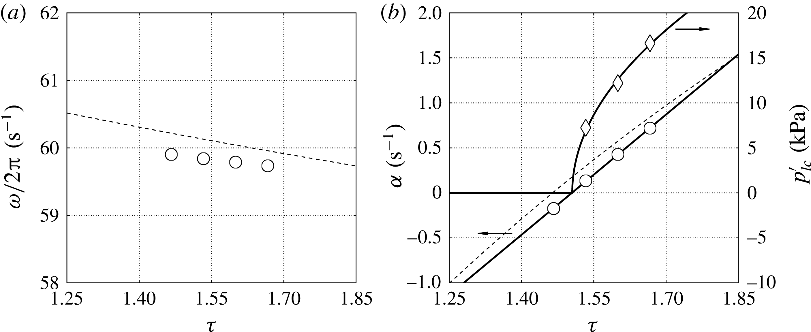
(a) Frequency,
 ${\it\omega}/2{\rm\pi}$
, and (b) growth rate,
 ${\it\alpha}$
, and limit-cycle pressure amplitude,
 $p_{lc}^{\prime }$
, versus hot-to-cold temperature ratio,
 ${\it\tau}=T_{h}/T_{c}$
. Linear stability model (- - -), numerical simulations (symbols) with corresponding fitting (—–) yielding the critical temperature ratio
 ${\it\tau}_{cr}=1.505$
and
 $\left.p_{lc}^{\prime }\right|_{{\it\delta}{\it\tau}=1}=41\,000~\text{Pa}$
.
Comparison between linear theory and simulation data for
 $T_{h}=460~\text{K}$
and
 $T_{h}=500~\text{K}$
extracted at locations shown in figure 8 at
 $t=0.55~\text{s}$
. The linearized equations (4.27) are integrated from
 $t_{0}$
to
 $t_{1}$
and
 $i_{0}$
to
 $i_{1}$
(figure 8) with initial conditions (i.c.) at
 $t_{0}$
and
 $i_{0}$
, respectively, and
 ${\it\alpha}$
,
 ${\it\omega}$
,
 $T_{0}(x)$
and
 ${\it\rho}_{0}(x)$
taken from the numerical simulations (figures 5
a, 9).
The eigenvalues
 ${\it\sigma}$
are finally calculated by directly solving the complete eigenvalue problem for operating conditions ranging between
 ${\it\tau}=1.25$
and
 ${\it\tau}=1.85$
, where
 ${\it\tau}=T_{h}/T_{c}$
is the hot-to-cold temperature ratio. The segments representing the pulse tube, inertance and resonator were discretized with 256, 64 and 32 points, respectively, with a fourth-order spatial polynomial reconstruction. The frequency of instability and its variation with
 ${\it\tau}$
are predicted within a
 ${\sim}0.2~\text{Hz}$
error (figure 9
a). The operating frequency of the system could also be predicted (with a
 ${\sim}1~\text{Hz}$
error) by simply solving the eigenvalue problem (4.24) in the complete variable-area resonator alone (without the pulse tube), in accordance with the phase distribution shown in figure 7(b), which is consistent with simple standing-wave resonance. The growth rate is slightly overpredicted (figure 9
b), having neglected viscous and nonlinear losses. Overall, the quantitative agreement is very encouraging, serving both as a verification step for the full Navier–Stokes calculations and to gain insight into the nature of the instability, also briefly discussed in the following section.
One could also think of solving the complete eigenvalue problem by iteratively integrating (4.27) and (4.28) in space, starting from a given set of initial conditions or guesses. This approach is adopted in DeltaEC (Ward & Swift Reference Ward and Swift1994) to predict the limit-cycle pressure and velocity distributions in TAEs, which is a valid approximation in the case of relatively low-pressure amplitudes, limited waveform distortion and simple geometries. Several numerical trials, however, have shown that applying the same approach to the eigenvalue problem above (valid for the startup phase only) leads to numerically unstable results, especially when trying to predict the growth rate. Accurately predicting the correct instability frequency, on the other hand, appears to be possible regardless of the quality of the specific strategy adopted. A fully implicit spatial formulation, similar to Helmholtz solvers used in investigations of thermoacoustically unstable reactive flows (Poinsot & Veynante Reference Poinsot and Veynante2011), which has been adopted in the present context, is the only one that has proved to be reliable.
4.4. Supercritical Hopf bifurcation
A linear fit of the growth rates,
 ${\it\alpha}$
, extracted from the numerical simulation data versus the temperature ratio
 ${\it\tau}=T_{h}/T_{c}$
(figure 9
b) suggests a critical value of
 ${\it\tau}_{cr}=1.505$
. This is in perfect agreement with the same value obtained by fitting the functional form suggested by the supercritical Hopf bifurcation model
 $$\begin{eqnarray}p_{lc}^{\prime }=\left.p_{lc}^{\prime }\right|_{{\it\delta}{\it\tau}=1}\sqrt{{\it\tau}-{\it\tau}_{cr}},\end{eqnarray}$$
to the limit-cycle pressure amplitudes
 $p_{lc}^{\prime }$
versus
 ${\it\tau}$
. A similar result is obtained via nonlinear modelling by Mariappan & Sujith (Reference Mariappan and Sujith2011). The fitting parameters in (4.34) are
 $\left.p_{lc}^{\prime }\right|_{{\it\delta}{\it\tau}=1}$
(dimensional) and
 ${\it\tau}_{cr}$
(dimensionless). Moreover, two assumptions required by the Hopf bifurcation theorem are also satisfied: the non-hyperbolicity condition,
 ${\it\alpha}=0$
and
 ${\it\omega}\neq 0$
at
 ${\it\tau}_{cr}$
(figure 9
a), and the transversality condition,
 $\text{d}{\it\alpha}/\text{d}{\it\tau}\neq 0$
at
 ${\it\tau}_{cr}$
(figure 9
b). These results have important implications on the parametrization of nonlinear fluxes, discussed later in § 5.2.
5. Nonlinear regime
The analysis carried out so far has been exclusively based on the assumption of linear acoustic perturbations and therefore limited to the startup phase. Nonlinear effects, however, are already detectable after only a few cycles of operation. These include the departure from exponential growth of the pressure amplitude (figure 4), the presence of broadband fine-scale flow structures associated with transitional turbulence, and a steady drift in the fluid parcels’ motion, already noticeable in the REG/HX during the startup phase (figure 5 b). The latter phenomenon is known as acoustic streaming, which is the focus on this section.
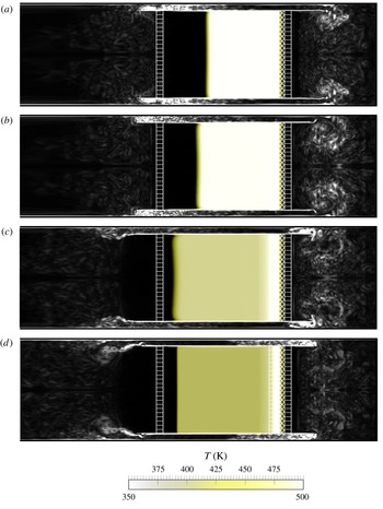
The most dramatic manifestation of acoustic streaming in travelling-wave TAEs is the advective heat leakage from the HHX (figure 10), which requires the introduction of the AHX2 (figure 1) to remove the excess heat and achieve a limit cycle. Acoustic streaming occurs everywhere in the engine, and its prediction and its suppression is one of the main technological challenges in the design of efficient TAEs.
Instantaneous visualizations of temperature contours (colourbar beneath) showing streaming of hot fluid in the TBT and vorticity magnitude (white) showing intense vortex shedding and transitional turbulence. Data is shown over one complete acoustic cycle with
 $90^{\circ }$
phase increments from (a) to (d). (See supplementary material available at http://dx.doi.org/10.1017/jfm.2014.745).

5.1. Direct modelling of acoustic streaming
A triple decomposition can be invoked to separate the streaming flow (rigorously defined below) from the acoustic field and the small-scale high-frequency fluctuations, starting with the Reynolds decomposition
 $$\begin{eqnarray}\displaystyle & {\it\rho}={\it\rho}_{0}+{\it\rho}^{\prime }, & \displaystyle\end{eqnarray}$$
 $$\begin{eqnarray}\displaystyle & p=p_{0}+p^{\prime }, & \displaystyle\end{eqnarray}$$
 $$\begin{eqnarray}\displaystyle & u_{i}=u_{0,i}+u^{\prime }, & \displaystyle\end{eqnarray}$$
 $$\begin{eqnarray}u_{0,i}=\overline{u}_{i}=\int _{-\infty }^{\infty }u_{i}(\boldsymbol{x},t+{\it\tau})\frac{\text{sin}({\rm\pi}f_{c}{\it\tau})}{{\rm\pi}{\it\tau}}\text{d}{\it\tau},\end{eqnarray}$$
where
 $f_{c}$
is the cutoff frequency. The filtering operation (5.2) is, in practice, carried out over six acoustic periods by adopting Simpson’s quadrature rule on the discrete data sampled at 2.2 kHz and
 $f_{c}=0.9f$
, where
 $f={\it\omega}/2{\rm\pi}$
is the acoustic frequency (figure 9
a). The remainder of the filtering operation in (5.1) can be further decomposed into a purely acoustic (subscript ‘
 $a$
’) and a small-scale component (subscript ‘
 $t$
’),
 $$\begin{eqnarray}\displaystyle & {\it\rho}^{\prime }={\it\rho}_{a}^{\prime }+{\it\rho}_{t}^{\prime }, & \displaystyle\end{eqnarray}$$
 $$\begin{eqnarray}\displaystyle & p^{\prime }=p_{a}^{\prime }+p_{t}^{\prime }, & \displaystyle\end{eqnarray}$$
 $$\begin{eqnarray}\displaystyle & u_{i}^{\prime }=u_{a,i}^{\prime }+u_{t,i}^{\prime }, & \displaystyle\end{eqnarray}$$
 $f$
while preserving the full acoustic amplitude. Due to the truncation in time of the filter kernel, this was achieved, in practice, with a cutoff frequency of
 $f_{c}>10f$
.
No evidence of significant turbulent activity has been found in the resonator. The Stokes Reynolds number in the neck is approximately 750, barely entering the intermittently turbulent regime (Jensen, Sumer & Fredsøe Reference Jensen, Sumer and Fredsøe1989). The low Stokes Reynolds number, together with other complex geometrical features, does not allow turbulence to be fully developed during the acoustic cycle.
Vorticity contours from instantaneous visualizations (figure 10) suggest that the most intense small-scale fluctuations occur in the feedback inertance. The unsteadiness of the (larger-scale) acoustic fluctuations does not allow turbulence to reach a fully (or even partially) developed state. The Reynolds number based on the Stokes thickness
 ${\it\delta}_{{\it\nu}}=\sqrt{2{\it\nu}/{\it\omega}}$
and the maximum velocity amplitude at the centre of the feedback inertance is approximately
 $Re_{{\it\delta}_{{\it\nu}}}=360$
(far below the upper limit of the disturbed laminar regime described in Jensen et al. (Reference Jensen, Sumer and Fredsøe1989)), suggesting that the turbulent kinetic energy generated from the breakup of the vortices rolling up from the edges of the annular tube is not sustained by the wall-induced shear. Moreover, turbulent stresses extracted for the
 $T_{h}=500~\text{K}$
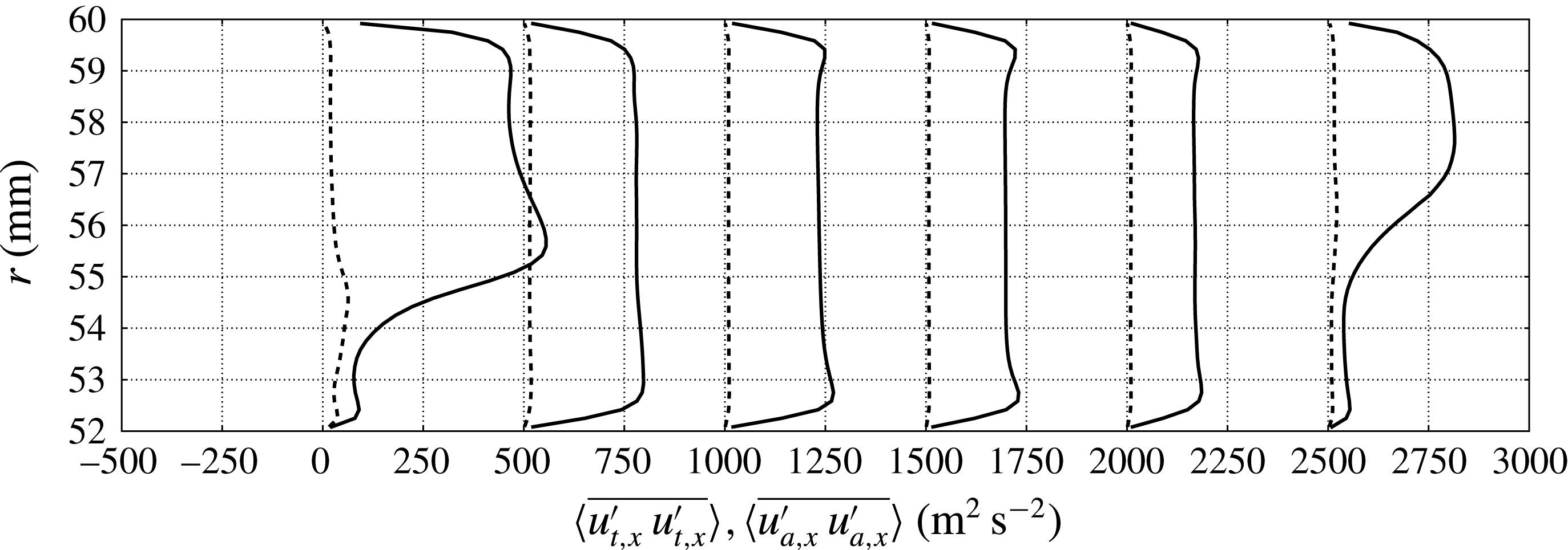
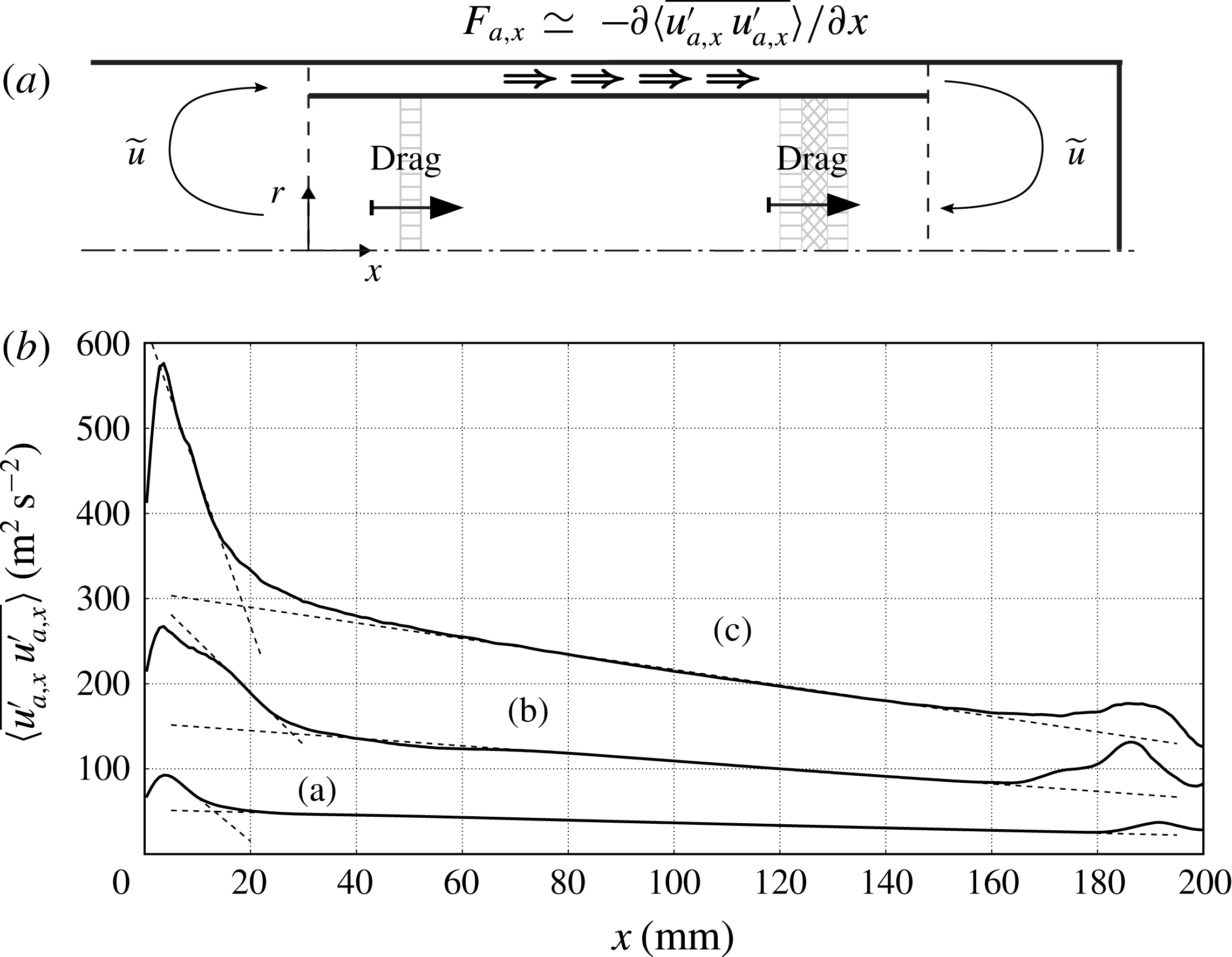
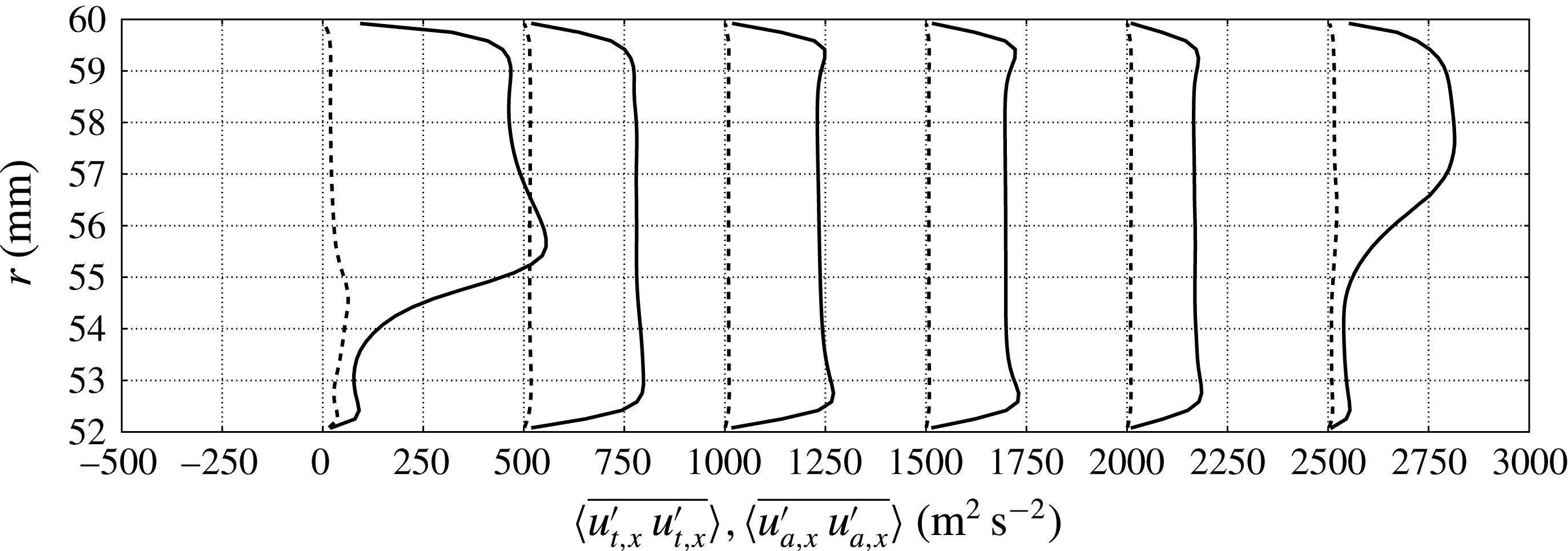
case (highest drive ratio) and for the finest grid available (table 2) are approximately two orders of magnitude smaller than the acoustic stresses (figure 11) and will be neglected in the following analysis. This choice also accommodates the need to devise a simple predictive modelling framework for the streaming velocity (5.7), which is discussed in the following.
Profiles of cycle- and time-averaged variance of acoustic
 $\langle \overline{u_{a,x}^{\prime }u_{a,x}^{\prime }}\rangle$
(—–) and small-scale
 $\langle \overline{u_{t,x}^{\prime }u_{t,x}^{\prime }}\rangle$
axial velocity fluctuations (– –) extracted in the inertance, for
 $x/L_{i}=0.01,0.2,0.40,0.60,0.80,0.99$
, from left to right, where
 $L_{i}=0.204~\text{m}$
(shifted by
 $500~\text{m}^{2}~\text{s}^{-2}$
for clarity) for
 $T_{h}=500~\text{K}$
and grid C (table 2).
Substituting the decomposition (5.1) into the time-filtered conservation of mass, ignoring temporal and spatial variations of the filtered density field (a strong assumption, particularly for the regions around the sharp edges and in the TBT), assuming that second-order quantities in the small-scale fluctuations are negligible with respect to their acoustic counterpart (figure 11),
 $$\begin{eqnarray}\displaystyle & \overline{u_{t,i}^{\prime }u_{t,i}^{\prime }}\ll \overline{u_{a,i}^{\prime }u_{a,i}^{\prime }}, & \displaystyle\end{eqnarray}$$
 $$\begin{eqnarray}\displaystyle & \overline{{\it\rho}_{t}^{\prime }u_{t,i}^{\prime }}\ll \overline{{\it\rho}_{a}^{\prime }u_{a,i}^{\prime }}, & \displaystyle\end{eqnarray}$$
 $$\begin{eqnarray}\frac{\partial \tilde{u} _{i}}{\partial x_{i}}=0,\end{eqnarray}$$
where
 $\tilde{u} _{i}$
is the density-weighted velocity field,
 $\tilde{u} _{i}=\overline{{\it\rho}u_{i}}/{\it\rho}_{0}$
, defined based on the filtering operation (5.2), which, under the assumptions made, can be expressed as
 $$\begin{eqnarray}\tilde{u} _{i}\simeq u_{0,i}+\frac{\overline{{\it\rho}_{a}^{\prime }u_{a_{i}}^{\prime }}}{{\it\rho}_{0}}.\end{eqnarray}$$
In the present manuscript the density-weighted velocity field,
 $\tilde{u} _{i}$
, is adopted as the definition of the streaming velocity based on (5.7), which is second-order accurate in wave amplitude.
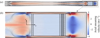
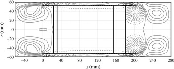
The streaming velocity field in our case is axially symmetric and spans the full extent of the engine (figure 12). Very large and elongated recirculations, of the order of a quarter of the acoustic wavelength, are visible in the resonator and are driven by the wall-normal gradient of the wave-induced shear stresses (not shown). Large recirculations of the order of the resonator radius near the sharp edges of the pulse tube and a mean flow circulating around the pulse tube (following the direction of the amplified waves) are also observed. The latter is called Gedeon (or DC) streaming (Gedeon Reference Gedeon1997) and is responsible for the mean transport of hot fluid away from the HHX, in the direction of the AHX2. As a result of such advective process, the TBT experiences a significant thermal load, with hot fluid occupying, on average, a significant portion of the TBT’s length at the limit cycle (figure 10). Such a process, leading to heat leakage, limits the efficiency of most travelling-wave TAEs, as also discussed later in the context of the present engine.
Contours of axial component of time-averaged streaming velocity
 $\langle \tilde{u} _{x}\rangle$
(5.7) for
 $T_{h}=500~\text{K}$
and grid C (table 2). Full-scale visualization (a) and zoom on the right end (b). Results have been mirrored about the centreline and streamlines have been only numerically approximated for illustrative purposes.

Assuming that time scales of variation of the filtered quantities
 ${\it\rho}_{0}$
and
 $u_{0,i}$
are much longer than the acoustic period, and under the same assumptions underlying the derivation of (5.7), it can be shown that
 $\tilde{u} _{i}$
satisfies the incompressible Navier–Stokes equations (Rudenko & Soluyan Reference Rudenko and Soluyan1977),
 $$\begin{eqnarray}\frac{\partial \tilde{u} _{i}}{\partial t}+\frac{\partial }{\partial x_{j}}\tilde{u} _{i}\tilde{u} _{j}+\frac{\partial p_{0}}{\partial x_{i}}-{\it\nu}{\rm\nabla}^{2}\tilde{u} _{i}=F_{a,i},\end{eqnarray}$$
where
 $p_{0}=P_{0}/{\it\rho}_{0}$
and the forcing term
 $F_{a,i}$
is the divergence of the wave-induced Reynolds stresses, which can be expressed to second-order accuracy in wave amplitude as
 $$\begin{eqnarray}F_{a,i}=-\frac{\partial }{\partial x_{j}}\overline{u_{a,j}^{\prime }u_{a,i}^{\prime }}+\frac{\partial }{\partial x_{j}}\left\{-\frac{{\it\nu}}{{\it\rho}_{0}}\left[\frac{\partial }{\partial x_{j}}\overline{{\it\rho}_{a}^{\prime }u_{a,i}^{\prime }}+\frac{\partial }{\partial x_{i}}\overline{{\it\rho}_{a}^{\prime }u_{a,j}^{\prime }}\right]+\frac{2}{3}\frac{{\it\nu}}{{\it\rho}_{0}}\frac{\partial }{\partial x_{k}}\overline{{\it\rho}_{a}^{\prime }u_{a,k}^{\prime }}{\it\delta}_{ij}\right\}.\end{eqnarray}$$
For large Reynolds numbers based on the streaming velocity, the terms containing the molecular diffusion in (5.9) can be neglected, finally yielding
 $$\begin{eqnarray}F_{a,i}\simeq -\frac{\partial }{\partial x_{j}}\overline{u_{a,j}^{\prime }u_{a,i}^{\prime }}.\end{eqnarray}$$
The maximum value of the stresses
 $\overline{u_{a,j}^{\prime }u_{a,i}^{\prime }}$
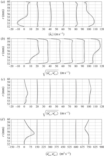
is expected to be found in the feedback inertance where the acoustic power is maximum in the system. A grid-sensitivity study on all of the components of the stresses in the inertance (figure 13) shows monotonic grid convergence of the stresses from grid A to C (table 2).
Profiles of time-averaged streaming velocity (a) and wave-induced Reynolds stresses (b–d) in the inertance, for
 $x/L_{i}=0.01,0.2,0.40,0.60,0.80,0.99$
, respectively from left to right, where
 $L_{i}=0.204~\text{m}$
(shifted by
 $20~\text{m}~\text{s}^{-1}$
or
 $150~\text{m}^{2}~\text{s}^{-2}$
for clarity). Data for
 $T_{h}=500~\text{K}$
and grid A (— ⋅ —), grid B (– –) and grid C (—–) (table 2). The time-averaged volumetric flux through the inertance (intensity of Gedeon streaming) for this drive ratio is approximately
 $0.0033~\text{m}^{3}~\text{s}^{-1}$
, corresponding to a mean streaming velocity of
 $1.2~\text{m}~\text{s}^{-1}$
.

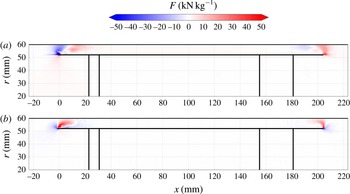
The direct evaluation of (5.10) from the numerical data reveals very high values of
 $F_{a,i}$
near the sharp edges of the annular tube (figure 14) which locally drive the large aforementioned recirculations. On the other hand, Gedeon streaming is driven by the viscous decay of the wave amplitude in the annular inertance. This results in a negative axial gradient of normal stress
 $\overline{u_{a,x}^{\prime }u_{a,x}^{\prime }}$
, visible in both figures 14 and 13(b).
Contour plots of the divergence of wave-induced Reynolds stresses. (a) Axial,
 $F_{a,x}$
, and (b) radial,
 $F_{a,r}$
, components extracted for
 $T_{h}=500~\text{K}$
on grid C (table 2).

An axially symmetric numerical model,
 $\text{Stream}^{\text{X}}$
(for more details see appendix A), has been developed to directly simulate the streaming velocity field as the solution of the incompressible equation (5.8) driven by the divergence of the wave-induced stresses (figure 14) extracted from the three-dimensional fully compressible calculations. Secondary features such as steady large-scale recirculations near the sharp edges of the annular tube are only qualitatively reproduced (figure 15), with the appearance of a second recirculation in the compliance, which is not observed in the calculations. The actual target of the present low-order modelling effort is the prediction of the intensity of the Gedeon streaming. In spite of the numerical challenges involved in solving incompressible flow in the presence of a sharp edge, the latter is predicted fairly accurately (figure 17
a), especially for low drive ratios. For high drive ratios, resulting in very high limit-cycle acoustic amplitudes, the errors associated with the assumptions made in deriving (5.7), (5.8) and (5.10) become too severe. ‘Slow’ streaming (Rudenko & Soluyan Reference Rudenko and Soluyan1977) never actually occurs in our engine, where the maximum intensity of
 $\tilde{u}$
is comparable to the acoustic velocity amplitude in all cases.
Positive (—–) and negative (– –) iso-levels of the Stokes streamfunction from the incompressible solver
 $\text{Stream}^{\text{X}}$
driven by the wave-induced Reynolds stresses (figure 14) extracted from the fully compressible three-dimensional calculations for
 $T_{h}=500~\text{K}$
on grid C (table 2).

5.2. Efficiency and energy fluxes in the TBT
As the acoustic energy grows during the initial transient, so does the intensity of the Gedeon streaming, increasing the rate of advective transport of hot fluid away from the HHX towards the AHX2. This results in unwanted heat leakage, which lowers the overall energy conversion efficiency. The gradual expansion of the gas in the TBT determines a slow increase of the background pressure in the system (not shown), which plateaus only when the hot temperature front enters into contact with the AHX2. At this point, a rapid increase of the growth rate is also observed, as shown by the kink in the time series in figure 4. This is due to a change in the structure of the velocity field in the TBT after the first contact between the hot gas front and the AHX2 occurs. As shown in figure 10, and in time series of instantaneous axial velocity in the TBT (not shown), when the hot gas is displaced towards the AHX2, the hot flow front is abruptly stopped by the sudden density increase caused by the cooling in the AHX2. This results in a reduction of the cycle-averaged velocity and, therefore, a temporary containment of the intensity of the Gedeon streaming and heat leakage from the HHX.
A limit cycle is only reached later, with a constant background pressure, when the losses in the system balance the enhanced acoustic energy production. These losses include streaming in the resonator and dissipation associated with the turbulent vortex shedding from the pulse tube walls.
The exact conservation equation for the density-averaged internal energy,
 $\tilde{e}=\overline{{\it\rho}e}/\overline{{\it\rho}}$
, reads (Lele Reference Lele1994)
 $$\begin{eqnarray}\frac{\partial }{\partial t}(\overline{{\it\rho}}\tilde{e})=-\frac{\partial }{\partial x_{j}}\left(\overline{{\it\rho}}\left[\tilde{u} _{j}\tilde{e}+\widetilde{h^{\prime \prime }u_{j}^{\prime \prime }}\right]-\overline{q}_{j}\right)+\frac{\partial }{\partial x_{j}}\left(\overline{p^{\prime }u_{j}^{\prime \prime }}\right)+\overline{u_{i}^{\prime \prime }}\frac{\partial \overline{p}}{\partial x_{i}}-\overline{p^{\prime }\frac{\partial u_{i}^{\prime \prime }}{\partial x_{i}}},\end{eqnarray}$$
where
 $u_{j}^{\prime \prime }=u_{i}-\tilde{u} _{i}$
and
 $h^{\prime \prime }=h_{i}-\tilde{h}$
are the fluctuations of the density-weighted averages of velocity and enthalpy, and
 $\overline{q}_{j}$
is the time-filtered molecular heat flux. Applying (5.11) to the flow in the TBT approximated as quasi one-dimensional, neglecting small terms and assuming equilibrium conditions, yields
 $$\begin{eqnarray}\underbrace{\langle \,\overline{{\it\rho}}\tilde{u} \tilde{e}\rangle }_{\text{Advective H.T.}}+\underbrace{\left\langle \,\overline{{\it\rho}}\widetilde{h^{\prime \prime }u^{\prime \prime }}\right\rangle }_{\text{Thermoacoustic H.T.}}-\underbrace{\left\langle \,\overline{p^{\prime }u^{\prime \prime }}\right\rangle }_{\text{Acoustic energy flux}}\simeq \text{const.},\end{eqnarray}$$
which is verified with fairly good approximation in the simulations (figure 16 b). The intensity of the advective heat transport in the TBT is proportional to the mean temperature profile, since the streaming velocity is uniform in this region (figure 12). The adjustment length back to ambient temperature of the mean temperature distribution increases with the drive ratio (figure 16 a). This is due to thermoacoustic heat transport mechanisms. As the hot fluid front is transported with stronger intensity towards the AHX2 by the high-amplitude velocity fluctuations, steeper instantaneous temperature gradients form at the interface between the AHX2 and the TBT (figure 10). The result is a net cycle-average conductive heat flux in the positive axial direction, creating a temperature buffer region. The intensity of the conductive heat flux in (5.11) is, however, negligible compared to the quantities in (5.12), which dominate the energy transport budget in the TBT.
(a) Axial distribution of mean temperature for
 $T_{h}=460~\text{K}$
,
 $T_{h}=480~\text{K}$
and
 $T_{h}=500~\text{K}$
and (b) surface integrated energy fluxes in (5.12) for grid C and
 $T_{h}=500~\text{K}$
at limit cycle. Acoustic power (- -), thermoacoustic heat transport, (– –), advective heat transport (— ⋅ —) and overall sum (○).
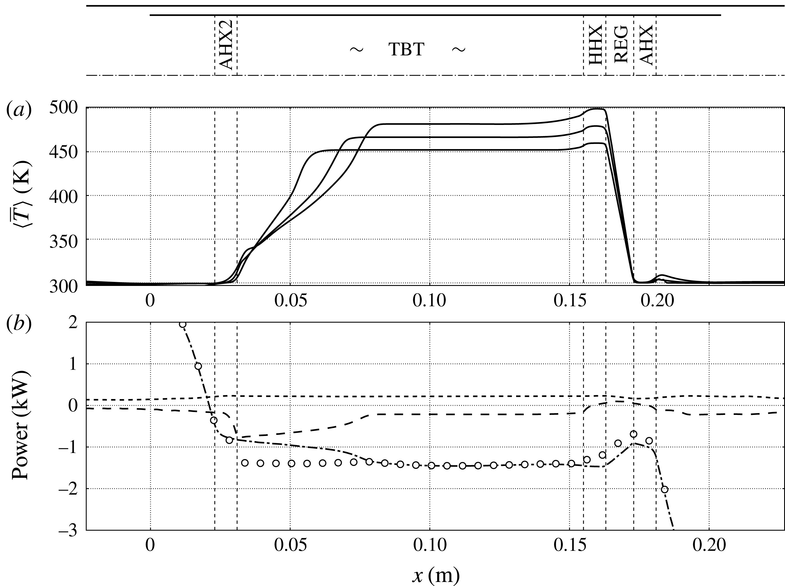
An accurate evaluation of the other terms in (5.11) is, unfortunately, made impractical by the (necessary) application of a second-order ENO reconstruction in the TBT and the smoothing associated with azimuthally averaging the three-dimensional unstructured data. The energy balance expressed by (5.12) is, however, satisfied to a sufficient degree of accuracy to gain insight into the role of the Gedeon streaming in determining the overall efficiency of the device and the scaling of the energy fluxes in (5.12).
While no direct energy extraction component (e.g. an acoustic load such as a piezo electric element or a linear alternator) has been included in the set-up investigated, a metric for efficiency can still be defined as
 $$\begin{eqnarray}{\it\eta}_{H}=\frac{\left\langle \,\overline{p^{\prime }u^{\prime \prime }}\right\rangle }{\left\langle \,\overline{{\it\rho}}\widetilde{h^{\prime \prime }u^{\prime \prime }}\right\rangle +\langle \,\overline{{\it\rho}}\tilde{u} \tilde{e}\rangle },\end{eqnarray}$$
which is the ratio between acoustic energy produced and total heat dissipated by the AHX2. For example, our theoretical device produces
 ${\sim}0.2~\text{kW}$
of acoustic power at
 $T_{h}=500~\text{K}$
while losing
 ${\sim}2.0~\text{kW}$
, mostly due to mean advection caused by Gedeon streaming, achieving a modest efficiency (
 ${\sim}10\,\%$
). Realistic travelling-wave TAEs can reach overall efficiencies of
 ${>}20\,\%$
, or even
 ${>}30\,\%$
if built in a cascaded configuration (Gardner & Swift Reference Gardner and Swift2003). The efficiency directly evaluated from the simulation data (figure 17
a) decreases rapidly with the temperature ratio, which could be expected in TAEs with excessive Gedeon streaming controlling the energy balance in the TBT (G.W. Swift, Personal communication, 2014). However, the uncertainties in the integral quantities in figure 17
b, due to averaging over a limited number (approximately 25) of acoustic cycles, makes the direct metric for the efficiency (5.13) not very reliable.
(a) Intensity of Gedeon streaming versus hot-to-cold temperature ratio for fully compressible Navier–Stokes simulations (▫) with corresponding fit (——), incompressible model (▪), order-of-magnitude analysis (5.16) (▹), efficiency
 ${\it\eta}_{H}$
(5.13) (


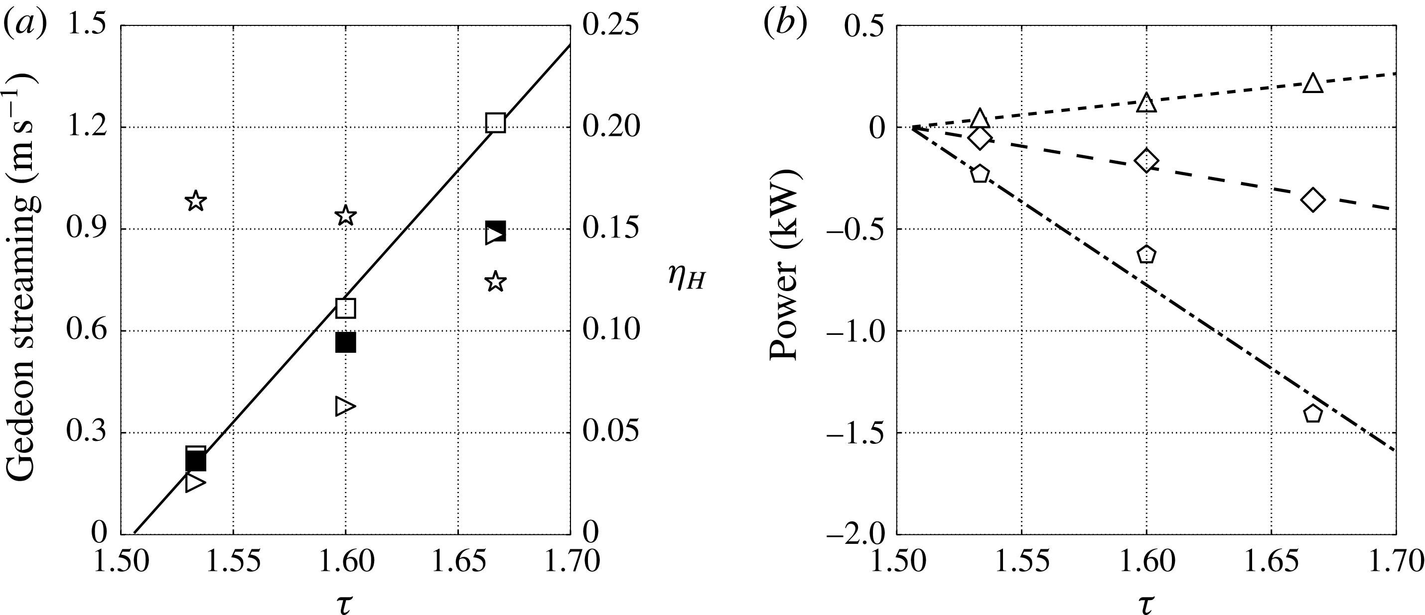
(a) Illustration of balance (5.16) between travelling-wave decay in feedback inertance and drag due to HXs and REG. (b) Streamwise profile of axial wave-induced stresses extracted at
 $r=56~\text{mm}$
for
 $T_{h}=460~\text{K}$
(a),
 $T_{h}=480~\text{K}$
(b) and
 $T_{h}=500~\text{K}$
(c) with linear fitting (- - -) approximating the mean decay rate.
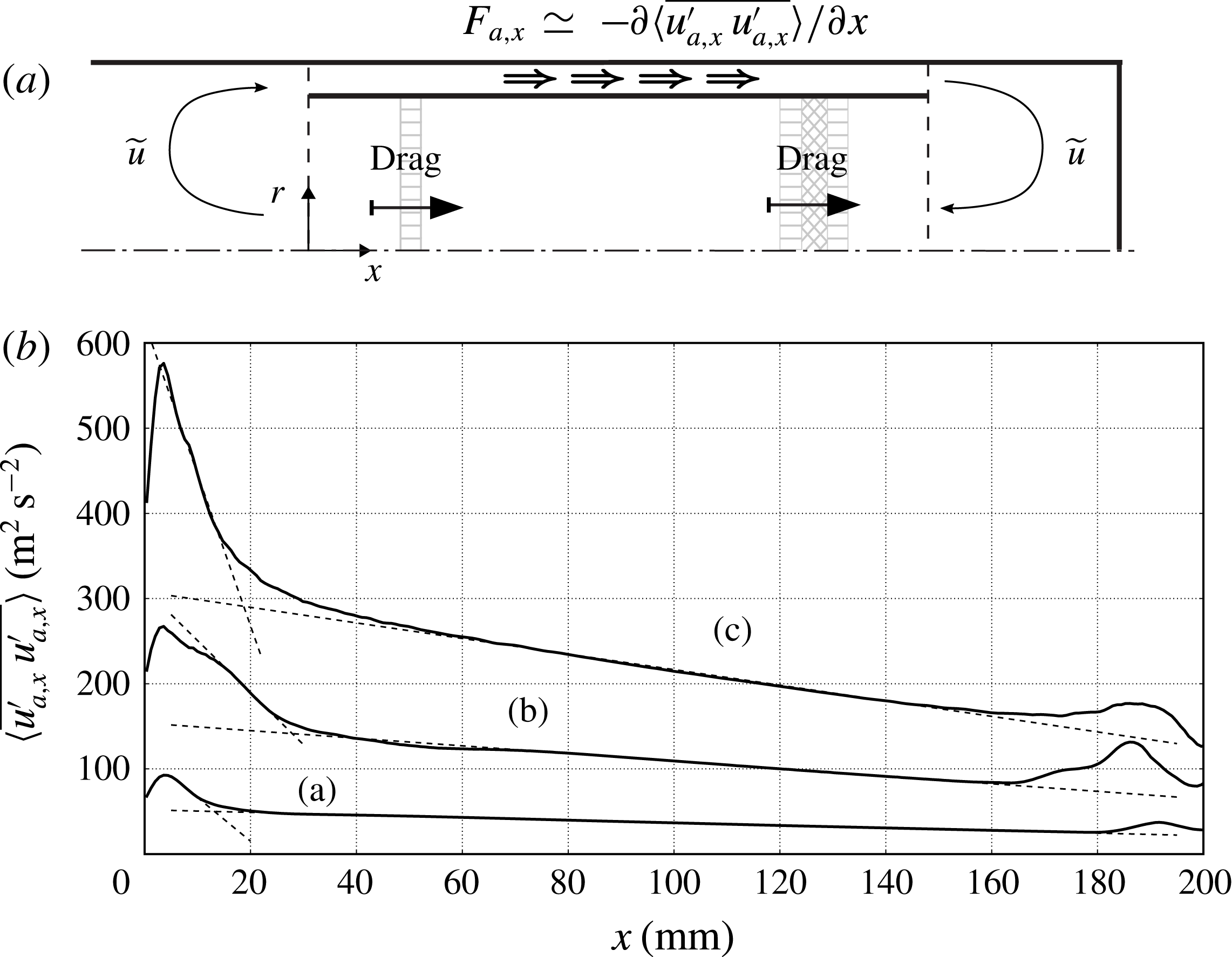
A more robust estimate for
 ${\it\eta}_{H}$
can be derived by investigating the scaling of the volume-averaged energy fluxes in (5.12) (figure 17
b) with a simple order-of-magnitude analysis and curve fitting. The advective flux in the TBT, driven by the Gedeon streaming, is expected to scale as
 $$\begin{eqnarray}\langle \overline{{\it\rho}}\tilde{u} \tilde{e}\rangle \sim {\it\rho}_{0,tbt}u_{dc}C_{v}T_{h},\end{eqnarray}$$
where
 ${\it\rho}_{0,tbt}\sim p_{0}/(RT_{c}{\it\tau})$
is the average density in the TBT and the hot temperature is simply
 $T_{h}=T_{c}{\it\tau}$
. The analytical expression of the streaming velocity due to a freely propagating travelling wave,
 $$\begin{eqnarray}u_{dc}=\frac{1}{2}\frac{|u_{lc}^{\prime }|^{2}}{a_{0}},\end{eqnarray}$$
suggests that the intensity of the streaming velocity scales quadratically with the limit-cycle velocity amplitude
 $u_{lc}^{\prime }\sim p_{lc}^{\prime }/({\it\rho}_{0}a_{0})$
. While the quadratic scaling of the streaming velocity is an expected result, a more quantitative estimate for
 $u_{dc}$
can be obtained by further simplifying the analysis in § 5.1, where the streaming velocity is directly modelled based on an hydrodynamic analogy. In fact, by roughly measuring the average spatial decay rate of the axial acoustic stresses in the inertance,
 $\langle F_{a,x}\rangle _{i}$
(figure 18
a), and equating that to the linearized viscous losses in the pulse tube (see (2.3a
)), the intensity of the Gedeon streaming can be estimated as
 $$\begin{eqnarray}u_{dc}\sim \frac{{\it\rho}_{0}A_{i}L_{i}\langle F_{a,x}\rangle _{i}}{V_{\mathit{AHX2}}R_{c,\mathit{AHX2}}+V_{\mathit{HHX}}R_{c,\mathit{HHX}}+V_{\mathit{REG}}R_{c,\mathit{REG}}+V_{\mathit{AHX}}R_{c,\mathit{AHX}}},\end{eqnarray}$$
where
 $V$
and
 $R_{c}$
are, respectively, the volume and drag coefficients (obtained by linearizing (2.3)) of the REG/HX unit in the pulse tube. The estimate (5.16) is in good quantitative agreement with the results from § 5.1 (figure 17
a), showing that, in this case, the viscous wave-amplitude decay in the inertance, leading to the generation of strong divergence of wave-induced Reynolds stresses, dominates over mean pressure gradient (
 $\partial p_{0}/\partial x_{i}$
in (5.8)) effects. The case for
 $T_{h}=480~\text{K}$
is an outlier simply due to the lack of grid convergence of the acoustic stresses for this particular case (table 2). The quadratic scaling adopted in (5.15) is, therefore, further justified by (5.16), where
 $\langle F_{a,x}\rangle _{i}\sim {u_{lc}^{\prime }}^{2}$
. By invoking the previously derived scaling for the limit-cycle pressure (4.34), (5.15) becomes
 $$\begin{eqnarray}u_{dc}=A_{dc}\frac{1}{2}\frac{1}{{\it\rho}_{0}^{2}a_{0}^{3}}\left.{p_{lc}^{\prime }}^{2}\right|_{{\it\delta}{\it\tau}=1}({\it\tau}-{\it\tau}_{cr}),\end{eqnarray}$$
where the fitting coefficient is
 $A_{dc}=0.52$
(figure 17
b). Substituting (5.17) into (5.14) yields
 $$\begin{eqnarray}\langle \,\overline{{\it\rho}}\tilde{u} \tilde{e}\rangle =A_{adv}\left[\frac{C_{v}P_{0}}{R}A_{dc}\frac{1}{2}\frac{1}{{\it\rho}_{0}^{2}a_{0}^{3}}\left.{p_{lc}^{\prime }}^{2}\right|_{{\it\delta}{\it\tau}=1}\right]({\it\tau}-{\it\tau}_{cr}),\end{eqnarray}$$
where the fitting coefficient is
 $A_{adv}=0.51$
. The same procedure can be applied to the acoustic energy flux, which scales as
 $$\begin{eqnarray}\langle \,\overline{p^{\prime }u^{\prime \prime }}\rangle \sim p_{lc}^{\prime }u_{lc}^{\prime }{\textstyle \frac{1}{2}}\,\text{cos}({\rm\Delta}{\it\phi}),\end{eqnarray}$$
where
 ${\rm\Delta}{\it\phi}$
is the phase difference between pressure and velocity observed in the REG/HX (figure 5
c), leading to
 $$\begin{eqnarray}\langle \,\overline{p^{\prime }u^{\prime \prime }}\rangle =A_{ap}\frac{1}{2}\,\text{cos}({\rm\Delta}{\it\phi})\frac{1}{{\it\rho}_{0}a_{0}}\left.{p_{lc}^{\prime }}^{2}\right|_{{\it\delta}{\it\tau}=1}({\it\tau}-{\it\tau}_{cr}),\end{eqnarray}$$
where the fitting constant is
 $A_{ap}=0.3$
. Finally, the thermoacoustic heat flux is expected to scale as
 $$\begin{eqnarray}\langle \,\overline{{\it\rho}}\widetilde{h^{\prime \prime }u^{\prime \prime }}\rangle \sim {\it\rho}_{0,tbt}C_{p}\frac{\partial T}{\partial P}p_{lc}^{\prime }\frac{p_{lc}^{\prime }}{{\it\rho}_{0}a_{0}}\frac{1}{2}\,\text{cos}({\rm\Delta}{\it\phi}),\end{eqnarray}$$
where
 ${\rm\Delta}{\it\phi}$
is needed to account for the correlation between pressure and velocity (like in (5.19)), resulting in
 $$\begin{eqnarray}\langle \,\overline{{\it\rho}}\widetilde{h^{\prime \prime }u^{\prime \prime }}\rangle =A_{ta}\left[\frac{1}{2{\it\rho}_{0}a_{0}}\left.{p_{lc}^{\prime }}^{2}\right|_{{\it\delta}{\it\tau}=1}\frac{1}{2}\,\text{cos}({\rm\Delta}{\it\phi})\right]({\it\tau}-{\it\tau}_{cr})\end{eqnarray}$$
with the fitting coefficient
 $A_{ta}=0.93$
. With all fluxes scaling as
 ${\sim}({\it\tau}-{\it\tau}_{cr})$
, this leads to a robust estimate for the efficiency,
 $$\begin{eqnarray}{\it\eta}_{H,\mathit{avrg}}=0.13,\end{eqnarray}$$
effectively averaged over the range of temperature ratios investigated.
Linear acoustic solvers applied at the limit cycle can directly estimate second-order quantities in the acoustic amplitudes such as (5.19) and (5.22), or even the mean wave-amplitude decay
 $\langle F_{a,x}\rangle _{i}$
due to viscous losses in a duct, without prior knowledge of the critical temperature ratio,
 ${\it\tau}_{cr}$
. However, process-based parametrizations for the Gedeon streaming, and therefore the advective transport (5.18), are still currently missing despite having a first-order impact on the acoustic energy budgets and the efficiency. We have shown that, for slow streaming, commonly found in realistic travelling-wave TAEs, a hydrodynamic analogy (Lighthill Reference Lighthill1978) can be invoked, and further simplified, leading to a very low-order modelling approach (5.16), which is very amenable in the context of simple linear solvers used for engineering prediction of TAEs. Moreover, estimates such as (5.16) do not require the knowledge of the critical temperature ratio
 ${\it\tau}_{cr}$
, making the hydrodynamic analogy investigated in § 5.1 an attractive modelling paradigm for streaming.
6. Conclusions
We have carried out three-dimensional numerical simulations of a theoretical travelling-wave TAE. This is the first step in a broader research effort aimed at building multi-fidelity, full-scale prediction tools for TAEs. The goal is to assist technological design by directly simulating, under realistic operating conditions, the physical processes controlling the overall efficiency of such devices. These include the thermoacoustic instability, wave propagation and amplification in the startup phase, the nonlinear effects at the limit cycle (mainly acoustic streaming and turbulence) and the effects of geometrical complexities. The last two are not directly captured in state-of-the-art predictive tools for TAEs.
Inspired by the work of Lycklama à Nijeholt et al. (Reference Lycklama à Nijeholt, Tijani and Spoelstra2005), we have devised a simple travelling-wave TAE model that could serve as a benchmark case for high-fidelity numerical simulations of similar devices. We have extended such a set-up to three dimensions and introduced a secondary AHX2 to achieve a limit cycle, modelling typical fluid dynamic conditions found in TBT. Details omitted in Lycklama à Nijeholt et al. (Reference Lycklama à Nijeholt, Tijani and Spoelstra2005) regarding the geometry and the modelling of the HXs and REGs have been reconstructed to the best of the authors’ ability and reported in detail. While the simplicity of the adopted REG/HX heat-transfer and drag models allows the straightforward development of companion linear and nonlinear models (necessary for verification of the Navier–Stokes calculations), other important processes typically occurring in the REG/HX unit are, inevitably, not directly simulated. In the linear regime, for example, the natural phase shift present between the instantaneous heat flux at the wall and gas temperature is not captured, since the adopted heat-transfer model assumes perfect thermal contact. Moreover, the mean hot (
 $T_{h}$
) and ambient (
 $T_{a}$
) temperatures are directly imposed in the calculations, not allowing one to capture, for example, the non-zero time-averaged temperature difference between gas and the HX metal observed in experiments in the nonlinear regime (Swift Reference Swift1992). Dissipation mechanisms due to vortex shedding at the scale of the pore or stack size of the REG, or hydrodynamic/thermal entrance effects are also not directly reproduced, while their effects are accounted for. Overall, in spite of the low-fidelity approach adopted in the REG/HX area, the complete computational model has proved to successfully reproduce the essential critical issues, features and complexities of real travelling-wave TAEs.
The time integration is carried out from initial quiescent conditions to the limit cycle. It is shown that the mechanisms responsible for the acoustic energy generation and propagation in the system during the startup phase can be explained with linear acoustics, despite the high amplitude (
 ${\sim}1\,\%$
of the mean) of the initial perturbation resulting from the activation of the source terms modelling the heat transfer. An analytical linear Lagrangian model shows that the thermoacoustic instability occurring in the REG/HX unit intensifies plane waves travelling in the direction of the imposed temperature gradient via a process resembling a thermodynamic Stirling cycle. The result is the establishment of a network of self-amplifying travelling waves looping around the REG/HX unit. A system-wide linear stability model based on Rott’s theory accurately predicts the frequency of the (only) unstable mode as well as the critical temperature ratio, despite not accounting for viscous and other nonlinear losses. The dependency of growth rates and limit-cycle pressure amplitudes on the temperature ratio are shown to be consistent with a supercritical Hopf bifurcation model. No evidence has been found to support subcritical or non-modal instability arguments.
At the limit cycle acoustic amplitudes exceed
 $+$
170 dB and nonlinear effects dominate the flow field in the form of transitional turbulence and acoustic streaming. The latter is the occurrence of a quasi-steady flow evolving over time scales much longer than the period of the waves inducing it. The data from the full three-dimensional simulations has allowed identification of the governing processes driving the streaming flow, which are viscous wave amplitude decay in the feedback inertance, periodic vortex ring rollup and breakup around the sharp edges of the annular tube, and near-wall acoustic shear stresses in the variable-area resonator. The strong influence of geometrical features on the structure of the streaming flow provides an effective means of controlling the latter, for example, by simple profiling of the TBT (Olson & Swift Reference Olson and Swift1997).
An axially symmetric numerical model based on the Stokes-streamfunction formulation has been adopted to directly simulate the streaming flow as the solution of the incompressible Navier–Stokes equations driven by the divergence of the wave-induced Reynolds stresses extracted from the fully compressible three-dimensional calculations. The model correctly reproduces the streaming flow patterns and, in spite of the strong assumptions made and numerical issues associated with geometric singularities, it correctly predicts the intensity of the Gedeon streaming. The latter is responsible for the decrease of the engine’s efficiency as the drive ratio is increased, and a robust parametrization for it is warranted. The investigation of the scaling of nonlinear fluxes reveals the importance of prior knowledge of the critical temperature ratio, which may not be straightforwardly achieved by simply relying on linear theory, for more complex systems.
Acknowledgements
The authors acknowledge the support of the Precourt Institute for Energy Seed Grant at Stanford and the computational time provided by the NSF-MRI grant on the Stanford Certainty cluster. The authors thank Dr G. Swift for his very useful comments on the draft and acknowledge the help of Professor R. Hixon for assisting in the development of the source terms to model the heat transfer and drag in heat exchanger and regenerators. C.S. would like to thank, in particular, Dr J. Bodart and Dr I. Bermejo-Moreno for their valuable technical help and Jeffrey Lin for providing the authors with a complete DeltaEC model of the engine, which has led to the choice of introducing a secondary ambient heat exchanger. The authors also thank the reviewers for their very useful comments, most of which have been incorporated in the present version of the manuscript.
Supplementary data
Supplementary data is available at http://dx.doi.org/10.1017/jfm.2014.745.
Appendix A.
 $\mathbf{Stream}^{\mathbf{X}}$
: an axially symmetric incompressible flow solver model

 $\text{Stream}^{\text{X}}$
solves the incompressible Navier–Stokes equations in cylindrical coordinates,
 $$\begin{eqnarray}\displaystyle & \displaystyle \frac{\partial u_{x}}{\partial t}+\frac{1}{r}\frac{\partial }{\partial r}(ru_{r}u_{x})+\frac{\partial }{\partial x}u_{x}^{2}=-\frac{\partial p}{\partial x}+{\it\nu}\left[\frac{1}{r}\frac{\partial }{\partial r}\left(r\frac{\partial u_{x}}{\partial r}\right)+\frac{\partial ^{2}u_{x}}{\partial x^{2}}\right]+F_{x}, & \displaystyle\end{eqnarray}$$
 $$\begin{eqnarray}\displaystyle & \displaystyle \frac{\partial u_{r}}{\partial t}+\frac{1}{r}\frac{\partial }{\partial r}(ru_{r}^{2})+\frac{\partial }{\partial x}u_{x}u_{r}=-\frac{\partial p}{\partial r}+{\it\nu}\left[\frac{1}{r}\frac{\partial }{\partial r}\left(r\frac{\partial u_{r}}{\partial r}\right)+\frac{\partial ^{2}u_{r}}{\partial r^{2}}-\frac{u_{r}}{r^{2}}\right]+F_{r}, & \displaystyle\end{eqnarray}$$
 $p=P/{\it\rho}_{0}$
and
 $(F_{x},F_{r})$
is a body force, relying on a Stokes streamfunction–vorticity (
 ${\rm\Psi}$
–
 ${\it\zeta}$
) formulation. A staggered and nodal collocations are adopted for
 $u_{x}$
and
 $u_{r}$
, and for
 ${\rm\Psi}$
and
 ${\it\zeta}$
, respectively (figure 19
a). Spatial derivatives are approximated using a second-order central-difference scheme.
The non-simply connected computational domain (figure 19
a) requires a special time-advancement strategy to update the solution from time
 $t^{n}$
to
 $t^{n+1}$
. In order to solve for
 ${\it\bf\Psi}^{n+1}=(0,0,{\rm\Psi}^{n+1})$
, its value at time
 $t^{n+1}$
at the boundary
 $\partial {\rm\Omega}_{1}$
needs to be prescribed (for a given fixed arbitrary value on the boundary
 $\partial {\rm\Omega}_{0}$
, chosen to be, for example, zero). The predicted velocity field at time
 $t^{n+1}$
,
 $(u_{x}^{\ast },u_{r}^{\ast })$
, is first calculated with an explicit Runge–Kutta time integration of (A 1) and (A 2), carried out without the pressure terms. This guarantees the exact prediction of vorticity and circulation at time
 $t^{n+1}$
, respectively,
 $$\begin{eqnarray}\displaystyle {\bf\zeta}^{n+1}=\boldsymbol{{\rm\nabla}}\times (u_{x}^{\ast },u_{r}^{\ast }), & & \displaystyle\end{eqnarray}$$
 $$\begin{eqnarray}\displaystyle {\rm\Gamma}^{n+1}=\oint (\mathop{u}_{x}^{\ast },\mathop{u}_{r}^{\ast })\dot{\text{d}}\boldsymbol{l}. & & \displaystyle\end{eqnarray}$$
 ${\it\bf\Psi}^{n+1}$
on
 $\partial {\rm\Omega}_{0}$
and
 $\partial {\rm\Omega}_{1}$
would allow one to directly solve
 $$\begin{eqnarray}\boldsymbol{{\rm\nabla}}\times \left(\boldsymbol{{\rm\nabla}}\times \frac{{\it\bf\Psi}^{n+1}}{r}\right)={\bf\zeta}^{n+1}\end{eqnarray}$$
and complete the time advancement yielding
 $(u_{x}^{n+1},u_{r}^{n+1})$
. A straightforward workaround is to express the Stokes streamfunction at time
 $t^{n+1}$
as the linear combination
 $$\begin{eqnarray}{\rm\Psi}^{n+1}={\rm\Psi}_{A}+{\it\alpha}{\rm\Psi}_{B},\end{eqnarray}$$
where
 ${\it\alpha}$
is an unknown coefficient, and
 ${\rm\Psi}_{A}$
and
 ${\rm\Psi}_{B}$
are the solutions to
 $$\begin{eqnarray}\displaystyle & \displaystyle \boldsymbol{{\rm\nabla}}\times \left(\boldsymbol{{\rm\nabla}}\times {\it\bf\Psi}_{B}/r\right)=0,\quad \text{for }\left.{\rm\Psi}_{B}\right|_{\partial {\rm\Omega}_{0}}=0,\left.{\rm\Psi}_{B}\right|_{\partial {\rm\Omega}_{1}}=1, & \displaystyle\end{eqnarray}$$
 $$\begin{eqnarray}\displaystyle & \displaystyle \boldsymbol{{\rm\nabla}}\times \left(\boldsymbol{{\rm\nabla}}\times {\it\bf\Psi}_{A}/r\right)={\bf\zeta}^{n+1},\quad \text{for }\left.{\rm\Psi}_{A}\right|_{\partial {\rm\Omega}_{0}}=0,\left.{\rm\Psi}_{A}\right|_{\partial {\rm\Omega}_{1}}=0, & \displaystyle\end{eqnarray}$$
 ${\rm\Gamma}_{A}$
and
 ${\rm\Gamma}_{B}$
and
 $$\begin{eqnarray}{\it\alpha}=({\rm\Gamma}-{\rm\Gamma}_{A})/{\rm\Gamma}_{B},\end{eqnarray}$$
where
 ${\rm\Gamma}$
is known from (A 3). While
 ${\rm\Psi}_{A}$
can be calculated in preprocessing,
 ${\rm\Psi}_{B}$
needs to be re-evaluated at every time step. Finally,
 ${\rm\Psi}^{n+1}$
is calculated from (A 6).
(a) Illustration of a domain with same degree of connectivity as the computational domain in figure 1 with
 $\partial {\rm\Omega}_{0}$
and
 $\partial {\rm\Omega}_{1}$
representing the resonator walls and the annular tube, respectively, and
 ${\rm\Gamma}$
the anticlockwise circulation calculated around
 $\partial {\rm\Omega}_{1}$
. (b) Variable collocation in
 $\text{Stream}^{\text{X}}$
for axial velocity
 $u_{ij}$
, radial velocity
 $v_{ij}$
, vorticity
 ${\it\zeta}_{ij}$
and Stokes streamfunction
 ${\rm\Psi}_{ij}$
.