1. Introduction
With the intense growth of online information presented mainly in a free-text format, there is an increasing need for powerful intelligent systems that can automatically discover useful knowledge from electronic text sources, commonly referred to as Text Mining (TM) (Agrawal and Batral Reference Agrawal and Batra2013; Talib et al. Reference Talib, Hanif, Ayesha and Fatima2016). TM, also known as intelligent text analysis, text mining, or knowledge discovery in text, refers generally to the process of extracting interesting, non-trivial information, and knowledge from unstructured text. As most information (over 90%) is stored as text (Berger Reference Berger2012), TM is believed to have a high commercial potential value. Knowledge may be discovered from many sources of information. Yet, unstructured text remains the largest readily available source of knowledge (Ronen and James Reference Ronen and James2006; Gupta Reference Gupta2009; Gharehchopogh Reference Gharehchopogh2010). Applications on TM can potentially yield tremendous benefits to both individuals and organizations. They involve information retrieval, categorization, opinion detection from social webs, topic tracking, information visualization, and so on (Stavrianou, Andritsos, and Nicoloyannis Reference Stavrianou, Andritsos and Nicoloyannis2007; Rodriguez-Esteban Reference Rodriguez-Esteban2019).
Textual Feature Selection (TFS) aims to describe the content of Textual Documents (TDs) into smaller space while handling efficiently a large number of words in TDs and providing a kind of semantic metadata that is useful for a variety of purposes. For context-based TM, three main techniques in the literature have been widely used: (i) Bag of Words (BOW), (ii) Bag of Phrases (BOP) (bag of prototypical-phrases or simply phrase extraction), and (iii) Bag of Concepts (BOC). The BOW technique deals with all document words (Witten et al. Reference Witten, Paynter, Frank, Gutwin and Nevill-Manning1999). Hence, no correlation between them has been considered. For the BOP, the sequences of more occurring adjacent words are selected. These types of phrases known as keyphrases (Hasan and Ng Reference Hasan and Ng2014; Berend Reference Berend2016) can be considered as highly relevant for describing a TD. The last technique, the BOC, focuses on the identification of surrounding words (i.e., word concept) for a given word present in a TD. This ensures the link between a word and its ontology concept (Bernotas et al. Reference Bernotas, Karklius, Laurutis and Asta Slotkien2007).
Despite the widespread applications domains and techniques, TFS faces different challenges, mainly because of the richness and ambiguity of natural language processing. Also, the effectiveness of TFS is limited by the large volume of textual data, as well as its complex and noisy characteristics (Ma et al. Reference Ma, Fang, Wang and Liu2007). These kinds of challenges can be addressed by considering semantic aspects in textual data pre-processing and by proposing more efficient algorithms for TFS based on well-founded mathematical concepts. As a matter of fact, in this paper, we propose to explore the links between Formal Concept Analysis (FCA), Relational Algebra (RA) and TM for TFS. In Elloumi, Ferjani, and Jaoua (Reference Elloumi, Ferjani and Jaoua2016), the isolated points were proposed as concept labels where the objective was to obtain the conceptual coverage of a Formal Context (FCT). For textual data, naturally, redundant information is usually present. That is why we can easily summarize large-size text with few words while preserving the most important content. We argue that the coverage criterion in TFS is not as important as the quality of extracted textual features. For instance, we could extract only few words or composite words that reflect the main topics in a set of documents, particularly, in the case of redundancy.
As a mathematical background, FCA and RA have been already combined and used to discover regularities in data (Kcherif, Gammoudi, and Jaoua Reference Kcherif, Gammoudi and Jaoua2000). In fact, a Formal Concept (FC) represents the atomic regular structure for decomposing a Binary Relation (BR). The Riguet’s difunctional relation (fringe relation) (Riguet 1948), whose elements are defined as isolated points, describes invariant regular structures that could be used for database decomposition and TFS (Elloumi, Ferjani, and Jaoua Reference Elloumi, Ferjani and Jaoua2016). In this paper, we propose to discover such regular structures for different levels (l 1, l 2…, l N) of i word combinations, where i ∈ [1, N] and N is the maximal number of words to be combined together. In practice, N = 2 means that the words in the FCT are combined 2 by 2 in order to locate the 2-composite isolated points. For each level li, we show how the i-composite isolated points are located and selected as i-composite textual features.
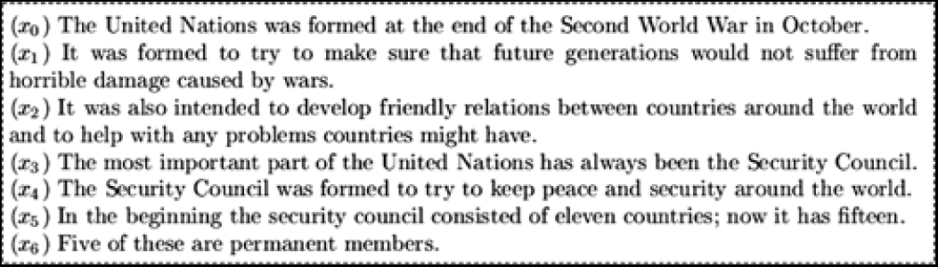
An example of a TD.

As an introductive example, let us consider the textual document depicted in Figure 1. For level l 1, we can obtain {members, damage, council, world, security} as textual features. For level l 2, they can be {nation-war, nation-world, council-nation, nation-security, council-world}. In this paper, we explain why and how these textual features are selected. It is organized as follows. In Section 2, we present the work related to TFS and their usefulness in TM applications. In Section 3, we provide the basic definitions related to FCA, RA, and TM. In Section 4, we present the links between N-composite isolated points and discovering information regularity for different levels. In Section 5, we introduce our new approach for TFS. In Section 6, we present the experimental results, and finally, in Section 7, we draw some conclusions and give some proposals for further work.
2. Related work
Several papers have already discussed the TFS literature review (Kosala and Blockeel Reference Kosala and Blockeel2000; Dasgupta et al. Reference Dasgupta, Drineas, Harb, Josifovski and Mahoney2007; Hasan and Ng Reference Hasan and Ng2014; Irfan et al. Reference Irfan, King, Grages, Ewen, Khan, Madani and Li2015). Basically, three main techniques for TFS have been widely used and categorized as follows: (i) BOW, (ii) BOP or bag of prototypical-phrases, and (iii) BOC. The BOW technique deals with all words in TDs (Witten et al. Reference Witten, Paynter, Frank, Gutwin and Nevill-Manning1999) without considering any correlation between them. In Yang and Pedersen (Reference Yang and Pedersen1997), a comparative study for five BOW selection methods concluded the strong correlation between document frequency, information gain, and χ2 statistics. As existing approaches, we could cite the single BOW and the single Keywords. In the single BOW, we use all words except for empty ones. The single Keywords are provided by experts in the field, as cited in Elloumi, Ferjani, and Jaoua (Reference Elloumi, Ferjani and Jaoua2016). Despite of their easy representation, the major limitations are (Salton and McGill Reference Salton and McGill1983):
BOW models not respecting the word semantics
Problem with collocations (juxtaposition of words)
Word combination and order generally ignored
Over-fitting and selecting a limited number of features
Our proposed approach extracts single BOW for 1-composite isolated points since we extract unique words. For BOP, the sequences of more occurring adjacent words are selected (Hasan and Ng Reference Hasan and Ng2014). These types of phrases, known as keyphrases, can be considered as highly relevant for describing a TD. A couple of examples of these approaches are KEA (Witten et al. Reference Witten, Paynter, Frank, Gutwin and Nevill-Manning1999) and Frequent-Term-Set (Agrawal, Imielinski, and Swami Reference Agrawal, Imielinski and Swami1993). The main characteristics of BOP are as follows:
They group all words that are interrelated.
Some are domain dependent, for instance, the approaches based on AGROVOC vocabulary (Rajbhandari and Keizer Reference Rajbhandari and Keizer2012).
In the Frequent-Term-Set approach, the frequent term set is extracted based on the Apriori algorithm (Agrawal, Imielinski, and Swami Reference Agrawal, Imielinski and Swami1993) where the parameters, support, and confidence are user predefined.
Redundant and infrequent terms could mislead the analysis and increase the complexity.
The last technique, BOC, focuses on the identification of surrounding words (i.e., word concept) for a given word present in a TD (Bernotas et al. Reference Bernotas, Karklius, Laurutis and Asta Slotkien2007). Some approaches have applied FCA on textual data and have extracted relevant textual features from FCs. They are considered BOC as well. In our approach, the set of N-composite isolated points constitutes one BOC. BOC are closely related to mathematical FCA settings. FCA has been shown to provide a theoretical framework for the efficient resolution of many practical problems from data mining (Rodriguez-Esteban Reference Rodriguez-Esteban2019), conceptual reasoning (Elloumi et al. Reference Elloumi, Boulifa, Jaoua, Saleh, Al Otaibi and Frias2014), software engineering, and information retrieval (Ganter and Wille Reference Ganter and Wille1999; Weiss et al. Reference Weiss2005; Jaoua et al. Reference Jaoua, AlJa’am, Hammami, Ferjani, Laban, Semmar, Essafi and Elloumi2010). An interesting problem is to find a representation of an FCT by minimal or an optimal set of concepts, particularly, in the case of textual data. Suppose that we have a set of documents (i.e., a corpus) that we need to explore and organize. The corpus could be represented by an FCT where the objects are documents and the properties are the words in the corpus, that is, BOW. An FC indicates a strong link between a subset of documents setdoc and a subset of words setw since they are completely interrelated. Each document d in setdoc has all words in setw. Conversely, each word w in setw should exists in all documents in setdoc. Finding a minimal representation of an FCT means the election of a minimal set Scov of concepts, called minimal coverage, where the union is the entire FCT xt, that is, the corpus. Finding the optimal coverage of a BR is known to be an NP-hard problem (Garey and Johnson Reference Garey and Johnson1979). Nevertheless, it could mean the election of optimal maximal rectangles (or equivalently FCs) that achieve maximal gain in storage space terms Jaoua et al. (Reference Jaoua, Elloumi, Hasnah, Jaam and Nafkha2004). Kcherif, Gammoudi, and Jaoua (Reference Kcherif, Gammoudi and Jaoua2000) introduced a rectangular decomposition approach based on the Riguet’s difunctional relation (Riguet 1948). The computation of this difunctional was reduced to the determination of a set of isolated points allowing the determination of the minimal set of rectangles covering a given BR. An extended isolated point-based version, called genCoverage, was proposed in Elloumi, Ferjani, and Jaoua (Reference Elloumi, Ferjani and Jaoua2016) by considering the extended context notion. Belohlavek and Vychodil (Reference Belohlavek and Vychodil2010) tackled the same issue by attempting to solve the Boolean factor analysis problem by proposing a new method of decomposing an n × m binary matrix I into a Boolean product A ○ B of an n × k binary matrix A and a k × m binary matrix B, where k is as small as possible. Mouakher and Ben Yahia (Reference Mouakher and Ben Yahia2016) introduced a new approach, based on a greedy algorithm, for the extraction of an optimal covering of a BR. The latter approach relied on the FC lattice representation. The guiding idea of Mouakher and Ben Yahia’s approach was that coverage should not be extracted regardless of the quality of knowledge that may be drawn from it. Therefore, the authors introduced a gain function based on the assessment of the correlation of the intent part of pertinent FCs. Generally, the number of FCs grows exponentially with the size of the matrix (i.e., BR)(Godin,Missaoui, and Alaoui Reference Godin, Missaoui and Alaoui1995). Fortunately, the use of mandatory concepts allows selecting an information with a minimal loss set of few relevant concepts in polynomial time. In this paper, we apply some existing conceptual approaches for BOC extraction. In particular, we cite:
Difunctional (Kcherif, Gammoudi, and Jaoua Reference Kcherif, Gammoudi and Jaoua2000): It is based on the exploration of the composed labels built on the Riguet difunctional relation (Riguet 1948).
Optimal factors (Belohlavek and Vychodil Reference Belohlavek and Vychodil2010): It explores the textual features as concept properties discovered by the optimal factor approach.
MinGenCoverage (Elloumi, Ferjani, and Jaoua Reference Elloumi, Ferjani and Jaoua2016): It considers the minimal generators as isolated-point candidates. Their corresponding isolated concepts are considered as composite labels.
3. Key settings
In the recent years, a large amount of research has concurrently explored the fields of computer science, RA, FCA, and lattice theory. These researches have enormously contributed to finding original solutions for complex problems in the fields of knowledge engineering, data mining, and information retrieval (Osei-Bryson Reference Osei-Bryson2010). Thus, RA and FCA are considered as useful mathematical foundations that have unified data and knowledge in information retrieval systems. In the following, we recall some basic definitions borrowed from RA as well as FCA.
3.1 FCA and textual data
FCA is a mathematical tool for analyzing data and formally representing conceptual knowledge. FCA helps to form conceptual structures from data. These structures, such as closed itemsets, generic bases, and minimal generators, are very useful for TM (Bastide et al. Reference Bastide, Pasquier, Taouil, Lakhal and Stumme2000). In the remainder of the paper, we use the theoretical framework presented in Ganter and Wille (Reference Ganter and Wille1999).
Definition 1. Formal Context: An FCT is a triplet  ${\cal K} = ({\cal X},{\cal Y},{\cal R})$, where
 ${\cal X}$ represents a finite set of objects or documents,
 ${\cal Y}$ is a finite set of attributes (or words), and
 ${\cal R}$ is a BR (i.e.,
 ${\cal R} \subseteq {\cal X} \times {\cal Y}$). Each pair
 $ \left( x,y \right) \in {\cal R}$ expresses that the document
 $x \in {\cal X}$ contains the word
 $y \in {\cal Y}$.
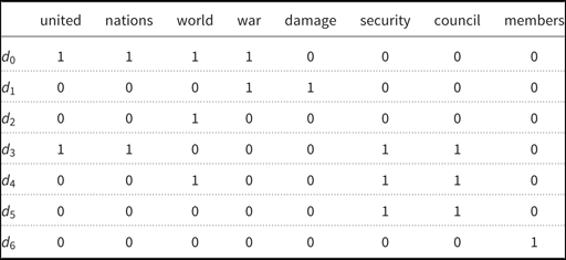
Example 1. Let  ${\cal X} = \{ {d_0},{d_1},{d_2},{d_3},{d_4},{d_5},{d_6}\}$ be a set of documents. Let ${\cal Y}$ = {united, nations, world, war, damage, security, council, members} be a set of words. In Table 1, we present an example of FCT relating the elements of ${\cal X}$ with those of ${\cal Y}$.
FCT representing the text presented in Table 1

Definition 2. Itemset: An itemset is a set of items, that is, words, included in ${\cal Y}$ and representing an object, that is, a document. An itemset is also called a termset. In the sequel, we denote by  ${\cal I}$ the power set of ${\cal Y}$.
Definition 3. Galois Connection: We define two functions f and g, summarizing the links between the subsets of documents and the subsets of words induced by ${\cal R}$. Thus,
 $f{\kern 1pt} :{\kern 1pt} {\cal P}({\cal X}) \to ({\cal P}({\cal Y}) = {\cal I}),\,f(X) = \{ y \in {\cal Y}|\forall x \in X,(x,y) \in {\cal R},X \subseteq {\cal X}\} $
- $g{\kern 1pt} :{\kern 1pt} ({\cal P}({\cal Y}) = {\cal I}) \to {\cal P}({\cal X}),\,g(Y) = \{ x \in {\cal X}|\forall y \in Y,(x,y) \in {\cal R},Y \subseteq {\cal Y}\} $.


Definition 4. Closed Itemset (Pasquier et al. Reference Pasquier, Bastide, Taouil and Lakhal1999): An itemset  $I\, \in \,{\cal I}$ is said to be closed if f ○ g(I) = I. f ○ g(I) is called a closure operator.
Definition 5. Formal Concept: An FC C = (A, B) is a pair where  $A \subseteq {\cal X},B \subseteq {\cal Y}$, A = g(B), and B = f (A) Set A is called the extent of C and set B is called its intent (Ganter and Wille Reference Ganter and Wille1999). An FC is also called a maximal rectangle or a non-enlargeable rectangle (Jaoua et al. Reference Jaoua, Elloumi, Hasnah, Jaam and Nafkha2004).
Example 2. From the FCT presented in Table 1, the following pair C 1 = (A, B) = ({d 3, d 4, d 5}, {security, council}) is an FC since f(A) = B and g(B) = A. Set B is a closed itemset. Note that all documents in A have all the words in B. Conversely, all words in B belong to all documents in A.
Remark 1. From any FCT, it is possible to locate several FCs covering it, that is, the union of FCs is equal to FCT.
Example 3. By considering the Table 1, we obtain the coverage Coverage 1 = {C 0, C 1, C 2, C 3, C 4, C 5, C 6} where :
C 0 = ({d 0}, {nation, united, war, world})
C 1 = ({d 0, d 2, d 4}, {world})
C 2 = ({d 1}, {damage, war})
C 3 = ({d 3}, {council, nation, security, united})
C 4 = ({d 3, d 4, d 5}, {security, council})
C 5 = ({d 4}, {council, security, world})
C 6 = ({d 6}, {members})
Example 4. From Table 1, we obtain  $Coverag{e_2} = \{ {C'_0},{C'_1},{C'_2},{C'_3},{C'_4},{C'_5}\} $
- ${C'_0} = (\{ {d_0},{d_3}\} ,\{ nation,united\} )$
- ${C'_1} = (\{ {d_0},{d_2},{d_4}\} ,\{ world\} )$
- ${C'_2} = (\{ {d_0},{d_1}\} ,\{ war\} )$
- ${C'_3} = (\{ {d_1}\} ,\{ war,damage\} )$
- ${C'_4} = (\{ {d_3},{d_4},{d_5}\} ,\{ security,council\} )$
- ${C'_5} = (\{ {d_6}\} ,\{ members\} )$


Remark 2. In (Mouakher and Ben Yahia Reference Mouakher and Ben Yahia2016) the authors discussed the coverage quality by considering different metrics applied to their FCs, such as coupling, cohesion, gain, stability, etc. From Examples 3 and 4, two types of distinct coverage were obtained. In general, varied coverage could be obtained while processing any FCT. Furthermore, in Belohlavek and Vychodil (Reference Belohlavek and Vychodil2010), it was mentioned that certain FCs were mandatory in that they needed to be included in every coverage stage. For instance, the FCs  ${C_1} = {C'_1}$,
 ${C_4} = {C'_4}$ and
 ${C_6} = {C'_5}$ are mandatory. In this paper, we defend the idea that the labels of these mandatory FCs constitute the first set of textual features. In the following, we introduce the mathematical basis related to difunctionality for locating these concepts based on property composition.
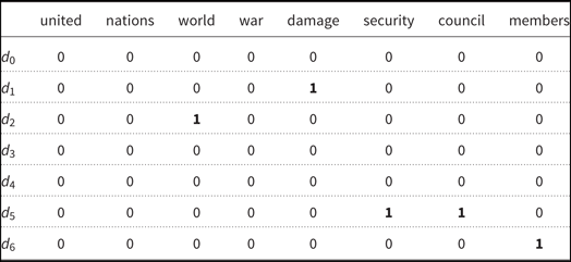
Fringe relation corresponding to BR presented in Table

3.2 Difunctionality
In the sequel, we recall some important definitions related to difunctionality, as a closed notion to an uniformity aspect, which we may find or extract from BRs. We focus on difunctional and fringe relations. Let us consider two sets, ${\cal X}$ and ${\cal Y}$, a relation ${\cal R}$, as a subset of the Cartesian product of ${\cal X}$ and ${\cal Y}$, and two elements e, e′ where  $e \in {\cal X}$ and
 $e' \in {\cal Y}$. We start by presenting these basic definitions (Ganter and Wille Reference Ganter and Wille1999):
The relative product or composition of two BRs
${\cal R}$ and ${\cal R}'$ is ${\cal R} \circ {\cal R}' = \{ (e,e')|\exists t \in {\cal Y}{\kern 1pt} :{\kern 1pt} ((e,t) \in {\cal R}) \, and \, ((t,e') \in {\cal R}')\} $.The inverse of relation
${\cal R}$ is ${{\cal R}^{ - 1}} = \{ (e,e')|(e',e) \in {\cal R}\} $.The complement of relation
${\cal R}$ is $\overline {\cal R} = \{ (e,e')|(e,e') \notin {\cal R}\} $.


Definition 6. Difunctional Relation (Ganter and Wille Reference Ganter and Wille1999): Let ${\cal R}$ be a BR. ${\cal R}$ is said to be difunctional if  ${\cal R} \circ {{\cal R}^{ - 1}} \circ {\cal R} = {\cal R}$. ${\cal R}$ can be written in a block diagonal form by suitably rearranging rows and columns. This means that a difunctional relation presents the uniformity of the association of images and antecedents.
Even though a BR is not always uniform as difunctional, Riguet has proved that there is an interesting difunctional embedded in it, which is generally not empty (Riguet 1948). This relation is called a fringe relation that we define in the following.
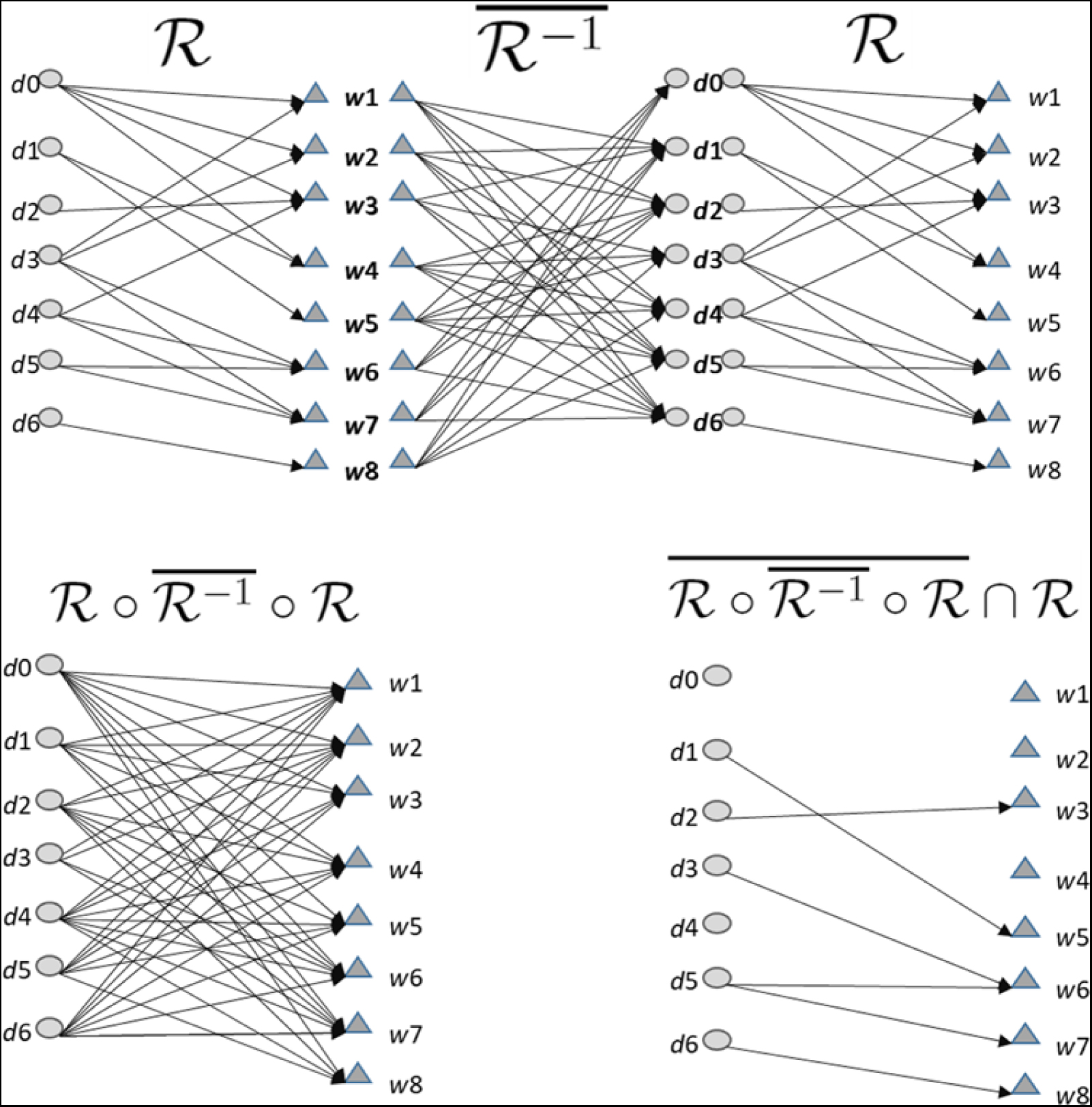
Steps for obtaining the fringe relation corresponding to the BR presented in Table 1.

Definition 7. Fringe Relation (Riguet 1948): A fringe relation is a difunctional relation embedded in a BR ${\cal R}$ and computed by  $\overline {{\cal R} \circ \overline {{{\cal R}^{ - 1}}} \circ {\cal R}} \cap {\cal R}$. It is denoted as
 ${{\cal R}_d}$. Moreover, a fringe relation is composed by a set of points contained in just one maximal rectangle inside relation ${\cal R}$ which can play an important role in different applications.
Example 5. In Table 2, we present the fringe relation corresponding to the ${\cal R}$ BR illustrated in Table 1. The difunctionality aspect is observed in the fringe relation as a sparse subrelation.
Remark 3. To understand the formula $\overline {{\cal R} \circ \overline {{{\cal R}^{ - 1}}} \circ {\cal R}} \cap {\cal R}$, we present in Figure 2 the steps for obtaining the fringe relation corresponding to the BR presented in Table 1. The words wt, t = 1 … 8, correspond the BR words. For example, w 1=united, w 2= nations.
Relation
${\cal R}$ is relating documents to their words. For instance, d 5 has two words: w 6 and w 7. Hence, the pairs (d 5, w 6) and (d 5, w 7) belong to ${\cal R}$.Relation
$\overline {{{\cal R}^{ - 1}}} $ relates documents to words which are not related in ${\cal R}$. For instance, it contains the pairs (d 5, w 1), (d 5, w 2), (d 5, w 3), (d 5, w 4), (d 5, w 5), (d 5, w 8).Relation
${\cal R} \circ \overline {{{\cal R}^{ - 1}}} $ produces a relation between documents di and dj if there exists at least one word in di and not in dj. For instance, we get pairs (d 5, d 0), (s 5, d 1), (d 5, d 2) (d 5, d 3), (d 5, d 4), (d 5, d 6)Relation
${\cal R} \circ \overline {{{\cal R}^{ - 1}}} \circ {\cal R}$ relates documents to words, say (di, wt), for wt not in di if there exists at least a document dj having wt while having other words not existing in di. For example, we get the pairs (d 5, w 1), (d 5, w 2), (d 5, w 3), (d 5, w 4), (d 5, w 5), (d 5, w 8).Relation
$\overline {{\cal R} \circ \overline {{{\cal R}^{ - 1}}} \circ {\cal R}} \cap {\cal R}$ expresses the negation of the previous condition. It means that if di is connected to wt, then for all documents having wt di will have no connection with any of the other words, for example, we get the pair (d 5, w 6) and (d 5, w 7).


The elements belonging to a fringe relation are called isolated points and their usefulness are shown in extracting concept’s labels and TFS (Elloumi, Ferjani, and Jaoua Reference Elloumi, Ferjani and Jaoua2016).
4. Isolated points and N-composite isolated points
In this section, we present the necessary definitions related to isolated points. We recall some of their useful properties and we present novel issues for obtaining N-composite ones as relevant textual features.
Definition 8. Isolated Point Kcherif et al. (Reference Kcherif, Gammoudi and Jaoua2000): Let ${\cal R}$ be a BR and ${{\cal R}_d}$ be its associated fringe relation. If  $p = (x,y) \in {{\cal R}_d}$, then p is called an isolated point. An isolated point belongs to only one FC and the latter is called an isolated concept.
Example 6. With respect to the BR presented in Table 1, the FC C = (A, B) = ({d 3, d 4, d 5,}, {security, council}) is an isolated one since (d 5, council) is an isolated point.
Proposition 1. (Ferjani et al. Reference Ferjani, Elloumi, Jaoua, Ben Yahia, Ismail and Ravan2012). Let p = (x, y) be an isolated point in an FC C = (A, B). The following properties are satisfied:

Remark 4. From proposition 1, particularly, the expression f ○ g({y}) = B means that if a document d in ${\cal X}$ contains the word y, then it contains necessarily all words in B. Thus, we have the implication y → B\ {y}. The word y can be selected as an interesting candidate representing all words in B since they are implied by y.
Definition 9. Concept Label: If  $p = (x,y) \in {\cal R}$ is an isolated point in an isolated concept C, then y is called a concept label of C.
Example 7. The word council is selected as a concept label of C 4, and the implication council → security is true.
Remark 5. For textual data, the labels can reflect the indexing words or text features (Ferjani et al. Reference Ferjani, Elloumi, Jaoua, Ben Yahia, Ismail and Ravan2012). In many cases, no single label can be associated with an FC since it does not contain single isolated points. To overcome this situation, we suggest composite properties as candidates for concept labeling. In this paper, we propose to consider N-composite properties to discover the composite labels. We formalize these ideas in the following.
Definition 10. Composite Properties (Ferjani et al. Reference Ferjani, Elloumi, Jaoua, Ben Yahia, Ismail and Ravan2012): Let  $({\cal X},{\cal Y},{\cal R})$ be an FCT, and let
 $SP \subseteq {\cal Y}$, that is, a subset of properties such that |SP| ≥ 2. A composition of the properties of SP defines a new composite property, denoted by CPSP = p 1.p 2…pn, n = |SP|, pi ∈ SP, i = 1…n, which can be added to set ${\cal Y}$. This new property CPSP can be used to define an extended context as well as to select a composite label for an FC when a single label cannot be assigned.
Definition 11. N -Composite Property: Let N be a positive integer and $SP \subseteq {\cal Y}$. An N-composite property denoted by NCPSP is a CPSP such that |SP| = N.
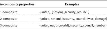
Example 8. Let us consider the FCT presented in Table 1. In Table 3, we present examples of 1-composite, 2-composite, and 3-composite properties or words.
Composite words extracted for different levels

Definition 12. Expanded Context: Let  $FC = ({\cal X},{\cal Y},{\cal R})$ be an FCT and let NCPSP be an N-composite property. NCPSP can be added to set ${\cal Y}$ to define an expanded context:
 $EX{P_{(FC,SP)}} = ({\cal X},{\cal Y} \cup NC{P_{SP}},{\cal R}')$ where R′ = R ∪ {(x, NCPSP)|(x, y) ∈ R, ∀y ∈ SP}.
Definition 13. N -Composite Property Isolated Point: Let $FC = ({\cal X},{\cal Y},{\cal R})$ and NCPSP be an N-composite property. NCPSP is an N-composite isolated point if there exists  $x \in {\cal X}|(x,NC{P_{SP}})$ which is an isolated point in the expanded context EXP (FC, SP ).
Remark 6. Why is it important to compose properties?
There are two main reasons:
Discover the hidden regularity in the data implied by the N-composite isolated points. Therefore, it would be selected as a textual feature.
Discover additional isolated concepts in order to cover more documents in a corpus. Note that for TFS, the coverage criteria is not the most important aspect. We are more focusing on extracting representative textual features without having necessarily 100% of coverage percentage.
Remark 7. How can we compose properties?
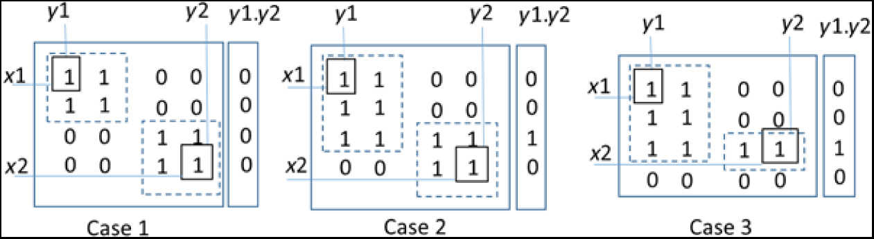
Three cases for isolated-point compositions.

The isolated points have some important properties that will prevent any randomized word combination. In particular, we will check whether some word combinations are useless or not, mainly when isolated points are involved. Let us consider Figure 3 in which we distinguish three cases for isolated-point combination. In each case, we have two isolated points (x 1, y1), (x 2, y2) and their corresponding FC marked by dotted rectangles. y 1. y 2 denotes the 2-composite property obtained from {y 1, y 2}. We have:
Case 1: The isolated points belong to two distinct concepts. Therefore, the intersection between g({y 1}) and g({y 2}) is empty, and it is useless to make the isolated-point composition. Proposition 2 formalizes case 1.
Case 2: The intersection between g({y 1}) and g({y 2}) is not empty and we will check if some additional isolated points might be derived when considering y 1. y 2.
Case 3: Even if the intersection of g({y 1}) and g({y 2}) is not empty, their composition is useless. In fact, the isolated point (x 2, y 2) belongs to an already covered concept. Here, the proof is trivial since an isolated point belongs to a unique concept.
Proposition 2. Let p 1 = (x 1, y 1) and p 2 = (x 2, y 2) be two isolated points in two distinct concepts C 1 = (A 1, B 1) and C 2 = (A 2, B 2). Let SP = {y 1, y 2} and 2CPSP its corresponding 2-composite property. The following property is satisfied:
If A 1 ∩ A 2 = ∅, then 2CPSP is empty; that is, g({SP}) = ∅. In other words, no 2-composite isolated point is derivable.
Proof.  ${g}(SP) = \{ x \in {\cal X}|\forall y \in \{ {y_1},{y_2}\} ,(x,y) \in {\cal R},Y \subseteq {\cal Y}\} $
=  $ = \{ x \in {\cal X}|(x,{y_1}) \in {\cal R} \wedge (x,{y_2}) \in {\cal R}\} $
= g(y1) ∩ g(y 2) by definition
= A 1 ∩ A 2 = ∅ by hypothesis. □
Remark 8. This property is important in the property composition algorithm. It shows that it is useless to make a composition between two isolated points when they belong to two distinct concepts. Moreover, the composition would give isolated points where all related concept’s elements were covered.
Remark 9. As long as we increase the value of N, for the N-composite properties, the possibly isolated N-composite points and their associated FCs are covering additional elements in the BR. Generally, for TFS, when the size of data is big, it is recommended to limit the value of N to a small value (e.g., 2 or 3) even for non-covering the whole relation. Hence, combining non-isolated properties will give newly isolated points.
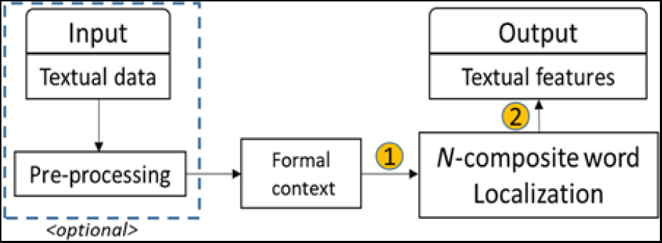
Features extraction process.

5. Using N-composite isolated points for textual feature selection
This section represents our contribution in this paper. We start by presenting the system architecture, as depicted in Figure 4, and we develop the N-composite word localization algorithm for TFS.
5.1 System architecture
We propose to extract the textual features by the steps (1) and (2) as illustrated in Figure 4. From the processed textual data, we obtain an FCT relating documents to words. For a level i from 1 to N, we iteratively locate the isolated i-composite words as indicated in Algorithm 1. Their union is the set of textual features.
In the case of new collected data sets, for example, the data collected in the scope of the Financial Watch Project (FW-Data)(Jaoua et al. Reference Jaoua, AlJa’am, Hammami, Ferjani, Laban, Semmar, Essafi and Elloumi2010), we recommend to apply a pre-processing phase before starting the TFS as indicated in the < optional > step. It consists in applying the natural language processing steps (e.g., stopword removal, synonymy processing) to prepare the FCT construction. This step is important before transforming the textual data into an FCT. In several benchmark data sets, this step has been already done for some versions. For instance, it is the case of the 20-newsgroup data sets (Rennie Reference Rennie2008) which are easy to read into Matlab/Octave as a sparse matrix. Hence, we just need to rearrange data into our algorithm input format.
5.2 Main algorithm
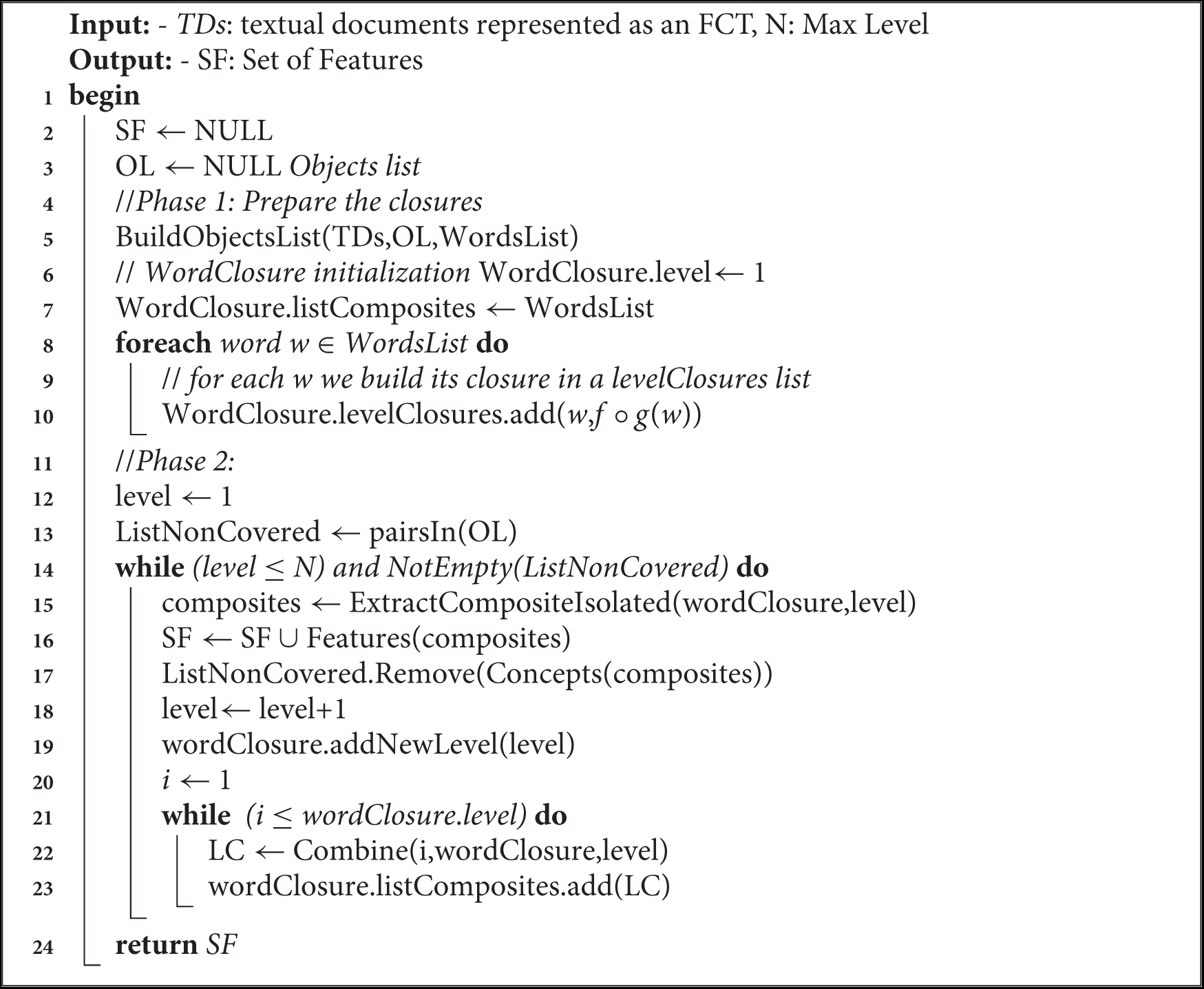
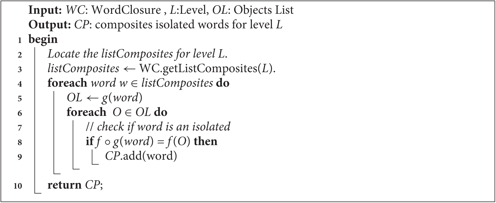
The pseudo-code presented in Algorithm 1 reflects the steps we follow to compute the N-composite isolated properties and to extract the textual features. First, we identify the set of isolated points and their corresponding concepts. If the FCT is not covered and the composition level N is not reached, then we iterate on the remaining set of composite words and keep only those representing the isolated points.
In lines 2–10, we prepare the closure sets related to documents and words, respectively. The routine BuildObjectsList constructs OL and WordsList as follows:
– OL: It has an hMap structure or a dictionary (as defined in Python), where, OL ← {obj: f(obj) for obj inTDs}. f(obj) is the list of words in obj.
– WordsList is the set of all words in TDs.
For each word w in WordsList, we compute g(w) and its closure f ○ g(w). This result is added to the levelClosures list defined within WordClosure. As long as the level increases, we get level-composite words. Hence, the variable WordClosure stores the composition level and the closures of the level-composite words in levelClosures.
In lines 12–18, we locate the current level-composite isolated point w.r.t. the properties presented in Proposition 1. We update the set of features SF and we remove the covered elements from the set ListNonCovered. The ExtractCompositeIsolated routine considers Proposition 1 and makes a traversal of Wordclosure.levelClosures in order to identify the isolated composite points. Note that for level 1, composites represent the 1-composite isolated points. The Feature routine extracts the words of isolated points. The routine Concepts returns a set of pairs setP = {(object, word)} forming the FC associated with composites. The elements of setP are removed from ListNonCovered to check the coverage condition.
In lines 19–23, the routine combine combines (the new level value) words as new candidates of isolated composite points based on the previous level-composite elements. For instance, suppose for level 2, we have the composite properties {w 1.w 2, w 2.w 3, w 3.w 4}, then, for level 3, we get {w 1.w 2.w 3, w 1.w 2.w 4, w 2.w 3.w 4}. In order to reduce the combinatory number, we consider Remark 7 and Proposition 2.
5.2.1 Complexity analysis
Let  $n = |{\cal X}|$ and
 $m = |{\cal Y}|$ be, respectively, the number of documents and the number of words in the TDs.
In phase 1, the procedures BuildObjectsList and the construction of WordClosure require n × m operations.
In phase 2, the algorithm performs the WordClosure.levelClosures traversal and locates the level-composite isolated points by applying the ExtractCompositesIsolated function. In the worst case, we have M = max(N, MaxLevel) where N is the number of traversals and MaxLevel is the max level specified by a user. Let us consider a composition level i for which |WordClosure.levelClosures| =mi. The WordClosure.levelClosures property composition requires
${m_i} + ({m_i} - 1) + ({m_i} - 2) + \cdots + 1 = {{{m_i}({m_i} + 1)} \over 2}$ operations. Hence, there are $\sum\limits_{i = 1}^M {{{m_i}({m_i} + 1)} \over 2}$ operations.


TFS algorithm

5.2.2 Illustrative example
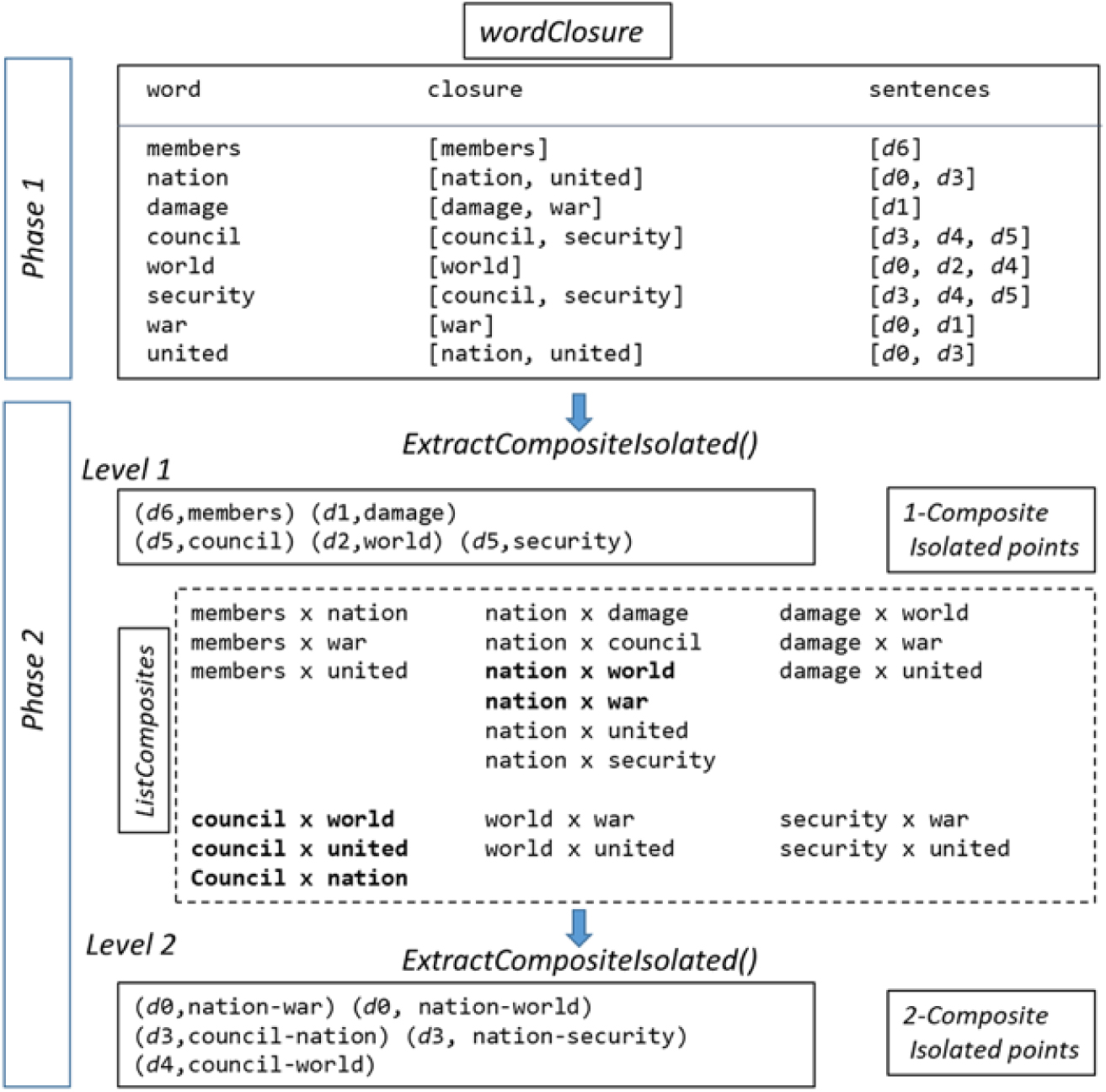
Let us reconsider the FCT given by Table 1. Figure 5 illustrates the different phases of Algorithm 1. In phase 1, the wordClosure list is constructed. It contains the words, their closures, and their associated documents obtained by the Galois connection. In phase 2, we have two levels. At level 1, the ExtractCompositeIsolated routine returns the set of isolated 1-composite points. At level 2, the combine routine combines two words w.r.t. Remark 7 and Proposition 2 and returns ListComposites. The latter represents the new candidates of isolated composite points. In the second iteration, the ExtractCompositeIsolated returns the isolated 2-composite points and the FCT is entirely covered.
ExtractCompositesIsolated function

Illustrative example.

5.2.3 Discussion
The TFS algorithm output represents the set of isolated concepts with their labels. Hence, we have two results: (i) It is partial-total FCT coverage, so it informs about the coverage percentage. (ii) It represents single and possibly composite textual features reducing the TDs dimensionality. Consequently, we need to be informed about their relevance by using appropriate metrics.
(i) Partial-total FCT coverage: As we can see in Example 5, at level 1, the isolated 1-composite points are associated with the concepts {C 1, C 2, C 4, C 6} as listed in Example 3. They cover 12/17 or (70.58%) elements in the FCT given by Table 1. At level 2, the isolated 2-composite points are associated with the additional concepts {C 0, C 3, C 5}. As a result, we get 100% coverage.
(ii) Single and composite properties: With respect to Example 5, at level 1, we get five 1-composite isolated points, that is, five selected features. Thus, we have 3/8 or 37.50% as a reduction rate. The words council and security belong to the same concept C 4 so, we can consider the option to keep only one of them and reach a 50.00% reduction rate while covering (70.58%) elements in the FCT. At level 2, the coverage percentage is 100%. Even if the number of isolated 2-composite points is 5, some of them are equivalent as they belong to the same concept. For instance, it is the case of (d 0, nation-war) and (d 0, nation-world). In total, we have at least three additional features.
Remark 10. In this paper, we process all selected features without considering the equivalence between some of them.
6. Experiments
We start by introducing the used textual data sets and the evaluations metrics we used for evaluating the extracted-textual-feature relevance for different composition levels. After that, we present the experimental results.
6.1 Textual data sets
We have considered two data sets: the FW-Data (Jaoua et al. Reference Jaoua, AlJa’am, Hammami, Ferjani, Laban, Semmar, Essafi and Elloumi2010) and the 20-newsgroup data sets (Rennie Reference Rennie2008) (Matlab/Octave version).
FW-Data
FW-Data is a collection of approximately 400 TDs collected in the scope of the Financial Watch Project (Jaoua et al. Reference Jaoua, AlJa’am, Hammami, Ferjani, Laban, Semmar, Essafi and Elloumi2010) with the collaboration of the CEA-LIST institute.Footnote a The documents have been already classified in three categories according to the predefined classes in the financial domain which are management change, performance, and transaction. The collected data have been analyzed and annotated by experts in order to build a multilingual platform for knowledge discovery, information extraction, and automatic translation in the financial domain. The pre-processing step is performed as it is new collected data. More particularly, we apply the Standford POS tagger tool (Manning et al. Reference Manning, Surdeanu, Bauer, Finkel, Bethard and McClosky2014) for annotating text with part-of-speech information. Furthermore, we apply a transformation process for getting a uniform representation for some phrases. For example, the phrases “Qatar National Bank,” “National Bank,” and “QNB” designate the same bank and should be represented by a unique way. Also, we apply the Porter Stemmer algorithm to reduce a token to its root form (Porter Reference Porter1980). For synonym processing, we create a synonym table and feed it with processed noun entries, captured from Wordnet3 (Miller Reference Miller1995). Our synonym table contains around 427,000 entries. It is composed of three attributes: IdWord, word, and IdR, where:
IdWord is the word identifier. It is incrementally obtained while processing the entries.
word is the stem of the processed word entry.
IdR is the identifier of its representative word.
In the synonym table, each word has a unique representative one. Thus, the synonym table construction algorithm considers three cases:
Case 1: Add non existing sets of synonyms to the table of synonyms.
Case 2: Enlarge the set of synonyms having the same representative word. Hence, we will get new rows in the table.
Case 3: Ignore the conflictual cases. These cases correspond to a new entry from Wordnet3 having at least two words already saved in the synonym table and having two distinct representative words.
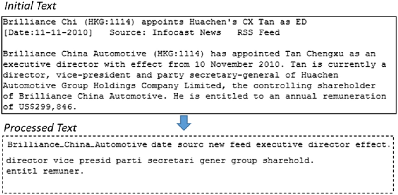
As an illustration, we present in Figure 6 an example of a processed text for the management change class.
Characteristics of FW-Data

Statistical significance of the differences between FW-Data groups

Example of management change text and its transformation.

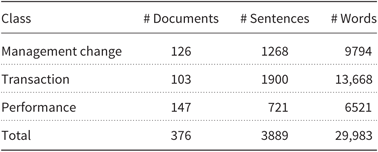
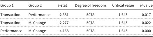
There exist also other techniques for finding the similarity between words by considering embedding models such as the GloVe approach (Pennington, Socher, and Manning Reference Pennington, Socher and Manning2014) and the one estimating the word representation (Mikolov et al. Reference Mikolov, Chen, Corrado and Dean2013). In Table 4, we present the main characteristics of the FW-Data. For each class, we indicate the number of documents, the number of sentences, and the number of words. In addition, we present in Table 5 the statistical significance of the differences between the three groups in FW-Data. The t-test, or student’s t-test (Gosset Reference Gosset1908), is an inferential statistical test that determines whether there is a statistically significant difference between the means in two unrelated groups. The significance level (also called alpha) is set to 0.05. It allows to decide to either reject or accept the null hypothesis, that is, that the population means from the two unrelated groups are equal. Form Table 5, we remark that, in all cases, the absolute value of t-stat is greater than the critical value. Also, we have P is less than alpha. These observations converge to conclude to reject the null hypothesis that the means are equal.
20-newsgroups data set
We have considered the (Matlab/Octave) version which has been already a processed data set. It contains both training and testing sets. We convert the training file to our TFS-algorithm input without considering the class attribute. It is a BR composed of 53,975 words and 11,269 objects.
6.2 Evaluation metrics
We propose to evaluate the extracted-textual-feature relevance by considering the standard measures used for supervised classification. For textual data, the classes are the documents categories. Hence, the metrics are Precision, Recall, F-measure, micro-average accuracy, and macro-average accuracy (Gordon and Kochen Reference Gordon and Kochen1998). Let us consider N the number of categories in a textual data set and i ∈ N a given category. The metrics use the parameters TPi, FPi, and FNi standing for true positive, false positive, and false negative for a class i, respectively. They are computed as following:
- ${\rm{Precisio}}{{\rm{n}}_i} = {{T{P_i}} \over {T{P_i} + F{P_i}}}$
- ${\rm{Recal}}{{\rm{l}}_i} = {{T{P_i}} \over {T{P_i} + F{N_i}}}$
- $F\_{\rm{measur}}{{\rm{e}}_i} = {{2 \times {\rm{P}}recisio{n_i} \times {\rm{R}}ecal{l_i}} \over {{\rm{P}}recisio{n_i} + {\rm{R}}ecal{l_i}}}$
- ${\rm{Micro}} - {\rm{average \, accuracy}} = \sum\nolimits_{i = 1}^N {{T{P_i}} \over {T{P_i} + F{P_i}}}$
- ${\rm{Macro}} - {\rm{average \, accuracy}} = \sum\nolimits_{i = 1}^N {{{\rm{P}}recisio{n_i}} \over N}$


6.3 Evaluation of extracted-textual-feature relevance
The evaluation of the extracted-textual-feature relevance is based on their number w.r.t. composition levels and on the evaluation metrics as presented in Section 6.2. To evaluate our approaches compared to others, LIBSVM is used (Chang and Lin Reference Chang and Lin2011) as an integrated approach to the Rapidminer software tool (KDnuggets 2012) installed on a personal computer with a 2.3 GHz CPU, 8 GB of RAM, and Windows 7.
6.3.1 Results for FW-Data
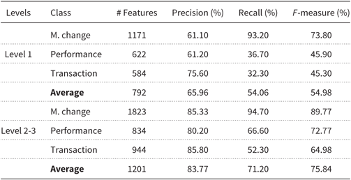
We start by presenting the level impact for the coverage percentage for FW-Data. For each level, we obtain a set of features whose efficiency is to be experimented. Furthermore, we present the evaluation of the approach of isolated N-composite points compared to other ones, as cited in the related work. In Table 6, we present the evaluation of the approach of isolated N-composite points for different levels and classes applied on the FW-Data. As we could remark, the composite properties have a positive impact on the precision–recall values for all classes. Hence, combining two words is very significant to reach acceptable classification accuracy. Regarding the total number of extracted features for all classes, we have (790) 1-composite and (1570) 2-composites covering 46.82% and 98.50% of FCT, respectively. Obviously, these values do not correspond necessarily to the summation of different features in the different classes, since the redundancies are eliminated. For level 3, only six additional features were obtained. Hence, for all classes, their total number is 2366. The management change class has the best values compared with the other classes, whereas the transaction class has the lowest values. The micro-average precisions are 67.08% and 83.05% for level 1 and levels 2 and 3, respectively. The macro-average precision for level 1 is 65.96% and 83.77% for levels 2 and 3.
Evaluation for different levels w.r.t. FW-Data classes

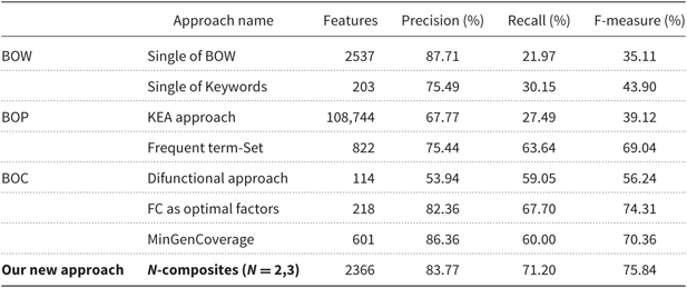
In Table 7, we present the results of the evaluation of the approach of isolated N-composite points compared to the other ones as cited in Ferjani et al. (Reference Ferjani, Elloumi, Jaoua, Ben Yahia, Ismail and Ravan2012) and Elloumi et al. (Reference Elloumi, Ferjani and Jaoua2016) based on the precision/recall metrics. In this paper, we are particularly interested in comparing between conceptual approaches as we put forward a new version for extracting the isolated concepts.
Results of different approaches for FW-Data

In this study, we use Rapidminer (KDnuggets 2012) and the linear support vector machine (SVM) (Chang and Lin Reference Chang and Lin2011) as a classifier with 10-folds in order to evaluate the different approaches. We calculate the precision, recall, and F-measure for the different approaches, as depicted in Table 7. It can be clearly seen that the precision varies from 53.94% to 87.71% (with a gap approximately equal to 33.77%) and the recall varies from 21.97% to 71.26% (with a gap around 49.29%) where the highest recall value is observed for the proposed new approach for N=2,3. The most striking feature is that (single of keywords) the keywords have been manually extracted by experts which does not give the highest precision 87.71%. In addition, the recall is very low (30.15%). This could be explained by the limited number of features suggested by the expert (218 labels are extracted) which are not as representatives as expected. Note that the recall, which describes what proportion of TDs that should be classified as yes and in fact classified as yes is very low in the BOW (21.97%). Regarding the conceptual approaches, the MinGenCoverage presents the best precision value (86.33%). In the new proposed approach, both precision/recall measurements are greater than 70.00%. Hence, the selected features composed of 790 single words and 1576 2–3-composite words are significant features w.r.t. the whole textual data.
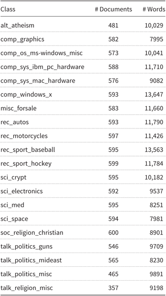
Characteristics of 20-newsgroup data set

Evaluation for different levels w.r.t. 20-newsgroup classes

6.3.2 Results for 20-newsgroup
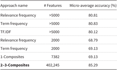
We consider the (Matlab/Octave) version which is already a processed data set. It contains both training and testing sets. We have converted the training file to our TFS-algorithm input without considering the class attribute. It is a BR composed of 53,975 words and 11,269 objects. As results, we have 7382 1-isolated points covering 100% of the BR. This informs about the sparseness of the 20-newsgroup data set since the BR is completely covered at level 1. In Table 8, we present some characteristics of the 20-news data sets in terms of number of documents and number of words per document. We apply the nltk.PlaintextCorpusReader (Bird and Loper Reference Bird and Loper2004) to extract the BOW for each class. Note that the requested time in average to extract the composite features is around 3 min per class. We remark that the number of 1-composites represents 4.69% of the entire number of words which could be interesting for the dimensionality reduction problem. However, the number of 2-composites goes up by more than 112%, which constitutes a drawback from the dimensionality reduction perspective. Nevertheless, it could be useful for constituting BOP where words are grouped w.r.t. the isolated composite aspect as a means of discovering more regularities in a corpus. Regarding the total number of extracted features for all classes we have 7382 distinct features for level 1 and 402,245 distinct ones for level 2.
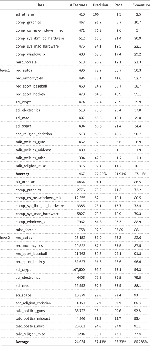
As illustrated in Table 9, we can remark that the precision levels range from 42.9% to 100% where 9/20 classes have more than 84%. However, the recall values are low except for the basketball class. In average, the macro-average precision for level 1 is 77.20% and the micro-average precision is 66.35%. These results indicate that the isolated 1-composite points produce acceptable precision levels but they are not discriminating the classes. For level 2, we got 87.43% for macro-average precision and 85.29% for micro-average precision.
In Table 10, we present the obtained results for different approaches, as cited in Lan, Tan, and Low (Reference Lan, Tan and Low2006) in terms of micro-average accuracy. For relevance frequency and term frequency, we present two results related to the considered number of features (i.e., > 5000 and 2000). This result indicates the positive impact of using a greater number of features as an increase accuracy from 69.13% up to 80.83%. The two last rows in Table 10 concern the results obtained by our new approach for levels 1 and 2. The number of features at level 2 is approximately 50 times that of level 1. This could be disadvantageous in terms of dimensionality aspect, but accuracy rises from 69.13% up to 85.29%. When we analyze the training set, we observe that many objects have a zero value for all features. Accordingly, the isolated 1-composite points do not exist for these objects. Moreover, some features are present in different objects even if they are not within the same class. These features are misleading and an additional filtering step could be considered to remove them. By considering the isolated 2-composite points, the accuracy is improved which witnesses the usefulness of considering the additional features during the learning stage. We are confident that it is worth studying many alternatives in property composition algorithm in order to extract more relevant features.
Results of different approaches for 20-newsgroup data set

7. Conclusion
Textual data processing requires well-found approaches to derive relevant textual features. In this paper, we have put forward a new approach for TFS based on FCA background. Mainly, we have proposed to extract textual features by exploring the Riguet-difunctional relation. It allows discovering the regularities in an FCT as a set of isolated points. These regularities are also expressed as logical implications between words within the same concept. As a main contribution, we have introduced the notion of isolated N-composite points as a set of N words to be considered as a unique textual feature. In addition, we have suggested some key elements for avoiding the composition of useless words in the TFS algorithm. From the experimental results, we have concluded that a reduced value of N (between 1 and 3) permits extracting significant textual features compared with existing approaches even for not completely covering the initial FCT. Nevertheless, we need to explore the relation between the coverage quality and the relevance of textual features. As for further work, we are confident that the proposed approach can contribute to analyzing large textual corpora more efficiently and to be extended for a multi-language aspect.
Author ORCID
S. Elloumi, 0000-0002-1822-5334