1 Introduction
Looking into nature one can find some outstanding inventions that have been a result of millions of years of evolution. Engineers often look there to find inspiration for modern technological solutions. In this paper a work that is inspired by the flippers of the humpback whale will be presented. These large mammals are known to have excellent hydrodynamic capabilities, in particular for manoeuvring. They are fast and agile and that can be partially attributed to a specific shape of their flippers. While for most of the sea mammals flippers are shaped as smooth hydrofoils, the flipper’s leading edge in the humpback whale has a series of ‘bumps’ called tubercles. Ongoing research has been focused on understanding the action of these tubercled foils to see if they can be successfully implemented in engineering design.
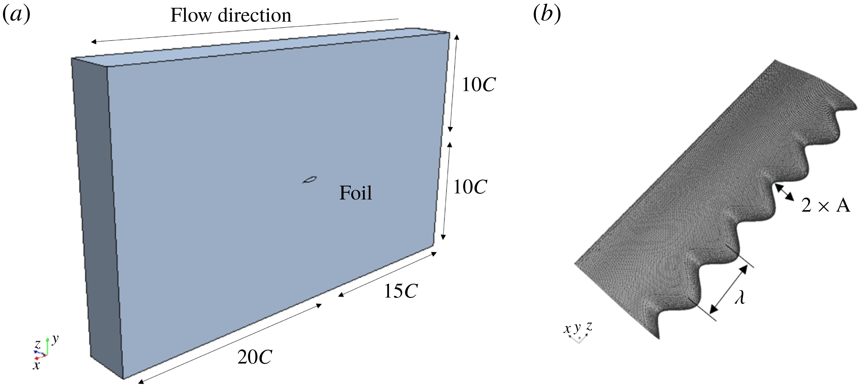
Such tubercles were first researched and described as natural lift enhancement devices by Fish & Battle (Reference Fish and Battle1995) who recognised that the presence of tubercles on a flipper can delay the stall, allowing the flipper to maintain a high lift coefficient at high angles of attack. Other researchers looked at the impact of the shape on the performance of the humpback whale flipper. For example, Miklosovic et al. (Reference Miklosovic, Murray, Howle and Fish2004) experimentally tested three flipper shapes with and without tubercles. They found that, by the introduction of tubercles, an increase in the maximum produced lift and in the stall angle was achieved. It was also found that at certain angles of attack the drag decreased as well. In addition, Miklosovic, Murray & Howle (Reference Miklosovic, Murray and Howle2007), concluded that tubercle behaviour is dependent on wing overall shape as well. Likewise, Johari et al. (Reference Johari, Henoch, Custodio and Levshin2007) conducted the experimental evaluation of NACA shaped section wings with a smooth leading edge (without tubercles) and with leading edge tubercles having a range of the tubercle wave amplitude (see figure 1 b). They highlighted that the best hydrodynamic performance was achieved by the foil with the smallest wave amplitude.
Although previous research showed a strong dependence on tubercle geometry and foil shape, as expected the main factor affecting the performance of tubercled foils is the Reynolds number (
 $Re$
). Stanway (Reference Stanway2008) presented experiments for a half-span model at different Reynolds numbers ranging from
 $4\times 10^{4}$
to
 $1.2\times 10^{5}$
. Stanway indicated that at the highest Reynolds number the maximum achieved lift coefficient was significantly higher than at lower Reynolds numbers. Direct numerical simulations (DNS) of the flow over leading edge tubercled foils at low Reynolds numbers of
 $10^{4}$
and
 $5\times 10^{4}$
(Serson, Eneghini & Herwin Reference Serson, Eneghini and Herwin2017) revealed that at the higher Reynolds number a transition from laminar to turbulent flow regime is happening further upstream. Rostamzadeh, Kelso & Dally (Reference Rostamzadeh, Kelso and Dally2017) looked into the tubercled wing’s performance in a transitional near-turbulent regime. It was observed that tubercled foils produce a lower drag coefficient at high, rather than at low, Reynolds numbers.
Most of the research presented above was experimental with some attempting to numerically model leading edge tubercle flow. The first numerical simulations were conducted by Watts & Fish (Reference Watts and Fish2001), who used a panel method for the flow continua calculations. However, panel method considers an inviscid and irrotational flow only and therefore flow separation was not predicted. Weber et al. (Reference Weber, Howle, Murray and Miklosovic2011) performed a study of the flow over a flipper, using a RANS numerical model applying the Spalart–Allmaras and the
 $k$
-
 $\unicode[STIX]{x1D714}$
SST turbulence models. The authors concluded that severe inaccuracies were identified in the post-stall regime, thereby raising the question of the suitability of one- or two-equation turbulent models for this problem. Skillen et al. (Reference Skillen, Revell, Pinelli, Piomelli and Favier2015) numerically investigated the performance of a tubercled airfoil using a large eddy simulation (LES) model. The study showed a positive correlation on the aerodynamic forces, however, the study was conducted for only one angle of attack and therefore it is difficult to determine the accuracy of the set-up for the whole range of angles of attack. Pedro & Kobayashi (Reference Pedro and Kobayashi2008) and Zhao, Zhang & Xu (Reference Zhao, Zhang and Xu2017) carried out detached eddy simulations (DES) in a transitional regime of a similar configuration and found reasonable agreement with experiments, where the differences were approximately 4 % when compared to the experiments. While to date research has focused on the performance of tubercled foils in laminar, transitional and a near-turbulent flow regimes, a fully turbulent flow regime has not been investigated. Even though it is expected that the tubercled hydrofoils would be beneficial if applied at very high Reynolds numbers, this has not been confirmed in the literature. For that reason, the research presented in this paper focuses on the investigation of the behaviour of leading edge tubercled foils in a fully turbulent flow regime. The authors’ particular interest is to understand if this technology may be successfully applied in ship design to improve a ship’s performance.
(a) Virtual towing tank showing the foil’s location; (b) isometric view of the meshed tubercled foil.

In order to achieve the specified aim, a range of numerical simulations is conducted using computational fluid dynamics to analyse the hydrofoil’s flow structure and hydrodynamic performance. The physical case under review is a NACA
 $634_{021}$
hydrofoil with and without leading edge tubercles. This model was chosen due to previously conducted hydrodynamic experimental work (Johari et al.
Reference Johari, Henoch, Custodio and Levshin2007); this case was assessed in a transitional flow regime at a Reynolds number of
 $1.8\times 10^{5}$
. The results from the experiments are used to validate the quality of the computational fluid dynamics (CFD) set-up. Once the numerical model was validated, the hydrofoil behaviour in the turbulent regime was assessed against lift, drag, vorticity fields and compared with its behaviour when operating in a transitional regime.
2 Foil geometry and investigation cases
The hydrofoil under investigation is a NACA
 $634_{021}$
hydrofoil without (baseline) and with leading edge tubercles that are defined by a mean chord (
 $C$
) of 100 mm and a 300 mm span (
 $s$
) (see figure 1
b). The geometry of the leading edge with tubercles is modelled as a sinusoid
 $X_{LE}=A\sin (\unicode[STIX]{x1D706}z)$
, with an amplitude
 $A=0.1xC$
and a wavelength
 $\unicode[STIX]{x1D706}=2\unicode[STIX]{x03C0}/0.5C$
.
The hydrofoils were investigated at chord length based Reynolds numbers of
 $1.83\times 10^{5}$
(transitional regime corresponding to the experiments) and
 $1\times 10^{7}$
(turbulent regime) and for a range of the angles of attack (AoA) of
 $0^{\circ }{-}30^{\circ }$
in
 $5^{\circ }$
intervals. The foil model was placed in a prismatic virtual tank that corresponds to the experiments (Johari et al.
Reference Johari, Henoch, Custodio and Levshin2007) as shown in figure 1(a).
3 Numerical method
As this problem represents an incompressible viscous flow around a symmetrical body, the phenomenon can be numerically simulated by a CFD code. In this study the commercial software Siemens STAR-CCM+ was used.
A significant effort was focused on applying the appropriate turbulence model. An initial numerical investigation was conducted applying the RANS code with the SST Menter turbulent model. However, as in Weber et al. (Reference Weber, Howle, Murray and Miklosovic2011), the computed results were not comparable with experimental results. The reason why this method cannot precisely calculate fluid variables is because the fluid velocity and pressure are time averaged, which leads to an inaccurate prediction of the flow separation that is of essential importance for this case. To overcome this issue, an improved delayed detached eddy simulation (IDDES) model was applied as it is able to capture the large eddies present in the simulations. In general, this model is a hybrid switching between RANS with the SST
 $k$
-
 $\unicode[STIX]{x1D714}$
model, in the region near the no-slip wall, and the LES method in the wake region. The DES formulation of the SST
 $k$
-
 $\unicode[STIX]{x1D714}$
model developed by Shur et al. (Reference Shur, Spalart, Strelets and Travin2008) is obtained by modifying the dissipation term of the transport equation for the turbulent kinetic energy (
 $k$
). After introducing a length scale,
 $L_{hybrid}$
, the turbulent model equations in tensor form are given as
 $$\begin{eqnarray}\displaystyle & \displaystyle \frac{\unicode[STIX]{x2202}(\unicode[STIX]{x1D70C}k)}{\unicode[STIX]{x2202}t}+\frac{\unicode[STIX]{x2202}(u_{j}k)}{\unicode[STIX]{x2202}x_{j}}=\frac{\unicode[STIX]{x2202}}{\unicode[STIX]{x2202}x_{j}}\left[\left(\unicode[STIX]{x1D707}_{l}+\unicode[STIX]{x1D70E}_{k}\unicode[STIX]{x1D707}_{t}\right)\frac{\unicode[STIX]{x2202}k}{\unicode[STIX]{x2202}x_{j}}\right]+\unicode[STIX]{x1D70F}_{ij}\unicode[STIX]{x1D61A}_{ij}-\frac{\unicode[STIX]{x1D70C}k^{3/2}}{L_{hybrid}}, & \displaystyle\end{eqnarray}$$
 $$\begin{eqnarray}\displaystyle & \displaystyle \frac{\unicode[STIX]{x2202}(\unicode[STIX]{x1D70C}\unicode[STIX]{x1D714})}{\unicode[STIX]{x2202}t}+\frac{\unicode[STIX]{x2202}(\unicode[STIX]{x1D70C}u_{j}\unicode[STIX]{x1D714})}{\unicode[STIX]{x2202}x_{j}}=\frac{\unicode[STIX]{x2202}}{\unicode[STIX]{x2202}x_{j}}\left[\left(\unicode[STIX]{x1D707}_{l}+\unicode[STIX]{x1D70E}_{\unicode[STIX]{x1D714}}\unicode[STIX]{x1D707}_{t}\right)\frac{\unicode[STIX]{x2202}\unicode[STIX]{x1D714}}{\unicode[STIX]{x2202}x_{j}}\right]+\unicode[STIX]{x1D6FC}\frac{\unicode[STIX]{x1D714}}{k}\unicode[STIX]{x1D70F}_{ij}\unicode[STIX]{x1D61A}_{ij}-\frac{\unicode[STIX]{x1D70C}k^{3/2}}{L_{hybrid}}-\unicode[STIX]{x1D6FD}\unicode[STIX]{x1D70C}\unicode[STIX]{x1D714}^{2} & \displaystyle \nonumber\\ \displaystyle & \displaystyle +\,2\left(1-F_{1}\right)\frac{\unicode[STIX]{x1D70C}\unicode[STIX]{x1D70E}_{\unicode[STIX]{x1D714}2}}{\unicode[STIX]{x1D714}}\frac{\unicode[STIX]{x2202}k}{\unicode[STIX]{x2202}x_{j}}\frac{\unicode[STIX]{x2202}\unicode[STIX]{x1D714}}{\unicode[STIX]{x2202}x_{j}}, & \displaystyle\end{eqnarray}$$
where
 $\unicode[STIX]{x1D61A}_{ij}$
represents the strain tensor,
 $\unicode[STIX]{x1D70F}_{ij}$
the stress tensor, and
 $F_{1}$
is the blending function.
The length scale,
 $L_{hybrid}$
, is defined as follows:
 $$\begin{eqnarray}L_{hybrid}=f_{B}\left(1+f_{e}\right)L_{RANS}+\left(1-f_{B}\right)L_{LES},\end{eqnarray}$$
where
 $L_{RANS}=k^{1/2}/(\unicode[STIX]{x1D6FD}^{\ast }\unicode[STIX]{x1D714})$
,
 $\unicode[STIX]{x1D6FD}^{\ast }$
is given in
 $k$
-
 $\unicode[STIX]{x1D714}$
model coefficients taken as 0.09.
 $L_{LES}=C_{DES}\unicode[STIX]{x1D6E5}$
, with
 $C_{DES}=0.78$
and where
 $\unicode[STIX]{x1D6E5}$
is the grid length scale. The elevating function
 $f_{e}$
prevents an excessive reduction of the RANS Reynolds stresses (Shur et al.
Reference Shur, Spalart, Strelets and Travin2008). The key of this model is the empirical blending function,
 $f_{B}$
, which presents a switching function from the RANS (
 $f_{B}=1$
) to LES model (
 $f_{B}=0$
).
The transport equation for the turbulent kinetic energy in the regions where the fluid flow is modelled with the RANS SST Menter
 $\text{k-}\unicode[STIX]{x1D714}$
is insensitive to the stabilising and destabilising effects usually associated with strong (streamline) curvature and frame rotation. These effects are accounted for by using a curvature correction factor, which alters the turbulent kinetic energy production terms,
 $G_{k}$
and
 $G_{\unicode[STIX]{x1D714}}$
, according to the local rotation and vorticity rates by a curvature correction factor
 $f_{c}$
(Arolla & Durbin Reference Arolla and Durbin2013). This correction factor is a function of the strain rate tensor and the rotation rate tensor. More details of this model can be found in Arolla & Durbin (Reference Arolla and Durbin2013).
4 CFD set-up
The same set-up was applied for both geometries: the baseline and tubercled foil.
The first set of simulation was done for the transitional flow regime in order to validate the numerical modelling method against experimental results. The numerical model was set up to replicate the conditions from Johari’s experiment. The upstream inlet is modelled using the velocity inlet condition whereas the downstream boundary is set to be the pressure outlet at a distance of 15 and 20 chord lengths, respectively, from the hydrofoil (figure 1 a). Initial levels of turbulence within the flow are prescribed. A sensitivity analysis was conducted for the turbulence inlet condition and chosen to be 1 %.
An upwind discretisation scheme that yields a second-order spatial accuracy was used for all flow variable calculations, with a convergence target of
 $1\times 10^{-6}$
. In order to select an appropriate time step and ensure the simulation convergence, the Courant–Friedrichs–Lewy (CFL) condition was used, achieving a mean Courant number of 0.6.
In addition, the foil hydrodynamic force coefficients were used to monitor the convergence during the unsteady CFD simulations. These coefficients are defined as
 $C_{L}=L/(\unicode[STIX]{x1D70C}U^{2}S/2)$
and
 $C_{D}=D/(\unicode[STIX]{x1D70C}U^{2}S/2)$
respectively, where
 $L$
is the lift force,
 $\unicode[STIX]{x1D70C}$
is the fluid density,
 $U$
is the flow speed,
 $S$
is the hydrofoil surface area and
 $D$
is the drag force.
The domain was discretised with a hexagonal mesh, combined with prism layers at solid boundaries with a
 $y+$
value of less than 1. A mesh independence study was conducted for three mesh sizes: coarse (1), medium (2) and fine (3) with refinement ratios of
 $r_{21}=1.26$
and
 $r_{31}=1.46$
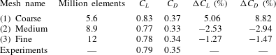
, respectively. It was found that the lift and drag coefficients obtained with the medium and the fine mesh are very close to and comparable with the experimental results; the medium mesh was within 3 % and the fine mesh within 2 % of the experimental results as presented in table 1. Therefore, the fine mesh with 12 million elements was selected as the most suitable for this study.
Mesh independence study at
 $20^{\circ }~\text{AoA}$
at
 $Re=1.83\times 10^{5}$
.

A turbulent regime simulation case was developed based on the baseline case described above. A mesh sensitivity study was conducted for the turbulent flow regime, using three meshes: 11 M, 12 M and 13 M elements, confirming that the adopted baseline set-up with fine mesh was appropriate for the turbulent flow regime.
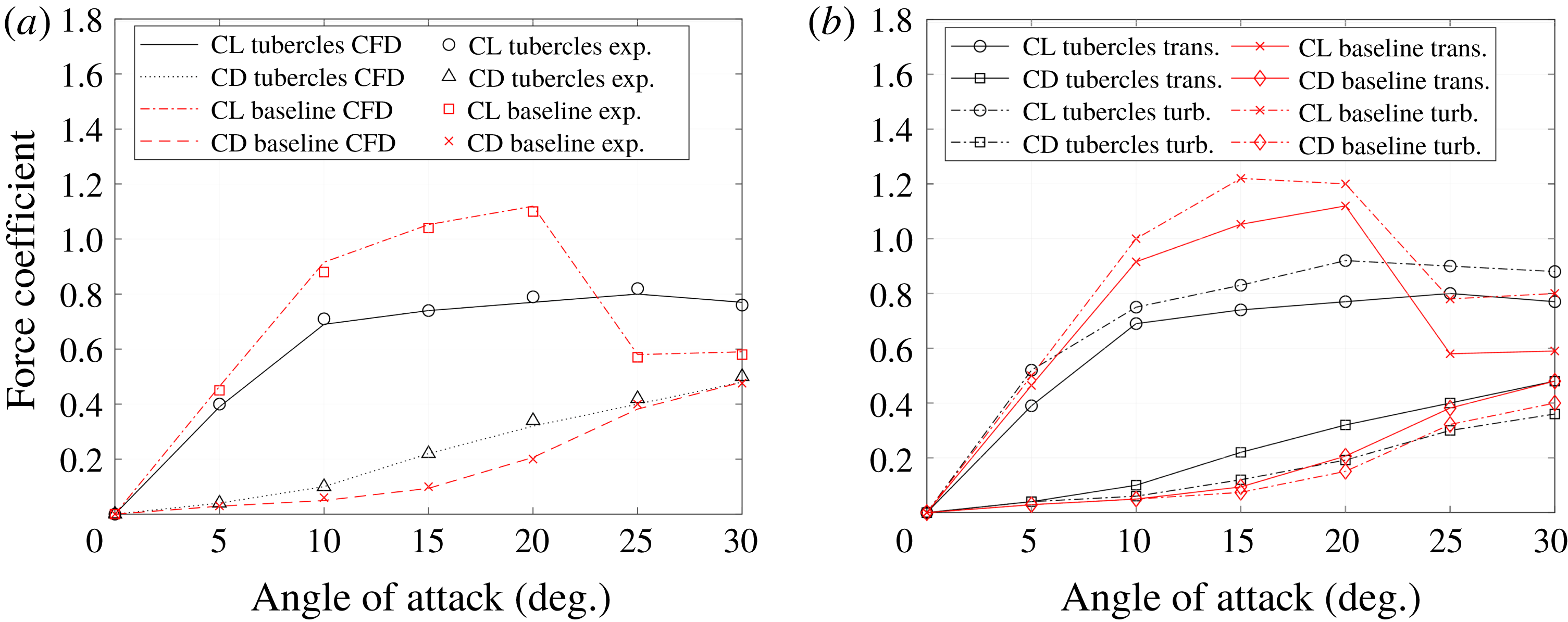
(a) Comparison of the lift and drag coefficient between CFD and experiments in the transitional regime (Johari et al. Reference Johari, Henoch, Custodio and Levshin2007). (b) Numerical result for lift and drag coefficients in the transitional and turbulent flow regime for the range of angles of attack.

5 Result analysis
5.1 Validation
Experimental lift and drag coefficients obtained by Johari et al. (Reference Johari, Henoch, Custodio and Levshin2007) were used to validate the set-up in the transitional flow regime. In figure 2(a), a comparison is shown between the experimental and numerical (CFD) lift and drag coefficients for the baseline and tubercled foils. Overall, the numerically predicted coefficients correlate very well with the experimental results in the transitional regime. The results show that for the baseline foil, the lift coefficient increases rapidly from 0 to
 $10^{\circ }~\text{AoA}$
, and steadily until
 $20^{\circ }$
, where stall occurs and
 $C_{L}$
substantially drops. When looking at the tubercled foil, it can be seen that in transitional regime at low angles of attack its behaviour is worse than the baseline foil. However, once the baseline foil reaches the stall angle, the tubercled foil is able to maintain a nearly constant lift without stall occurring.
The CFD simulations were able to catch the same trend of lift and drag curves across the range of angles of attack, with an excellent level of deviation of 2 % only. Therefore, the adopted numerical model and mesh refinement were adopted as a baseline set-up for the further study of transitional and turbulent flow.
5.2 Hydrodynamic performance
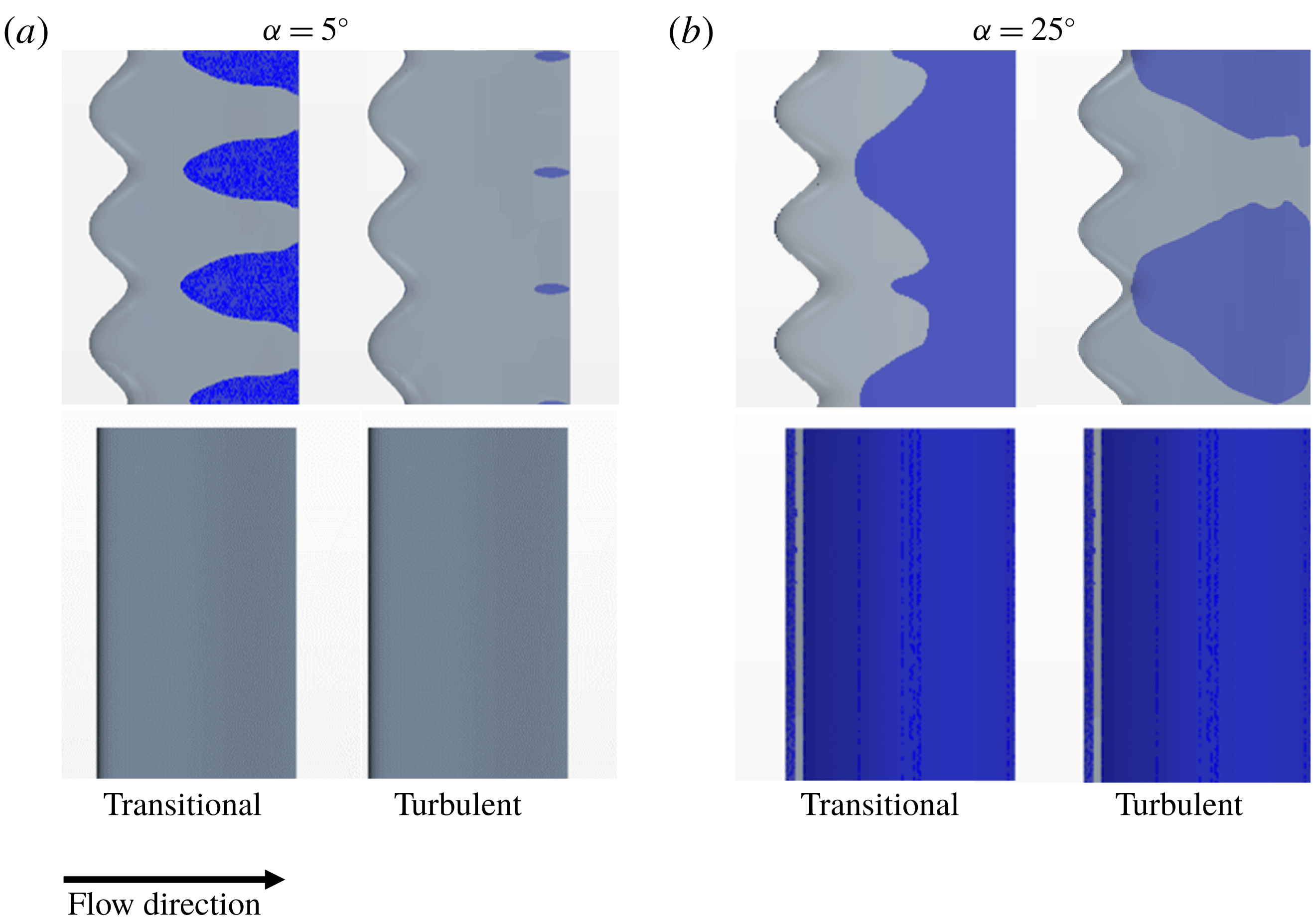
Figure 2(b) shows the calculated lift and drag coefficients for both hydrofoils, the tubercled and the baseline, comparing their performance in turbulent and transitional flow regimes. Figure 3 shows the flow separation pattern for both hydrofoils and in both flow regimes at two angles of attack,
 $5^{\circ }$
(figure 3
a: pre stall) and
 $25^{\circ }$
(figure 3
b: post stall). The regions of negative shear stress in the streamwise direction are shaded, indicating the occurrence of flow separation.
(a) Plan view of the hydrofoil suction side showing (blue) flow separation in transitional (left) and turbulent (right) flow regimes for the tubercled and baseline foils at
 $5^{\circ }~\text{AoA}$
. (b) Plan view of the hydrofoil showing (blue) flow separation in transitional (left) and turbulent (right) flow regimes for the tubercled and baseline foils at
 $25^{\circ }~\text{AoA}$
.

The coefficients for the baseline foil (figure 2
b) demonstrate similar trends in the turbulent and in the transitional flow regimes. The lift coefficient
 $C_{L}$
increases rapidly from 0 to
 $10^{\circ }~\text{AoA}$
, and steadily until
 $20^{\circ }$
, when stall occurs and
 $C_{L}$
rapidly drops. This is consistent with the flow separation captured in figure 3. At small AoA the baseline foil shows no flow separation in both regimes. However, at the post-stall AoA (
 $25^{\circ }$
), the flow on the suction side is completely separated. In regard to the drag coefficient,
 $C_{D}$
increases continuously throughout the range of AoA, with slightly lower values in the turbulent regime.
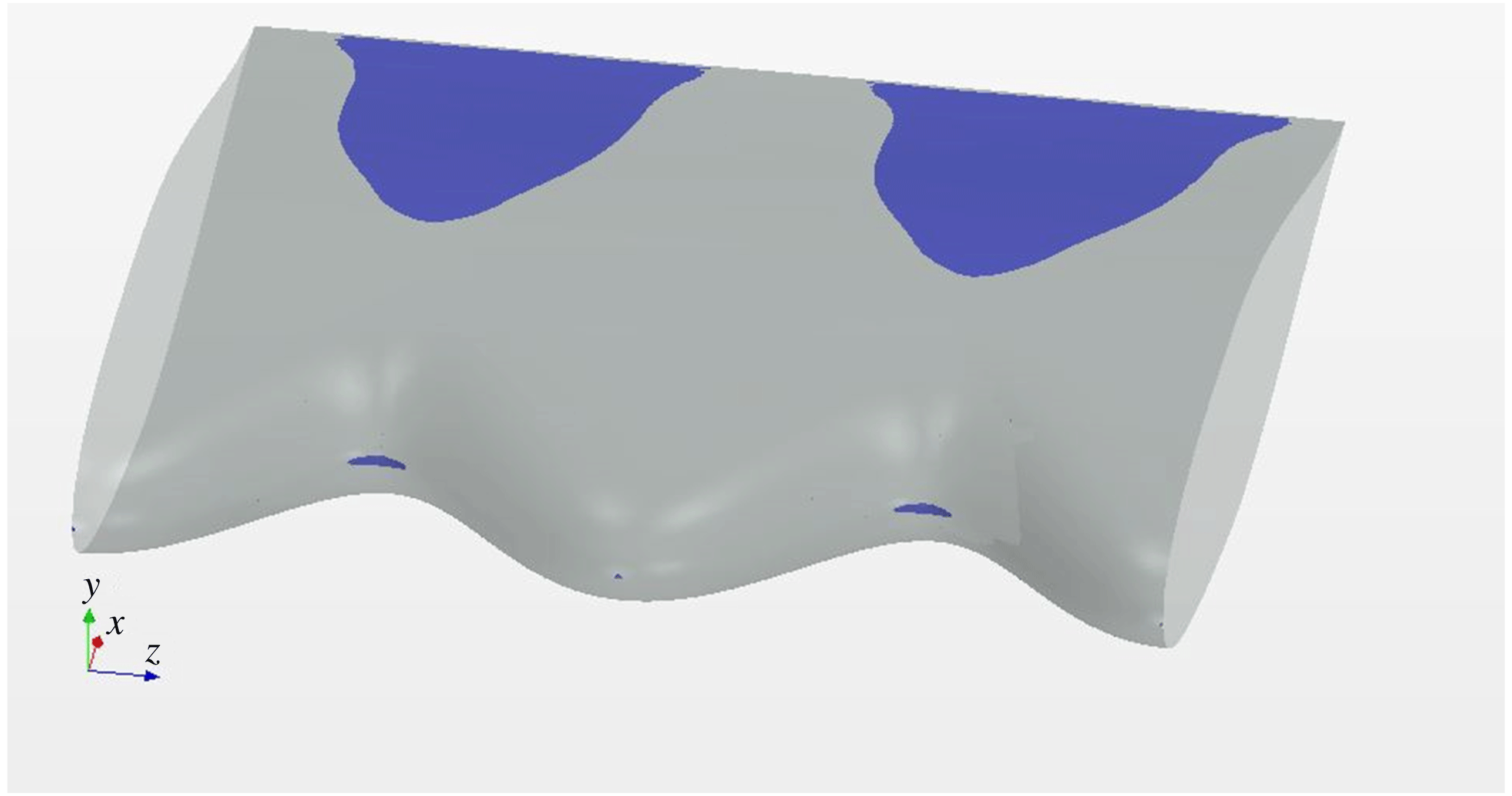
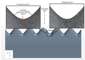
Isometric view of the foil showing the laminar separation bubble over the leading edge of the tubercled foil in the transitional regime at
 $5^{\circ }~\text{AoA}$
.

In case of the tubercled foil, the performance in transitional and turbulent flow is comparable as the curves have a similar trend, with
 $C_{L}$
and
 $C_{D}$
increasing throughout the whole range of AoA (figure 2
b). However, the performance in the turbulent regime is better than in the transitional with higher
 $C_{L}$
and lower
 $C_{D}$
through the whole range of AoA. The flow separation is present in both regimes (figure 3). At low AoA, in the transitional regime, it is observed that the separation occurs further upstream over the troughs rather than over the peaks (at around
 $1/3$
of the chord). This is consistent with the findings in the literature (Miklosovic et al.
Reference Miklosovic, Murray, Howle and Fish2004; Hansen Reference Hansen2012; Rostamzadeh et al.
Reference Rostamzadeh, Hansen, Kelso and Dally2014; Bolzon, Kelso & Arjomandi Reference Bolzon, Kelso and Arjomandi2015). Additionally, a laminar separation bubble is identified at the leading edge of the troughs in the transitional flow regime (as shown at the isometric view in figure 4). Figure 3 shows that the level of flow separation on the suction side is lower in turbulent flow than in transitional for the whole range of AoA. At low AoA, the difference between the scale of the separation in the transitional and turbulent flow is obvious. While in transitional flow significant areas of separation were identified behind each trough and developing further downstream, in turbulent flow the separation is identified only in a very small region close to the trailing edge and further downstream. This confirms that in turbulent flow the separation is significantly suppressed and shifted further downstream compared with transitional flow. At high AoA, the flow separation is high, however still below the level captured in the transitional flow regime.
When comparing the performance in the turbulent regime of the tubercled foil with the baseline one, it can be seen that at low angles of attack the tubercled foil behaviour is worse than the baseline foil (lower
 $C_{L}$
and higher
 $C_{D}$
). However, once the baseline foil reaches the stall angle and experiences a drop in
 $C_{L}$
(around
 $20^{\circ }$
), the performance of the tubercled foil becomes superior as it is able to maintain
 $C_{L}$
at approximately the same value while
 $C_{D}$
is slightly reduced. This lower drag coefficient at large AoA is not achieved in the transitional regime and is only specific for behaviour in the turbulent flow regime.
In line with the results presented in figures 2 and 3, in can be concluded that in both regimes at pre-stall AoA, the baseline foil performs better than the tubercled foil as flow separation does not occur. In contrast, at post-stall AoA, the tubercled foil performance is superior as the level of flow separation is lower than for the baseline foil where the flow separation occurs across a whole suction side.
5.3 Tubercle mechanisms of action
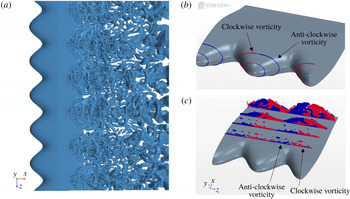
This study confirmed that the fundamental leading edge tubercle mechanism of action that researchers encountered in the transitional and laminar flow regime is present in the turbulent flow regime as well. The first feature is the existence of a three-dimensional (3-D) streamwise counter-rotating pair of vortices formed over each tubercle peak. These vortex structures are confirmed by positive isosurfaces of the
 $Q$
criterion
 $Q_{}={\textstyle \frac{1}{2}}(\unicode[STIX]{x1D6FA}_{ij}\unicode[STIX]{x1D6FA}_{ij}-\unicode[STIX]{x1D61A}_{ij}\unicode[STIX]{x1D61A}_{ij})^{1/2}$
, where
 $\unicode[STIX]{x1D734}$
is the rotation tensor and
 $\unicode[STIX]{x1D64E}$
is the strain tensor (Hussain & Jeong Reference Hussain and Jeong1995). The identified 3-D vortices are shown in figure 5(a) and are generated due to the difference in pressure that exists between the pressure and suction faces of a hydrofoil’s peaks. They are created due to the flow’s tendency to travel from the high pressure to the low pressure regions of the hydrofoil (figure 5
b). The size of the counter-rotating vortices gradually increases, mixing the upper regions of the boundary layer, as shown in figure 5(c). This phenomenon is seen at all angles of attack, being weaker at lower angles of attack as expected and it is consistent with the literature (Rostamzadeh et al.
Reference Rostamzadeh, Hansen, Kelso and Dally2014; Skillen et al.
Reference Skillen, Revell, Pinelli, Piomelli and Favier2015).
(a) Instantaneous isosurfaces of
 $Q$
criterion; (b) and (c) evolution of the streamwise vorticity at different chord locations at
 $10^{\circ }~\text{AoA}$
in turbulent regime.

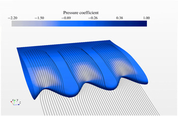
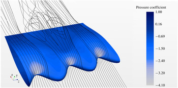
The second feature observed in the turbulent regime is a cyclic variation of the pressure in the spanwise direction, resulting in the depression areas behind the troughs on the suction side of the hydrofoil (figures 6 and 7). These pockets of low pressure (white regions) direct the fluid particles to move transversally from the zones of high pressure (peaks) to the zones of low pressure (troughs), leading to the formation of a secondary spanwise flow. As shown in figure 6, this is manifested by the near-wall streamlines being squeezed from the peaks towards the troughs. This finding is seen at low angles (figure 6) and high angles (figure 7) of attack and it is consistent with the observations in the transitional and laminar flow regimes (Rostamzadeh et al. Reference Rostamzadeh, Hansen, Kelso and Dally2014, Reference Rostamzadeh, Kelso and Dally2017; Skillen et al. 2014). Due to this secondary flow, the low momentum fluid particles that lie next to the wall are deflected and transported away from the peaks towards the troughs (Skillen et al. Reference Skillen, Revell, Pinelli, Piomelli and Favier2015). The near-wall region over the peaks (figures 6 and 7: see the gap between streamlines pattern) is filled with higher momentum fluid that is transported down from the upper region of the boundary layer, explaining why the first occurrence of separation is located behind the troughs (figure 3).
Suction side pressure distribution and near-wall time-averaged streamlines in turbulent flow at
 $5^{\circ }~\text{AoA}$
.

Suction side pressure distribution and near-wall streamlines in turbulent flow at
 $25^{\circ }~\text{AoA}$
.

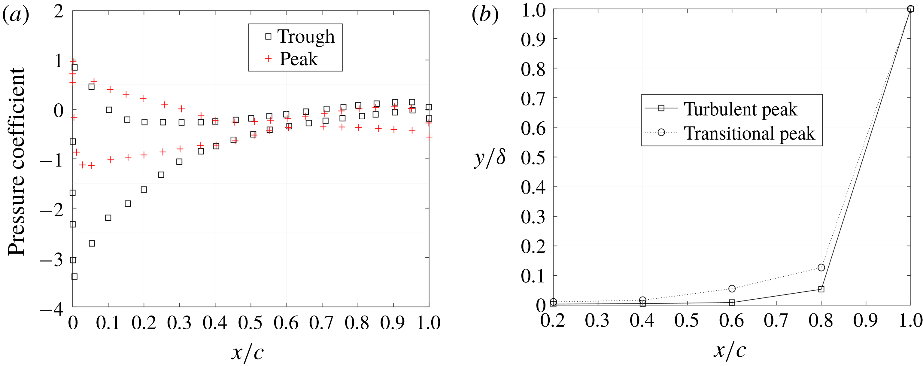
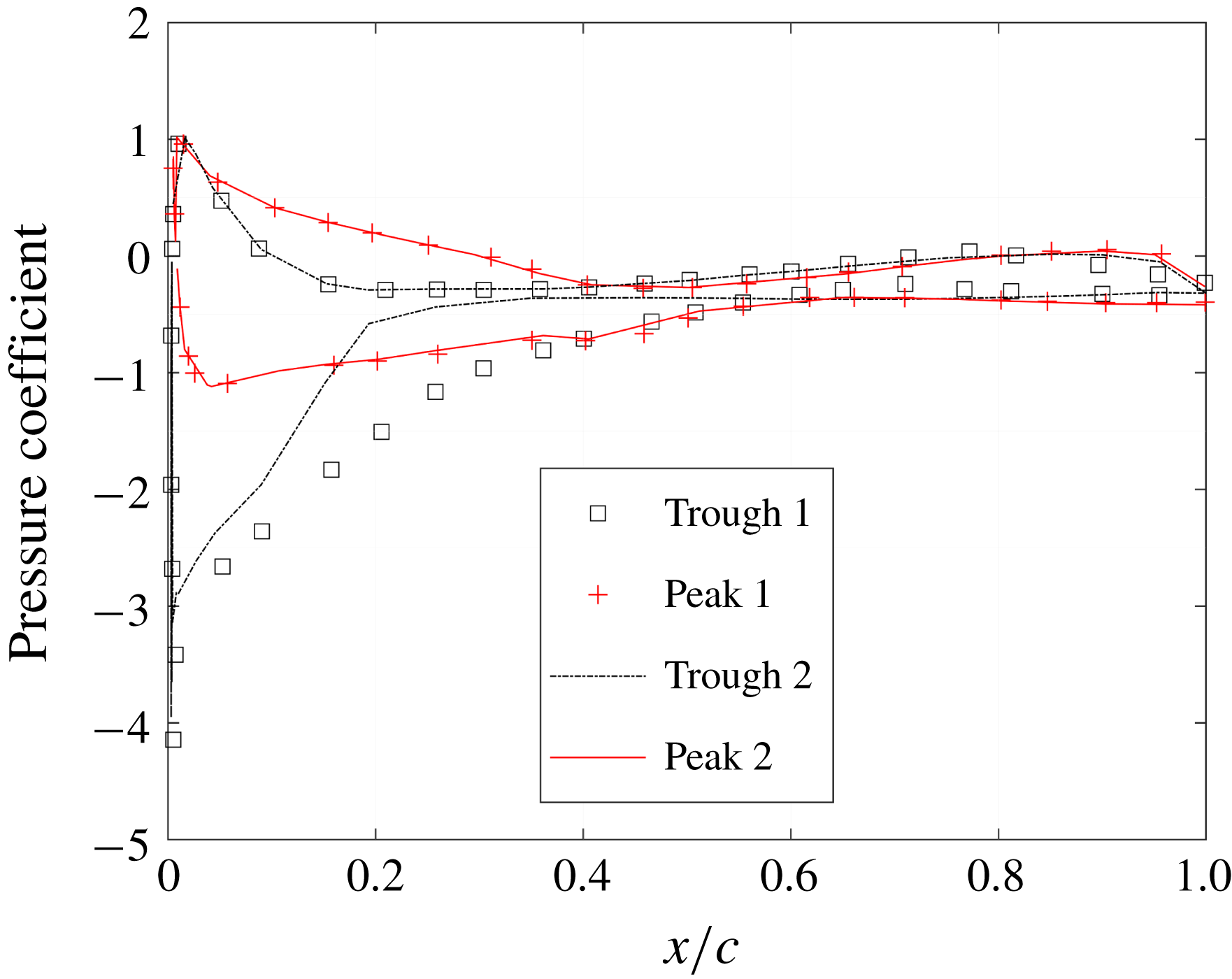
The existence of the minimum pressure at the troughs and spanwise pressure differences as shown in figure 6 is also confirmed by the pressure distribution along the chord (presented in figure 8 a). These two curves are measured at the centre-most peak and trough. Small spanwise pressure variations of within 1 %–2 % are measured at low AoA. High AoA pressure distribution over the two sets of peaks and troughs shown in figure 7 are presented in figure 9. From the pressure distribution it is clear that consecutive troughs present a different pressure distribution along the suction side of the hydrofoil. This is due to vortex interactions or the ‘bi-periodic phenomenon’ already reported in experiments (Johari et al. Reference Johari, Henoch, Custodio and Levshin2007) and numerical studies (Zhao et al. Reference Zhao, Zhang and Xu2017).
(a) Pressure distribution along the chord at
 $10^{\circ }~\text{AoA}$
in the turbulent flow regime. (b) Peak’s boundary layer thickness on different locations along the chord at
 $10^{\circ }~\text{AoA}$
.

In addition, figure 8(a) shows a spanwise variation of the pressure at all angles of attack, the minimum pressure is developed over the suction side troughs. The same phenomenon is identified in the laminar and transitional flow regimes and is consistent with the literature (Hansen Reference Hansen2012). This pressure variation is caused by the difference in chord lengths at peaks and troughs together with the curved shape of the foil that drives the vortices to migrate towards the trough and form low pressure regions. As a consequence, the bulk of the flow is directed behind the chord minima (troughs). As a consequence, strong flow acceleration behind the troughs causes a local augmentation of the minimum suction pressure (Skillen et al. Reference Skillen, Revell, Pinelli, Piomelli and Favier2015).
Pressure distribution along the chord at
 $25^{\circ }~\text{AoA}$
in the turbulent flow regime.

This flow pattern causes changes in the boundary layer as well. Figure 8(b) presents the boundary layer thickness along the peak’s chord for transitional and turbulent flow. As expected, with an increase in Reynolds number the boundary layer becomes thinner. This difference in the thickness of the boundary layers has been seen across the whole range of angles of attack under consideration.
For the tubercled foil, this thinning phenomenon is more pronounced due to a combination of the mixing mechanism as part of the vortex generation and second mechanism of influx of the higher momentum fluid particles from the upper region of the boundary layer into the near-wall region. This phenomenon does not conflict with the control mechanisms of action of the tubercled foil. Instead, it amplifies the generation of the large 3-D vortices, improving the hydrodynamic performance of the hydrofoil overall.
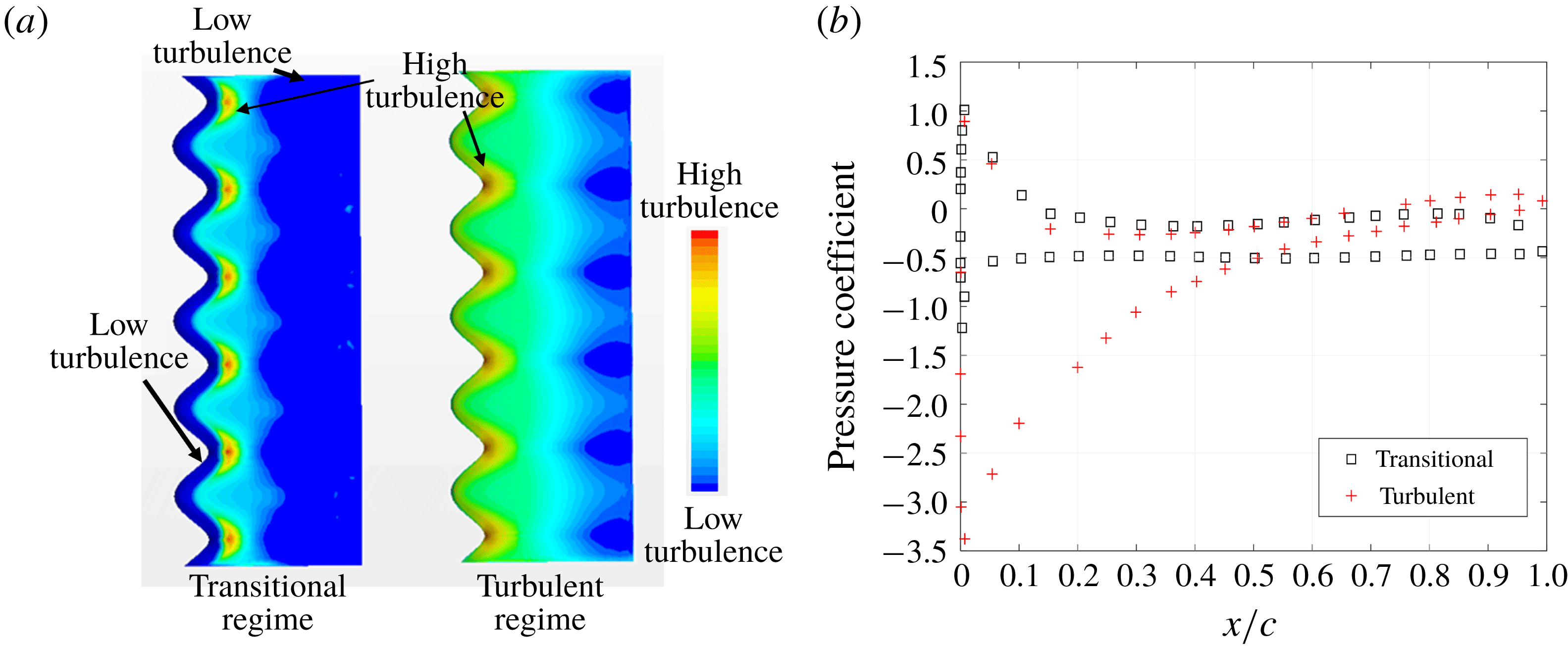
Turbulent kinetic energy on the suction side at
 $10^{\circ }~\text{AoA}$
. (b) Trough pressure distribution at
 $10^{\circ }~\text{AoA}$
in turbulent and transitional flow regime.

5.4 Development of turbulence
Figure 10(a) shows a turbulent kinetic energy (
 $k$
) field in the near-wall region for the transitional and turbulent flow regimes. The regions coloured in blue (dark and light) indicate the zones of low turbulence where the flow is mostly laminar, whereas regions coloured in yellow and red indicate the zones where the turbulent flow is developing. In transitional flow regimes, there is a small region along the leading edge that sees a laminar flow (dark blue region) before the transition to turbulent flow takes place, followed further downstream by flow separation (blue region again). In contrast, in the turbulent regime, the turbulent boundary layer is energised further upstream than in the transitional flow regime and a high turbulent kinetic energy is seen immediately behind the troughs, near the wall. This is caused by the high velocity gradients that are formed as the near-wall flow moves from the peak to the trough. This explains why the hydrofoil in the turbulent flow regime experiences less flow detachment.
Another observation that explains why the troughs experience less detachment in the turbulent flow regime can be made from the pressure distribution presented in figure 10(b). In the transitional flow regime, the pressure on the leading edge of the suction side increases instantly while in turbulent flow regime, the pressure increases gradually. As a result, in the transitional flow regime laminar separation bubbles are formed at the leading edge on troughs, whereas in the turbulent flow regime, the formation of the separation bubble is suppressed together with its detrimental effects (drag and separation). This is further confirmed by the wall shear stress distribution on the suction side of the foil shown in figure 11. In the transitional flow regime, near the leading edge, the region of the laminar separation bubble is identified (left-hand inset) whereas right-hand inset shows that, in the turbulent flow regime, the laminar separation bubble does not exist. This is an important finding, not previously reported in the literature, that extends our understanding of the turbercled foil performance in turbulent flow.
Shear stress plotted using the line integral convolution technique at
 $5^{\circ }~\text{AoA}$
for transitional and turbulent flow regimes.

6 Conclusions
This research confirms that the behaviour of turbercled hydrofoils in the turbulent flow regime is consistent with phenomena identified in the transitional flow regime for an incompressible fluid. When comparing a turbercled and a smooth baseline hydrofoil, analysis confirmed that, at pre-stall angles of attack, the baseline hydrofoil performs better than the tubercled in all turbulent and transitional flow regimes. However, in post-stall conditions, when the baseline performance suddenly drops, the tubercled foil becomes superior due to the lower level of flow separation, increased lift and lower drag coefficients.
The main mechanism of action of a tubercled hydrofoil in the turbulent flow is the formation of pairs of counter-rotating streamwise vortices mixing a near-wall low momentum flow with a higher momentum flow from the upper region of the boundary layer. This phenomenon is combined with the appearance of the secondary flow in a spanwise direction caused by the pressure difference behind peaks and troughs. In the turbulent flow regime, at lower angles of attack the flow separation on the suction side is significantly suppressed, as well as the laminar separation bubble that, in the transitional flow regime, exists on the leading edge of troughs. In addition, for the tubercled hydrofoil in the turbulent flow regime, the study identified a phenomenon of thinning of the boundary layer that takes place, further delaying the stall. This phenomenon does not conflict with the principal tubercle mechanism of action. On the contrary, it contributes to more stable mixing of the vortices and improves the overall hydrodynamic performance of the foil.
This numerical modelling approach that is able to capture the tubercled hydrofoil action in sufficient detail is recommended as part of a systematic analysis of tubercled hydrofoil devices and their design. This is of significant importance when looking at potential application on ships as it would replace the commonly used practice where expensive physical testing is needed to assess the ship’s performance and identify further design iterations required.
The importance of this study is that it gives in-depth insight into the complex mechanism of action of the tubercled hydrofoil over the whole range of flow regimes and angles of attack. This work contributes to the knowledge required to investigate the potential applications of tubercles as hydrodynamic flow control devices.
As a future work, it would be beneficial to confirm the findings presented in this paper with a comprehensive experimental investigation of the tubercled hydrofoil in an incompressible, fully turbulent flow regime. In addition, it is recommended to investigate how the tubercles’ geometric parameters impact the thinning of the boundary layer and 3-D vortex generation phenomena. These further works would allow us to better predict and control flow behaviour and identify potential future flow control technology applications.