SAMPLE SELECTION BIAS AS AN ECONOMIC AND HISTORICAL ISSUE

Sample-selection bias is a potential problem for every source that was not produced or collected for the entire population, or for which only non-random sub-samples survive. Selection bias also affects textual and other non-quantitative sources. A document’s survival to the present, for example, may indicate that its author differed from others creating similar documents at the same time. These issues often present themselves in the study of economic history. Yet, economic historians cannot dispense with the use of surviving, sometimes nonrandom, samples; and we do not advocate that they do. Rather, we stress a theoretical and econometric version of an old practice among historians: ask hard questions about potential source bias.

Modern econometric techniques for dealing with sample selection bias arose out of efforts to study the wages and labor supply of married women. Many married women do not work in the formal labor market, so surveys cannot report their potential earnings; but to understand women’s labor-supply decisions, researchers need to know what a woman would earn, had she chosen to work in the labor market. If there are unobserved factors that affect both potential wages and employment decisions, we cannot infer the potential wages of non-working women from a sample of working women, even if we use controls to construct apparent like-to-like comparisons (Gronau Reference Gronau1974; Heckman Reference Heckman1979). Regression models cannot uncover consistent estimators of the determinants of potential wage offers from information on observed wages. This is a form of selection on unobservables: unobserved factors may imply that working women might earn more or less than observationally identical, non-working women had they instead entered the workforce. Working women may differ in other, observable ways, as well, but this selection on observables can be dealt with using regression or weighting techniques.^{Footnote 1}

Heights researchers using certain types of samples face a problem similar to that faced by students of labor supply: the sample consists only of those who have made a choice that led to their inclusion in the sample. The decision to join the military, for example, may be driven by unobservable traits not recorded in the data, but correlated with height. To the extent the literature concerns itself with sampling issues, it generally focuses on selection on observables. Military samples, for example, may include enlistees drawn disproportionately from a specific occupation or social class. This type of selection poses only trivial challenges for researchers, who can obtain valid population estimates by controlling for occupation or social class in a regression, or by re-weighting the sample to reflect the proportions of that class in the population as a whole. Selection on unobservables poses a different challenge: the weights necessary to construct a valid representation of the population are unknown, because they depend, in part, on relationships among unobservables. Oversampling on observable traits does not bias conditional estimates of average height. Bias arises when the laborers in the sample (for example) are shorter or taller than laborers in the population as a whole due to unobservable factors that lead to their inclusion in the sample.

Sample selection bias means that we cannot know whether the sample mean height equals the population mean height without knowing the process that selected the sample from the population. Selection bias also means we cannot make confident statements about the relationship between population mean height and any individual trait. For this reason and despite assertions to the contrary, sample-selection vexes crosssection studies (Squicciarini and Voigtländer Reference Squicciarini and Voigtländer2015).

Drawing inferences about trends from a time-series of height data subject to selection bias will create even greater challenges to drawing inferences if selection on unobservables changes over time or with age at observation. Komlos and A’Hearn (Reference Komlos2019, p. 1137) assume this problem away when they assert that selection operated equally across cohorts, which may yield biased estimates of cohort coefficients, but still allow them to capture a true trend. There are two facts about the antebellum economy that render this assumption untenable: (1) a sharp cyclical downturn between 1837 and 1843 followed by a long expansion to the late 1850s; and (2), as Komlos (Reference Komlos2019) reminds us, the antebellum economy experienced unprecedented changes by way of innovations in manufacturing and transportation, urbanization, immigration, and internal migration. Returning to our female labor force participation analogy, it would be hard to argue that women’s selection into the U.S. labor force remained time-invariant between 1975 and 2010 when the fraction of married women in the labor force increased by 20 percentage points. It is equally difficult, to us at least, to assert time-invariant selection into militaries, prisons, universities, manumissions or the slave trade in the face of such wide-ranging transformations that remade the antebellum economy.

To support their contention that selection bias is and has been acknowledged and accounted for in the literature nearly from its inception, Komlos and A’Hearn (Reference Komlos2019, p. 1135) cite Margo and Steckel (Reference Margo and Richard1983) as an early recognition of selection bias that continues to inform the literature. After finding that farmers and white-collar workers who joined the Union Army were taller than common laborers, Margo and Steckel (Reference Margo and Richard1983, p. 172) discuss the possibility of unobserved height-based selection into farming and white-collar occupations. They do not explore the possibility or the implications of unobserved height-based selection into the military sample they analyze even though they earlier noted the declining heights of recruits as the war ground on. Finding that late-war recruits were nearly an inch shorter, after controlling for observables, than early-war recruits and speculating that this fact may be due to “interaction effects or variables not included in the regression” (Margo and Steckel Reference Margo and Richard1983, p. 172) is not what we consider an acknowledgment and accounting for selection on unobservables. To their credit, Margo and Steckel conclude this discussion with the observation that the issue “remains a subject for future research” (ibid, p. 172). The few studies that make up this “future research” pale in volume to the hundreds of studies of selected samples that rarely acknowledge the issue.

Komlos and A’Hearn then point to Zimran (Reference Zimran2019), who asks whether sample-selection bias affects the Union Army data’s ability to speak to an antebellum puzzle, as evidence that even if choice-based samples are subject to selection bias, the resulting bias is small. Zimran first links Union Army soldiers to their entries in the census, and then uses a Heckman-style (Reference Heckman1979) control-function model to address the adjustment to cohort height implied by the selection corrections. We have two reservations about Zimran’s approach that leave us less than fully convinced by his results. First, the linkage creates a second potential selection-bias problem. Bailey et al. (Reference Bailey, Cole, Henderson and Massey2017) show that machine-matching algorithms introduce the possibility of type-I errors (false positive matches) and, more importantly in low-match-rate environments, type-II error (no matches), both of which complicate inference in regressions on linked data sets. The unmatched may represent, to some extent, selection on observables, but there is enough possible selection on unobservables that the linkage raises serious questions. Second, Zimran attempts to control for selection using a single-index model and, as his identifying instrument, the share of the Republican vote by soldier’s county of residence in 1860, a proxy for commitment to the cause, or “patriotism.” With multiple types of selection—selection into the Army at different ages and selection in matching Army and census records—a single-index model is incorrect (Tunali Reference Tunali and Ehrenberg1986; Schmertmann Reference Schmertmann1994; Vella Reference Vella1998).^{Footnote 2} We agree with Zimran that selection needs to be modeled with care. We do not think his approach, as currently formulated, solves the problem inherent to this literature, however.

DIAGNOSING SAMPLE-SELECTION BIAS IN CHOICE-BASED SAMPLES

Komlos and A’Hearn also question the way we implement the diagnostic for sample selection bias that we develop elsewhere (Bodenhorn, Guinnane, and Mroz Reference Bodenhorn, Timothy, Thomas, Wolcott and Hanes2019b) and apply in our 2017 article. We report results for four different samples, although Komlos and A’Hearn focus on our results for the Union Army alone. The diagnostic works off internal evidence of selection on unobservables; a more straightforward test would compare a selected sample to either a random sample or the population. The non-selected sample is of course not available in this instance. We believe Komlos and A’Hearn explain and apply our diagnostic correctly. We differ in our views on its relationship to earlier research on heights as well as the diagnostic’s implications.

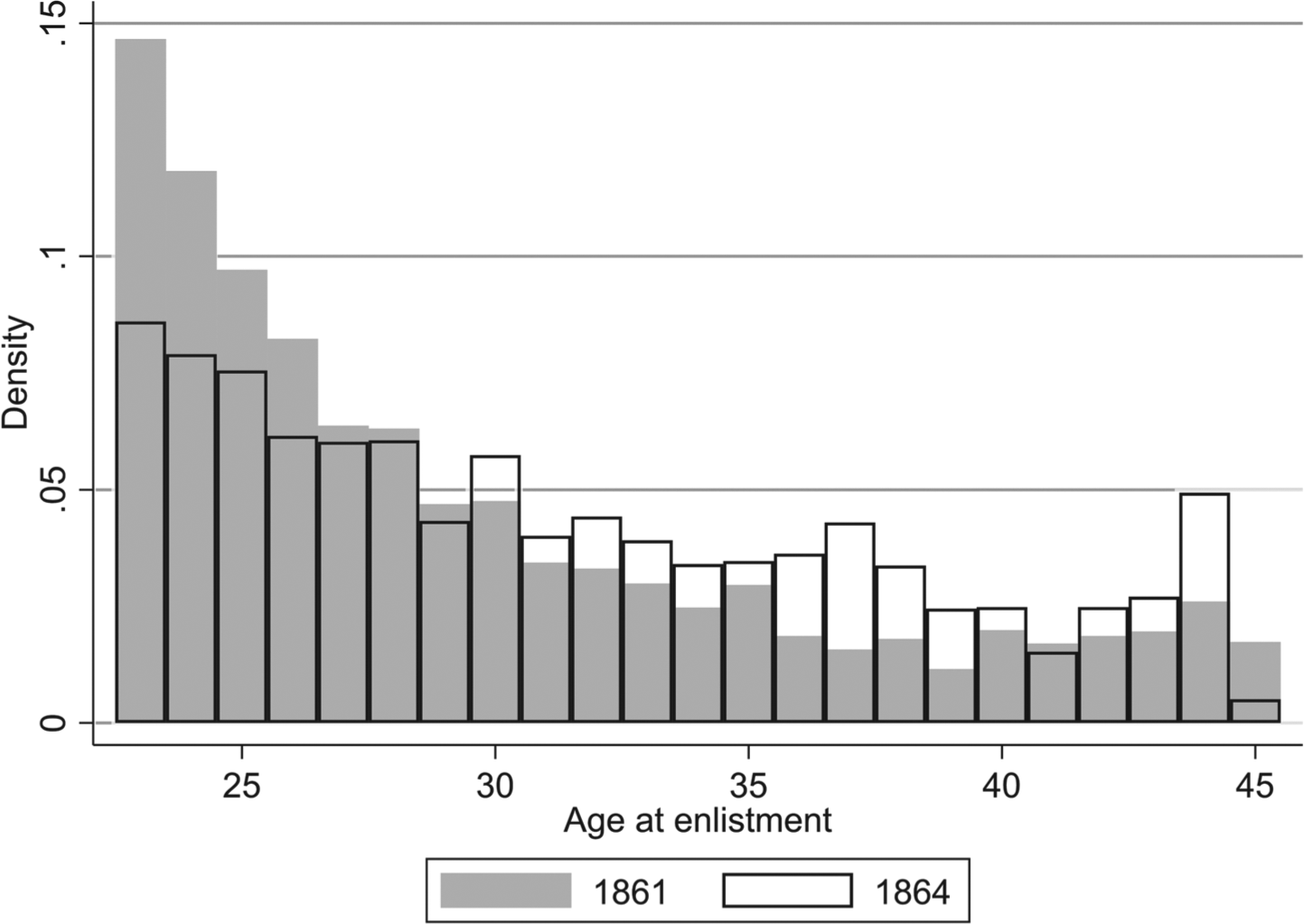
Komlos and A’Hearn agree with us that there is abundant evidence of sample-selection bias in the Union Army data (Fogel et al. Reference Fogel, Dora, Haines, Lee, Nguyen, Pope, Rosenberg, Scrimshaw, Trussell, Sven Wilson, Wimmer, Bassett, Burton and Yetter2000). They actually present additional evidence that reinforces our point. They note that the distribution of age at enlistment varied considerably across enlistment years. Figure 1 reports histograms of the age at enlistment for those enlisting in 1861 and in 1864. ^{Footnote 3} The two distributions are clearly unequal (Kolmogorov-Smirnov test, p < 0.001). Older recruits were scarce, yet as the war dragged on the median age at enlistment rose by three years between 1861 and 1864. The paucity of older recruits and the changing age composition of enlistees over time, raises questions about why individuals enlisted at different ages and how that reflected their economic circumstances. Komlos and A’Hearn’s Figure 5 and Online Appendix Figures A1 and A2 provides more direct evidence of sample-selection by economic circumstances. From the war’s start, the Union Army’s soldiers were poorer than average northern white males. This wealth gap increased with the soldier’s age. At age 30, the average Union Army recruit had about half as much wealth as the average northern white male. By age 40, the new recruits had one-third as much wealth (Komlos and A’Hearn Reference Komlos2019, figure 5).

Figure 1

DISTRIBUTION OF AGES AT ENLISTMENT, BY YEAR OF ENLISTMENT

Notes: The distributions of ages at enlistment come from Union Army Data (Fogel et al. Reference Fogel, Dora, Haines, Lee, Nguyen, Pope, Rosenberg, Scrimshaw, Trussell, Sven Wilson, Wimmer, Bassett, Burton and Yetter2000), only for those born in the United States and who enlisted from ages 23 to 45. Birthplace came from the variable “rb_stat1.” The variable “lstag1_1” provided the information on age at enlistment, and the variable “lstdt1_1” provided information on date of enlistment.

Sources: Authors’ calculations from Union Army Data (Fogel et al. Reference Fogel, Dora, Haines, Lee, Nguyen, Pope, Rosenberg, Scrimshaw, Trussell, Sven Wilson, Wimmer, Bassett, Burton and Yetter2000).

These facts, as well as the rapidly evolving antebellum economy, inform our prior that the Union Army does not constitute a random sample of the male population. Some of the prior evidence discussed earlier is external to the army data, but we now turn to our selection diagnostic, which identifies selection from internal evidence. Our diagnostic works by searching for patterns in the selected sample that would not be present in the absence of height-based selection. The logic is as follows. Consider a group of men born in 1835 who joined the Union Army in various years: 1860, 1861, etc. Men born in 1835 who joined in 1860 should not be systematically shorter or taller than those who joined in 1861. If they are, we have evidence that some change in either the attractiveness of military service or the civilian alternatives led to different types of men joining in 1861 than those that joined in 1860. This is selection bias. Because we have men who joined the Union Army and were born in several different years, we can also consider interactions of birth year and age-at-recruitment (or, equivalently, year-of-recruitment) effects. These interactions allow for changes in selection bias over time picked up by the age-at-enlistment dummies. We estimate the regression:

$${h_i} = \mathop \sum \nolimits_{j = 1}^N {\beta _j}{B_j} + \,\mathop \sum \nolimits_{j = 1}^m {\alpha _j}{A_j} + \mathop \sum \nolimits_j^N \sum\nolimits_K^M {{\delta _{jk}}{B_{jk}}{A_k} + {\varepsilon _{i,}}}$$

where h represents height, the Bs are dummies for birth year, and the As are dummies for age at enlistment. ^{Footnote 4} Under the null hypothesis of no height-based selection, we would interpret the βs as measuring the trend in mean heights. If heights within a birth cohort do not differ across recruitment ages, then the αs and δs are zero. If this height-based selection does not change across birth-cohorts, then the δs are zero. The diagnostic boils down to one or more χ ² tests for the null hypothesis that the as and the δs are collectively zero. Our 2017 article (Tables 5 and 6) reports this diagnostic test for the Union Army, the British Army, and samples of Pennsylvania prisoners and free African-Americans in the Chesapeake region. In most cases we find evidence of selection that differs by age and cohort.

Komlos and A’Hearn accurately describe the diagnostic and their results. But we disagree with their interpretation in three ways. First, they interpret Equation (1) as correcting for selection bias. It cannot, and we are clear about that fact. There is an important difference between a diagnostic and a correction. At several points, they refer to “controlling” for selection bias and incorrectly interpret our econometric approach as efforts to report trends in mean height unaffected by selection bias. Komlos and A’Hearn (2019, p. 1135) write: “… there was increasingly negative selection on height during the war. So long as this operated equally, within a given enlistment-year, on men of all birth-years, controlling for enlistment-year allows us to estimate the time trend in heights accurately. This has been the standard practice.” This statement is incorrect. The age-at-recruitment dummies should be zero if there is no height-based selection. But including those dummies in the regression does not “control” for selection, as we demonstrate later. Komlos and A’Hearn’s discussion of and disagreement with our analysis of the regression approach betrays a fundamental confusion of selection on observables and selection on unobservables. Sample-selection bias in Heckman’s (Reference Heckman1979) sense is about unobservables. One cannot “control for” an unobservable using a variable, which by definition is observable, without imposing strong assumptions like those detailed in the next section that describe how unobservables in the selection process are related to height.

Yet several studies, including studies by Komlos (Reference Komlos, Komlos and Baten1998b) and A’Hearn (Reference A’Hearn, Komlos and Baten1998), include enlistment year effects in height regressions on Union Army soldiers. They, and Haines (Reference Haines, Komlos and Baten1998), Cuff (Reference Cuff, Komlos and Baten1998), and Craig and Weiss (Reference Craig, Weiss, Komlos and Baten1998) all report statistically significant enlistment-year effects, although the magnitudes vary with the particular subsample used. Only Komlos (Reference Komlos, Komlos and Baten1998b, p. 242) goes beyond a simple discussion of the result: he writes “the decline in heights between the 1864 and 1865 recruitment years was caused by some particularities of the recruitment procedure in the last year of the war, and was not a birth cohort effect.” Again, he has made our point for us. Some sort of selection on unobservables led to declines in the mean heights of recruits entering the sample as the war ground on. Absent this selection, the enlistment effects would be individually and jointly zero.

Their claim that “this has been the standard practice” (p. 1135) is also misleading. Although the five studies discussed in the previous paragraph include year-of-enlistment dummies, our reading of nearly 150 height studies did not uncover any studies of prisoners, students, or others that include age-at-observation or year-of-observation dummies with or without interaction terms. It is standard practice in studies that include youths to include age-at-observation dummies for those younger than 22 years. The coefficients on these dummies are interpreted strictly as the effect of an additional year of the adolescent growth spurt alone on height when they may, in fact, be indicative of selection effects among young enlistees, criminals, students, and manumitted slaves.

Our 2017 regression results, Komlos and A’Hearn’s regression results, and the results of our simulation results (discussed later and in Bodenhorn, Guinnane, and Mroz Reference Bodenhorn, Timothy, Thomas, Wolcott and Hanes2019b) accord with the view Komlos (Reference Komlos2004) advanced in a footnote in an earlier article, where he argues strongly against controlling for year of recruitment in analyses of height samples. The issues he raises, in our opinion, cut to the heart of the matter and deserve to be addressed more prominently than in a footnote:

Komlos’s (Reference Komlos2004) statement is entirely correct: the year in which one enlists does not determine height. If age at enlistment appears to affect height in the sample, that is evidence of height-based selection. This is precisely the diagnostic’s logic. Our first and principal disagreement with Komlos and A’Hearn is whether the inclusion or exclusion of enlistment-year (or observation-year effects, more generally) effects in a regression can correct for selection bias. Including them in a regression neither solves the problem nor identifies a true trend. The simulation results discussed later show how their inclusion can reflect dynamic selection issues (age-based) that contaminate the interpretation of true population height trends.

Second, we have reservations about Komlos and A’Hearn’s discussion of the interaction terms (δs). Non-zero δs imply changing patterns of height-based selection. We report three different specifications for the Union Army. The dataset contains two different age-at-enlistment reports for each recruit, and in about 75 percent of cases, the two different reports do not agree. ^{Footnote 5} The χ ² statistic for one specification has a p-value of 0.008, but Komlos and A’Hearn dismiss this result as based on the wrong age reports. It is important to consider the purpose of the tests we report. The p-values for the other two definitions we use are about 0.166.

If we had no internal and external evidence of sample-selection bias, we would probably agree with the usual interpretation of this p-value; there is a one-in-six probability of obtaining the result by chance. This is the correct approach when one firmly believes the null hypothesis of no unobservable selection: reject the null only if the data strongly say to do so. The age-at-enlistment dummies would still demonstrate height-based selection, but the interaction terms suggest the age patterns did not differ across birth cohorts. In the current case, however, the one-in-six chance seems the wrong interpretation. We actually do not believe the null hypothesis of unchanging age patterns (time- or age-invariant selection), because most of the additional evidence, from the age and wealth selection effects observed for the Union Army to the compelling evidence of nonhomogeneous selection in other samples examined in Bodenhorn, Guinnane, and Mroz (Reference Bodenhorn, Timothy and Thomas2017), all point to time-and age-varying selection bias. Given that additional evidence, a one-in-six chance of a random result should be enough to reject the null.

It should also be kept in mind that our argument is not limited to uncovering selection in the Union Army sample alone; the results we report in our 2017 paper provide evidence of selection into the British Army, Pennsylvania’s nineteenth-century prisons, and Virginia’s free black samples. Selection, we reiterate, is endemic to nonrandom anthropometric samples.

Third, in constructing Figure 3 in our 2017 article, we use 1865 as the reference enlistment year. Komlos and A’Hearn note, correctly, that shifting the reference year to 1864 produces different predicted effects, an observation that leads them to make two different claims. They are correct that the predicted values of the dependent variable should not depend on choice of reference dummies in a linear model; in fact, they do not. The choice does, however, affect the estimated βs for the birth cohort effects, a point they stress. This is just another way of noting that the diagnostic cannot correct for selection bias. In fact, it is entirely possible to produce different implied trends in mean heights from the same regression using different enlistment years as the omitted category. This fact is a general feature of interaction terms, and not specific to our diagnostic. Again, this shows that the regression model diagnoses but does not control for selection bias.⁶ With an adequate control function to contend with sample-selection bias, the choice of reference age at enlistment would not matter. Absent an appropriate control function, it does. This is our point.

SAMPLE-SELECTION BIAS AS A SPECIFICATION ERROR

In this section we provide a straight-forward econometric derivation of the identification problem that bedevils samples subject to changing selection bias. Assume that the population regression of interest is h_i = f (c _i) + ε _i, where c_i indexes cohort and E(ε|c_i) = 0. The expected difference in mean population height for two cohorts, 0 and 1, is then f(c _i = 1) - f(c _i = 0). Following Heckman (Reference Heckman1979), sample selection can be viewed as a specification error. Conditional on the selected sample, the height regression is:

$${h_{i|select = 1}} = f({c_i}) + E(\varepsilon |select = 1,{c_i},{z_i}) + {\omega _i}$$

The conditional expectation term’s functional form depends upon the type of selection; z_i contains variables that affect selection but not height. E(ε|select = 1, c_i, z _i ) would generally be a nonlinear function of both c_i and z _i .⁷ Assuming E(e|z _i ) = 0 ensures the population regression is not misspecified. ^{Footnote 6} The expected difference in height between the two cohorts, given the sample selection rules and holding z_i fixed, is then

$$\begin{array}{l} [f({c_i} = 1) - f({c_i} = 0)]\\ + \{ E(\varepsilon |select = 1,{c_i} = 1,\,{z_i}) - E(\varepsilon |select = 1,{c_i} = 0,\,{z_i})\} . \end{array}$$

The term in braces captures the bias from using heights measured in selected samples to measure true cohort effects on height.

Suppose we linearize the selected sample regression model by setting $f({c_i}) = {\beta _0} + {\beta _1}{c_i} + {\vartheta _{1i}}$ and $E(\varepsilon |select = 1,{c_i},{\mkern 1mu} {z_i}) = {\delta _0} + {\delta _i}{c_i} + \mathop \delta \nolimits_2^{'} \delta {z_i} + {\vartheta _{2i}}$.

Substituting, the selected sample regression function becomes

$${h_{i|select = 1}} = ({\beta _0} + {\delta _0}) + ({\beta _1} + {\delta _1}){c_i} + \mathop \delta \nolimits_2^{'} {z_i} + ({\vartheta _{1i}} + {\vartheta _{2i}} + {\omega _i}$$

The term (β ₁ + δ ₁)c_i highlights the fundamental identification problem: we cannot separate the relationship between cohort and population height (β ₁) from the effect of cohort on selection (δ ₁). Only the sum of these two effects can be identified without invoking additional assumptions that Komlos and A’Hearn do not state. One interpretation of Komlos and

A’Hearn’s identification argument is that they have a rich enough set of variables in the vector z_i that the conditional expectation does not depend on cohort, that is, selection depends on the z_is but not cohort.

$$E(\varepsilon |select = 1,{c_i},\,{z_i}) = E(\varepsilon |select = 1,\,{z_i})$$

Under that assumption, δ ₁ = 0 in the regression equation and we can identify β ₁. This assumption, however, effectively rules out cohort, and height, as direct determinants of selection.

The most troubling feature of Komlos and A’Hearn’s implementation is that they assume, in the absence of any formal choice model or model of the actual selection process, that the measured cohort effects remaining after the inclusion of the control variables z are uncontaminated by the sample selection process. Zimran’s (Reference Zimran2019), who they cite approvingly, provides evidence that contradicts this assumption. His estimates of the Union Army selection process show that cohort effects enter the function determining selection such that all coefficients are functions of cohort. Given this finding, it is unlikely one could justify assumptions like δ ₁ = 0. Komlos and A’Hearn’s approach cannot identify cohort effects on height; it yields inconsistent estimates. Bodenhorn, Guinnane, and Mroz (Reference Bodenhorn, Timothy, Thomas, Wolcott and Hanes2019b) discuss the use of selection control functions for height regressions in greater detail.

A MONTE CARLO EXAMPLE

Bodenhorn, Guinnane, and Mroz (Reference Bodenhorn, Timothy and Thomas2019a, Reference Bodenhorn, Timothy, Thomas, Wolcott and Hanes2019b) report a simulation exercise that illuminates the selection problem and how the selection diagnostic works. In that article we simulate the decision to join the military for cohorts born in Britain in the period 1780-1850. Each birth cohort consists of “individuals” who face random civilian and militarywage shocks at each of five ages for which they can enter the military. We record height at the age of first enlistment, if it happens. We set an underlying Roy model’s parameters such that the civilian world rewards height more than the military. Military wages grow by 0.5 percent per annum, while innovations in British GDP/capita proxy for changes in civilian wages. The simulated population has a mean height of 66 inches with a 2.5-inch standard deviation for each cohort; the true “trend” in the simulated population is, thus, a constant mean height.

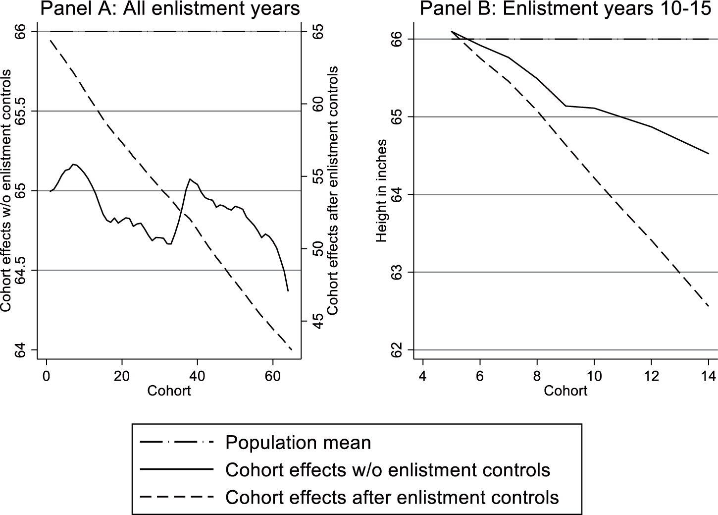
Figure 2 uses these simulated data to illustrate the fundamental econometric problem of the approach Komlos and A’Hearn claim corrects for selection bias. Figure 2A reports results for all individuals in cohorts born over 70 years. The solid line reports cohort trends in height, adjusted using a regression model that has dummies for birth-year alone. (The results in this case are of course identical to what one would obtain by computing the mean height in the selected sample for each birth cohort.) The mean height for the selected sample usually lies below the population mean of 66 inches, and the bias differs by cohort. The dashed lined in Figure 2A reflects the cohort trend estimated as Komlos and A’Hearn recommend, adding enlistment-year dummies to the model with birth-cohort dummies. Note that the vertical axes in Figure 2A are different:their proposed correction for sample-selection bias makes the problem significantly worse. This approach implies that cohort specific heights fell by more than 20 inches over these 70 cohorts, after adjusting for year of enlistment.

Figure 2

BIRTH COHORT EFFECTS IN A SIMULATED MILITARY SAMPLE SUBJECT TO SELECTION

Notes: The vertical axes differ between Panel A and B, and that the two vertical axes in Panel A differ. Every cohort of the simulated population has a mean height of 66 inches (the standard deviation is 2.5 inches). Cohort effects without enlistment controls are estimated using an OLS model with dummies for each birth cohort. Cohort effects after enlistment controls (as recommended by Komlos and A’Hearn) are estimated by adding year-of-enlistment dummies to the model with birth-cohort dummies. The civilian wage grows each year by g_t - g_t-1 where g_t is the Broadberry et al. (Reference Broadberry, Bruce, Klein, Overton and van Leeuwen2015) estimate of British GDP per capita.

Sources: See the text and Bodenhorn, Guinnane, and Mroz (Reference Bodenhorn, Timothy and Thomas2019a, Reference Bodenhorn, Timothy, Thomas, Wolcott and Hanes2019b) and the appendix to that paper for a full explanation of the simulation underlying these figures, as well as the calibration of the Roy model at the heart of that simulation.

The procedure Komlos and A’Hearn recommend does not recover the true, zero change in population height across cohorts. At each point in time, the individuals from the less recent cohorts remaining at risk of first enlistment are a considerably more selected group than those from the more recent cohorts who have had fewer opportunities to enlist. As a consequence, the period-specific wage shocks impact the five at-risk cohorts differentially at the same point in time, with these differentials depending on the history of the prior wage shocks. If the cohort experienced a series of bad civilian wage shocks in the first years it was eligible to join the military, the remaining civilians will consist of only the tallest individuals. Imposing enlistment-year specific effects, constant across the five birth cohorts, implies a model that cannot fit the data. In this instance the econometric model compensates for that specification error by introducing an upward trend in enlistment year “effects” with a steeply declining trend in the birth cohort “effects.” Failing to account appropriately for selection by age can yield large, potentially implausible estimates.

Figure 2B focuses on a subset of this simulated population more nearly akin to the Union Army. We examine only individuals who enlisted in years 10-15 of the simulation (i.e., it includes information for those in cohorts 5-14 who enlisted during years 10 through 15). This approximates the outbreak of a war such as the U.S. Civil War. Once again, the true mean is a constant 66 inches. The solid line again reports the trend in mean heights implied by a model with cohort dummies alone. The dashed line reflects the implied trend in mean heights estimated as Komlos and A’Hearn propose. Even for this restricted sub-set, this approach does not correct for height-based selection; in fact, the approach Komlos and A’Hearn recommend once again implies a substantial negative trend in mean height, where the population exhibits no such trend. ^{Footnote 1} This exercise demonstrates why selection on unobservables related to the outcome of interest is typically referred to as non-ignorable selection. One cannot adjust for selection on unobservables using information on observables alone.

PATRIOTISM AND SOLDIER’S WAGES

Komlos and A’Hearn also discuss what they see as the effects of changes in soldiers’ wages, and patriotism during the war. More generally, they suggest that our Roy-style model of the decision to join the military does not apply in wartime: this simple version of the Roy model is not

applicable to the military in wartime; it was not conceived for situations in which survival itself was uncertain and non-pecuniary factors—such as patriotism—were decisive” (pp. 1144-45). We understand that the risk of death is higher for soldiers during wartime; we do not see how this obviates placing some structure on the decision to accept that risk.

Consider first the issue of rising military wages. We do not doubt their evidence, but their claim that “There is no mistaking the direction of change: military service became economically more attractive over time rather than less so” (p. 1146) misses the point of the Roy model. The economic agent at the heart of the model compares life as a recruit to life as a civilian, evaluating the economic and noneconomic returns to each. Military wages probably increased, but the booming wartime economy offered increasingly better opportunities to men who chose to remain in the civilian labor force. The question is how changes in the attractiveness of both military and civilian life affected the distribution of heights for those who chose to enlist.

Their discussion of patriotism has a similar limitation. Clearly, the Union kept successfully recruiting soldiers, so in aggregate, the better inducements worked. And for some recruits, perhaps, “Patriotism made up the difference” (p. 1145). But for patriotism to produce an army that is an unbiased sample of the population, patriotism and height would have to be correlated in particular ways. Komlos and A’Hearn concede that the Union Army exhibits height-based selection, so we know the correlation of height and patriotism did not fit this description. Nowhere do they argue or model formally why variations in unobserved patriotism over time would remove selection bias after controlling for year-of-enlistment effects.

The general point is this: to understand selection into the Union Army or any other choice-based sample, the cliometrician needs a systematic understanding of the way choices were made by or for the individuals involved. Noting that military wages rose does not tell us how those increases affected the decision to join and how those decisions differed across the height and age distributions. The waxing and waning of patriotic sentiment cannot be doubted, but understanding how those evolving sentiments affect the distribution of heights for new recruits is another step altogether. The simple Roy model we used to motivate our discussion of selection bias is only a modest first effort for addressing dynamic selection issues. The more dynamic simulations we report in Bodenhorn, Guinnane, and Mroz (Reference Bodenhorn, Timothy, Thomas, Wolcott and Hanes2019b) and Figure 2 highlight how difficult it can be to uncover true relationships between height and birth cohorts in the presence of selection in response to a changing environment over calendar time. The general challenge for Komlos and A’Hearn (as well as for ourselves, and for anyone else working in this area) is to understand the selection process that accounts for inclusion in a choice-based sample. For a volunteer military force, the selection process reflects not only who the army will accept but more importantly who will join and at what age. Our Roy-style model was motivated by our desire to understand the logic of those concurrent decisions.