2.1 Harmonic decomposition for non-parallel boundary layers

We consider a turbulent boundary layer developing on a flat plate with constant free-stream velocity. The mean flow is assumed homogeneous along the span, but develops slowly in the streamwise direction and varies rapidly in the wall-normal direction. As such, the fluctuations $\boldsymbol{q}^{\prime }$ in (2.3) may be Fourier transformed in the homogeneous spanwise direction and in time. Unless a locally parallel flow approximation is made, however, the streamwise development of $\overline{\boldsymbol{u}}$ precludes a decomposition of $\boldsymbol{q}^{\prime }$ into Fourier modes with constant streamwise wavenumber. Following a PSE-like decomposition, a spatially evolving field of constant frequency $\unicode[STIX]{x1D714}$ and spanwise wavenumber $\unicode[STIX]{x1D6FD}$ may be described by

(2.4) $$\begin{eqnarray}\displaystyle & \displaystyle \boldsymbol{q}^{\prime }(\boldsymbol{x},t)=\hat{\boldsymbol{q}}(x,y)\exp [\text{i}\unicode[STIX]{x1D6E9}(x,z,t)], & \displaystyle\end{eqnarray}$$

(2.5) $$\begin{eqnarray}\displaystyle & \displaystyle \unicode[STIX]{x1D6E9}(x,z,t)=\int _{x_{0}}^{x}\unicode[STIX]{x1D6FC}(\unicode[STIX]{x1D709})\,\text{d}\unicode[STIX]{x1D709}+\unicode[STIX]{x1D6FD}z-\unicode[STIX]{x1D714}t, & \displaystyle\end{eqnarray}$$

where the streamwise wavenumber is represented by $\unicode[STIX]{x1D6FC}=\unicode[STIX]{x1D6FC}(x)$ and the spatial coordinates by $x,y,z$ for the streamwise, wall-normal and spanwise directions, respectively. Equation (2.4) then decomposes the fluctuating field into a wave-like component described by the exponential term with corresponding amplitudes $\hat{\boldsymbol{q}}$ . These functions or ‘modes’ are convective, or form travelling waves, with local phase speed $c=\unicode[STIX]{x1D714}/\unicode[STIX]{x1D6FC}$ . Note that because the decomposition (2.4) is the product of two $x$ -dependent functions, an ambiguity arises as both oscillations and energy growth/decay may be absorbed into either the amplitude functions $\hat{\boldsymbol{q}}$ or the exponential term for $\unicode[STIX]{x1D6FC}\in \mathbb{C}$ . In this study, we take $\unicode[STIX]{x1D6FC}$ to be a strictly real parameter such that streamwise oscillations are contained in the exponential and absorb the fluctuation energy into the amplitude functions. An auxiliary constraint is then implemented to determine the streamwise variation of $\unicode[STIX]{x1D6FC}$ . A similar approach has been considered in Tempelmann, Hanifi & Henningson (Reference Tempelmann, Hanifi and Henningson2010) to capture non-modal growth in three-dimensional laminar boundary layers, although the specification of the real streamwise wavenumber was done differently. Details of the method for determining $\unicode[STIX]{x1D6FC}(x)$ , and a comparison with the classical PSE approach, are delayed until § 2.5. The same decomposition may then be considered for the turbulent forcing term, such that $\boldsymbol{f}^{\prime }=\hat{\boldsymbol{f}}(x,y)\exp [\text{i}\unicode[STIX]{x1D6E9}(x,z,t)]$ .

Substitution of (2.4) into (2.3) yields an equation governing the global spatial distribution of the amplitude functions $\hat{\boldsymbol{q}}(x,y)$ . However, as the boundary layer develops slowly in the streamwise direction, this implies both the amplitude functions and streamwise wavenumber $\unicode[STIX]{x1D6FC}$ are also slowly varying in $x$ . Formally, we may introduce a conventional boundary layer scaling to eliminate terms $O(Re^{-2})$ and higher to obtain

(2.6) $$\begin{eqnarray}\displaystyle \frac{\unicode[STIX]{x2202}\hat{u} }{\unicode[STIX]{x2202}x}+\text{i}\unicode[STIX]{x1D6FC}\hat{u} +\frac{\unicode[STIX]{x2202}\hat{v}}{\unicode[STIX]{x2202}y}+\text{i}\unicode[STIX]{x1D6FD}{\hat{w}}=0, & & \displaystyle\end{eqnarray}$$

(2.7) $$\begin{eqnarray}\displaystyle & & \displaystyle -\text{i}\unicode[STIX]{x1D714}\hat{u} +\bar{u}\left(\frac{\unicode[STIX]{x2202}\hat{u} }{\unicode[STIX]{x2202}x}+\text{i}\unicode[STIX]{x1D6FC}\hat{u} \right)+\bar{v}\frac{\unicode[STIX]{x2202}\hat{u} }{\unicode[STIX]{x2202}y}+\hat{u} \frac{\unicode[STIX]{x2202}\bar{u}}{\unicode[STIX]{x2202}x}+\hat{v}\frac{\unicode[STIX]{x2202}\bar{u}}{\unicode[STIX]{x2202}y}\nonumber\\ \displaystyle & & \displaystyle \quad =-\frac{\unicode[STIX]{x2202}\hat{p}}{\unicode[STIX]{x2202}x}-\text{i}\unicode[STIX]{x1D6FC}\hat{p}+\frac{1}{Re}\left(\frac{\unicode[STIX]{x2202}^{2}\hat{u} }{\unicode[STIX]{x2202}y^{2}}-(\unicode[STIX]{x1D6FC}^{2}+\unicode[STIX]{x1D6FD}^{2})\hat{u} \right)+\hat{f}_{u},\end{eqnarray}$$

(2.8) $$\begin{eqnarray}\displaystyle & & \displaystyle -\text{i}\unicode[STIX]{x1D714}\hat{v}+\bar{u}\left(\frac{\unicode[STIX]{x2202}\hat{v}}{\unicode[STIX]{x2202}x}+\text{i}\unicode[STIX]{x1D6FC}\hat{v}\right)+\bar{v}\frac{\unicode[STIX]{x2202}\hat{v}}{\unicode[STIX]{x2202}y}+\hat{u} \frac{\unicode[STIX]{x2202}\bar{v}}{\unicode[STIX]{x2202}x}+\hat{v}\frac{\unicode[STIX]{x2202}\bar{v}}{\unicode[STIX]{x2202}y}\nonumber\\ \displaystyle & & \displaystyle \quad =-\frac{\unicode[STIX]{x2202}\hat{p}}{\unicode[STIX]{x2202}y}+\frac{1}{Re}\left(\frac{\unicode[STIX]{x2202}^{2}\hat{v}}{\unicode[STIX]{x2202}y^{2}}-(\unicode[STIX]{x1D6FC}^{2}+\unicode[STIX]{x1D6FD}^{2})\hat{v}\right)+\hat{f}_{v},\end{eqnarray}$$

(2.9) $$\begin{eqnarray}\displaystyle -\text{i}\unicode[STIX]{x1D714}{\hat{w}}+\bar{u}\left(\frac{\unicode[STIX]{x2202}{\hat{w}}}{\unicode[STIX]{x2202}x}+\text{i}\unicode[STIX]{x1D6FC}{\hat{w}}\right)+\bar{v}\frac{\unicode[STIX]{x2202}{\hat{w}}}{\unicode[STIX]{x2202}y}=-\text{i}\unicode[STIX]{x1D6FD}\hat{p}+\frac{1}{Re}\left(\frac{\unicode[STIX]{x2202}^{2}{\hat{w}}}{\unicode[STIX]{x2202}y^{2}}-(\unicode[STIX]{x1D6FC}^{2}+\unicode[STIX]{x1D6FD}^{2}){\hat{w}}\right)+\hat{f}_{w}, & & \displaystyle\end{eqnarray}$$

where the variables have been non-dimensionalized by a reference length, $\ell _{r}$ , and velocity, $U_{r}$ , scale such that $Re=U_{r}\ell _{r}/\unicode[STIX]{x1D708}$ . These are essentially the three-dimensional PSE, where the neglected terms include all those involving $\unicode[STIX]{x2202}_{xx}(),\text{d}_{x}\unicode[STIX]{x1D6FC}$ and $\unicode[STIX]{x1D6FC}\unicode[STIX]{x2202}_{x}()$ . Writing the above equations in matrix operator form yields

(2.10) $$\begin{eqnarray}\displaystyle \unicode[STIX]{x1D5D4}\hat{\boldsymbol{q}}+\unicode[STIX]{x1D5D5}\frac{\unicode[STIX]{x2202}\hat{\boldsymbol{q}}}{\unicode[STIX]{x2202}x}+\unicode[STIX]{x1D5D6}\frac{\unicode[STIX]{x2202}\hat{\boldsymbol{q}}}{\unicode[STIX]{x2202}y}+\unicode[STIX]{x1D5D7}\frac{\unicode[STIX]{x2202}^{2}\hat{\boldsymbol{q}}}{\unicode[STIX]{x2202}y^{2}}=\unicode[STIX]{x1D5D8}\hat{\boldsymbol{f}}, & & \displaystyle\end{eqnarray}$$

which represents a parabolized system in the streamwise direction amenable to a marching solution. Equations (2.10) are solved subject to an initial condition $\hat{\boldsymbol{q}}(x_{0})=\hat{\boldsymbol{q}}_{0}$ with boundary conditions

(2.11) $$\begin{eqnarray}\displaystyle & \displaystyle y=0:\hat{u} =\hat{v}={\hat{w}}=0, & \displaystyle\end{eqnarray}$$

(2.12) $$\begin{eqnarray}\displaystyle & \displaystyle y\rightarrow \infty :\hat{u} ={\hat{w}}=\hat{p}=0, & \displaystyle\end{eqnarray}$$

and specified forcing $\hat{\boldsymbol{f}}$ . The coefficient matrices in (2.10) are defined in appendix A. We note the amplitude functions for the turbulent forcing $\hat{\boldsymbol{f}}$ arise from the quadratic nonlinearity in (2.3). In general, this internal forcing is unknown as it depends on the fluctuating field and the interaction among wavenumbers. However, for a prescribed wavenumber combination, equation (2.10) describes a linear sub-system of the full Navier–Stokes equations relating the system response $\hat{\boldsymbol{q}}$ to a specific forcing amplitude $\hat{\boldsymbol{f}}$ (McKeon & Sharma Reference McKeon and Sharma2010; McKeon, Sharma & Jacobi Reference McKeon, Sharma and Jacobi2013; Moarref et al. Reference Moarref, Sharma, Tropp and McKeon2013; Beneddine et al. Reference Beneddine, Sipp, Arnault, Dandois and Lesshafft2016).

2.2 Solution of the linear sub-system

Upon replacing the wall-normal derivatives by their discrete counterpart, equation (2.10) may be written in semi-discrete form as the generic state-space equation,

(2.13) $$\begin{eqnarray}\displaystyle \frac{\unicode[STIX]{x2202}\hat{\boldsymbol{q}}}{\unicode[STIX]{x2202}x}={\mathcal{A}}(x)\hat{\boldsymbol{q}}+{\mathcal{B}}(x)\hat{\boldsymbol{f}}, & & \displaystyle\end{eqnarray}$$

where we refer to ${\mathcal{A}}$ as the dynamics matrix and ${\mathcal{B}}$ the forcing matrix. Equation (2.13) represents a linear, non-autonomous and non-homogeneous differential equation for the fluctuation amplitude functions $\hat{\boldsymbol{q}}$ subject to a specified forcing $\hat{\boldsymbol{f}}$ . Initially, we may consider the homogeneous solution to (2.13), which satisfies the unforced equation $\unicode[STIX]{x2202}_{x}\hat{\boldsymbol{q}}={\mathcal{A}}\hat{\boldsymbol{q}}$ . As the system is linear, the homogeneous solution may be written as the linear mapping,

(2.14) $$\begin{eqnarray}\displaystyle \hat{\boldsymbol{q}}(x)=\unicode[STIX]{x1D731}(x,x_{0})\hat{\boldsymbol{q}}(x_{0}), & & \displaystyle\end{eqnarray}$$

where $\unicode[STIX]{x1D731}(x,x_{0})$ is referred to as the state transition, or propagator matrix which maps a given state at $x_{0}$ to the current state at $x$ . The principal focus of the present study is on investigating the dynamics of (2.13) via the state-transition matrix. A review of the properties of $\unicode[STIX]{x1D731}$ , in particular for non-autonomous operators, may be found, e.g. in Farrell & Ioannou (Reference Farrell and Ioannou1996).

For known $\unicode[STIX]{x1D731}$ , the particular solution to the non-homogeneous system (2.13) can then be determined using the method of variation of parameters, such that the complete solution is given by

(2.15) $$\begin{eqnarray}\displaystyle \hat{\boldsymbol{q}}(x)=\unicode[STIX]{x1D731}(x,x_{0})\hat{\boldsymbol{q}}(x_{0})+\int _{x_{0}}^{x}\unicode[STIX]{x1D731}(x,\unicode[STIX]{x1D709}){\mathcal{B}}(\unicode[STIX]{x1D709})\hat{\boldsymbol{f}}(\unicode[STIX]{x1D709})\,\text{d}\unicode[STIX]{x1D709}. & & \displaystyle\end{eqnarray}$$

In this case, $\unicode[STIX]{x1D731}(x,\unicode[STIX]{x1D709})$ (or, $\unicode[STIX]{x1D731}(x,\unicode[STIX]{x1D709}){\mathcal{B}}(\unicode[STIX]{x1D709})$ ) is the propagator which maps an input state (forcing) at $\unicode[STIX]{x1D709}$ to an output at $x$ , and is referred to as the resolvent, Green’s function or impulse response of the system (Luchini & Bottaro Reference Luchini and Bottaro2014). Note that if the dynamics matrix ${\mathcal{A}}$ was spatially invariant (i.e. ${\mathcal{A}}\neq {\mathcal{A}}(x)$ ), as would occur if the mean flow $\overline{\boldsymbol{u}}$ was independent of $x$ , then $\unicode[STIX]{x1D731}(x,\unicode[STIX]{x1D709})$ would be given directly by the matrix exponential $\text{e}^{{\mathcal{A}}(x-\unicode[STIX]{x1D709})}$ . Furthermore, if the streamwise variation in the amplitude function is neglected, the constant wavenumber $\unicode[STIX]{x1D6FC}$ would completely describe the streamwise dependence. As such, equation (2.13) could be directly solved to yield the algebraic mapping $\hat{\boldsymbol{q}}=-{\mathcal{A}}^{-1}{\mathcal{B}}\hat{\boldsymbol{f}}$ . The operator $-{\mathcal{A}}^{-1}{\mathcal{B}}$ is then identical to the resolvent operator for parallel flows McKeon & Sharma (Reference McKeon and Sharma2010) and the current parabolized approach given by (2.15) can be seen as a direct extension to slowly developing mean flows.

2.3 Current focus on the homogeneous solution

The full system is characterized by (2.15), including both the response to the internal forcing $\hat{\boldsymbol{f}}$ and the downstream response to the initial state $\hat{\boldsymbol{q}}(x_{0})$ . It is common in linear stability theory to consider the system initially at rest, such that $\hat{\boldsymbol{q}}_{0}=0$ and examine the long-term state response subject to the harmonic forcing $\hat{\boldsymbol{f}}$ . In (2.15), however, the initial condition is defined in space as opposed to time. Furthermore, it is not our intention to model the boundary layer through laminar and transitional stages: the boundary layer is assumed turbulent originating from a virtual origin $x_{vo}$ . At a given downstream position $x_{0}>x_{vo}$ , the fluctuation amplitude $\hat{\boldsymbol{q}}(x_{0})$ is surely non-zero and the homogeneous solution should not be neglected. It implicitly accounts for the cumulative effect of forcing upstream of $x_{0}$ that is not explicitly modelled in (2.15). Moreover, as the sub-system given specified forcing amplitude is linear, we may analyse each term in (2.15) independently. In this study, we focus on the homogeneous solution and the dynamics of the state-transition matrix $\unicode[STIX]{x1D731}(x,x_{0})$ .

As formulated in § 2.4, a direct connection may then be made between the present analysis and the theory of spatial optimal disturbances (Andersson et al. Reference Andersson, Berggren and Henningsin1999; Luchini Reference Luchini2000). The main differences between these approaches are that here we consider a turbulent mean flow as opposed to a laminar base state; we further consider perturbations with non-zero frequency and streamwise wavenumber as to include propagating modes as opposed to purely stationary modes. A related approach for stationary optimal disturbances in turbulent flows has been considered by Uzun et al. (Reference Uzun, Davis, Alvi and Hussaini2017).

We also note the likely overlap between both terms in (2.15). The boundary layer may be assumed to be convection dominated, such that all disturbances are immediately washed downstream by the mean flow with, on average, no upstream propagation (i.e. $\unicode[STIX]{x1D6FC}>0$ ). The largest downstream response will then be given by a sufficiently upstream ‘forcing’. If the forcing amplitude functions $\hat{\boldsymbol{f}}(\unicode[STIX]{x1D709})$ are restricted to a single streamwise plane $x_{0}$ , then both terms in (2.15) become equivalent. We may expect that only large-scale fluctuations survive over large streamwise distances. As such, the homogeneous solution can then be seen as a filter in which only large-scale structures with upstream sensitivity are retained.

2.4 Optimal disturbance formulation

Given the solution (2.14), we seek to determine the initial amplitude functions which maximize the downstream state response. To measure the size of the fluctuations, we choose the local kinetic energy

(2.16) $$\begin{eqnarray}\displaystyle E(\boldsymbol{u}(x))=\int _{0}^{\infty }(|u|^{2}+|v|^{2}+|w|^{2})\,\text{d}y. & & \displaystyle\end{eqnarray}$$

Note the kinetic energy is chosen as it provides both a physically meaningful measure of the fluctuation and it is consistent with the dimension of the internal forcing $\hat{\boldsymbol{f}}$ , which only operates on the velocity components. We then define $\hat{\boldsymbol{u}}=\unicode[STIX]{x1D5E5}\hat{\boldsymbol{q}}$ , or

(2.17) $$\begin{eqnarray}\displaystyle \left(\begin{array}{@{}c@{}}\hat{u} \\ \hat{v}\\ {\hat{w}}\end{array}\right)=\left(\begin{array}{@{}cccc@{}}1 & 0 & 0 & 0\\ 0 & 1 & 0 & 0\\ 0 & 0 & 1 & 0\end{array}\right)\left(\begin{array}{@{}c@{}}\hat{u} \\ \hat{v}\\ {\hat{w}}\\ \hat{p}\end{array}\right), & & \displaystyle\end{eqnarray}$$

where $\unicode[STIX]{x1D5E5}$ is a restriction operator to eliminate the pressure term from the full state vector. Similarly, the velocity vector may be mapped to the full dimension of the state vector using the prolongation operator $\unicode[STIX]{x1D5E3}\hat{\boldsymbol{u}}$ for $\unicode[STIX]{x1D5E3}=\unicode[STIX]{x1D5E5}^{T}$ . Equation (2.16) then defines the energy norm and associated scalar product as $E(\hat{\boldsymbol{u}})=\Vert \hat{\boldsymbol{u}}\Vert ^{2}=\langle \hat{\boldsymbol{u}},\hat{\boldsymbol{u}}\rangle$ .

Following Beneddine et al. (Reference Beneddine, Sipp, Arnault, Dandois and Lesshafft2016), we define an arbitrary velocity state $\unicode[STIX]{x1D74D}(x_{0})$ , for which the downstream velocity response is given by (2.14) as $\unicode[STIX]{x1D74D}(x)=\unicode[STIX]{x1D5E5}\unicode[STIX]{x1D731}(x,x_{0})\unicode[STIX]{x1D5E3}\unicode[STIX]{x1D74D}(x_{0})\equiv \unicode[STIX]{x1D731}_{\boldsymbol{u}}\unicode[STIX]{x1D74D}(x_{0})$ . The amplification, or gain $G$ , from $\unicode[STIX]{x1D74D}(x_{0})$ to $\unicode[STIX]{x1D74D}(x)$ is then defined as

(2.18) $$\begin{eqnarray}\displaystyle G=\frac{\Vert \unicode[STIX]{x1D74D}(x)\Vert ^{2}}{\Vert \unicode[STIX]{x1D74D}(x_{0})\Vert ^{2}}=\frac{\Vert \unicode[STIX]{x1D731}_{\boldsymbol{u}}\unicode[STIX]{x1D74D}(x_{0})\Vert ^{2}}{\Vert \unicode[STIX]{x1D74D}(x_{0})\Vert ^{2}}=\frac{\langle \unicode[STIX]{x1D731}_{\boldsymbol{u}}\unicode[STIX]{x1D74D}(x_{0}),\unicode[STIX]{x1D731}_{\boldsymbol{u}}\unicode[STIX]{x1D74D}(x_{0})\rangle }{\langle \unicode[STIX]{x1D74D}(x_{0}),\unicode[STIX]{x1D74D}(x_{0})\rangle }=\frac{\langle \unicode[STIX]{x1D731}_{\boldsymbol{u}}^{\dagger }\unicode[STIX]{x1D731}_{\boldsymbol{u}}\unicode[STIX]{x1D74D}(x_{0}),\unicode[STIX]{x1D74D}(x_{0})\rangle }{\langle \unicode[STIX]{x1D74D}(x_{0}),\unicode[STIX]{x1D74D}(x_{0})\rangle } & & \displaystyle\end{eqnarray}$$

for $\unicode[STIX]{x1D731}_{\boldsymbol{u}}^{\dagger }$ the adjoint operator of $\unicode[STIX]{x1D731}_{\boldsymbol{u}}$ . The so-called optimal disturbance that leads to maximum amplification, $G_{max}$ , over all possible $\unicode[STIX]{x1D74D}(x_{0})$ , is identified by the solution of the optimization problem

(2.19) $$\begin{eqnarray}\displaystyle G_{max}(x)=\underset{\unicode[STIX]{x1D74D}(x_{0})}{\max }\frac{\langle \unicode[STIX]{x1D731}_{\boldsymbol{u}}^{\dagger }(x,x_{0})\unicode[STIX]{x1D731}_{\boldsymbol{u}}(x,x_{0})\unicode[STIX]{x1D74D}(x_{0}),\unicode[STIX]{x1D74D}(x_{0})\rangle }{\langle \unicode[STIX]{x1D74D}(x_{0}),\unicode[STIX]{x1D74D}(x_{0})\rangle } & & \displaystyle\end{eqnarray}$$

given by the leading eigenvector of $\unicode[STIX]{x1D731}_{\boldsymbol{u}}^{\dagger }\unicode[STIX]{x1D731}_{\boldsymbol{u}}\unicode[STIX]{x1D74D}_{j}(x_{0})=G_{j}\unicode[STIX]{x1D74D}_{j}(x_{0})$ . In the following, we assume the eigenvectors $\unicode[STIX]{x1D74D}_{j}(x_{0})$ have been normalized such that $\Vert \unicode[STIX]{x1D74D}_{j}(x_{0})\Vert ^{2}=1$ and sorted in descending order, such that $g_{1}^{2}\geqslant g_{2}^{2}\geqslant \cdots \,$ where $g_{j}^{2}\equiv G_{j}$ . The corresponding optimal response, also normalized, can be determined as $g_{1}\unicode[STIX]{x1D74D}_{1}(x)=\unicode[STIX]{x1D731}_{\boldsymbol{u}}\unicode[STIX]{x1D74D}_{1}(x_{0})$ .

The question then arises as to how well the optimal response $\unicode[STIX]{x1D74D}_{1}(x)$ approximates the full system response amplitude functions $\hat{\boldsymbol{u}}(x)$ . Following McKeon & Sharma (Reference McKeon and Sharma2010), Beneddine et al. (Reference Beneddine, Sipp, Arnault, Dandois and Lesshafft2016), we note the operator $\unicode[STIX]{x1D731}_{\boldsymbol{u}}^{\dagger }\unicode[STIX]{x1D731}_{\boldsymbol{u}}$ is Hermitian and, as such, the eigenvectors $\unicode[STIX]{x1D74D}_{j}(x_{0})$ may be chosen as an orthonormal basis for $\hat{\boldsymbol{u}}(x_{0})$ such that

(2.20) $$\begin{eqnarray}\displaystyle \hat{\boldsymbol{u}}(x_{0})=\mathop{\sum }_{j}a_{j}\unicode[STIX]{x1D74D}_{j}(x_{0}),\quad a_{j}=\langle \unicode[STIX]{x1D74D}_{j}(x_{0}),\unicode[STIX]{x1D5E5}\hat{\boldsymbol{q}}(x_{0})\rangle . & & \displaystyle\end{eqnarray}$$

Using the relation $g_{j}\unicode[STIX]{x1D74D}_{j}(x)=\unicode[STIX]{x1D731}_{\boldsymbol{u}}\unicode[STIX]{x1D74D}_{j}(x_{0})$ , the velocity response amplitude functions may be written as

(2.21) $$\begin{eqnarray}\displaystyle \hat{\boldsymbol{u}}(x)=\unicode[STIX]{x1D731}_{\boldsymbol{u}}\hat{\boldsymbol{u}}(x_{0})=\mathop{\sum }_{j}a_{j}g_{j}\unicode[STIX]{x1D74D}_{j}(x). & & \displaystyle\end{eqnarray}$$

Note the $\unicode[STIX]{x1D74D}_{j}(x)$ also form an orthonormal basis for the velocity response, as shown by the singular value decomposition of $\unicode[STIX]{x1D731}_{\boldsymbol{u}}=\sum _{j}\unicode[STIX]{x1D74D}_{j}(x)g_{j}\unicode[STIX]{x1D74D}_{j}^{H}(x_{0})$ . Using (2.21), if $g_{1}\gg g_{2}\geqslant g_{3}\cdots \,$ we may consider the velocity response to be approximated by only the first response mode, the so-called rank 1 approximation:

(2.22) $$\begin{eqnarray}\displaystyle \hat{\boldsymbol{u}}(x)\approx \langle \unicode[STIX]{x1D74D}_{1}(x_{0}),\unicode[STIX]{x1D5E5}\hat{\boldsymbol{q}}(x_{0})\rangle g_{1}\unicode[STIX]{x1D74D}_{1}(x). & & \displaystyle\end{eqnarray}$$

As shown by Beneddine et al. (Reference Beneddine, Sipp, Arnault, Dandois and Lesshafft2016), the approximation holds globally (in an $L_{2}$ sense) provided

(2.23) $$\begin{eqnarray}\displaystyle g_{1}^{2}|\langle \unicode[STIX]{x1D74D}_{1}(x_{0}),\unicode[STIX]{x1D5E5}\hat{\boldsymbol{q}}(x_{0})\rangle |^{2}\gg \mathop{\sum }_{j\geqslant 2}g_{j}^{2}|\langle \unicode[STIX]{x1D74D}_{j}(x_{0}),\unicode[STIX]{x1D5E5}\hat{\boldsymbol{q}}(x_{0})\rangle |^{2}, & & \displaystyle\end{eqnarray}$$

which states that the optimal disturbance, or leading response mode, must capture the dominant portion of the total kinetic energy and the initial state must not be well aligned with any of the sub-optimal modes $\unicode[STIX]{x1D74D}_{j}(x_{0}),j\geqslant 2$ . The first of these conditions is easily verified by examining the computed eigenvalues $g_{j}^{2}$ . The second condition, however, stands as a plausible assumption that can be verified a posteriori with experimental comparison.

As shown in § 4, the leading eigenvalue $g_{1}^{2}$ corresponding to the optimal disturbance generally contains a dominant fraction of the total energy at a particular wavenumber/frequency combination. This result, consistent with previous resolvent-based approaches (McKeon & Sharma Reference McKeon and Sharma2010; Moarref et al. Reference Moarref, Sharma, Tropp and McKeon2013), indicates the linear sub-system is highly selective, or the linearized Navier–Stokes equations about the turbulent mean acts as a strong directional amplifier. In fact, the shape of the input forcing, or initial condition, is largely inconsequential so long as there is some non-zero component in the direction of $\unicode[STIX]{x1D74D}_{1}(x_{0})$ . Virtually any input, e.g. randomized, will tend towards the ‘optimal’ output and a power iteration approach to solving (2.19) converges extremely fast. In what follows, similar to previous gain-based studies, we consider inputs $\unicode[STIX]{x1D74D}(x_{0})$ of unit integrated kinetic energy across all frequencies and wavenumbers and examine purely the inherent amplification of the linear operator. That is, in the rank 1 approximation (2.22), we do not consider the weighting $a_{1}=\langle \unicode[STIX]{x1D74D}_{1}(x_{0}),\unicode[STIX]{x1D5E5}\hat{\boldsymbol{q}}(x_{0})\rangle$ or rather assume $a_{1}=1$ . Of course, this is not the case in practical turbulent flows, in particular across all parameter combinations. As such, we can expect only qualitative agreement in the amplitude shape functions and computed amplification spectrum. Knowledge of the response $\hat{\boldsymbol{u}}$ at one or more locations can be used to improve the approximation (Moarref et al. Reference Moarref, Sharma, Tropp and McKeon2013; Beneddine et al. Reference Beneddine, Sipp, Arnault, Dandois and Lesshafft2016), however this is not considered.

2.5 Method for determining the streamwise wavenumber

We now return to the method for updating the streamwise wavenumber introduced in § 2.1. To enforce a slow variation in $\hat{\boldsymbol{q}}$ of the order of the mean flow, the classical PSE approach imposes an auxiliary equation that enforces the kinetic energy of the shape function be independent of $x$ (Herbert Reference Herbert1997). This auxiliary equation removes the ambiguity associated with (2.4) and provides a method to iteratively compute the local streamwise wavenumber $\unicode[STIX]{x1D6FC}(x)$ . However, this is designed as a natural extension to normal modes analysis, with the initial condition generally specified as a local eigenmode. As such, the classical PSE formulation is appropriate to study the streamwise evolution of a modal disturbance in which the spatial growth is specified by a local exponential growth rate $\unicode[STIX]{x1D6FC}_{i}(x)$ .

In the present approach, we do not seek a conventional modal description of the fluctuation amplitudes such that non-modal growth is also captured. The objective is to determine the initial $\hat{\boldsymbol{q}}(x_{0})$ which maximizes the downstream response rather than choosing a local eigenmode and studying its downstream evolution. The streamwise wavenumber is then specified as a real parameter and chosen such that the kinetic energy (2.16) is maximized. Note that $\unicode[STIX]{x1D6FC}(x)$ is chosen locally as part of the downstream marching procedure such that for each discrete streamwise plane $x_{j}$ , $\unicode[STIX]{x1D6FC}(x_{j})$ is chosen as that which maximizes $\langle \unicode[STIX]{x1D74D}(x_{j}),\unicode[STIX]{x1D74D}(x_{j})\rangle$ . In this manner, this inner optimization procedure for $\unicode[STIX]{x1D6FC}$ may be seen as an auxiliary constraint such that streamwise oscillations are captured in the exponential term of (2.4) and the growth at a particular wavenumber/frequency combination are captured in the amplitude response functions $\unicode[STIX]{x1D74D}(x)$ . As the mean flow varies only slowly with $x$ , and in the absence of strong modal growth, this implies $\unicode[STIX]{x1D6FC}$ , $G$ and hence $\unicode[STIX]{x1D74D}$ also vary slowly with $x$ . As noted by Tempelmann et al. (Reference Tempelmann, Hanifi and Henningson2010), in which spatial growth was also absorbed into the amplitude functions with real $\unicode[STIX]{x1D6FC}$ , this approach is limited to non-modal and moderate exponential growth. Modes exhibiting strong exponential growth may violate the slowly varying approximation used in the parabolization step.

The current iteration procedure for $\unicode[STIX]{x1D6FC}$ naturally enforces $\unicode[STIX]{x1D6FC}\rightarrow 0$ as $\unicode[STIX]{x1D714}\rightarrow 0$ . As such, for stationary modes with $\unicode[STIX]{x1D714}=0$ , the method is equivalent to conventional spatial optimal disturbances (i.e. Andersson et al. (Reference Andersson, Berggren and Henningsin1999)). It also follows that, for propagating modes, the optimal streamwise wavenumber is induced by the mean flow and the $(\unicode[STIX]{x1D714},\unicode[STIX]{x1D6FD})$ pair, rather than treated as an independent parameter in the resolvent analysis of McKeon & Sharma (Reference McKeon and Sharma2010), Moarref et al. (Reference Moarref, Sharma, Tropp and McKeon2013). Details of the numeric implementation are given in the following section.

2.6 Computational approach

In (2.10), the wall-normal direction is discretized using a spectral collocation method based on Chebyshev polynomials. The Chebyshev collocation points, defined on the interval $[-1,1]$ , are mapped to the physical domain $[0,y_{max}]$ using the rational mapping given by Hanifi, Schmid & Henningson (Reference Hanifi, Schmid and Henningson1996), chosen to cluster points near the centre of the logarithmic region in the turbulent mean flow. The streamwise direction is discretized on a uniform grid over the interval $[x_{0},x_{f}]$ and the streamwise derivative in (2.10) approximated with a second-order backwards difference. On the first streamwise plane, a first-order scheme is used. Further details of the wall-normal and streamwise discretization are provided in appendix A.

The kinetic energy norm at each streamwise plane may then be written as $E(\hat{\boldsymbol{u}})=\Vert \hat{\boldsymbol{u}}\Vert ^{2}=\hat{\boldsymbol{u}}^{H}\unicode[STIX]{x1D5E0}\hat{\boldsymbol{u}}$ where $\text{}^{H}$ denotes the conjugate transpose and $\unicode[STIX]{x1D5E0}$ is a diagonal, positive definite matrix that contains the appropriate quadrature weights (Clenshaw–Curtis) and grid metrics. For known state-transition matrix $\unicode[STIX]{x1D731}(x_{f},x_{0})$ , the discrete solution to the optimization problem (2.19) is readily obtained by solving the eigenvalue problem

(2.24) $$\begin{eqnarray}\displaystyle G\unicode[STIX]{x1D74D}(x_{0})=(\unicode[STIX]{x1D5E0}_{x_{0}}^{-1}\unicode[STIX]{x1D731}_{\boldsymbol{u}}^{H}(x_{f},x_{0})\unicode[STIX]{x1D5E0}_{x_{f}}\unicode[STIX]{x1D731}_{\boldsymbol{u}}(x_{f},x_{0}))\unicode[STIX]{x1D74D}(x_{0}), & & \displaystyle\end{eqnarray}$$

where the leading eigenvector is referred to as the optimal disturbance with amplification $G_{max}$ .

As previously discussed, because of the spatial development of the mean flow, the operator ${\mathcal{A}}$ in (2.13) is non-autonomous and a general form of state-transition matrix cannot be expressed by standard functions (e.g. the matrix exponential). The alternative is to either directly compute a numerical approximation to the state-transition matrix, after which $\unicode[STIX]{x1D731}_{\boldsymbol{u}}^{H}$ is readily computed, or to adopt an iterative approach by which the action of $\unicode[STIX]{x1D731}_{\boldsymbol{u}}$ and $\unicode[STIX]{x1D731}_{\boldsymbol{u}}^{H}$ are computed by integration of the forward and adjoint equations. The latter avoids direct computation and storage of the state-transition matrix and is the approach taken, for example, by Andersson et al. (Reference Andersson, Berggren and Henningsin1999) and Luchini (Reference Luchini2000) in computing optimal disturbances in the Blasius boundary layer. A similar approach is followed here, slightly modified to compute the optimal streamwise wavenumber as part of the marching procedure. We also note this adjoint approach is trivially extended to the case where $\hat{\boldsymbol{f}}\neq 0$ . The adjoint equations are given in appendix B, derived by formulating the optimization problem as one of optimal control theory and driving to zero all variations in the corresponding Lagrange functional. The adjoint implementation was verified by comparing to the direct approach, by approximating $\unicode[STIX]{x1D731}_{\boldsymbol{u}}$ , for stationary disturbances and the current code has been verified in Uzun et al. (Reference Uzun, Davis, Alvi and Hussaini2017) with the results of Andersson et al. (Reference Andersson, Berggren and Henningsin1999). It should be mentioned the direct approach is only applicable for stationary disturbances due to the inner optimization for the streamwise wavenumber. It is also verified in § 4 that the retrieved optimal disturbance contains a dominant fraction of the total kinetic energy such that the current rank 1 approximation is valid.

The full optimization procedure utilizing the adjoint approach, including the determination of the local streamwise wavenumber, can be summarized as follows:

1. (i) Specify $\unicode[STIX]{x1D6FD}$ , $\unicode[STIX]{x1D714}$ , the initial plane $x_{0}$ , the final plane $x=x_{f}$ (specified in terms of $Re_{\unicode[STIX]{x1D6FF}^{\ast }}$ ) and an initial guess, $\unicode[STIX]{x1D6FC}_{0}$ . The initial condition $\unicode[STIX]{x1D74D}(x_{0})$ is initialized as a random vector.

2. (ii) Solve the forward equations (2.10) (with $\hat{\boldsymbol{f}}=0$ ):

   1. (1) Solve the discretized system at streamwise plane $x_{j}$

      (2.25) $$\begin{eqnarray}\displaystyle \unicode[STIX]{x1D63C}_{j}\unicode[STIX]{x1D74D}(x_{j})=\unicode[STIX]{x1D63D}_{j}\unicode[STIX]{x1D74D}(x_{j-1})+\unicode[STIX]{x1D63E}_{j}\unicode[STIX]{x1D74D}(x_{j-2}) & & \displaystyle\end{eqnarray}$$
      for the local response $\unicode[STIX]{x1D74D}(x_{j})$ . The matrices $\unicode[STIX]{x1D63C},\unicode[STIX]{x1D63D},\unicode[STIX]{x1D63E}$ depend on the local mean flow, the parameters $\unicode[STIX]{x1D6FD},\unicode[STIX]{x1D714}$ , and the local estimate for $\unicode[STIX]{x1D6FC}(x_{j})$ . Note, on the first marching plane, a first-order version of the discretized system is solved.

   2. (2) Evaluate the auxiliary constraint $G=\langle \unicode[STIX]{x1D74D}(x_{j}),\unicode[STIX]{x1D74D}(x_{j})\rangle =\unicode[STIX]{x1D74D}^{H}(x_{j})\unicode[STIX]{x1D5E0}_{x_{j}}\unicode[STIX]{x1D74D}(x_{j})$ .

   3. (3) Update the estimate of the local streamwise wavenumber $\unicode[STIX]{x1D6FC}(x_{j})$ based on $G$ and $\unicode[STIX]{x2202}G/\unicode[STIX]{x2202}\unicode[STIX]{x1D6FC}$ .

   4. (4) Repeat steps (1)–(3) until convergence of $G$ and/or $\unicode[STIX]{x1D6FC}(x_{j})$ within specified tolerance.

   5. (5) Increment $j$ and repeat until the final plane $x_{f}$ .

3. (iii) Obtain the initial condition to the adjoint equation using $\unicode[STIX]{x1D74D}(x_{f})$ according to (B 10)–(B 12).

4. (iv) Solve the adjoint equations (B 7) from $x_{f}$ to $x_{0}$ .

5. (v) Obtain a new estimate for the initial condition (optimal input disturbance) $\unicode[STIX]{x1D74D}(x_{0})$ using the adjoint state at $x_{0}$ and (B 13)–(B 15).

6. (vi) Repeat steps 2–5 until the relative tolerance in $G(x_{f})$ is below a specified value.

The inner optimization with respect to the local streamwise wavenumber is performed using a quasi-Newton line search algorithm. Depending on Reynolds number, the number of collocation points used in the wall-normal direction ranges from $N_{y}=150$ –300. In the streamwise direction, $N_{x}=100$ points are used. To avoid any low Reynolds number effects in the specification of the mean flow (see § 2.8) the minimum initial plane is taken as $x_{0}=0.1x_{f}$ . In select cases, the location of the input plane is also examined, where $x_{0}$ is varied in 20 logarithmically spaced points ranging from $x_{f}-x_{0}=0.9x_{f}$ to $x_{f}^{+}-x_{0}^{+}=10$ where $\text{}^{+}$ denotes scaling based on inner units. In the results presented below, all variables have been scaled by reference length scales at the final output plane $x_{f}$ , e.g. boundary layer thickness $\unicode[STIX]{x1D6FF}\equiv \unicode[STIX]{x1D6FF}_{f}$ is defined as that $x_{f}$ .

2.7 Comments on the amplification mechanisms

The downstream marching procedure to solve (2.10) involves essentially the inverse of the coefficient matrices (see also appendix A). These matrices include the local mean flow $\overline{\boldsymbol{u}}$ and the parameters $\unicode[STIX]{x1D6FC},\unicode[STIX]{x1D6FD},\unicode[STIX]{x1D714}$ . Of these, only the $\unicode[STIX]{x1D5D4}$ matrix is ‘tuneable’ by the specification of wavenumber/frequency. From a numerical point of view, the gain over a given $\unicode[STIX]{x0394}x$ will become large when the diagonal terms of $\unicode[STIX]{x1D5D4}$ become small. For large $Re$ , the viscous contribution may always be assumed small, though not negligible. Therefore, as with a parallel resolvent analysis, we may anticipate large amplifications for $\unicode[STIX]{x1D6FC}=\unicode[STIX]{x1D714}=0$ , or when the convective term is balanced such that $(\unicode[STIX]{x1D6FC}\overline{u}-\unicode[STIX]{x1D714})\rightarrow 0$ .

The first of these conditions corresponds to the stationary disturbances of streamwise velocity streaks classically identified in optimal disturbance theory. In this case, amplification is determined by the off-diagonal terms, dominantly the spanwise wavenumber $\unicode[STIX]{x1D6FD}$ and the streamwise velocity shear $\unicode[STIX]{x2202}_{y}\overline{u}$ . The physical mechanism by which the corresponding structures amplify is generally attributed to the lift-up effect (Ellingsen & Palm Reference Ellingsen and Palm1975; Landahl Reference Landahl1980) by which three-dimensional disturbances act in regions of high mean shear to induce large streamwise velocities. As noted by Luchini (Reference Luchini2000) in the Blasius boundary layer, these structures are necessarily static. For a purely convective mean flow (i.e. no reverse flow, separation, etc.), global oscillations of stationary disturbances, such as those generated by $\unicode[STIX]{x1D714}\neq 0$ but with $\unicode[STIX]{x1D6FC}=0$ , would tend to disrupt the amplification process by the lift-up effect. In the present context of a turbulent mean flow, these stationary disturbances can help guide passive control strategies, as in Pujals, Depardon & Cossu (Reference Pujals, Depardon and Cossu2010), and hence provide valuable information regarding preferential scaling. In describing turbulent fluctuations, however, these stationary disturbances are somewhat ambiguous as they do not contribute to the fluctuation energy and naturally observed structures are convective. Their relation to real turbulent structures is often accompanied by a secondary instability mechanism describing the breakdown to convective disturbances.

The second condition for large amplification corresponds to so-called critical layer behaviour when the phase velocity of the fluctuation matches that of the local mean, or $\unicode[STIX]{x1D714}/\unicode[STIX]{x1D6FC}=\overline{u}$ such that the diagonal terms of $\unicode[STIX]{x1D5D4}$ are minimized. Note the critical layer behaviour is naturally enforced in an integral sense, as the fluctuation is distributed in the wall-normal direction. This concept is also related to the convective non-normality described by Marquet, Lombardi & Chomaz (Reference Marquet, Lombardi and Chomaz2009). The most amplified fluctuation can be seen as that which is optimally transported by the mean flow. As these structures are naturally convective, we expect them to better represent the natural structures observed in turbulent boundary layers. Furthermore, because of this convective nature, the downstream response will be most sensitive to an upstream condition, such that the spatial development of the mean flow will play a prominent role in the selection of the optimal response. The present formulation is then well equipped to identify these structures.

2.8 Turbulent boundary layer mean flow

The solution of (2.10) requires only the specification of the turbulent boundary layer mean flow profile and its gradients at each streamwise position. In the current study, this is modelled using the self-consistent, composite profile proposed by Monkewitz, Chauhan & Nagib (Reference Monkewitz, Chauhan and Nagib2007) for high Reynolds number, zero-pressure-gradient turbulent boundary layers. The composite profile follows a classical scaling of inner, outer wake and logarithmic overlap layers locally given by

(2.26) $$\begin{eqnarray}\displaystyle \frac{\bar{u}(y)}{u_{\unicode[STIX]{x1D70F}}}=U_{inner}^{+}(y^{+})-U_{log}^{+}(y^{+})+U_{\infty }^{+}(Re_{\unicode[STIX]{x1D6FF}^{\ast }})-W_{outer}^{+}(\unicode[STIX]{x1D702}), & & \displaystyle\end{eqnarray}$$

where $u_{\unicode[STIX]{x1D70F}}=(\unicode[STIX]{x1D70F}_{w}/\unicode[STIX]{x1D70C})^{1/2}$ is the wall friction velocity, $y^{+}=yu_{\unicode[STIX]{x1D70F}}/\unicode[STIX]{x1D708}$ is the viscous wall unit (inner coordinate), $U_{\infty }^{+}$ is the free-stream velocity scaled by $u_{\unicode[STIX]{x1D70F}}$ , $Re_{\unicode[STIX]{x1D6FF}^{\ast }}$ is the Reynolds number based on displacement thickness $\unicode[STIX]{x1D6FF}^{\ast }$ , and $\unicode[STIX]{x1D702}=y/\unicode[STIX]{x1D6E5}$ is the outer coordinate, or the wall-normal coordinate scaled by the Rotta–Clauser length scale $\unicode[STIX]{x1D6E5}=U_{\infty }^{+}\unicode[STIX]{x1D6FF}^{\ast }$ . Note in the description of the mean flow by Monkewitz et al. (Reference Monkewitz, Chauhan and Nagib2007), $\unicode[STIX]{x1D6E5}$ is taken as the outer length scale. Although not strictly constant, the conventional 99 % boundary layer thickness $\unicode[STIX]{x1D6FF}$ is roughly $0.22\unicode[STIX]{x1D6E5}$ . This also defines the friction Reynolds number as $Re_{\unicode[STIX]{x1D70F}}\approx 0.22Re_{\unicode[STIX]{x1D6FF}^{\ast }}$ . In the current study, we typically use the more familiar boundary layer thickness $\unicode[STIX]{x1D6FF}$ as the outer scale to ease comparison with experimental data. The explicit expressions for the terms in (2.26) are provided in Monkewitz et al. (Reference Monkewitz, Chauhan and Nagib2007) and are not repeated here for brevity sake. However, the profiles are shown to fit well to experimental data (e.g. Österlund (Reference Österlund1999)) from the wall to the free stream. Monkewitz et al. (Reference Monkewitz, Chauhan and Nagib2007) also provides explicit expressions for the streamwise development of the boundary layer length scales (e.g. the momentum thickness, $\unicode[STIX]{x1D703}(x)$ ) used to compute the spatially evolving mean flow. Cossu et al. (Reference Cossu, Pujals and Depardon2009) provides additional relations to compute the wall-normal velocity component and corresponding mean flow gradients.

Though not explicit in (2.26), the streamwise coordinate $x$ is defined with respect to the virtual origin such that the boundary layer is assumed to be fully developed with self-similar inner and outer mean velocity profiles, from $x=0$ onward. While this may not represent a physical location in real flows, it provides a sensitive metric of the quality of turbulent boundary layer data in that a given experiment should produce the same virtual origin at various streamwise measurement stations. As such, it represents an equivalent development length insensitive to the genesis of the boundary layer. We also note that the same profile was used in the temporal optimal disturbances of Cossu et al. (Reference Cossu, Pujals and Depardon2009), although under the parallel flow approximation. Sample profiles of the turbulent mean flow at various Reynolds numbers investigated in the current study are shown in figure 1.

Figure 1.

Turbulent boundary layer profiles for various Reynolds number, $Re_{\unicode[STIX]{x1D6FF}^{\ast }}$ , for (a) the mean flow plotted in outer units, (b) the mean flow plotted in inner units, with the linear sublayer and logarithmic layer denoted and (c) the spatial development of the turbulent boundary layer mean flow from $Re_{\unicode[STIX]{x1D6FF}^{\ast }}=2\times 10^{3}$ to $Re_{\unicode[STIX]{x1D6FF}^{\ast }}=2\times 10^{4}$ . The contour levels are 20 evenly spaced increments from $\overline{u}/U_{\infty }=0.1$ to 0.99 (i.e. the upper contour denotes the 99 % thickness). Note in (c) the $x$ and $y$ axes are not scaled equally for visualization purposes. Both $\unicode[STIX]{x1D6E5}$ and $\unicode[STIX]{x1D6FF}$ scaling is shown for comparison.

3.1 Scaling of the optimal spanwise wavenumber

Figure 4.

(a) The optimal output, $\hat{u}$ , corresponding to the peak spanwise wavenumber in figure 2 for increasing Reynolds number. The mean flow is also plotted in grey to illustrate the location of the disturbance at the approximate centre of the logarithmic region. The legend is the same as figure 1(a). (b) The variation in optimal spanwise wavelength, $\unicode[STIX]{x1D706}_{max}^{+}$ , and its wall-normal maximum, $y_{max}^{+}$ , with Reynolds number $Re_{\unicode[STIX]{x1D70F}}$ . The solid lines indicate a best fit to $Re_{\unicode[STIX]{x1D70F}}^{1/2}$ . Note an additional Reynolds number of $Re_{\unicode[STIX]{x1D6FF}^{\ast }}=8\times 10^{4}$ ( $Re_{\unicode[STIX]{x1D70F}}\approx 17\,800$ ) was included to verify the identified scaling.

Aside from the absence of a secondary peak in figure 3, the most substantial result is the apparent lack of outer scaling in the spanwise spectrum as the optimal spanwise wavenumber shifts to higher values for increasing Reynolds number. In terms of outer units, this requires the optimal structures to decrease in spanwise wavelength with respect to the local boundary layer thickness. To examine the scaling of the peak wavenumber, the streamwise component of the optimal disturbance is plotted alongside the mean flow in figure 4(a) for various Reynolds number. Note the disturbance velocity has been scaled to match the mean flow for graphical clarity. The wall-normal location of peak disturbance velocity, denoted as $y_{max}^{+}$ , clearly increases with increasing Reynolds number when scaled in viscous units. Further, these profiles are approximately similar in the scaling $y/y_{max}$ . Interestingly, the increase in the inner-scaled wall-normal position of the optimal disturbance is aligned with the increase in the extent of the logarithmic overlap in the mean flow, with the peak disturbance velocity occurring near the centre of the log layer. This result is consistent with the scaling of VLSMs and superstructures observed experimentally in turbulent boundary layers, where Mathis et al. (Reference Mathis, Hutchins and Marusic2009) showed the outer peak in the premultiplied streamwise energy spectra occurred near the geometric mean of the log region. Assuming fixed lower and upper bound estimates for the log region of $y^{+}>100$ and $y/\unicode[STIX]{x1D6FF}<0.15$ respectively, or $100<y^{+}<0.15Re_{\unicode[STIX]{x1D70F}}$ , the geometric mean increases as $y_{c}^{+}\sim 3.9Re_{\unicode[STIX]{x1D70F}}^{1/2}$ .

In figure 4(b), the variation of the optimal spanwise wavelength, corresponding to maximum amplification in figure 3(b), and wall-normal location of maximum disturbance velocity is plotted as a function of $Re_{\unicode[STIX]{x1D70F}}$ . Both the inner-scaled spanwise wavelength and wall-normal position are well described by a $Re_{\unicode[STIX]{x1D70F}}^{1/2}$ dependence, denoted by the fit lines in figure 4(b). The location of the maximum disturbance velocity lies just above the estimated centre of the log layer at $y_{max}^{+}\approx 5.8Re_{\unicode[STIX]{x1D70F}}^{1/2}$ . The optimal spanwise wavelength, $\unicode[STIX]{x1D706}_{z,max}^{+}$ , similarly increases as ${\sim}27Re_{\unicode[STIX]{x1D70F}}^{1/2}$ , leading to constant aspect ratio disturbances with $\unicode[STIX]{x1D706}_{z}\sim 4.7y$ . As expected, the $Re_{\unicode[STIX]{x1D70F}}^{1/2}$ dependence is strictly observed only for the higher Reynolds number cases. In fact, for the lowest Reynolds number $Re_{\unicode[STIX]{x1D70F}}\approx 446$ , the upper bound of the estimated log region, $y>0.15\unicode[STIX]{x1D6FF}$ , lies below the lower bound of $y^{+}>100$ such that no log layer can be said to exist. As noted by Hutchins & Marusic (Reference Hutchins and Marusic2007b ), the overlap between these two positions occurs for $Re_{\unicode[STIX]{x1D70F}}\gtrsim 667$ such that an appreciable log layer occurs only for significantly higher $Re_{\unicode[STIX]{x1D70F}}$ . This is reflected in the scaling observed in figure 4(b).

Figure 5.

(a) Premultiplied streamwise energy density, defined by (3.1), obtained from the optimal output disturbance along the envelope of maximum energy amplification and (b) the streamwise energy density integrated over all spanwise wavenumber contributions, $E_{uu}(y)/Re_{\unicode[STIX]{x1D70F}}^{2}$ . Only the higher Reynolds number cases are shown, $Re_{\unicode[STIX]{x1D70F}}\approx 2230,4460,8920$ .

3.2 Identification of energetic spanwise structure

To determine the spanwise structure with the largest contribution to the total disturbance energy, we use the streamwise component of the optimal disturbance response to construct a rank 1 approximation to the streamwise energy density as a function of spanwise wavenumber. The premultiplied streamwise energy density for stationary disturbances is then defined as

(3.1) $$\begin{eqnarray}\displaystyle E_{uu}(y;\unicode[STIX]{x1D6FD})=\unicode[STIX]{x1D6FD}(g_{1}(\unicode[STIX]{x1D6FD})|u_{1}(y;\unicode[STIX]{x1D6FD})|)^{2}, & & \displaystyle\end{eqnarray}$$

where $u_{1}$ is the streamwise velocity of the optimal disturbance response normalized to unit integrated kinetic energy and $g_{1}$ is the square root of the mode energy. $E_{uu}$ is plotted in figure 5(a) as a function of $\unicode[STIX]{x1D706}_{z}^{+}$ , where only the higher $Re_{\unicode[STIX]{x1D6FF}^{\ast }}$ cases are shown for clarity. Contrary to the pure amplification spectra in figure 3, figure 5(a) reveals two peaks in the premultiplied streamwise energy density. We refer to these peaks here as the inner and outer peaks, in which the outer peak is associated with the log-layer-scaled structures identified in figure 4. In figure 5(a), however, the dominant contribution to the streamwise energy is from the inner peak. The location of this inner peak is constant in both spanwise wavelength and wall-normal position when scaled in wall units, with the contour levels for all three $Re_{\unicode[STIX]{x1D6FF}^{\ast }}$ nearly indistinguishable. Though a direct comparison with streamwise energy of turbulent fluctuations may not be strictly valid as the disturbances here correspond to stationary structures with zero frequency, the scaling of the inner peak in figure 5(a) is consistent with the near wall streaks observed in wall-bounded turbulence. The maximum is seen to occur for $(\unicode[STIX]{x1D706}_{z}^{+},y^{+})\approx (40,10)$ , in reasonable agreement with the well accepted near wall streaks of $\unicode[STIX]{x1D706}_{z}^{+}\approx 100$ centred at $y^{+}\approx 12{-}15$ .

The secondary, outer peak contributes less to the overall energy and shifts to both higher spanwise wavelengths and wall-normal positions scaled in inner units. It should be mentioned, this outer peak is only distinguishable from the inner peak for moderately high $Re_{\unicode[STIX]{x1D6FF}^{\ast }}$ . Similar to the most amplified disturbances shown in figure 4, the location of the secondary peak in the premultiplied streamwise energy density scales with $Re_{\unicode[STIX]{x1D70F}}^{1/2}$ , shifted to slightly smaller positions with $\unicode[STIX]{x1D706}_{z}^{+}\approx 20Re_{\unicode[STIX]{x1D70F}}^{1/2}$ and $y^{+}\approx 5.5Re_{\unicode[STIX]{x1D70F}}^{1/2}$ . The spanwise wavelength and wall-normal position of both the inner and outer peak agree well with the resolvent analysis of Moarref et al. (Reference Moarref, Sharma, Tropp and McKeon2013) in turbulent channel flow, where the inner peak in the premultiplied streamwise energy density was found to occur at $(\unicode[STIX]{x1D706}_{z}^{+},y^{+})\approx (44,11)$ and the middle peak for $\unicode[STIX]{x1D706}_{z}^{+}\approx 20Re_{\unicode[STIX]{x1D70F}}^{1/2}$ and $y^{+}\approx 5.2{-}5.8Re_{\unicode[STIX]{x1D70F}}^{1/2}$ . Note, however, that the results of Moarref et al. (Reference Moarref, Sharma, Tropp and McKeon2013) were obtained for traveling wave solutions integrated over all streamwise wavelengths and temporal frequencies and also contained a dominant peak corresponding to large-scale outer layer structures scaling with the channel height. Such outer-scaled structures are not observed here for stationary modes but will be discussed in § 4.

Finally, the profile of streamwise energy intensity obtained by integrating over all spanwise wavenumbers in figure 5(a) is shown in figure 5(b). A large peak in the streamwise energy is seen at $y^{+}\approx 10$ with amplitude approximately constant with $Re_{\unicode[STIX]{x1D70F}}^{2}$ . Similar to figure 5(a), an outer peak is seen for larger $y^{+}$ values. The location of this outer peak increases in $y^{+}$ with increasing Reynolds number. The amplitude, however, does not scale with $Re_{\unicode[STIX]{x1D70F}}^{2}$ as the inner peak.

4.1 Most amplified propagating modes

Figure 7.

(a) Amplification of the optimal disturbance as a function of spanwise wavenumber and radian frequency, computed for $Re_{\unicode[STIX]{x1D6FF}^{\ast }}=2\times 10^{4}$ . (b) The corresponding phase speed with isocontours of the amplification in (a) are overlaid for reference.

To examine the dependence of optimal disturbance amplification on spanwise wavenumber and frequency, these parameters are discretized on logarithmically spaced grids and the procedure outlined in figure 6 computed for each combination. Here, only the leading mode considered. The computations are truncated when the amplification $G_{max}<1$ . Results for $Re_{\unicode[STIX]{x1D6FF}^{\ast }}=2\times 10^{4}$ are plotted in figure 7(a). The $\lim _{\unicode[STIX]{x1D714}\rightarrow 0}G_{max}$ naturally corresponds to the stationary disturbances discussed in the previous section and the spanwise spectrum at the smallest frequency plotted in figure 7(a) ( $\unicode[STIX]{x1D714}\unicode[STIX]{x1D6FF}/U_{\infty }=0.002$ ) aligns exactly with the amplification spectrum in figure 2(a) for $x_{0}=0.1x_{f}$ . This amplification is approximately constant, or independent of $\unicode[STIX]{x1D714}$ , for $\unicode[STIX]{x1D714}\unicode[STIX]{x1D6FF}/U_{\infty }\lesssim 0.07$ . However, a further increase in frequency leads to an appreciable increase in $G_{max}$ , such that the global optimum in energy amplification occurs for propagating modes and not the stationary modes discussed in § 3.

In figure 7(a), two distinct peaks in energy amplification are seen in the propagating modes. The first peak (in terms of increasing $\unicode[STIX]{x1D714}$ ) is observed for a slightly smaller spanwise wavenumber than the corresponding stationary modes, with $\unicode[STIX]{x1D6FD}\unicode[STIX]{x1D6FF}\approx 10$ and $\unicode[STIX]{x1D714}\unicode[STIX]{x1D6FF}/U_{\infty }\approx 0.3$ . For reference this corresponds to a spanwise wavelength of $\unicode[STIX]{x1D706}_{z}\approx 0.6\unicode[STIX]{x1D6FF}$ and streamwise wavelength, using the computed $\unicode[STIX]{x1D6FC}$ at the output plane, of $\unicode[STIX]{x1D706}_{x}\approx 13.8\unicode[STIX]{x1D6FF}$ . These values are well aligned with reported structures observed in turbulent boundary layers, in particularly the VLSMs or superstructures identified in instantaneous visualizations. In comparison to the previously discussed steady disturbances, the energy amplification associated with this peak increases by approximately 43 %.

The second peak occurring for higher frequency disturbances is the primary, or global, peak in energy amplification at this particular $Re_{\unicode[STIX]{x1D6FF}^{\ast }}$ with ${\sim}51\,\%$ increase in amplification over the stationary modes. This occurs for $\unicode[STIX]{x1D6FD}\unicode[STIX]{x1D6FF}\approx 2.2$ and $\unicode[STIX]{x1D714}\unicode[STIX]{x1D6FF}/U_{\infty }\approx 1.0$ , or spanwise and streamwise wavelengths of $\unicode[STIX]{x1D706}_{z}\approx 2.8\unicode[STIX]{x1D6FF}$ and $\unicode[STIX]{x1D706}_{x}\approx 5.1\unicode[STIX]{x1D6FF}$ , respectively. Note the spanwise wavelength associated with this primary peak is significantly larger than the secondary peak, although the streamwise wavelength is much shorter. As such, the aspect ratio $\unicode[STIX]{x1D706}_{x}/\unicode[STIX]{x1D706}_{z}$ of these higher frequency disturbances are smaller. The spanwise wavelength leading to maximum amplification is also in good agreement with the spanwise scale of conventional optimal disturbances in Blasius boundary layers ( $\unicode[STIX]{x1D706}_{z}\approx 2.8\unicode[STIX]{x1D6FF}$ ) (Andersson et al. Reference Andersson, Berggren and Henningsin1999), and laminar and turbulent channel flow ( $\unicode[STIX]{x1D706}_{z}\approx 3h$ ) (Reddy & Henningson Reference Reddy and Henningson1993; del Álamo & Jiménez Reference del Álamo and Jiménez2006), although those were obtained for stationary disturbances with either infinite or very long streamwise wavelengths.

At this moderate Reynolds number, both peaks are well separated in spectral space. Furthermore, no similarly scaled disturbances were identified in the stationary results such that the corresponding modes appear unique to propagating disturbances. The physical significance of both peaks are discussed in following sections. For frequencies $\unicode[STIX]{x1D714}\unicode[STIX]{x1D6FF}/U_{\infty }\gtrsim 2.2$ , no parameter combination leads to appreciable amplification for the input plane considered, $x_{0}=0.1x_{f}$ . It should be noted, however, if the input plane is moved closer to the output, smaller-scale structures (i.e. higher $\unicode[STIX]{x1D6FD}$ and $\unicode[STIX]{x1D714}$ ) are amplified such that the upper contours in figure 7(a) would continue diagonally to the right. As seen in the stationary disturbances, these small-scale structures have much lower amplification, but cover a much larger spanwise wavenumber and frequency range, such that their energy contribution is significant.

Each parameter combination in figure 7(a) is associated with a unique streamwise wavenumber extracted at the final output plane. As such, we plot the disturbance phase velocity, $c=\unicode[STIX]{x1D714}/\unicode[STIX]{x1D6FC}$ , in figure 7(b), with isocontours of amplification overlaid for reference. Here, the two identified peaks are seen to have phase velocities of approximately $0.7U_{\infty }$ and $0.8U_{\infty }$ , respectively. Similar to the amplification, the phase velocity is approximately constant for fixed $\unicode[STIX]{x1D6FD}$ with increasing frequency for $\unicode[STIX]{x1D714}\unicode[STIX]{x1D6FF}/U_{\infty }\lesssim 0.07$ . For higher frequency disturbances, there is a general increase in phase velocity with increasing frequency, and similarly with decreasing spanwise wavenumber. In accordance with Taylor’s hypothesis, the disturbances are seen to convect at approximately the local mean evaluated near the disturbance peak streamwise velocity. As $\unicode[STIX]{x1D714}$ increases, the corresponding disturbance mode shapes (for example, see figures 10 and 11) begin to lift off the wall, with their maximum contribution centred in regions of higher mean flow velocity. A similar behaviour has been noted in McKeon & Sharma (Reference McKeon and Sharma2010). For large $\unicode[STIX]{x1D714}$ and relatively low $\unicode[STIX]{x1D6FD}$ , the mode shapes can be said to become detached from the wall such that they have negligible contribution in the near wall region (figure 11 a). These are essentially free-stream modes with their wall-normal maximum occurring either in the wake region of the mean flow, or near the edge of the boundary layer, and denoted with phase velocity $c\gtrsim 0.8$ in figure 7(b). Conversely, modes with small frequency but large spanwise wavelength have support over a large wall-normal extent such that they maintain high convection velocity.

Figure 8.

Amplification of the optimal disturbance, (a) $Re_{\unicode[STIX]{x1D6FF}^{\ast }}=2\times 10^{3}$ , (b) $Re_{\unicode[STIX]{x1D6FF}^{\ast }}=2\times 10^{4}$ , (c) $Re_{\unicode[STIX]{x1D6FF}^{\ast }}=4\times 10^{4}$ . Note the contour levels are scaled by the maximum amplification for each $Re$ and are hence not the same.

To examine the Reynolds number scaling, the amplification spectrum in figure 7(a) is computed for varying Reynolds number. Two additional representative cases ranging from low to moderately high $Re_{\unicode[STIX]{x1D6FF}^{\ast }}$ are shown in figure 8. Note the results of figure 7(a) are reproduced in figure 8(b) for reference. In each case, a peak in amplification is observed for $\unicode[STIX]{x1D714}>0$ . This occurs consistently for a slightly lower spanwise wavenumber than for the corresponding stationary optimal. For the lowest $Re_{\unicode[STIX]{x1D6FF}^{\ast }}$ considered (figure 8 a), only a single peak in amplification can be clearly distinguished at $\unicode[STIX]{x1D6FD}\unicode[STIX]{x1D6FF}\approx 2.2$ . This is a direct consequence of the lack of scale separation in the mean flow. The location of this peak with increasing $Re_{\unicode[STIX]{x1D6FF}^{\ast }}$ is approximately constant in the outer-scaled spanwise wavenumber, with a slight increase in $\unicode[STIX]{x1D714}$ . The peak at lower $\unicode[STIX]{x1D714}$ emerges only for the higher $Re_{\unicode[STIX]{x1D6FF}^{\ast }}$ cases. Additional cases not shown here indicate the two peaks become distinguishable for $Re_{\unicode[STIX]{x1D6FF}^{\ast }}\geqslant 1\times 10^{4}$ . Similar to the stationary disturbances, this peak shifts to higher $\unicode[STIX]{x1D6FD}$ with increasing Reynolds number. For the larger $Re_{\unicode[STIX]{x1D6FF}^{\ast }}$ cases in which an appreciable logarithmic overlap layer can be said to occur, the modes associated with this peak have their principal support within the logarithmic region of the mean flow. The increase in spanwise wavenumber is explained by the same reasoning as for the stationary disturbances. As $Re_{\unicode[STIX]{x1D6FF}^{\ast }}$ increases, the centre of the log region moves closer to the wall in outer-scaled units. For $y\propto \unicode[STIX]{x1D706}_{z}$ , this requires smaller spanwise structures and hence larger spanwise wavenumber. Conversely, the modes associated with the higher $\unicode[STIX]{x1D714}$ peak at constant $\unicode[STIX]{x1D6FD}\unicode[STIX]{x1D6FF}\approx 2.2$ are centred in the wake region of the mean flow with constant scaling in outer units. Based on this scaling, and the relative location of the corresponding mode shapes within the boundary layer, we refer to these identified modes as log and wake modes, respectively.

Interestingly, the relative amplification of the two peaks changes with increasing $Re_{\unicode[STIX]{x1D6FF}^{\ast }}$ . In figure 8(a,b), the higher frequency wake modes achieve the highest overall energy amplification. However, as shown in figure 8(c), for $Re_{\unicode[STIX]{x1D6FF}^{\ast }}\geqslant 4\times 10^{4}$ the lower frequency log modes are most amplified. In both cases the amplification increases with $Re_{\unicode[STIX]{x1D6FF}^{\ast }}$ , although clearly at different rates. The amplification of the outer-scaled peak initially increases before approximately saturating for higher $Re_{\unicode[STIX]{x1D6FF}^{\ast }}$ . For $Re_{\unicode[STIX]{x1D6FF}^{\ast }}\geqslant 1\times 10^{4}$ in which the log peak is distinguishable, the amplification increases approximately as $Re_{\unicode[STIX]{x1D6FF}^{\ast }}^{0.75}$ . As such, the log modes becomes increasingly dominant as Reynolds number increases.

4.2 Identification of large-scale energetic propagating modes

The spectra in figure 8 identify propagating modes which amplify by several orders of magnitude given optimal forcing by means of an initial condition. However, the pure amplification spectrum is poorly suited to identify scales which, on average, contain the dominant portion of total fluctuating energy. This is better visualized by the premultiplied amplification, $\unicode[STIX]{x1D6FD}\unicode[STIX]{x1D714}G_{max}$ , such that equal area corresponds to equal contribution to total integrated kinetic energy on a logarithmic scale. In this case, it is immediately obvious that the stationary modes considered in § 3, and the low frequency modes in figure 8, do not appreciably contribute to total kinetic energy and hence not directly representative of the dominant, energetic motions in turbulent boundary layers. The peaks in figure 8 may, however, be more representative of structures visualized in instantaneous snapshots.

Figure 9.

Premultiplied amplification, $\unicode[STIX]{x1D6FD}\unicode[STIX]{x1D714}G_{max}$ , of the optimal disturbance, (a) $Re_{\unicode[STIX]{x1D6FF}^{\ast }}=2\times 10^{3}$ , (b) $Re_{\unicode[STIX]{x1D6FF}^{\ast }}=2\times 10^{4}$ , (c) $Re_{\unicode[STIX]{x1D6FF}^{\ast }}=4\times 10^{4}$ . In (b), the location of the identified log and wake modes are labelled ‘ $\ell$ ’ and ‘ $w$ ’, respectively.

The premultiplied spectra, for the same cases as figure 8, are shown in figure 9. Aside from the absence of low frequency content (note the lower axis limits in figure 9 are different than in figure 8), the premultiplied spectra show similar features. Again at the lowest $Re_{\unicode[STIX]{x1D6FF}^{\ast }}$ considered, there is insufficient scale separation such that only one elongated peak region is observed. For high $Re_{\unicode[STIX]{x1D6FF}^{\ast }}$ , two regions are identified associated with the log and wake modes. These are respectively labelled as ‘ $\ell$ ’ and ‘ $w$ ’ in figure 9. Note the weighting of the premultiplication shifts the locations of these regions to higher spanwise wavenumbers and frequencies as compared to figure 8. Furthermore, for the higher $Re_{\unicode[STIX]{x1D6FF}^{\ast }}$ the log modes increasingly contain the dominant portion of fluctuation energy content. The scaling of the log and wake modes with increasing Reynolds numbers are discussed in the following section.

Figure 10.

Streamwise component of the optimal disturbance response corresponding to the global peak in premultiplied energy amplification at $Re_{\unicode[STIX]{x1D6FF}^{\ast }}=2\times 10^{4}$ (see figure 9 b). (a) Spatial evolution over the full streamwise domain and (b) plotted with equal axis scaling on a shortened streamwise domain. Here, $\unicode[STIX]{x1D6FD}\unicode[STIX]{x1D6FF}=16.5$ ( $\unicode[STIX]{x1D706}_{z}\approx 0.4\unicode[STIX]{x1D6FF}$ ),  $\unicode[STIX]{x1D714}\unicode[STIX]{x1D6FF}/U_{\infty }=0.76$ ( $\unicode[STIX]{x1D706}_{t}=2\unicode[STIX]{x03C0}/\unicode[STIX]{x1D714}\approx 8.3\unicode[STIX]{x1D6FF}/U_{\infty }$ ). At the output, the induced streamwise wavelength is $\unicode[STIX]{x1D706}_{x}\approx 6.1\unicode[STIX]{x1D6FF}$ with phase velocity $c\approx 0.74U_{\infty }$ .

Figure 11.

Streamwise component of the optimal disturbance response corresponding to the secondary peak in premultiplied energy amplification at $Re_{\unicode[STIX]{x1D6FF}^{\ast }}=2\times 10^{4}$ (see figure 9 b). (a) Spatial evolution over the full streamwise domain and (b) plotted with equal axis scaling on a shortened streamwise domain. Here, $\unicode[STIX]{x1D6FD}\unicode[STIX]{x1D6FF}=3.35$ ( $\unicode[STIX]{x1D706}_{z}\approx 1.8\unicode[STIX]{x1D6FF}$ ),  $\unicode[STIX]{x1D714}\unicode[STIX]{x1D6FF}/U_{\infty }=1.38$ ( $\unicode[STIX]{x1D706}_{t}\approx 4.5\unicode[STIX]{x1D6FF}/U_{\infty }$ ). At the output, the induced streamwise wavelength is $\unicode[STIX]{x1D706}_{x}\approx 3.7\unicode[STIX]{x1D6FF}$ with phase velocity $c\approx 0.82U_{\infty }$ .

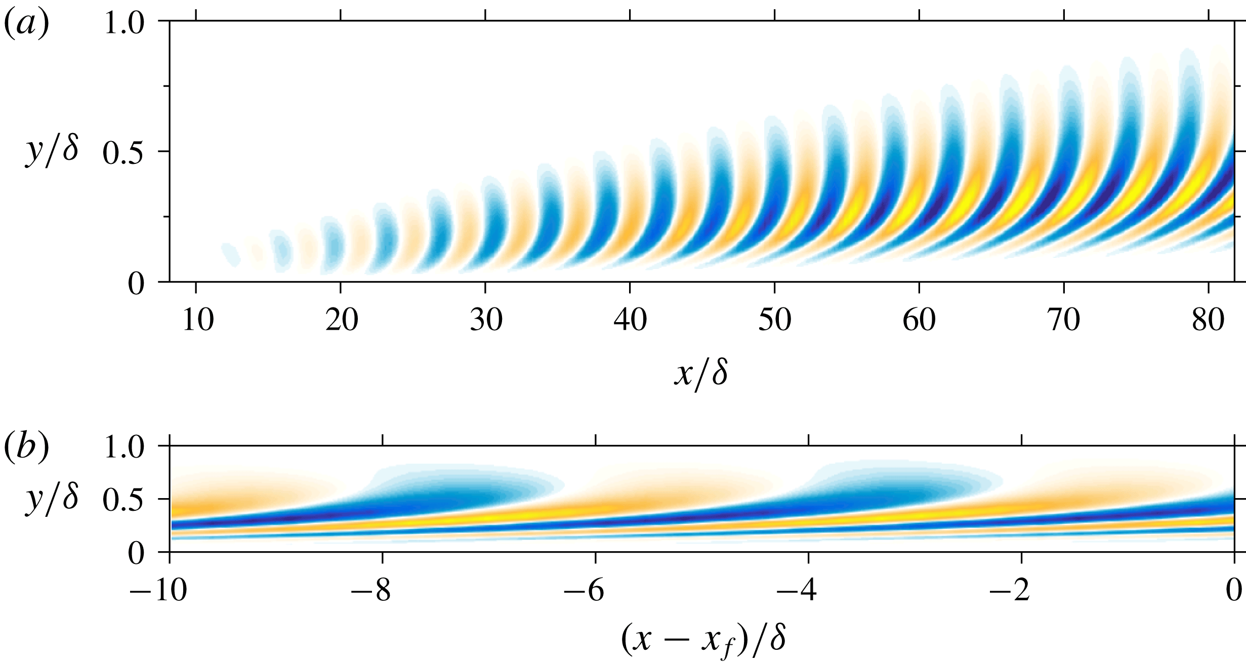
The two classes of structures identified by the peaks in figure 9 are visualized for $Re_{\unicode[STIX]{x1D6FF}^{\ast }}=2\times 10^{4}$ in figures 10 and 11. Note the location of these modes in the premultiplied energy spectrum are those labelled as $\ell$ and $w$ in figure 9(b). The real component of the optimal streamwise velocity response, given by (2.4), is plotted for arbitrary time and spanwise plane. In figure 10(a), the log mode is shown over the entire streamwise domain and again in figure 10(b) for a shortened streamwise domain such that the mode may be visualized with equal axes scaling. The response indicates a wave packet structure attaining its maximum amplitude at the prescribed output plane. As shown in figure 10, the streamwise velocity structures are initially tilted backwards during the early amplification phase and rotate forwards over the streamwise domain as a result of the wall-normal shear. This suggests the Orr mechanism plays a significant role in the early amplification process of these propagating modes, in addition to the optimal alignment of the disturbance phase velocity with that of the local mean. Note the maximum streamwise velocity occurs for $y<0.2\unicode[STIX]{x1D6FF}$ , such that these ‘log modes’ are dominant throughout the log region of the mean flow. Figure 10(b) provides a more realistic picture of the relative streamwise and wall-normal scales, reminiscent of the streamwise velocity streaks reported in turbulent boundary layers. The wavelength corresponds to $\unicode[STIX]{x1D706}_{x}\approx 6.1\unicode[STIX]{x1D6FF}$ , in close agreement with the experimentally observed structures and the outer peak in streamwise velocity spectra (Mathis et al. Reference Mathis, Hutchins and Marusic2009).

Similarly, the streamwise velocity response mode corresponding to the secondary wake mode in figure 9(b) is shown in figure 11. It is immediately recognized that these have a shorter streamwise wavelength than the log modes, with much larger wall-normal extent. They also have significantly less initial upstream tilt, indicating possible reasons why they experience lower amplification than the corresponding log modes (in addition to being centred in a region with less mean shear). As noted in previous discussion, as the wake mode develops in the streamwise direction, it becomes essentially detached from the wall with little to no support in the near wall region. The dominant contribution comes in the wake of the mean flow, well outside the log layer, with the ‘heads’ protruding near the edge of the boundary layer (figure 11 b).

Figure 12.

$Re$ scaling of the most energetic optimal disturbance wavelengths, determined from the peaks in premultiplied energy amplification (see figure 9). (a,c) Peaks corresponding to log-layer modes, (b,d) the peaks corresponding to wake modes. Open symbols represent data from the current model, filled symbols are experimental data estimated from the premultiplied streamwise energy spectra in Mathis et al. (Reference Mathis, Hutchins and Marusic2009) for zero-pressure-gradient turbulent boundary layers. The solid lines represent trend lines. In (c), the dotted line corresponds to $\unicode[STIX]{x1D706}_{x}^{+}=6Re_{\unicode[STIX]{x1D70F}}$ in accordance with the generally accepted scaling of the streamwise wavenumber. In (d) the dotted line corresponds to $\unicode[STIX]{x1D706}_{x}^{+}=3Re_{\unicode[STIX]{x1D70F}}$ .

4.3 Scaling of the propagating modes and comparison with experimental measurements

Here we present the $Re$ -scaling of the most energetic optimal disturbance modes and a comparison to energetic scales observed in turbulent boundary layers. To this end, we extract length scales associated with the log and wake mode peaks in the premultiplied amplification spectra (see figure 9), denoted with the subscript ‘ $\text{max}$ ’, for $Re_{\unicode[STIX]{x1D6FF}^{\ast }}=2\times 10^{3}$ – $1.6\times 10^{5}$ , or $Re_{\unicode[STIX]{x1D70F}}\approx 446$ –36 000. These results are plotted in wall units as a function of $Re_{\unicode[STIX]{x1D70F}}$ in figure 12(a,c) for the log modes and 12(b,d) for the wake modes. We also plot experimental data, estimated from the premultiplied streamwise energy spectra of Mathis et al. (Reference Mathis, Hutchins and Marusic2009) for high $Re$ turbulent boundary layers. In this case, the location of the ‘outer peak’ in the streamwise energy spectra generally associated with ‘superstructures’ (or VLSMs), is plotted alongside the log modes. Similarly, the approximate location of the emergence of the ‘outer hump’, as described by Monty et al. (Reference Monty, Hutchins, Ng, Marusic and Chong2009) and associated with the LSMs, is plotted alongside the wake modes. Note that no matching information is available for the spanwise wavelengths.

Figure 12(a) shows the extracted spanwise and wall-normal scaling the log modes. Similar to the stationary modes in figure 4(b), both the inner-scaled spanwise wavelength and wall-normal position vary approximately as $Re_{\unicode[STIX]{x1D70F}}^{0.5}$ for the $Re$ range considered here. Following the discussion in § 3.1, this $Re_{\unicode[STIX]{x1D70F}}$ -dependence is in agreement with the scaling of the geometric centre of the logarithmic layer of the mean flow, and the approximate location of the peak Reynolds shear stress (Sreenivasan Reference Sreenivasan1989). The wall-normal position of the optimal disturbance energy lies slightly above the location of the outer peak in the experimental measurements. However, the approximate square root scaling is well predicted. The aspect ratio of the log modes remains approximately constant in the streamwise plane, with spanwise wavelength given by $\unicode[STIX]{x1D706}_{z,max}^{+}\approx 26Re_{\unicode[STIX]{x1D70F}}^{1/2}$ . As a practical consideration, note the increase in both $y_{max}^{+}$ and $\unicode[STIX]{x1D706}_{z,max}^{+}$ expressed in wall units is associated with a corresponding decrease in outer units as $Re_{\unicode[STIX]{x1D70F}}^{-1/2}$ (i.e. if $y^{+}\sim Re_{\unicode[STIX]{x1D70F}}^{p}\;\Longrightarrow \;y/\unicode[STIX]{x1D6FF}\sim Re_{\unicode[STIX]{x1D70F}}^{p-1}$ for arbitrary power, $p$ ). This requires the energetic modes move closer to the wall relative to local boundary layer thickness with decreasing spanwise wavelength as $Re$ increases.

The streamwise wavelength of the log mode displays different scaling than the wall-normal and spanwise scales, as shown in figure 12(c). A simple linear regression analysis on the logarithmic-scaled data yields $\unicode[STIX]{x1D706}_{x,max}^{+}\sim Re_{\unicode[STIX]{x1D70F}}^{0.7}$ , indicating a Reynolds number dependence and hence slight shortening in streamwise length relative to the boundary layer thickness. Note the two lower $Re_{\unicode[STIX]{x1D70F}}$ points have not been included in the fit as there is no clear distinction between the log and wake modes (see figure 9 a). It is generally accepted the outer peak in premultiplied streamwise energy spectra is approximately fixed in outer units with $\unicode[STIX]{x1D706}_{x}\approx 6\unicode[STIX]{x1D6FF}$ (Hutchins & Marusic Reference Hutchins and Marusic2007a ). This requires the inner-scaled wavelength increase linearly as $\unicode[STIX]{x1D706}_{x}^{+}\approx 6Re_{\unicode[STIX]{x1D70F}}$ (dotted line in figure 12 c). However, recent high Reynolds number experimental data indicate a $Re_{\unicode[STIX]{x1D70F}}^{0.5}$ dependence on the streamwise wavelength associated with the outer peak (Vallikivi, Ganapathisubramani & Smits Reference Vallikivi, Ganapathisubramani and Smits2015). This is in agreement with the present results in that there may be at least a moderate Reynolds number dependence. Nevertheless, the agreement in figure 12(c) between the computed streamwise wavelengths of the optimal disturbance log modes and the outer peak in the experimental measurements over roughly an order of magnitude in $Re_{\unicode[STIX]{x1D70F}}$ is encouraging. Both the best fit and a $6Re_{\unicode[STIX]{x1D70F}}$ trend line are shown for comparison.

In figure 12(b,d), we show the respective scaling of the wake modes and comparison of the approximated LSMs in Mathis et al. (Reference Mathis, Hutchins and Marusic2009). Again, both the spanwise and wall-normal scales of the optimal disturbance modes scale similarly. However, here they show approximately linear increase with $Re_{\unicode[STIX]{x1D70F}}$ , or constant scaling in terms of boundary layer heights. In this case, $y\approx 0.3\unicode[STIX]{x1D6FF}$ with $\unicode[STIX]{x1D706}_{z}\approx 1.7\unicode[STIX]{x1D6FF}$ . Note, consistent with this outer scaling, these modes are centred in the wake region of the mean flow, with diminishing support extending towards the wall (e.g. figure 11). The associated streamwise wavelength, plotted in figure 12(d), reveals a weak $Re_{\unicode[STIX]{x1D70F}}$ -dependence with $\unicode[STIX]{x1D706}_{x}^{+}\sim Re_{\unicode[STIX]{x1D70F}}^{0.9}$ . Similar to the streamwise scales of the log modes, this indicates a slight shortening of $\unicode[STIX]{x1D706}_{x}/\unicode[STIX]{x1D6FF}$ with increasing Reynolds number. Over the range of $Re_{\unicode[STIX]{x1D70F}}$ considered here, $\unicode[STIX]{x1D706}_{x}\approx 3{-}4\unicode[STIX]{x1D6FF}$ , in good agreement with the location of the outer hump in the streamwise energy spectra (Monty et al. Reference Monty, Hutchins, Ng, Marusic and Chong2009). The dotted line in figure 12(d) denotes $\unicode[STIX]{x1D706}_{x}=3\unicode[STIX]{x1D6FF}$ .

5.1 Comparison of results with related gain-based approaches

The current approach is related to several recent studies on the linear amplification properties of the Navier–Stokes equations about wall-bounded flows. In particular, Cossu et al. (Reference Cossu, Pujals and Depardon2009) has studied temporal optimal disturbances with the same mean flow profile used here along with a parallel flow approximation. An eddy viscosity was also included to model the interaction of incoherent background turbulence with the amplified disturbances. Qualitatively, the optimization results in Cossu et al. (Reference Cossu, Pujals and Depardon2009) are similar to the (steady) disturbances presented here in that streaky structures are amplified with spanwise and wall-normal velocity components generating large streamwise velocity response. Quantitative results are quite different, however. Cossu et al. (Reference Cossu, Pujals and Depardon2009) identified two peaks in the amplification spectrum, one corresponding to very large disturbances ( $\unicode[STIX]{x1D706}_{z}\approx 8\unicode[STIX]{x1D6FF}$ ) centred at the edge of the boundary layer and one inner-scaled peak associated with buffer layer structures with scaling similar to near wall streaks ( $\unicode[STIX]{x1D706}_{z}^{+}\approx 81$ ). Negligible amplification was found for structures within the logarithmic region of the mean flow. As such, aside from the inner layer structures identified here in the streamwise energy density, the most amplified disturbances are orders of magnitude different in spanwise wavelength and wall-normal position with the steady optimal disturbances identified in the current results. A potential reason for such discrepancy is the use of the eddy viscosity in Cossu et al. (Reference Cossu, Pujals and Depardon2009) (see also § 5.3). However, using only the molecular viscosity in the temporal optimal disturbance results does not appear to improve the agreement. Note the temporal optimal disturbances may be regarded as fundamentally different than the current spatial implementation, because those disturbances are neither steady nor time harmonic propagating modes as in the current approach.

Recently, Hack & Moin (Reference Hack and Moin2017) have examined propagating optimal disturbances in spatially developing laminar boundary layers within the PSE framework. In contrast to current approach, Hack & Moin (Reference Hack and Moin2017) do not employ an adjoint-based solver but rather use an expansion based on local, parallel eigenfunctions coupled with their downstream evolution via the PSE linear operator. As such, Hack & Moin (Reference Hack and Moin2017) do not evolve the converged optimal disturbance with a single (spatially evolving) streamwise wavenumber. Rather, each spatially evolving eigenfunction develops according to the streamwise wavenumber selected by the PSE auxiliary equation. In the current method, the conventional PSE auxiliary equation is not used. Although the formulation and base flow differ (laminar versus turbulent), Hack & Moin (Reference Hack and Moin2017) also find the largest energy amplification with three-dimensional disturbances of finite frequency resulting from the interaction of the Orr and lift-up mechanisms.

An approach more closely related to the current formulation is the resolvent analysis of Moarref et al. (Reference Moarref, Sharma, Tropp and McKeon2013), although performed for parallel turbulent channel flow. The resolvent approach identifies both steady and propagating modes and the current method degenerates to the same linear operator if the streamwise derivative of the disturbance is neglected. Moarref et al. (Reference Moarref, Sharma, Tropp and McKeon2013) focused on energetic scales based on the rank 1 model of streamwise energy density. Two classes of large scale structures were identified: an outer and so-called middle peak corresponding essentially to the wake and log modes identified here. The wall-normal and spanwise scales of the middle peak are in good quantitative agreement with the present results. The streamwise wavelengths identified here are shorter (i.e. $\unicode[STIX]{x1D706}_{x}\approx 6\unicode[STIX]{x1D6FF}$ as opposed to $\unicode[STIX]{x1D706}_{x}\approx 12{-}16h$ ). However, these are consistent with differences observed experimentally between internal (channel) and external (boundary layer) flows (Monty et al. Reference Monty, Hutchins, Ng, Marusic and Chong2009). The largest difference is seen with regard to the outer peak, or wake modes. The identified wall-normal and spanwise scales are similar, $y\approx 0.45h$ and $\unicode[STIX]{x1D706}_{z}\approx 2h$ in Moarref et al. (Reference Moarref, Sharma, Tropp and McKeon2013) as compared to $y\approx 0.3\unicode[STIX]{x1D6FF}$ and $\unicode[STIX]{x1D706}_{z}\approx 1.7\unicode[STIX]{x1D6FF}$ here. Again, these are consistent with experimentally observed trends. However, in Moarref et al. (Reference Moarref, Sharma, Tropp and McKeon2013), the streamwise scales of the outer peak increased as $\unicode[STIX]{x1D706}_{x}/h\sim 0.1Re_{\unicode[STIX]{x1D70F}}$ indicating an increase in the outer-scaled wavelength with increasing Reynolds number and structures much larger than observed experimentally. In the current spatial approach, the corresponding structures show a slight decrease in outer-scaled streamwise wavelength with increasing Reynolds number and lengths $\unicode[STIX]{x1D706}_{x}\approx 3{-}4\unicode[STIX]{x1D6FF}$ , in good agreement with experimental observations (Monty et al. Reference Monty, Hutchins, Ng, Marusic and Chong2009). Furthermore, Moarref et al. (Reference Moarref, Sharma, Tropp and McKeon2013) showed an increase in the relative strength of the outer peak structures with increasing $Re_{\unicode[STIX]{x1D70F}}$ . In contrast, here we find the relative amplification of the wake modes decreases with $Re_{\unicode[STIX]{x1D70F}}$ such that the log modes become increasingly dominant at higher Reynolds numbers. Of course, a comparison is somewhat limited as the mean flows are different. However, it does appear the spatial implementation significantly alters the development of at least the largest energetic scales.

5.2 Spatial formulation and influence of the spatial development of the mean flow

In the current formulation, the spatial development enters through both the streamwise evolution of the mean flow and through the streamwise development/lifetime of the disturbance. The disturbances are purely harmonic in time. However, these disturbances are ‘transient’ in the streamwise direction. A small disturbance generated far upstream will have negligible amplitude sufficiently far downstream, regardless of the initial amplification.

In comparing with related analyses under parallel approximations, we may then ask which effect is more critical in determining optimal scales: the evolution of the mean flow, or the transient streamwise development of the disturbance. The latter includes any history effects as well. Of course, perhaps for all but the smallest-scale disturbances, these two effects may be inextricably bound. Nevertheless, the identified scaling in §§ 3 and 4 indicates that the disturbance lifetime and local mean flow are the dominant factors in selecting the preferential scales. In all the results presented in this study, although the disturbance evolves in a spatially varying mean flow, the scaling is presented based on the mean flow scales at the final output plane (i.e. the $Re_{\unicode[STIX]{x1D6FF}^{\ast }}$ the case has been labelled). This is consistent with typical experimental measurements. Although we observe some scatter in the $Re$ scaling (e.g. figure 12), which may be expected in particular because the composite mean profile is not self-similar, the identified trends appear to scale quite well using only the mean flow scales at the output. This suggests the optimal scales adjust rather quickly to the local mean flow, despite the fact that the mean flow may be substantially different far upstream where the disturbance was generated (for large scales).

5.3 Turbulent mean flow and eddy viscosity

The nonlinear source term involving the fluctuating Reynolds stresses is treated here as a generic internal forcing at particular wavenumber/frequency combinations (McKeon & Sharma Reference McKeon and Sharma2010; Beneddine et al. Reference Beneddine, Sipp, Arnault, Dandois and Lesshafft2016). This provides a consistent means to study the linear amplification properties of disturbances about a turbulent mean. Note, however, that no explicit distinction is made between the nature of fluctuations in the Reynolds decomposition. Coherent disturbances are rather implied through maximizing kinetic energy and the rank 1 approximation. Alternatively, one may consider a triple decomposition (Reynolds & Hussain Reference Reynolds and Hussain1972) in which the flow is decomposed into a mean, coherent fluctuation, and so-called background turbulent motion. Deriving the equations for the coherent fluctuations generates Reynolds stresses associated with the fluctuations and background turbulence. Modelling the Reynolds stresses of the background turbulence typically involves introducing an eddy viscosity based on the turbulent mean flow (e.g. Viola et al. Reference Viola, Iungo, Camarri, Port-Agel and Gallaire2014). Neglecting them is generally referred to as a quasi-laminar approach, equivalent to assuming the background turbulence only effects the development of the coherent motion implicitly through modification of the turbulent mean flow, with the resulting linearized equations equivalent to those used in the current study.

Figure 13.

Spatial envelope of maximum energy amplification for steady, streamwise elongated disturbances $(\unicode[STIX]{x1D6FC}=\unicode[STIX]{x1D714}=0)$ , computed for $Re_{\unicode[STIX]{x1D6FF}^{\ast }}=2\times 10^{4}$ . (——): quasi-laminar, (– - – - –): eddy viscosity.

In general, use of an eddy viscosity produces larger structures with significantly less amplification, as previously noted. In figure 13, we briefly compare the results of the current spatial approach with those computed using an eddy viscosity as in Cossu et al. (Reference Cossu, Pujals and Depardon2009) for steady disturbances $(\unicode[STIX]{x1D714}=0)$ at $Re_{\unicode[STIX]{x1D6FF}^{\ast }}=2\times 10^{4}$ . We refer to the results without the eddy viscosity as quasi-laminar and note these are identical to the results in § 3. Figure 13 shows the disturbances computed using the eddy viscosity have significantly less amplification ( ${\sim}2$ orders of magnitude) as a result of the additional large artificial dissipation. Furthermore, the eddy viscosity results reveal the two-peak structure, similar to that identified in del Álamo & Jiménez (Reference del Álamo and Jiménez2006) and Cossu et al. (Reference Cossu, Pujals and Depardon2009), with a relatively high amplitude outer peak at small $\unicode[STIX]{x1D6FD}$ and a low amplitude inner peak at high $\unicode[STIX]{x1D6FD}$ . Repeating the calculations at various $Re$ identifies the outer peak with constant scaling in outer units ( $\unicode[STIX]{x1D706}_{z}\approx 3.4\unicode[STIX]{x1D6FF}$ ) and inner peak with constant scaling in wall units ( $\unicode[STIX]{x1D706}_{z}^{+}\approx 80$ ). The inner peak agrees well with the inner peak identified by Cossu et al. (Reference Cossu, Pujals and Depardon2009), with nearly identical amplification. The outer peak, however, occurs for much shorter spanwise wavelength (but with similar amplification), $\unicode[STIX]{x1D706}_{z}\approx 3.4\unicode[STIX]{x1D6FF}$ as compared to $\unicode[STIX]{x1D706}_{z}\approx 8\unicode[STIX]{x1D6FF}$ in Cossu et al. (Reference Cossu, Pujals and Depardon2009). More importantly, the region between the two peaks in the eddy viscosity results has essentially negligible amplification. Note that this local minimum corresponds to the region for which the quasi-laminar results have maximum amplification. This range of spanwise wavelengths has been associated with structures having peak velocity in the log region of the mean flow (§ 3), known to be dominated by energetic motions in real turbulent boundary layers. The minimum amplification in the eddy viscosity results arise because the Reynolds shear stress peaks near the centre of the log layer and as such, the eddy viscosity is high. This tends to dampen the growth of optimal disturbances. We cannot expect the eddy viscosity results to predict the energetic log modes in this gain-based approach, without resorting to a secondary instability mechanism (e.g. Alizard (Reference Alizard2015)). Indeed, attempting to reconstruct streamwise energy density using the eddy viscosity optimal disturbance modes and amplification, as in (3.1) and shown figure 5 for the quasi-laminar results, yields non-physical results.

5.4 Outlook

The current study is focused on the downstream response to upstream initial conditions/forcing (at a single plane), as in conventional spatial optimal disturbances. This has been formulated as the homogeneous solution to the governing equations subject to a distributed, internal turbulent forcing. While the linearized operator examined here includes all the relevant dynamics, it would be beneficial to examine the full solution and optimal response to distributed forcing. For the boundary layer, the largest scales are most sensitive to upstream forcing. As such, the distributed forcing is likely to have the largest impact on the smallest scales, in which the streamwise location of the forcing amplitude is freely permitted to shift downstream closer to the output optimization plane. In this case, it would be unnecessary to vary the location of the input plane as in § 3 provided the full streamwise domain is sufficiently resolved.

Finally, we have shown that the most energetic optimal disturbances, arising from simple, linear analysis, shows good agreement with energetic motions naturally observed in turbulent boundary layers. In particular, this is especially the case for propagating modes considered with scales resembling LSMs and VLSMs. This supports the view that these structures may be essential, fundamental elements to wall turbulence (Sharma & McKeon Reference Sharma and McKeon2013). Of course, real turbulent motions are not optimized or linear. As the amplification presented here is computed as the response to unit forcing across all frequencies and wavenumbers, quantitative differences may be expected between the predicted optimal scales and the structures observed in natural turbulent boundary layers. This analysis examines the optimized response to forcing, but makes no attempt at describing how or if a particular forcing may occur in real turbulent flows. However, we would expect a large response if the boundary layer is artificially forced at the most amplified wavenumbers/frequencies. As such, the present results may also serve to guide potential passive and active control schemes, in particular when a finite streamwise domain is considered.