1. Introduction
The traditional patrol inspection work [Reference Wu, Sun, Han, Chen, Liu and Wu1] is completed manually, which will not only consume a lot of human and material resources but also will result in certain dangers for patrol inspectors and concerns about inadequate inspection in dangerous environments and special weather. Therefore, the birth of intelligent inspection robot has well solved the problems of large investment of manpower, high cost, low efficiency, unreliability and certain dangers in inspection work. The operation of the inspection robot [Reference Gao, Li, Wang and Chen2–Reference Liang, Cai, Zhao, Chang, Wang and Lv4] is only related to the power and its own quality and will not be affected by dangerous environment and special weather. In addition, the flexibility of the inspection robot is not limited by time and place. Therefore, compared with manual inspection, it will greatly reduce the cost and improve the efficiency and reliability of the inspection process, when the important, complex and repeated inspection tasks are handed over to the inspection robots. The inspection robot working in a specific environment needs to design and plan its path according to the actual conditions. Path planning [Reference Hichri, Gallala, Giovannini and Kedziora5, Reference Ras, Drr and Pr6] means that the inspection robot searches an optimal or suboptimal path from the starting point to the target point according to some specific constraints, such as meeting the requirements of the shortest time, the shortest distance and the least energy, so as to achieve the purposes of high efficiency, high precision and low consumption. In order to achieve these purposes, the path planning research of the inspection robot is generally divided into three steps: (1) Environment modelling; (2) Planning a path that meets the requirements using the optimization algorithm; (3) Processing the planned path (such as smoothing the path to reduce the number of turns).
The path planning of inspection robot is mainly the selection of intelligent optimization algorithm [Reference Tang and Ma7, Reference Deng, Chen, Liu, Zhang and Zhao8]. An excellent optimization algorithm plays a vital role in the path planning of inspection robot. In recent years, bionic intelligent optimization algorithm has become a hot spot to solve various optimization problems. The popular algorithms include Genetic Algorithm (GA), Particle Swarm Optimization (PSO), Ant Colony Optimization (ACO), Artificial Bee Colony optimizer (ABC), Cuckoo Search algorithm (CS), Grey Wolf Optimizer (GWO), and Whale Optimization Algorithm (WOA). Although various optimization algorithms have made great achievements in the application of path planning, there are still some problems in the operation process, such as falling into local optimization, poor stability, slow convergence speed and poor selection accuracy. Because of these limitations, many scholars have made further research and improvement. Xiaohai Wang et al. introduced the restricted mutation generation area into the GA, which increased the search ability of the algorithm near the optimal path in the later stage, shortened the planning time and improved the feasibility of the algorithm [Reference Wang and Meng9]. A. Arikere et al. used multi-objective genetic algorithm to search the optimal solution of the double wishbone design problem [Reference Arikere, Kumar and Bandyopadhyay10]. Yubing Wang et al. proposed a distributed PSO algorithm for fast convergence, random cross-search and accurate search to avoid falling into local optimization and improve algorithm performance [Reference Wang, Bai, Liang, Wang, Zhang and Fu11]. Yuesheng Tan et al. used PSO to train the initial parameters of the ACO, so that the ACO has higher solution quality and faster convergence speed [Reference Tan, Ouyang, Zhang, Lao and Wen12]. C. Pozna et al. proposed a hybrid meta-heuristic optimization algorithm that combines particle filter and particle swarm optimization (PSO) algorithms and applied it to the optimal tuning of PI fuzzy controller [Reference Pozna, Precup, Horvath and Petriu13]. Priyanka sudhakara et al. optimized the fitness function and initialization strategy of the ABC optimization algorithm, improving the performance of the algorithm [Reference Sudhakara, Ganapathy and Sundaran14]. Wenjie Wang et al. set the size of the step size control factor in the CS algorithm as a variable varying with the number of iterations, which accelerated the convergence speed of the algorithm and prevented falling into the local optimal solution prematurely [Reference Wang, Tao, Cao, Wang and Zhang15]. Guangqiang Li et al. proposed an algorithm to select the best individuals from the population to create an adaptive elite set and improve its guidance strategy in view of the lack of balance in the exploration and utilization of WOA algorithm in different positions in the search space [Reference Li, Dong, Wang, Zhu and Liu16].
The GWO is a new bionic intelligent algorithm proposed by Mirjalili team in 2014 based on the grey wolf group predation process [Reference Mirjalili, Mirjalili and Lewis17]. The GWO algorithm has the advantages of simple structure, small adjustment parameters and easy realization, and it has the convergence factor that can be adjusted adaptively. It is widely used in robot, UAV, industrial control and other industries. However, the algorithm still has some problems, such as easily falling into local optimization, slow convergence and poor accuracy. Scholars have made many improvements to these problems of GWO algorithm. Zhang Sen et al. used elite reverse learning strategy and simplex method to improve the population diversity, convergence speed and accuracy of the algorithm [Reference Zhang, Luo and Zhou18]. Shijin Li and Fucai Wang used the anti-learning model to solve the problem that the grey wolf algorithm may fall into local optimization and introduced the limit learning machine algorithm model to improve the convergence speed of the improved algorithm [Reference Li and Wang19]. Jingyi Liu et al. integrated the Lion optimization algorithm and dynamic weight into the GWO optimization algorithm to improve the search ability of the algorithm and avoid falling into local optimization [Reference Liu, Wei and Huang20]. Qifang Luo et al. used the method of copy coding to improve the precision, stability and convergence speed of GWO [Reference Luo, Zhang, Li and Zhou21]. AA heidari and P pahlavini combined Lévy flight and greedy selection strategy with the hunting phase of the GWO algorithm to improve population diversity and jump out of local optimization [Reference Heidari and Pahlavani22]. Wei Zhang et al. proposed an adaptive convergence factor adjustment strategy and an adaptive weight factor to improve the convergence accuracy, speed and stability of GWO algorithm [Reference Zhang, Zhang, Wu and Wang23]. Jing Li and Fan Yang used Kent chaos algorithm to initialize the population, enhance the diversity of the population and propose an adaptive control convergence factor to achieve the balance between exploration and mining, and combine it with particle swarm optimization algorithm to accelerate the convergence speed [Reference Li and Yang24]. JS Wang and SX Li proposed an improved GWO based on evolution and elimination mechanism to achieve an appropriate compromise between exploration and development, which can further accelerate the convergence of exploration and development, and improve the optimization accuracy of GWO [Reference Wang and Li25]. M Kohli and S Arora introduced chaos theory into GWO algorithm to accelerate its global convergence speed and improve the performance of the algorithm in engineering problems [Reference Kohli and Arora26]. Teng Zhijun et al. proposed a hybrid GWO based on tent mapping to increase population diversity and improve global search capability [Reference Teng, Lv, Guo and Yuanyuan27]. Mohammad H. Nadimi shahraki et al. improved the GWO algorithm through the hunting search strategy based on dimension learning, enhanced the balance between local search and global search, and maintained diversity [Reference Nadimi-Shahraki, Taghian and Mirjalili28]. M. W. Guo improved the tracking mode and search mode of GWO algorithm to improve the diversity of the population and the balance between exploration and utilization [Reference Guo, Wang, Zhu, Guo and Xie29]. Chengzhi Qu et al. proposed a new grey wolf optimization algorithm based on reinforcement learning, which can control individuals to achieve adaptive switching operation according to cumulative performance [Reference Qu, Gai, Zhong and Zhang30]. Zhang Sen et al. proposed a new meta-heuristic GWO to improve the accuracy, speed and stability of UCAV path planning [Reference Zhang, Zhou, Li and Pan31]. Hui Xu et al. combined the GWO algorithm with the CS algorithm to improve the search mechanism and enhance the global search ability of the GWO [Reference Hui, Xiang and Su32].
This paper proposes a turn point grey wolf optimization (TPGWO) algorithm to solve the defects of GWO algorithm in the application of path planning, such as easily falling into local optimization, slow convergence in the later stage, poor selection accuracy and stability. It is achieved by taking the path planning of inspection robot as the research object, taking the obtained path optimization as the objective function and the environment as the constraint conditions. As shown in Fig. 1, the algorithm is improved from three aspects: population initialization, convergence factor function and fitness function, and the TPGWO algorithm is further applied to the path planning of the inspection robot. It enables the inspection robot to effectively avoid obstacles in different map environments and then select the optimal path better, faster and more stable under the premise of reaching the target point. The optimization performance of the TPGWO algorithm is verified by test functions and simulation experiments.
Improvement of TPGWO in the application of path planning.

2. Establishment of environmental model
2.1. Problem description
In the process of path planning of inspection robot with obstacle avoidance, the environment of inspection robot should be mathematically modelled firstly, and the actual environment should be replaced by a virtual environment. Secondly, the starting point and ending point of inspection robot are given in the environment model, and an intelligent optimization algorithm is used to find a continuous curve from starting point to ending point that meets certain performance indicators and can avoid obstacles, and the curve is considered as the optimal path. This paper improves the GWO algorithm from three aspects: population initialization, convergence factor and fitness function. Combined with the actual working environment of the inspection robot, the simulation experiment is carried out finally. Therefore, before the simulation experiment, it is necessary to establish an appropriate environmental model. The TPGWO algorithm is compared with the GWO algorithm and PSO algorithm, in terms of the length of the path obtained by the three algorithms after path planning, the time consumed on planning and the convergence of the algorithm, so that the TPGWO algorithm is validated.
2.2. Grid map model establishment
Because the grid map [Reference Zhao, Zhan and Liu33, Reference Ren34] is simple, effective and easy to implement, the grid method is used to model the environment of the mobile robot’s running space, and the size and number of grids are determined by comparing the size of obstacles and the size of the robot’s running space. Figure 2 shows the map model used in this paper. The grids in the figure are called grid nodes
 $S$
, such as 2, 3, …, 99,
 $G$
. The white grids represent the area that the robot can pass through, and the black grids represent the location of obstacles in the operating environment, where
 $S$
is the starting point location, and
 $G$
is the target point location. It is assumed that the boundaries of the map and obstacles are established considering the safe distance of the robot, and the robot can be regarded as a particle in the grid map. The robot is in a two-dimensional space, so the height of the robot is ignored, and multiple obstacles are distributed in the environment, and the grid method is used to establish the model. Each obstacle occupies several grids, when there is less than one grid, it is counted as a grid. In this paper, three kinds of grid maps, 10 * 10, 15 * 15 and 20 * 20, are established, respectively, to represent the actual environment with different map areas, and grid maps of each size generate different numbers of obstacles at random.
Path planning grid map model.

3. Grey wolf optimization algorithm
The GWO algorithm is proposed according to the hunting process of grey wolves. Grey wolf hunting is a group behaviour, and the grey wolf group has a very strict hierarchy. The whole grey wolf group is arranged like a pyramid and is divided into four hierarchy systems. As shown in Fig. 3, the leader at the first layer is called
 $\alpha$
wolf; at the second layer is the
 $\beta$
wolf, the direct reports of α wolf;
 $\delta$
wolf is located on the third layer and follows the decision of
 $\alpha$
and
 $\beta$
; on the fourth layer are the lowest level wolves, called the
 $\omega$
wolves.
Grey wolf group rating chart.

The basic idea of the GWO is as follows: after initializing the wolves, select the three wolves with the best fitness as the head wolves and define them as
 $\alpha,\beta$
and
 $\delta$
, and other wolves led by the head wolf, whose positions are updated according to the distance between them and their prey. The prey is then rounded up, and the position of the prey represents the optimal solution. The mathematical model of GWO is mainly established by searching prey, surrounding prey and attacking prey. The mathematical model of grey wolves surrounding its prey is as follows:
 \begin{equation}\vec {D}=|\vec {C}*\vec {X}_{p}(t)-\vec {X}(t)|\end{equation}
 \begin{equation}\vec {X}(t+1)=\vec {X}_{p}(t)-\vec {A}*\vec {D}\end{equation}
Equations (1) and (2), respectively, represent the distance between grey wolf, prey and the position update of grey wolf individuals, where
 $t$
is the current iteration number,
 $\vec {D}$
represents the length vector between grey wolf and prey,
 $\vec {X_{\textrm{p}}}(t)$
represents the position vector of the current prey,
 $\vec {X}(t)$
represents the position vector of the current grey wolf,
 $\vec {X}(t+1)$
represents the updated position vector of grey wolf individuals,
 $\vec {A}$
and
 $\vec {C}$
are coefficients vector, and the calculation formula is as follows:
 \begin{equation}\vec {A}=2\vec {a}*\vec {r}_{1}-\vec {a}\end{equation}
 \begin{equation}\vec {C}=2*\vec {r}_{2}\end{equation}
In Eqs. (3) and (4),
 $\vec {r_{1}}$
and
 $\vec {r_{2}}$
are random numbers between [0,1], and
 $\vec {a}$
is the convergence factor. The calculation formula is as follows:
 \begin{equation}|\vec {a}|=2-\frac{2t}{t_{\max }}\end{equation}
In Eq. (5),
 $t_{\max }$
is the maximum number of iterations, as the number of iterations increases,
 $| \vec {a}|$
decreases linearly from 2 to 0, the range of
 $|\vec {A}|$
also decreases, its range varies within the interval
 $[\!-a, a]$
. When
 $|\vec {A}|$
is within the range, the next position of the grey wolf can be anywhere between its current position and the prey position. As shown in Fig. 4(a), when
 $|\vec {A}|\lt 1$
, wolves attack prey, which indicates the development ability of GWO, but it is easy to fall into local optimization. As shown in Fig. 4(b), when
 $| \vec {A}| \gt 1$
, grey wolves will not attack prey, and the grey wolves are forced to separate from prey to find more suitable prey, which emphasizes the exploration ability of GWO and the optimal solution can be searched globally. In Eq. (4), we can see that
 $|\vec {C}|$
is a random value between [0,2]. Unlike A, C has a nonlinear change, which represents the random weight of the grey wolf’s location on the prey, where
 $|\vec {C}|\gt 1$
means significant influence; otherwise, the influence weight is small. The randomness of C helps GWO avoid falling into local optimization in the optimization process.
Schematic diagram of grey wolf preying on and away from prey. (a) Preying on prey. (b) Keep away from prey.

In the process of predation, the grey wolf gradually approaches and surrounds the prey and finally launches an attack on the prey. With continuous iteration, all initial solutions keep approaching the optimal solution, and finally, the optimal solution is obtained; that is, the optimal solution is the head wolf
 $\alpha$
, the second and third solutions are
 $\beta$
wolf and
 $\delta$
wolf, respectively. The location update of grey wolf individuals in the GWO is shown in Fig. 5, where
 $\vec {a}_{1}$
,
 $\vec {a}_{2}$
and
 $\vec {a}_{3}$
means the convergence factor between grey wolf
 $\omega$
and the head wolves
 $\alpha$
,
 $\beta$
and
 $\delta$
, respectively, and
 $\vec {C}_{1}$
,
 $\vec {C}_{2}$
and
 $\vec {C}_{3}$
are the coefficients vector between them, and
 $\vec {D}_{{\unicode[Arial]{x03B1}} }$
,
 $\vec {D}_{{\unicode[Arial]{x03B2}} }$
and
 $\vec {D}_{{\unicode[Arial]{x03B4}} }$
represent the distance vectors between them.
GWO grey wolf position update graph.

The mathematical model of attacking prey in GWO is as follows:
 \begin{equation}\begin{cases} \vec {D}_{\alpha }=|\vec {C}_{1}*\vec {X}_{\alpha }-\vec {X}|\\ \\[-8pt] \vec {D}_{\beta }=|\vec {C}_{2}*\vec {X}_{\beta }-\vec {X}|\\ \\[-8pt] \vec {D}_{\delta }=|\vec {C}_{3}*\vec {X}_{\delta }-\vec {X}| \end{cases}\end{equation}
In Eq. (6),
 $\vec {X}_{{\unicode[Arial]{x03B1}} }$
,
 $\vec {X}_{{\unicode[Arial]{x03B2}} }$
and
 $\vec {X}_{{\unicode[Arial]{x03B4}} }$
represent the current position vector of
 $\alpha$
,
 $\beta$
and
 $\delta$
, respectively;
 $\vec {X}$
indicates the position vector of grey wolf ω, and the update process is shown in Eqs. (7) and (8).
 \begin{equation}\begin{cases} \vec {X}_{1}=\vec {X}_{\alpha }-\vec {A}_{1}*(\vec {D}_{\alpha })\\ \\[-8pt] \vec {X}_{2}=\vec {X}_{\beta }-\vec {A}_{2}*(\vec {D}_{\beta })\\ \\[-8pt] \vec {X}_{3}=\vec {X}_{\delta }-\vec {A}_{3}*(\vec {D}_{\delta }) \end{cases}\end{equation}
 \begin{equation}\vec {X}(t+1)=\frac{\vec {X}_{1}+\vec {X}_{2}+\vec {X}_{2}}{3}\end{equation}
Equations (7) and (8) show location update of grey wolf
 $\omega$
and the final position of grey wolf
 $\omega$
, respectively, where
 $\vec {X}_{1}$
,
 $\vec {X}_{2}$
,
 $\vec {X}_{3}$
represent the updated position vector between grey wolf
 $\omega$
and the head wolf
 $\alpha$
,
 $\beta$
and
 $\delta$
, respectively;
 $\vec {A}_{1}$
,
 $\vec {A}_{2}$
,
 $\vec {A}_{3}$
refer to coefficients vector between grey wolf
 $\omega$
and the head wolf
 $\alpha$
,
 $\beta$
and
 $\delta$
;
 $\vec {X}(t+1)$
represents the vector sum of
 $\vec {X}_{1}$
,
 $\vec {X}_{2}$
and
 $\vec {X}_{3}$
, the final updated location of grey wolf ω.
The optimization process of GWO algorithm starts from the random initialization of the population. In the iterative process, the position is updated according to the distance between the three wolves with the best fitness
 $\alpha$
,
 $\beta$
and
 $\delta$
and the prey. If the range of the random variable
 $|\vec {A}|\lt 1$
, it determines that the grey wolf is approaching the prey;
 $|\vec {A}|\gt 1$
means that the grey wolf is forced to stay away from the prey to find a more suitable prey, and the best prey will be found in the last iteration. The basic calculation steps of GWO are as follows:
-
1. Initialize the population number N of wolves, the convergence factor
 $\vec {a}$
and the vector coefficients
$\vec {A}$
and
$\vec {C}$
.
-
2. Calculate the fitness of each grey wolf and save the three wolves with the best fitness as
$\alpha$
,
$\beta$
and
$\delta$
. -
3. Update the position of grey wolf and parameters
$\vec {a}$
,
$\vec {A}$
,
$\vec {C}$
according to the formula. -
4. Calculate the individual fitness of grey wolf and update the fitness and position of three head wolves.
-
5. Judge whether the maximum number of iterations has been reached and output the position of the head wolf
$\alpha$
as the optimal solution, otherwise return to step 3 to continue the calculation.


4. TPGWO
4.1. Initialization improvements
The initialization population of the GWO algorithm is randomly generated, which has the disadvantages of small population and easily falling into local optimization. In order to improve the diversity of the initialization population of the GWO, the population initialization of GWO is improved by using the idea of population crossover and roulette. In the application of TPGWO algorithm in path planning of patrol robot, its initialization population represents each path in the algorithm. The better the fitness of grey wolf individual, the better the superiority of the path is. According to the environmental model in Section 2, the initialization population of GWO in path planning application is the path nodes randomly generated in the grid map. Each path is connected by nodes to form a grey wolf individual. Therefore, the numbers of nodes of each path are the same under the same map. As shown in Fig. 6, the initialized population N1 is crossed to obtain population N2 in TPGWO algorithm, and then, the roulette idea is used to calculate the best fitness in populations N1 and N2 as the initial population N for iterative updating, which can not only improve the search range of the initial population but also improve the quality of the initial population.
Schematic diagram of population initialization improvement.

4.2. Improvement of convergence factor
The convergence factor
 $a$
of the GWO algorithm is a linear decreasing function whose value is from 2 to 0. Its updating mechanism is that the convergence factor searches in the range of [Reference Wu, Sun, Han, Chen, Liu and Wu1, Reference Gao, Li, Wang and Chen2] and converges in the range of [1,0]. Therefore, it is easy to fall into local optimization and the convergence speed is slow. Therefore, the arctangent function and logarithmic function are used to improve the decline curve of the convergence factor
 $a$
, so that the search range of the convergence factor in the early stage is wider and the convergence speed in the later stage is faster. On this basis, the ratio of the number of obstacles to the map area is applied to it, and the parameter value in the function model can be adjusted appropriately to change the turning point of the convergence factor to achieve the optimal selection. The convergence factor function model of the TPGWO algorithm is as follows:
 \begin{equation}k=\frac{\left[\tan (\frac{1-8\arctan 10}{8})+10\right]}{(p*T)}\end{equation}
 \begin{equation}a=\begin{cases} -8\arctan (k*t-10)-8\arctan (10)+2 & t\leq p*T\\ \\[-8pt] \log _{p}^{(t/600)}& t\gt p*T \end{cases}\end{equation}
In Equations (9) and (10),
 $k$
is the adjustment parameter,
 $p$
is the base of the logarithmic function,
 $T$
is the maximum number of iterations, and
 $t$
is the current number of iterations. Some examples are as below:
Taking
 $T=600$
as an example, when the logarithmic function is based on 1/2,
 \begin{equation}k=\frac{\left[\tan (\frac{1-8\arctan 10}{8})+10\right]}{300}\end{equation}
 \begin{equation}a=\begin{cases} -8\arctan (k*t-10)-8\arctan (10)+2 & t\leq 300\\ \\[-8pt] \log _{0.5}^{(t/600)} & t\gt 300 \end{cases}\end{equation}
Equation (12) is the improved convergence factor function when the logarithmic function takes 1/2 as the base, and Fig. 7 shows the change curve. When the logarithmic function takes 1/2 as the base, the denominator of the adjustment parameter
 $k$
in Eq. (11) corresponds to 300.
Variation curve of convergence factor of logarithmic function with the base of ½.

Taking
 $T=600$
as an example, when the logarithmic function is based on 1/3,
 \begin{equation}k=\frac{\left[\tan (\frac{1-8\arctan 10}{8})+10\right]}{200}\end{equation}
 \begin{equation}a=\begin{cases} -8\arctan (k*t-10)-8\arctan (10)+2 &t\leq 200\\ \\[-8pt] \log _{1/3}^{(t/600)} & t\gt 200 \end{cases}\end{equation}
Equation (14) is the improved convergence factor function when the logarithmic function takes 1/3 as the base, and Fig. 8 shows the change curve. When the logarithmic function takes 1/3 as the base, the denominator of the adjustment parameter k in Eq. (13) corresponds to 200.
Variation curve of convergence factor of logarithmic function with the base of 1/3.

Taking
 $T=600$
as an example, when the logarithmic function is based on 2/3,
 \begin{equation}k=\frac{\left[\tan (\frac{1-8\arctan 10}{8})+10\right]}{400}\end{equation}
 \begin{equation}a=\begin{cases} -8\arctan (k*t-10)-8\arctan (10)+2 & t\leq 400\\ \\[-7pt] \log _{2/3}^{(t/600)}& t\gt 400 \end{cases}\end{equation}
Equation (16) is the improved convergence factor function when the logarithmic function takes 2/3 as the base, and Fig. 9 shows the change curve. When the logarithmic function takes 2/3 as the base, the denominator of the adjustment parameter k in Eq. (15) corresponds to 400.
Variation curve of convergence factor of logarithmic function with base 2/3.

From the examples above we can see that, in the research of path planning, it is difficult to find the optimal path in the complex environment map with a large number of obstacles, while it is simple to find the optimal path in the simple environment map with a small number of obstacles. Therefore, in the complex environment map with a large number of obstacles, the search range and search time of the optimization algorithm can be appropriately increased to find the optimal path. On the contrary, in a simple environment map with a small number of obstacles, the search range and search time of the optimization algorithm can be appropriately reduced to find the optimal path. Therefore, the ratio of the number of obstacles to the map area can be added to the function model through the above laws. When the number of obstacles is large and complex, the turning point can be delayed, the iteration times during search can be increased, and the iteration times of convergence can be reduced. When the number of obstacles is small and simple, the turning point can be advanced to reduce the number of iterations during search and increase the number of iterations during convergence.
As a variable value, the base
 $p$
of the logarithmic function can only be used as a fine adjustment in the application of the ratio of the number of obstacles to the map area. In the Eqs. (9) and (10), taking the maximum number of iterations of 600 as an example, when the number of obstacles remains unchanged, let
 $p=\frac{1}{2}$
, the turning point remains unchanged, as shown in
 $a_{1}^{\prime}$
in Eq. (18). When the number of obstacles is relatively small, let
 $p\lt \frac{1}{2}$
, turning point moves forward, as shown in
 $a_{2}^{\prime}$
in Eq. (20), and let
 $p$
be
 $280/600$
to reduce the search time of the algorithm and improve the convergence speed. When there are relatively more and complex obstacles, let
 $p\gt \frac{1}{2}$
, turning point moves backwards, as shown in
 $a_{3}^{\prime}$
in Eq. (22), and let
 $p$
be
 $320/600$
to increase the search time of the algorithm, so that to avoid falling into local optimization and improve the accuracy of the selected path. Equation (23) is the convergence factor function
 $a_{4}^{\prime}$
of the GWO algorithm. Figure 10 shows the comparison of the convergence factor function curves
 $a_{1}^{\prime}$
,
 $a_{2}^{\prime}$
,
 $a_{3}^{\prime}$
and
 $a_{4}^{\prime}$
.
 \begin{equation}k_{1}=\frac{\left[\tan (\frac{1-8\arctan 10}{8})+10\right]}{300}\end{equation}
 \begin{equation}a_{1}^{\prime}=\begin{cases} -8\arctan (k_{1}*t-10)-8\arctan (10)+2 & t\leq 300\\ \\[-8pt] \log _{1/2}^{(t/600)}& t\gt 300 \end{cases}\end{equation}
 \begin{equation}k_{2}=\frac{\left[\tan (\frac{1-8\arctan 10}{8})+10\right]}{280}\end{equation}
 \begin{equation}a_{2}^{\prime}=\begin{cases} -8\arctan (k_{2}*t-10)-8\arctan (10)+2 & t\leq 280\\ \\[-8pt] \log _{280/600}^{(t/600)}& t\gt 280 \end{cases}\end{equation}
 \begin{equation}k_{3}=\frac{\left[\mathit{\tan } (\frac{1-8\mathit{\arctan } 10}{8})+10\right]}{320}\end{equation}
 \begin{equation}a_{3}^{\prime}=\begin{cases} -8\arctan (k_{3}*t-10)-8\arctan (10)+2 & t\leq 320\\ \\[-8pt] \log _{320/600}^{(t/600)} & t\gt 320 \end{cases}\end{equation}
 \begin{equation}a_{4}^{\prime}=2-\frac{t}{300}\end{equation}
Variation curves of functions with different convergence factors.

4.3. Improvement of fitness function
In the application of TPGWO in path planning, its fitness function is the sum of the distances between each node of the path calculated by Euclidean distance. At the same time, the turning times and turning angles of the obtained path are added to the fitness function as penalty values to improve the accuracy of the selected path. In the grid map that built,
 $(x, y)$
is the coordinates of the current node;
 $(x_{1},y_{1})$
is the coordinates of the previous node;
 $(x_{2},y_{2})$
is the coordinates of the next node;
 $V$
is the number of turns;
 $\theta$
is the turning angle;
 $r$
and
 $c$
are the number of rows and columns of the map, respectively. The fitness function is as follows:
 \begin{equation}L=L(i)+\textrm{fix}(M)\end{equation}
 \begin{equation}L(i)=\sqrt{\left(y-y_{1}\right)^{2}+\left(x-x_{1}\right)^{2}}\end{equation}
 \begin{align}\begin{array}{c} \tan \theta _{1}=\dfrac{y-y_{1}}{x-x_{1}}\Rightarrow \theta _{1}=\arctan \dfrac{y-y_{1}}{x-x_{1}}\\ \\[-8pt] \tan \theta _{2}=\dfrac{y_{2}-y}{x_{2}-x}\Rightarrow \theta _{2}=\arctan \dfrac{y_{2}-y}{x_{2}-x} \end{array}\end{align}
 \begin{equation}\theta _{i}=|\theta _{2}-\theta _{1}|\end{equation}
In Eq. (24),
 $L(i)$
is the sum of all nodes in the path, and
 $fix()$
is a rounding function to the left. Equation (25) is the calculation expression of
 $L(i)$
. In Eq. (26),
 $\theta _{1}$
and
 $\theta _{2}$
are the tangent angles between the current node and the previous node, and between the current node and the next node, respectively. In Eq. (27),
 $\theta _{i}$
is the angle difference between the two tangent angles, that is, the angle generated by the current turn. In path planning, if the angle of the obtained path changes, the angle difference of the tangent angle between nodes will occur. Therefore, in the calculation of fitness function, when
 $\tan \theta _{1}\neq \tan \theta _{2}$
, it means that there is a turn in the path, and then
 $V=V+1$
. Every turn will generate a turning angle. In order to facilitate the addition of turning times and angles to the fitness function, the turning times and angles are normalized.
Normalization of turning times and turning angles.

The normalization processing method is shown in Fig. 11, where
 $V$
is the number of turns (V = 1, 2, …), θ is the sum of turning angles, and the turning angle generated each time is between 0° and 360°. When the number of turns is 1,
 $\theta /90^{\circ}$
is 0 to 4; when the number of turns is 2,
 $\theta /90^{\circ}$
is 0 to 8; when the number of turns is 3,
 $\theta /90^{\circ}$
is 0 to 12; when the number of turns is
 $n$
,
 $\theta /90^{\circ}$
is 0 to
 $4n$
. The turning times and turning angles are normalized by the radius M of the arc. The indication shown in Fig. 10 is as follows: when
 $0\leq M\lt 1$
,
 $f=0$
; when
 $1\leq M\lt 2$
,
 $f=1$
; when
 $2\leq M\lt 3$
,
 $f=2$
; when
 $3\leq M\lt 4$
,
 $f=3$
; …; when
 $n-1\leq M\lt n$
,
 $f=n-1$
, where
 $M$
is the corresponding arc radius and
 $f$
is the rounding function to the left. Therefore, the penalty values of turning times and turning angles can be determined by calculating the arc radius
 $M$
, and the arc radius can be determined by the horizontal and vertical coordinates in Fig. 11.
 \begin{equation}\theta =\sum _{i=1}^{V}\theta _{i}\end{equation}
 \begin{equation}A=\frac{\sum _{i=1}^{v}\theta _{i}}{90}=\frac{\theta }{90}\end{equation}
 \begin{equation}M=\sqrt{V^{2}+A^{2}}\end{equation}
Equation (28) is the sum of the turning angles. Equation (29) is to calculate the angle degrees, which divide the sum of the turning angles by 90 to obtain the angle judgment value A, which is the vertical coordinate in Fig. 11. Its horizontal coordinate is the turning times V, and then,
 $(V, A)$
is the coordinate value in Fig. 11. Equation (30) is the size M of the arc radius calculated from the coordinate value, and the penalty value
 $\text{fix}(M)$
can be obtained from the arc radius.
4.4. Summary
This section describes the improvement of TPGWO algorithm in path planning. TPGWO algorithm improves the population initialization of GWO algorithm through the idea of population crossover and roulette to improve the population diversity and changes the linear convergence factor function in GWO algorithm to a nonlinear function to improve the early search range and late convergence speed. Finally, the turning times and turning angles are added to the fitness function to improve the accuracy of the path. The algorithm improvement process is shown in Fig. 12.
Improved flow chart of TPGWO algorithm.

5. Simulation results
In the application of TPGWO, each wolf indicates a path from the start point to the destination in the map. Therefore, the best path can be selected using TPGWO theory proposed in the sections above. In order to verify the superiority of TPGWO in the application of path planning, the convergence of TPGWO is analysed firstly. Secondly, test functions are used to analyse the performance of TPGWO, PSO and GWO. Finally, grid maps with different sizes and obstacles are established, and the planning time and size of the paths obtained by the three algorithms under different maps are compared and analysed. At the same time, the convergence factor function is adjusted in TPGWO according to the number of obstacles, and the planning time and length of the path obtained are compared and analysed.
5.1. Convergence analysis
Theorem 1:
When the parameter
 $a$
in the algorithm gradually decreases from 2 to 0 with the increase of iteration times, the GWO algorithm has convergence.
Proof: It can be seen from the updated formula of GWO
 \begin{align} X\left(t+1\right)&=\frac{1}{3}\left[X_{1}\left(t+1\right)+X_{2}\left(t+1\right)+X_{3}\left(t+1\right)\right]\nonumber\\[3pt] \,&=\frac{1}{3}\left[X_{\alpha }-A_{1}*\left| C_{1}*X_{\alpha }-X\left(t\right)\right| +X_{\beta }-A_{2}*\left| C_{2}*X_{\beta }-X\left(t\right)\right| +X_{\delta }-A_{3}*\left| C_{3}*X_{\delta }-X\left(t\right)\right| \right]\nonumber\\[3pt] \,&=\frac{1}{3}\left[X_{\alpha }-\left(2a_{t}r_{11}-a_{t}\right)\left| 2r_{12}X_{\alpha }-X\left(t\right)\right| +X_{\beta }-\left(2a_{t}r_{21}-a_{t}\right)\left| 2r_{22}X_{\beta }-X\left(t\right)\right|\right.\nonumber\\[3pt] &\quad \left.+\,X_{\delta }-\left(2a_{t}r_{31}-a_{t}\right)\left| 2r_{32}X_{\delta }-X\left(t\right)\right| \right] \nonumber\\[3pt] &=\frac{1}{3}(X_{\alpha }+X_{\beta }+X_{\delta })-\frac{1}{3}a_{t}\left[(2r_{11}-1)\left| 2r_{12}X_{\alpha }-X\left(t\right)\right| +(2r_{21}-1)\left| 2r_{22}X_{\beta }-X\left(t\right)\right| \right.\nonumber\\[3pt] &\quad \left.+\,(2r_{31}-1)\left| 2r_{32}X_{\delta }-X(t)\right| \right]\end{align}
In Eq. (31),
 $X(t)$
is the current position of grey wolves,
 $X(t+1)$
is the next position of grey wolves,
 $X_{\alpha },X_{\beta },X_{\sigma }$
is the current iteration values of wolf
 $\alpha,\beta,\delta$
, respectively,
 $a_{t}$
is the value of convergence factor
 $a$
of the current iteration,
 $r_{11},r_{12},r_{21},r_{22},r_{31},r_{32}$
are random values in [0,1].
Let
 \begin{equation}r_{1}=2r_{11}-1,\hspace{0pt}\,r_{2}=2r_{21}-1,\,r_{3}=2r_{31}-1, \,r_{1},r_{2},r_{3}\in [-1,1]\end{equation}
then
 \begin{equation}X(t+1)=\frac{1}{3}(X_{\alpha }+X_{\beta }+X_{\delta })-\frac{1}{3}a_{t}\left[2r_{1}r_{12}X_{\alpha }-\,r_{1}X(t)+2r_{2}r_{22}X_{\beta }-r_{2}X(t)+2r_{3}r_{32}X_{\delta }+r_{3}X(t)\right]\end{equation}
Let
 \begin{equation}\,r_{1}^{\prime}=2r_{1}r_{12},\hspace{0pt}\,r_{2}^{\prime}=2r_{2}r_{22},\,r_{3}^{\prime}=2r_{3}r_{32},\,r_{1}^{\prime},r_{2}^{\prime},r_{3}^{\prime}\in [\!-2,2]\end{equation}
then
 \begin{equation}X(t+1)=\frac{1}{3}(X_{\alpha }+X_{\beta }+X_{\delta })-\frac{1}{3}a_{t}(r_{1}^{\prime}X_{\alpha }+r_{2}^{\prime}X_{\beta }+r_{3}^{\prime}X_{\delta })+\frac{1}{3}a_{t}(r_{1}+r_{2}+r_{3})X(t)\end{equation}
In GWO,
 $a_{t}$
is a linear decreasing function from 2 to 0, that is,
 $\lim _{t\rightarrow t_{\max }} a_{t}=0$
.
Therefore, when
 $X_{\alpha },X_{\beta },X_{\sigma }$
is constant,
 \begin{equation}\lim _{t\rightarrow t_{\max }} X(t+1)=\frac{1}{3}(X_{\alpha }+X_{\beta }+X_{\delta })\end{equation}
 $t_{max}$
is the maximum number of iterations. Proof completed.
Definition 1: The grey wolf state is composed of the grey wolf position vector, remember that the grey wolf position vector is
 $X$
, and
 $Y$
is the feasible region space of the problem,
 $X\in Y$
, and then, the status of grey wolves is recorded as
 $\mu =(X_{1},X_{2},\cdots,X_{n})$
,
 $X_{i}$
indicates the status of the
 $i\textrm{th}$
grey wolf.
It can be obtained from reference [Reference Zhang, Long, Wang and Yang35], the state sequence
 $\{\mu (t)\colon t\gt 0\}$
of grey wolf population in GWO is a finite Markov chain, and when
 $t_{\max }\rightarrow +\infty$
, the grey wolf group state has ergodicity in the finite state space
 $Y$
. Therefore, the corresponding state
 $X_{\alpha },X_{\beta },X_{\sigma }$
of the three leading wolves
 $\alpha,\beta,\delta$
in the algorithm can be guaranteed to be the global optimal state, the suboptimal state and the third optimal state, respectively. According to the above formula, when
 $t_{\max }\rightarrow +\infty$
, the GWO algorithm has global convergence.
To sum up, the GWO algorithm has convergence, and convergence factor
 $\vec {a}$
has a large impact on convergence. Therefore, this paper mainly changes the convergence factor function from linear decline to nonlinear decline on the basis of GWO and retains the update strategy of the grey wolf algorithm, so it improves the convergence speed of the algorithm in the later period and enhances convergence.
5.2 Algorithm test
In order to test the optimization performance of PSO algorithm, GWO algorithm and the proposed TPGWO algorithm, 16 test functions are used to study and compare, through the statistics of the results of different performance of the three algorithms. Their optimization performance is compared and analysed to verify the effectiveness and feasibility of TPGWO algorithm. In the comparative experiment, in order to compare the fairness, the same experimental parameters and initialization mode are used in the three algorithms. The three algorithms use the same initialization method to get the same starting point. The main parameters of the three algorithms are shown in Table I, and the maximum iteration
 $t_{\max }$
is 600. The test function and its dimension, truth value and function range are shown in Table II. In order to prevent the influence of randomness on the results, each algorithm is run 30 times to take the mean value, and the optimal value, mean value and standard deviation of the algorithm are recorded, respectively. The optimal value reflects the quality of the algorithm, and the mean value shows the accuracy that can be achieved under a given number of iterations; that is, it reflects the convergence speed of the algorithm, and the standard deviation reflects the stability and robustness of the algorithm.
Parameter settings of three algorithms.

Test function and its dimension, range and true value.

Three groups of 16 test functions with different characteristics [Reference Awad, Ali and Suganthan36, Reference Abualigah, Diabat, Mirjalili, Abd Elaziz and Gandomi38] are used to test the performance of three algorithms: unimodal function
 $f_{1}$
–
 $f_{7}$
, multimodal function
 $f_{8}$
–
 $f_{13}$
,
 $f_{15}$
and fixed multimodal function
 $f_{14}$
,
 $f_{16}$
. The 3D graphs of the test function and the convergence curves of the corresponding three algorithms are shown in Fig. 13. According to the test results in Table III, TPGWO algorithm can be used to test function
 $f_{1}$
–
 $f_{7}$
,
 $f_{9}$
–
 $f_{13}$
,
 $f_{15}$
–
 $f_{16}$
. Although no true value is obtained, its optimal value and mean value are closer to the true value than PSO algorithm and GWO algorithm, and the standard deviation is small. In test function
 $f_{8}$
, it is slightly worse than PSO algorithm and better than GWO algorithm; the optimal values of the three optimization algorithms in testing function
 $f_{14}$
are the same, but the mean and standard deviation of TPGWO algorithm are worse than PSO algorithm and better than GWO algorithm. From the convergence curve of each test function, it can be seen that the convergence accuracy and convergence stability of TPGWO algorithm are greatly improved compared with the other two algorithms, which proves that TPGWO algorithm has good solution accuracy, stability and robustness.
Space graph of test function and convergence curve.

Optimization results of three algorithms in test function.

5.3 Simulation analysis of path planning
The TPGWO algorithm, GWO algorithm and PSO algorithm are applied to path planning, respectively, for simulation test. Let the initial population number of the three algorithms
 $N$
be 30 and the maximum number of iterations
 $t_{\max }$
be 600, and the initialization method proposed in Section 4.1 and the fitness function proposed in Section 4.3 in this paper are used. The environment maps are the established grid maps of 10 * 10, 15 * 15 and 20 * 20. Each grid map randomly generates different number of obstacles. Finally, the path length and path planning time obtained by the three algorithms under three different maps are analysed.
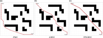
Figures 14–19 show the path diagrams and convergence curves of the three algorithms under grid map 10 * 10, 15 * 15 and 20 * 20, respectively. It can be seen from the figures that under the same maximum iteration times and initial population, the three algorithms can find a reachable path from the starting point to the target point. Among them, TPGWO algorithm has high convergence accuracy under three grid maps with different areas. In the convergence process, PSO algorithm and GWO algorithm are easy to fall into local optimization, while TPGWO algorithm can better jump out of local optimization, and can find global optimization and improve accuracy. It can be seen from the operation results in Table IV that the path selected by the TPGWO algorithm is better and the path planning takes less time. In order to avoid the occasionality of the three algorithms in the path planning, 15 different maps are generated at random for each different map size, under the condition of a certain number of obstacles. The length and running time of the path planning obtained by the three algorithms under each map are recorded, and the product of them is used to show the performance of the algorithm. As shown in the Fig. 20, horizontal axis represents the map order under certain map size and certain number of obstacles, and vertical axis represents the product of path length and running time. It can be seen from the figure that the TPGWO algorithm has good accuracy and stability in path planning under different maps. In conclusion, under the same conditions, TPGWO algorithm can find the reachable path from the starting point to the target point better, faster and more stably than PSO algorithm and GWO algorithm in the path planning of the detection robot.
Results of path planning of PSO, GWO and TPGWO under 10 * 10 grid map. (a) PSO. (b) GWO. (c) TPGWO.

Convergence curve of PSO, GWO and TPGWO for path planning under 10 * 10 grid map. (a) PSO. (b) GWO. (c) TPGWO.

Results of path planning of PSO, GWO and TPGWO under 15 * 15 grid map. (a) PSO. (b) GWO. (c) TPGWO.

Convergence curve of PSO, GWO and TPGWO for path planning under 15 * 15 grid map. (a) PSO. (b) GWO. (c) TPGWO.

Results of path planning of PSO, GWO and TPGWO under 20 * 20 grid map. (a) PSO. (b) GWO. (c) TPGWO.

Convergence curve of PSO, GWO and TPGWO for path planning under 20 * 20 grid map. (a) PSO. (b) GWO. (c) TPGWO.

Statistical results of three algorithms under different map sizes. (a) Map size 10 * 10. (b) Map size 15 * 15. (c) Map size 20 * 20.

Path length and running time of different algorithms in different map environments.

In order to verify that the convergence factor function in TPGWO algorithm in Section 4.2 can improve the convergence speed and accuracy by adjusting the parameter value, the simulation is carried out in the map of different number of obstacles. Taking the 15 * 15 grid map as an example, a simple map with fewer obstacles and a complex map with more obstacles are randomly generated. As shown in Table V, the initial population number of TPGWO algorithm
 $N\text{ is}$
30, and the maximum number of iterations
 $t_{\max }\text{ is }600$
, and the convergence factor functions are
 $a^{\prime}_{1},a^{\prime}_{2},a^{\prime}_{3}$
.
Parameter selection of TPGWO path planning.

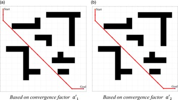
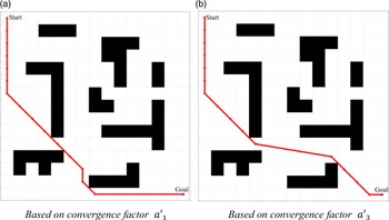
Figures 21–24 show the path diagram and convergence curve of TPGWO algorithm under three convergence factor functions. According to the graph analysis, in the simple 15 * 15 grid map with few obstacles, the same effective path can be obtained by using the convergence factor function
 $a^{\prime}_{2}$
with earlier turning points and using the convergence factor function
 $a^{\prime}_{1}$
with constant turning point, but the convergence speed of the former is faster. In the 15 * 15 grid map with more and complex obstacles, the resulting path is more accurate using the convergence factor function
 $a^{\prime}_{3}$
with slightly delayed turning point than using function
 $a^{\prime}_{1}$
. According to the data in Table VI, the convergence factor function
 $a^{\prime}_{2}$
can effectively shorten the running time of the algorithm, and the convergence factor function
 $a^{\prime}_{3}$
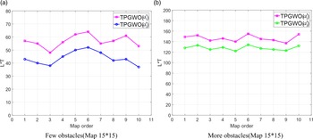
can effectively improve the accuracy of the algorithm. In order to avoid the occasionality of the path planning, two kinds of maps with different numbers of obstacles are generated. Ten different maps are generated for fewer and more obstacles, respectively. The path size and running time of different convergence factors under each map are analysed, as shown in Fig. 25, horizontal axis represents the map order, and vertical axis represents the product of path length and running time. It can be seen from the figure that adjusting the convergence factor parameters does not affect the stability of the TPGWO. Therefore, when the map area and the number of obstacles are certain, properly adjusting the turning point of the convergence factor curve according to the proportion of the number of obstacles to the map area can effectively improve the convergence speed and convergence accuracy of TPGWO algorithm in the application of patrol robot path planning.
Path planning results with convergence factor
 $a^{\prime}_{1}$
,
 $a^{\prime}_{2}$
under simple map with few obstacles. (a) Based on convergence factor
 $a^{\prime}_{1}$
. (b) Based on convergence factor
 $a^{\prime}_{2}$
.

Convergence curve of path planning with different convergence factors under simple map with few obstacles. (a) Based on convergence factor
 $a^{\prime}_{1}$
. (b) Based on convergence factor
 $a^{\prime}_{2}$
.

Path planning results with convergence factor
 $a^{\prime}_{1}$
,
 $a^{\prime}_{3}$
under a complex map with a large number of obstacles. (a) Based on convergence factor
 $a^{\prime}_{1}$
. (b) Based on convergence factor
 $a^{\prime}_{3}$
.

Convergence curve of path planning with different convergence factors on complex map with many obstacles. (a) Based on convergence factor
 $a^{\prime}_{1}$
. (b) Based on convergence factor
 $a^{\prime}_{3}$
.

Values of
 $L*T$
in TPGWO algorithm under different convergence factor functions. (a) Few obstacles (Map 15 * 15). (b) More obstacles (Map 15 * 15).

Running results with different convergence factor functions under different maps of obstacles with the same area.

The comparison of different algorithms in path planning is shown in Fig. 26. Figure 26(a) shows the path results of three algorithms under different maps, and Fig. 26(b) shows the path results of different convergence factor parameters in TPGWO algorithm under different number of obstacles under the same map size. The following conclusions can be drawn from the simulation results: (1) it is verified that TPGWO algorithm has better convergence, stability, rapidity and accuracy than PSO algorithm and GWO algorithm under the path planning of different maps; (2) it is verified that when the TPGWO algorithm is used for path planning, the parameters in the convergence factor function can be adjusted by analysing the number of obstacles in the map, thus improving the time and accuracy of path planning.
Simulation verification results.

6. Conclusion
Many algorithms can be used in path planning of inspection robot. However, different optimization algorithms have their defects and limitations in the application of path planning. In this paper, TPGWO algorithm is proposed to overcome the shortcomings of GWO algorithm in the path planning of patrol robot, such as small search range, slow convergence speed and easily falling into local optimization. TPGWO algorithm uses the idea of cross-mutation and roulette to increase the initial population number and improves the convergence factor function in GWO algorithm to a nonlinear convergence factor function that can adjust the turning point, which can not only expand the early search range but also speed up the convergence speed in the later stage to avoid falling into local optimization. At the same time, the calculated turning time and turning angle of the path are added to the fitness function of path planning to improve the accuracy of path selection. The performance of TPGWO is tested by 16 test functions. The results show that TPGWO has better convergence, stability and accuracy than PSO and GWO under the same conditions. Finally, through the path planning simulation experiment, it is found that TPGWO has better path and shorter path planning time than PSO algorithms and GWO algorithms in different map environments. At the same time, the parameters in the convergence factor function of TPGWO are adjusted according to the number of obstacles in the map. The simulation results of path planning show that adjusting the parameters in the convergence factor function properly can effectively improve the accuracy and speed of path planning. As a global path planning optimization algorithm, TPGWO has achieved good results in different map environments, but it has certain defects in local and dynamic obstacles. Therefore, in subsequent research, local optimization algorithms such as artificial potential field method and dynamic window approach can be improved and combined with TPGWO to solve such problems, so that the patrol robot can effectively avoid dynamic obstacles and complete the inspection task more accurately.
Author contributions
Qian Zhang and Yingying Li conceived and designed the study. Xucheng Ning and Lei Pan conducted programming, and Xucheng Ning performed the analyses. Qian Zhang and Xucheng Ning wrote the article and revised it according to the nice comments and suggestions from the reviewers. Rui Gao and Liyang Zhang gave necessary help during simulations and valuable suggestions on the analyses.
Financial support
This research is funded by National Natural Science Foundation of China (Grant No. 62101377) and Tianjin Municipal Education Commission Scientific Research Program Project (Grant No. 2020KJ057 and Grant No. 2018KJ176).
Conflicts of interest
The authors declare none.