




No CrossRef data available.
Did Illegal Overseas Absentee Ballots Decide the 2000 U.S. Presidential Election?
Published online by Cambridge University Press: 01 September 2004
Abstract
Although not widely known until much later, Al Gore received 202 more votes than George W. Bush on election day in Florida. George W. Bush is president because he overcame his election day deficit with overseas absentee ballots that arrived and were counted after election day. In the final official tally, Bush received 537 more votes than Gore. These numbers are taken from the official results released by the Florida Secretary of State's office and so do not reflect overvotes, undervotes, unsuccessful litigation, butterfly ballot problems, recounts that might have been allowed but were not, or any other hypothetical divergence between voter preferences and counted votes. After the election, the New York Times conducted a six-month investigation and found that 680 of the overseas absentee ballots were illegally counted, and almost no one has publicly disagreed with their assessment. In this article, we describe the statistical procedures we developed and implemented for the Times to ascertain whether disqualifying these 680 ballots would have changed the outcome of the election. These include adding formal Bayesian model averaging procedures to models of ecological inference. We present a variety of new empirical results that delineate the precise conditions under which Al Gore would have been elected president and offer new evidence of the striking effectiveness of the Republican effort to prevent local election officials from applying election law equally to all Florida citizens.The authors are deeply grateful to the many private citizens of every political stripe who sent us comments on this paper; also to Jim Alt, Barry Burden, James Honeker, Doug Rivers, and Jonathan Wand for helpful discussions; to Henry Brady for many suggestions; and to the National Science Foundation, the National Institutes of Aging, and the World Health Organization for research support. Software to implement the methods in this article is available at http://gking.harvard.edu.
Information
- Type
- SYMPOSIUM
- Information
- Copyright
- © 2004 American Political Science Association
Introduction
Many aspects of the 2000 presidential election were the subject of considerable media interest, litigation, and academic analysis during the uncertain month that followed the voting. But one aspect of the election, Florida's overseas absentee ballots, received little attention and was the object of no legal action. Yet it determined the outcome: if only the votes cast on election day were counted, Al Gore would have beat George W. Bush by 202 votes and become president. According to official results from the State of Florida, it took the overseas absentee ballots for Bush to outdistance Gore, which he did in the end by 537 votes (see table 1). The extent to which the law was followed in this small but consequential part of the story escaped scrutiny for some time. After the election was certified, however, the New York Times conducted a six-month investigation, during which it retrieved the envelopes in which the ballots were mailed and searched for violations of the law.1
In one of the longest sets of articles ever published by the Times, the news organization concluded that 680 of the overseas absentee ballots that had been counted by Florida counties unambiguously violated one or more aspects of Florida election law and, by any reasonable interpretation of the law, should have been discarded. Indeed, after the Times story appeared, commentators and partisans from both sides accepted these factual claims.2The only exception seems to have been Zelnick 2001.
Official results of the 2000 presidential election in Florida

In comparison with other features of the election that have been studied, this problem was not caused by old machines or the inattention of local election officials. It also does not rely on somehow inferring the intent of the voters. Rather, according to the Times, the overseas ballot problem was due to blatantly illegal actions on the part of local election officials, encouraged by Republicans, that had not been previously noticed. The Times argued that these local officials were influenced by the deliberate political strategies employed by the Bush campaign and by comparative neglect from the Democrats.3
The Democrats had planned to contest the absentee ballots. But Democratic Vice Presidential Candidate Joe Lieberman, appearing on Meet the Press, ended this strategy when he explained that he “would give the benefit of the doubt to ballots coming in from military personnel generally…. Al Gore and I don't want to ever be part of anything that would put an extra burden on the military personnel abroad who want to vote.” Gore backed him up and left the Republican strategy unchallenged. Berke 2001.
Ibid.
Since the partisan atmosphere surrounding public discourse on this issue was so highly charged, we knew that our work would be subject to more than the usual academic and public scrutiny and sought methods that would be least vulnerable to partisan criticism. We therefore used three separate approaches: Inference (1) with no statistical assumptions, (2) with a succession of single models that any partisan might have considered, and, finally, (3) with Bayesian model averaging, which enabled us to average over all of these single models, using weights based on the relative probability that each model is correct, as estimated from the data. So that others can use these methods to analyze similar problems, we have included all new methods introduced here in the program EI: A Program for Ecological Inference.
We estimate the probability that Gore would have won the election if the law had been followed in this instance. This probability is small, but we show that with mathematical certainty it is greater than zero. Secondly, although our results suggest that it is unlikely that illegal overseas absentee ballots alone changed the election outcome, we show that Bush's margin of victory would likely have been much narrower if those flawed ballots had not been counted. This supports the argument made by the Times that the flawed ballots favored Bush much more than Gore. We also present a variety of results that did not appear in the Times article, including the probability that Gore would have won under various hypothetical scenarios, such as if Florida Secretary of State Katherine Harris had accepted Palm Beach County's recount, which was submitted two hours late. In some plausible scenarios, the probability that Gore would have won is nearly 100 percent. Finally, and perhaps most interesting, we present evidence that the propensity of local election officials to violate the law and accept bad ballots was substantially greater in counties where Bush strategists believed there was more absentee ballot support for their candidate and tried to convince election officials to accept bad ballots. This is consistent with the Times' thesis and evidence that local election officials yielded to the will of Republican lobbyists.
Invalid Overseas Absentee Ballots in Florida
On July 15, 2001, the New York Times published “How Bush Took Florida: Mining the Overseas Absentee Vote.” The Times reporters described the details of the Bush campaign effort to secure victory by pressuring selected local election officials to count invalid overseas absentee ballots in Florida. In particular, Republicans focused on military ballots and counties where Bush had his strongest voting base. For example, in counties such as Escambia and Santa Rosa, Bush lawyers argued that every vote cast by Americans in uniform should be counted, regardless of the letter of the law. In Democratic counties, Bush's lawyers argued exactly the opposite—that local election officials must follow the letter of the law and disqualify any ballot not meeting the rules.
According to the Times, this unequal pressure led to unequal treatment by local officials of overseas voters. That partisans would pursue their interests creatively, relentlessly, and even inconsistently in different places is neither a novel claim nor remotely illegal. That local election officials would respond to this pressure by treating voters unequally is, however, a more serious claim. The Times' view—“the result was unequal treatment of ballots with the same flaws”—contradicts statements by Katherine Harris that the rules were applied uniformly.7
It also would seem to violate the Equal Protection Clause of the U.S. Constitution, which was part of the stated grounds under which the United States Supreme Court in Bush v. Gore stopped the manual recounts.The 680 ballots that the Times judged as flawed fell into one or more of the following categories:8
Ibid. Photographs of the bad ballots make the determination of flaws unambiguous; for examples, see http://www.nytimes.com/images/2001/07/15/politics/absentee/nat_ABSENTEE_count_index.html.
At times, the Republicans argued that military ballots did not need a postmark because the law allowed those in the military to send mail without postage. However, according to the Times, Florida state law clearly required overseas ballots to be “postmarked or signed and dated” by election day. Barstow and Van Natta Jr. 2001.
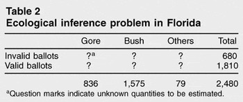
Table 2 illustrates the estimation problem at the state level. The question marks indicate the unknown quantities to be estimated. The table illustrates that while we know the aggregate number of invalid and valid ballots, as well as the total number of votes each candidate obtained from overseas absentee voters, we do not know their composition, which is the goal of the analysis. Analogous contingency tables exist for all 67 Florida counties, and the same ecological inference problem exists in each. We received three other kinds of data for each county. First, from voter registration records, we have individual-level data about overseas absentee voters, including their sex, race, party registration, and whether they were military personnel or civilians. Second, for comparative purposes, we have data available for election day voters in the 67 counties. Finally, the Times provided us indicator variables for four regions in Florida and some other measures. We use this extra information to improve our ecological inferences.
Ecological inference problem in Florida

Ecological Inference for Flawed Ballots
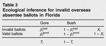
Table 3 presents our notation. For each county i (i = 1,…, 67), we denote the proportion of invalid ballots among all overseas absentee ballots as Xi and the total number of overseas absentee ballots which were counted as Ni. We let Gore's proportion of the vote be Ti. To simplify presentation, we combine the votes for Bush and the other minor candidates as Bush votes.10
Although our presentation always involves only the Bush/Gore choice, our empirical results using deterministic bounds, presented below, include the possibility of bad ballots having been cast for minor party candidates. We handle minor parties in our statistical analyses by ignoring the problem at first and then conducting sensitivity analyses in appendix B; since votes for minor party candidates only total 3 percent, we find, as expected, that they have a very small effect on the overall result. Other analyses (not shown) using more computationally intensive techniques designed to model these choices separately confirm the results. See Rosen et al. 2001.
Ecological inference for invalid overseas absentee ballots in Florida

Although βibad and βigood are used for estimation, our ultimate quantity of interest is Bush's margin after dropping the invalid absentee ballots. To define this quantity, first define the statewide fraction of bad ballots that went to Gore (βbad) as the weighted average of the individual county quantities:11
The weighted average is βbad = Σi=167Ni βibad/Σi=167Ni.

Once we estimate this quantity, we can also estimate the probability of Gore's victory, Pr(Bush's margin < 0).12
Note that βgood is not used in equation (1) but is necessary as an ancillary parameter during estimation.
Analysis without statistical assumptions
The parameters in table 3 follow an accounting identity,

that is generated by the aggregation process, and therefore always holds exactly with no stochastic term. It also implies a deterministic linear relationship between the two unknown parameters,13

that traces out what King calls a tomography line.14
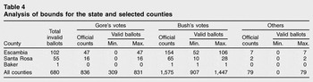
In addition, before we observe Xi and Ti in any county, we also know that βibad and βigood are each between 0 and 1. Once we observe Xi and Ti, we can narrow the bounds further by projecting the line in equation (3) to the two axes. Thus, without any statistical assumptions, we can derive the upper and lower bounds of βigood and βibad for each county i, which in turn imply the bounds for our quantity of interest, Bush's margin after dropping the flawed overseas absentee ballots.Table 4 shows how the analysis of bounds can be very powerful in some situations. For example, Escambia is one of the counties where many invalid ballots were found. At the same time, this county is one of Bush's strongholds. Seventy-six percent of the county's 208 overseas absentee ballots, or 154 votes, went to Bush, with Gore receiving 47 and 7 more cast for other candidates. Later, 102 of these ballots were deemed invalid. Because Bush had 154 total votes, it is possible that all 102 of the invalid ballots were cast for him. This produces the lower bound on the number of valid Bush votes, namely 52. The upper bound occurs when Gore and other candidates get assigned the maximum number of invalid ballots. Since Gore had 47 votes and other candidates received 7, the maximum number of invalid ballots that can be assigned to them is 54, leaving 48 invalid votes for Bush. Hence the maximum number of valid votes for Bush is his official count of 154 minus 48, or 106. Finally, Baker County illustrates why the secret ballot is sometimes not really secret. Only one absentee ballot was cast there, and it was also found to be invalid. Therefore, we know from the total tally of absentee ballots in this county—one vote for Bush—that this person voted for Bush, and that his or her ballot was invalid but included in the official count.15
Indeed, the name, address, and individual vote cast by all people in counties, like Baker, that cast all their absentee ballots for one candidate, are on the public record. This is because the bounds have zero width whenever either Xi or Ti is zero or one.
Analysis of bounds for the state and selected counties

From these county-level bounds, we derive aggregate bounds for the total number of invalid ballots for each candidate at the state level. The result shows that at least 8 percent, or 128 votes out of the 1,575 absentee ballots cast for Bush, should not have been counted; whereas the minimum number of invalid ballots for Gore is only 5 out of his total 836 votes (0.6 percent). Furthermore, Bush could have inappropriately benefited from up to 668 out of the 680 invalid ballots.
The most significant conclusion from this analysis is that we cannot exclude the possibility that Gore actually won the election. That is, without making any assumptions other than that the Times coding decisions were correct (and again, we saw no significant objection to them in the media discussion that followed their story), the 537 vote margin for Bush now changes to somewhere from a 126 vote victory for Gore to a 936 vote victory for Bush. However, once the ballots were removed from the envelopes, America forever gave up the possibility of knowing for certain who won the most votes in Florida's 2000 election.
Statistical analysis with a single model specification
The lack of any statistical assumptions puts the analysis presented in the preceding section on firm footing. In fact, measurement error aside, its conclusions contain no inferential uncertainties at all (which is quite unusual for social science research). If the resulting bounds excluded the chance of one candidate winning, our analysis would end here. Unfortunately, the bounds only reveal that there exists a possibility that either Gore or Bush received more votes. Indeed, even if all but a tiny piece of the bounded interval reflected a Bush (or a Gore) victory, it would provide no information about the probability that a particular candidate won other than that zero is excluded (since the bounds alone do not imply any probability distribution over the interval). Since this probability was the quantity of interest for our project, the Times reporters needed us to go further than the bounds. They needed us to make an inference about the probability that around 90 percent of the bad ballots went to Bush, which, if true, would have produced a Gore victory.
To learn more about who actually won the Florida election—the likely margins of victory within the deterministic bounds—the only option is to add some statistical assumptions. With them, we can make probabilistic statements about our quantities of interest. The problem with any model-based statistical analysis, of course, is that there might be disagreement about the assumptions to be made. The price we must pay for the more precise results that follow is the additional uncertainty due to model specification. This is a common problem in social science research, but it is particularly salient when attempting to provide independent, nonpartisan advice in the midst of one of the most highly charged partisan debates in modern times. Our approach to this problem is to formally incorporate uncertainty due to model specification into our final estimate.
We use the class of ecological inference models (now called EI after the software that implements them) given in King's A Solution to the Ecological Inference Problem.16
The choices of models within this class have been contested in specific applications since, as with any ecological inference technique, models require identifying assumptions that may or may not be appropriate.17See, for example, Adolph and King 2003; Adolph et al. 2003; Anselin and Cho 2002a; Anselin and Cho 2002b; Cho 1998; Cho and Gaines 2004; Freedman et al. 1998; Herron and Shotts 2003a; Herron and Shotts 2003b; King 1999; King 2002.
On parametric and nonparametric advances see Imai and Lu 2004. See also King, Rosen, and Tanner 2004, which includes methodological developments in ecological inference from contributors in many academic disciplines.
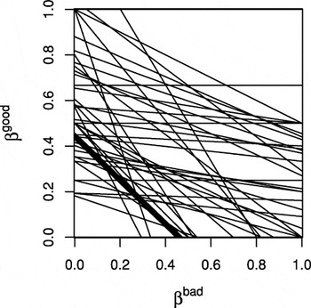
To begin, we summarize graphically the bounds obtained above. For each Florida county, we show all possible values of βibad and βigood. As it turns out, the data tell us more than merely the bounds on each parameter separately since equation (3) says that if βigood is near the top of its bounds, βibad must be near the bottom of its bounds. In fact, the two are perfectly correlated and fall on a line defined by that equation. To illustrate, we chart one line for each county in Florida in the tomography plot of figure 1, which merely reexpresses the data in the form closest to the answers we seek. This is as far as it is possible to go without making statistical assumptions. Next, we add three assumptions, all conditional on X and a specified set of control variables Z. We could begin with the assumption that βibad and βigood are the same for all counties, which is essentially Goodman's regression.19
This would be enough to identify the model, but it would be a very strong assumption, and indeed in our application it can be rejected with certainty by merely examining figure 1.
Tomography plot for invalid overseas absentee ballots. %βibad and βigood are the proportion of Gore's invalid and valid ballots, respectively. Each line traces out the possible values of the βibad, βigood point for each county i. The thick solid line represents Escambia County.
Thus, instead of assuming that βibad and βigood are the same over counties, we assume that they come from the same distribution (the truncated bivariate normal distribution, with truncation kept to the square in the figure). The idea is that whatever the values of the unknown parameters from Florida's 67 counties on their respective tomography lines, they all have something in common—since they are all in the same state, subject to almost the same electoral campaign, et cetera. Differences of any size across the counties in these parameters are therefore allowed so long as they are either random and fit the distributional assumption, or they are systematic and taken into account by control variables. The main constraints added by this assumption are that the bivariate density is unimodal (which is the formalization of the assumption that the counties “have something in common”) and that all volume under the density appears over the square represented by the tomography plot. Violations of this distributional assumption do not seem to affect the quantities we need for this application.20
King 1997, table 9.2.
The second assumption is the absence of residual spatial correlation in T after taking into account X and Z. King's ecological inference model has been shown to be relatively insensitive to anything but extreme levels of spatial autocorrelation,21
Ibid., table 9.1; King 2000.
The final assumption states that the two unknown quantities, βibad and βigood, are independent of Xi, given Z. For example, if more bad ballots cast for Gore, βibad, came from counties with more bad ballots overall, Xi, then this assumption would be violated unless Z included variables that sufficiently controlled for this relationship. This is the most critical of the three assumptions, and so the validity of the analysis depends on the content of Z. Each of these three assumptions can be modified or relaxed by the inclusion of different covariates, Z, and so the main model uncertainty that is assumed presently is Z.
Statistical analyses that acknowledge model uncertainty
Sensitivity to model specification in quantitative political science is perhaps most commonly seen when minor changes among the explanatory variables in regression-type analyses result in large differences in the estimates. The endemic nature of such model dependent inferences makes a decision to base inferences on a single model highly dubious in many situations. This is particularly true in ecological inference, where model dependence is frequently an issue. Yet, almost all existing applications of ecological inference use a single specification. Indeed, few use any explanatory variables, Z, at all.
The partisan nature of the controversy in which we were providing advice makes the issue of model dependence especially salient, although its nature is not markedly different from other applications. We began by following the most common procedure of estimating many models (i.e., with different Z) and assessing the degree to which our ultimate quantities of interest depend on the specification. This was informative but insufficient, since our task was to provide a single inference with a point estimate and confidence interval.
Three basic ways of drawing a single inference in the presence of model uncertainty exist. Some researchers persist in choosing a single model, perhaps on the basis of qualitative arguments about its merits, and draw inferences assuming its veracity. This optimistic approach often overestimates the degree to which the researcher is certain of the correct model specification, and hence typically gives biased estimates and overly narrow confidence intervals. Other researchers use a formal model selection criterion, such as stepwise regression, Mallow's Cp, or AIC, to pick the best model. Although these procedures are inappropriate when estimating causal effects, they are reasonable when the quantity of interest is predictive, such as ecological inference. Unfortunately, even in these situations, the result of applying these criteria is one model, which also ignores model uncertainty.
An approach now widely recognized to be superior to standard model selection criterion is Bayesian model averaging, which we apply to our ecological inference problem. The basic idea is to estimate a large number of potential models and take the weighted average of their results, with weights based on the probability that a model is correct. The correctness of the model is not assumed ex ante, nor is it merely based on goodness of fit; it is instead calculated from the data via Bayesian analysis. The key result of Bayesian model averaging is that the resulting inferences (1) are more accurate than those produced by standard model selection criterion, (2) formally incorporate model uncertainty, and (3) outperform any of the individual models that are averaged over. The last property does not depend on whether the true model generating the data lies inside or outside models averaged over. That is, inferences from Bayesian model averaging always outperform any individual model considered.22
E.g., Madigan and Raftery 1994. This result is similar to insights from the closely related literature on committee methods, although surprisingly the literatures have relatively few cross-citations. Bishop 1995; see also Rosen, Jiang, and Tanner 2000; and Robert 1996. See Hoeting et al. 1999 for a general introduction to Bayesian model averaging. Raftery and Zheng 2003 derive the optimality of its long-run performance. See Bartels 1997; Bartels and Zaller 2001; and Erikson, Bafumi, and Wilson 2001 for political science applications that use an approximation to formal Bayesian model averaging.
Of course, one can never cover the entire model space, which is normally of infinite size, since Bayesian model averaging only allows one to include a finite number of models. Therefore, the resulting inferences can always be improved by adding additional models, no matter how many models have already been included. This is not a unique feature of Bayesian model averaging since it is always possible to come up with a better model for any statistical analysis where the correct model is unknown to researchers. However, Bayesian model averaging offers a significant improvement over the usual approach of basing inferences on one assumed model, no matter how that model is chosen.
Bayesian model averaging is especially important in our application since political scientists have rarely studied absentee ballots, and we therefore have little prior theory with which to assist in model specification. The procedure thus enables us to conduct an analysis without having to defend one particular specification, or even a small set of specifications. We came up with our list of models by talking in detail to reporters and partisans on both sides. We then formalized their intuitions into an ecological inference model (by defining Z) and included every one in our analysis. We also added several other models we came up with independently.
Our search for models identified 31 possibilities for Z, including the race, sex, and party registration of overseas absentee voters as well as models based on 24 county-level election and demographic variables. We also include a model with no covariates, and three models with Xi as the covariate for the mean of βbad, βgood, and for both.23
A list of all 31 models follows: (1) no covariate, (2) Xi for βbad, (3) Xi for βgood, (4) Xi for both βbad and βgood, (5) military absentee voters, (6) registered Republican absentee voters, (7) registered Democratic absentee voters, (8) female absentee voters, (9) White absentee voters, (10) black absentee voters, (11) Hispanic absentee voters, (12) rejected military absentee voters, (13) rejected registered Republican absentee voters, (14) rejected registered Democratic absentee voters, (15) rejected female absentee voters, (16) rejected white absentee voters, (17) rejected black absentee voters, (18) rejected Hispanic absentee voters, (19) Democratic vote share among residents, (20) vote share of Republican candidates, (21) vote share of other candidates, (22) registered Democratic residents, (23) registered Republican residents/registered black Democratic residents, (24) proportion of voting age population not registered, (25) black registered Democrats, (26) black registered Republican residents, (27) acceptance ratio of overall absentee ballots, (28) ratio of invalid absentee ballots, (29) Panhandle Florida regional indicator variable, (30) southern Florida regional indicator variable, (31) corruption indicator. All the covariates except indicator variables are entered as a ratio varying from 0 to 1. Except the first three models, the covariate was used to model the conditional untruncated mean of both parameters, βbad and βgood. Models (5) to (11) are based on information about the absentee ballots, so different variables were available regarding the invalid and valid ballots; we used the former group to predict βbad and the latter to predict βgood. We reran each model with different starting values to verify that we found the global maximum. We also examined each of the tomography plots with confidence regions to search for outliers or bad model fits. In addition, we plotted E(T |X) or E(T |X,Z) by X or Z, and checked whether the observed T fell within the (say) 90 percent confidence interval 90 percent of the time.
Multiple covariates uncorrelated with Xi cause no identification problems in EI. Ecological inference models that do not incorporate information from the deterministic bounds are not identified when including Xi or variables related to X. See Goodman 1953; King 1997. Thus, to the extent that models that incorporate the bounds, such as EI, are estimable when including Xi or covariates that are related to Xi, the information that makes this possible is coming from the bounds. Predictions about the quantities of inferences in EI are not often greatly affected by including more than one covariate at a time.
Although we know of no application of ecological inference that uses more than a single explanatory variable (and almost all applications use none), we also tried expanding our setup from 0, 1, and 2 variable models to ones that include several 3 and 4 variable specifications. While some of these highly computationally intensive models had large enough estimated weights to be meaningful, including them in the Bayesian model averaging procedure did not appreciably change our substantive estimates. Of course, we have also omitted an infinite number of other possible models from the set we average over, and it is possible that future researchers will find and include a model we excluded that would change our empirical conclusions. For example, we exclude all models with more than four explanatory variables, as well as all interactions and all models based on data we do not have. Our Bayesian model averaging results are known to be better than any individual model among those we average over; but our results could be overturned if someone finds a plausible model to add that has a high probability of being correct and leads to different inferences.
Empirical Results
Would Gore have won the election without the bad ballots? In this section we discuss that possibility, as well as a variety of more specific counterfactuals, and evidence about how local election officials differentially responded to Republican pressure in their application of local election law.
The probability that Gore would have won without bad absentee ballots
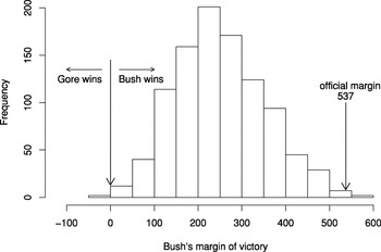
Figure 2 portrays the posterior distribution from our analysis of Bush's margin of victory if the bad ballots had not been counted (the histogram of 1000 draws from the posterior). Note first that, as required by the procedure, all area for this distribution is contained within the bounds we found for this quantity of −126 to 936. The weight of the statistical evidence within these bounds clearly demonstrates that Bush benefited from the bad ballots, and that removing them takes away from his margin. This is evident in the figure because almost all of the area of the histogram of posterior probability falls to the left of the official margin of 537 votes. The mean margin of victory for Bush without the bad ballots is only 251 votes. The figure also portrays the probability that Gore actually won the election by the area under the curve to the left of zero. This is only about 0.2 percent, indicating that Gore probably would not have won, even if the bad ballots had been discarded.

Posterior distribution of Bush's margin of victory without the 680 invalid overseas absentee ballots.
Other counterfactuals
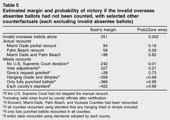
While our results indicate that it is unlikely that invalid overseas absentee ballots alone changed the election outcome, the illegally counted ballots could have had a much more significant effect when combined with slight changes in decisions regarding the manual recounts. We show this result by first focusing on several scenarios involving the two key counties where a manual recount was conducted—Miami Dade and Palm Beach. In Miami Dade County, election officials decided to stop the manual recount when they determined that they could not meet the deadline set by the Florida Supreme Court, 5 pm Sunday, November 27. Their partial manual recount gave a net gain of 157 votes to Gore. Officials in Palm Beach County also concluded that they could not finish the manual recount in time. But while they submitted the outcome of their partial recount just before the deadline—a net gain of 192 votes for Gore—they also reported the result of the complete recount to Katherine Harris later that day. She, however, rejected this complete recount as well as the two partial recounts and did not include them in the certified official tally, thereby denying Gore a total of 349 votes.27
The panel of table 5 marked “actual recounts” presents our prediction for Bush's margin and Gore's probability of victory in situations where the invalid overseas absentee ballots had been rejected and the recounts in one or both of these counties had been included in the final tally. For example, if the recounted votes in Miami Dade and Palm Beach had all been counted, Gore would have won with a 0.82 probability, with the uncertainty in this number coming only from our analysis of the bad overseas absentee ballots. If only the Palm Beach votes had been counted, Gore would have won with a 0.29 probability. To put it one way, the massive differences in the probabilities from 0.002 to 0.82 for a Gore victory were due to the decisions made by Katherine Harris. Of course, these decisions could have been overturned by the courts, and the candidates could have influenced them if they had requested statewide or different types of recounts.
Estimated margin and probability of victory if the invalid overseas absentee ballots had not been counted, with selected other counterfactuals (each excluding invalid absentee ballots)

In the last panel of table 5, we consider counterfactuals where the invalid overseas absentee ballots had not been counted and election day voting recounts had occurred in various ways, as suggested in a study conducted by a consortium of media organizations.28
For instance, this analysis shows that if the U.S. Supreme Court had not stopped the recount in Bush v. Gore, the victor would have changed with only a 1 percent probability. However, if Gore's formal request that Broward, Miami Dade, Palm Beach, and Volusia Counties be recounted had been granted, he would have been elected with a 73 percent probability. If the entire state had been recounted, according to almost any standard for judging the punch cards, Gore would have won the election with a very high probability.Indirect evidence of local election officials responding to Republican pressure
Six months of interviews and archival research in Florida and elsewhere led reporters from the New York Times to conclude that “the Republicans mounted a legal and public relations campaign to persuade canvassing boards in Bush strongholds to waive the state's election laws when counting overseas absentee ballots…. Their goal was simple: to count the maximum number of overseas ballots in counties won by Mr. Bush, particularly those with a high concentration of military voters, while seeking to disqualify overseas ballots in counties won by Vice President Al Gore.”29
The Times claimed that, as a direct result of this pressure,
[C]anvassing boards in about a dozen Republican-leaning counties had reconvened for a second round of counting. In each place, longstanding election rules were bent and even ignored. Boards counted ballots postmarked as many as seven days after the election, including some from within the United States. They counted two ballots sent by fax. Officials in Santa Rosa County even counted five ballots that arrived after the November 17 deadline. Again and again, election officials crossed out the words “REJECTED AS ILLEGAL” that had been stamped on ballot envelopes.30
Ibid., 16.
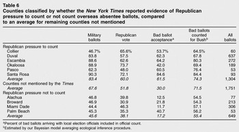
If these claims are correct, we ought to be able to find evidence of them in our data. We therefore conducted two tests. In the first, we divide Florida's counties into three categories: the six counties mentioned explicitly in the Times story where the Republicans pressured officials to count illegal ballots, the four counties mentioned where Republicans pressured local election officials not to count the ballots, and the remaining counties that were not mentioned. We then compute various statistics for these three categories and present them for comparison in table 6. (The results in this table were not available to the reporters before their article appeared, so table 6 does represent an independent test.)
Counties classified by whether the New York Times reported evidence of Republican pressure to count or not count overseas absentee ballots, compared to an average for remaining counties not mentioned

The evidence strikingly supports the Times' account of events. The first two columns of table 6 report on the characteristics of the county, information available to Republican strategists before they started lobbying. With the exception of two counties with very few absentee ballots, the ones identified as areas where the Republicans focused their efforts to count ballots were those with large populations of military personnel and Republican voters. Similarly, counties that the Times identified as places where Republicans discouraged the ballots from being counted had consistently fewer military personnel and Republican voters.
The result of the Republican efforts also appears to have been successful. A larger fraction of bad ballots were counted in those counties where Republicans tried to get them accepted than the average, and a smaller fraction than the average were counted in every county where the Republicans tried to have them rejected. The fraction of accepted bad ballots that had been cast for Bush supports the same theory: fewer had been for Bush where the Republicans tried to have them rejected than in every county where the Republicans tried to have them accepted.
The Times' report also helps explain some interesting variations in this table. In Duval County, for example, we would have expected to find more Bush votes among the bad ballots than we actually found, due to its large percentage of military personnel. However, the Times reported that an election official on the Duval County canvassing board “held the line on counting ballots with missing postmarks.”31
Ibid.
Ibid.
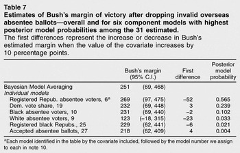
We also look for indirect evidence of local election officials succumbing to pressure from representatives of the Republican Party by examining the posterior probabilities of each of the 31 component models we included. Generally, if the Times' hypothesis is right, we would expect that the covariates that have the biggest effects would be related to areas where Republicans tried hardest to influence local officials. These would be counties that the Republicans—if they were as rational and deliberate as the Times suggested—expected to find the largest numbers of bad ballots that, if counted, would help Bush's cause. Obviously, we have no such variable, but we do have a variety of related variables. Table 7 gives the top six models listed in order of the posterior probability of being correct. The two with the largest effects are consistent with the theory that the more absentee voters registered as Republicans, and the more white absentee voters in a district, the more bad ballots cast for Bush. (The negative sign indicates that Bush's lead is reduced when these ballots are not counted.) The other covariates have comparatively small effects.
Estimates of Bush's margin of victory after dropping invalid overseas absentee ballots—overall and for six component models with highest posterior model probabilities among the 31 estimated. %The first differences represent the increase or decrease in Bush's estimated margin when the value of the covariate increases by 10 percentage points.

The large variation in our prediction for Bush's margin across the six models in table 7 emphasizes a clear advantage of our Bayesian model averaging procedure. The variation results from the large degree of model dependence in these data (because the data have fairly wide bounds). For example, the specification with white absentee voters gives a confidence interval which, when considered in isolation from the other models, would not enable us to reject the hypothesis that Gore would have won if only the overseas absentee ballots had been rejected. This is obviously quite different from our overall result of only a 0.2 percent probability that Gore won. Since different specifications yield very different inferences, an analyst having to choose one model would be in the untenable position of having to defend choices without much prior evidence.
Bayesian model averaging offers a way around this common problem. Instead of results jumping dramatically from one specification to the next, inferences resulting from Bayesian model averaging do not change as much when new models are added to the specification, unless they have especially large probabilities of being true. Of course, we cannot get something for nothing. Our procedure is an improvement over straight EI because we only need to assume that one of our 31 models, or some combination of our 31 models, contains something close to the right model. This is in contrast to the usual approach where we merely get one model from which to choose, but it is not a panacea: if someone comes up with a new idea for a model, we can include it; but if none or no combination of those we consult comes close to the right model, then our procedure will obviously fail to give valid answers.
Concluding Remarks
Counterfactual analysis is difficult, especially when the subject of the inference is far from the factual evidence. When the counterfactual is very close to the data, however, we stand a good chance of making valid inferences.33
In the case of the presidential elections in Florida, the counterfactuals are especially clear and could easily have happened, which makes the results of this particular study somewhat more certain than usual. If the problem of the overseas absentee ballots had been litigated and the law applied equally in every county (as Bush v. Gore required of the votes cast on election day), the bad ballots might very well have been disqualified. Although Gore probably still would have lost the Florida vote, we conclude that no one will ever be able to say with certainty who would have won the American presidential election. Also, if Florida's secretary of state had held different views on issues that were somewhat open to discretion, the outcome of the election might very well have changed. Of course, had the candidates expressed different views on campaign spending, Elian Gonzales, or any of a variety of other issues, the outcome might have been different. Our results also provide indirect but strong and independent support for the thesis that local election officials yielded to the efforts of Republican strategists to follow the law in Gore counties but disregard it in Bush areas.Finally, we believe this article provides an especially good example of the use of Bayesian model averaging. We have developed an application of it to the ecological inference model and offer computer code for others to use. In applied work, Bayesian model averaging has been approximated, as, for example, with the Bayesian information criteria (BIC), but its full version has not seen as much use as it could—and none before this in political science. Bayesian model averaging is a clear improvement on the usual situation, which entails having to select and defend a single model, but it is no panacea. A researcher never knows whether all relevant models have been included and, although its results are more robust than single-model approaches, it is always possible to come up with a different list of models and produce different results. And so in the end, as always, the investigator's judgment plays an important role in making inferences. Model averaging cannot substitute for judgment, but it can help account for model uncertainties where prior knowledge is not available. In the present case, where 100 percent confidence intervals are available (in the form of bounds on the parameters), we have additional constraints on possible results.
Appendix A: Technical Issues in Modeling and Estimation
From one application of one specification of this model, we compute the posterior density of a quantity of interest Δ by drawing it from its posterior, conditional on the model P(Δ|Mk,T). To do this, we draw simulations of βbad and βgood from their posterior and calculate simulations of Δ. Bayes' theorem specifies that the posterior is proportional to the product of the prior times the likelihood, P(Θ|T) ∝ P(Θ)P(T |Θ), where P(Θ) is the prior probability distribution on some unknown parameter Θ, and P(T |Θ) is the likelihood. Everything is conditioned on X, N, and Z, which we observe. We use the standard independent prior on each parameter of Θ as described in King.34
This prior distribution and the likelihood function together to define King's model in a standard Bayesian framework.Let Mk denote the kth model specification (k = 1, … , 31). Then we make an inference about a quantity of interest Δ by computing its posterior distribution via Bayesian model averaging. To do this, we first compute, for each model, the posterior distribution of Δ (computed from the posterior with Δ being some known function of Θ): P(Δ|Mk,T). Then we average over these models by weighting by the relative posterior probability that each model is correct given the data, Pr(Mk|T): Pr(Δ|T) = Σk=131P(Δ|Mk,T) Pr(Mk|T), where the posterior model probability is Pr(Mk|T) = P(T |Mk) × Pr(Mk)/[Σj=131Pr(T |Mj) Pr(Mj)]. This is the probability that model k is correct, given the set of models in the analysis; it should not be confused with R2-like measures, which typically reward models that over-fit without distinguishing systematic from idiosyncratic features of the data.
To compute the posterior model probability, we need two elements. The first is a prior probability that each model is correct, Pr(Mk), which we set to uniform. The other is the marginal likelihood, P(T |Mk), which is obtained by averaging the likelihood over the prior distribution.35
The marginal likelihood is P(T |Mk) = ∫P(T |Θk, Mk) ×P(Θk|Mk)dΘk, where P(Θj |Mj) is the prior distribution for the parameter vector Θ in Model k.
Kass and Raftery 1995, 776.
To compute the marginal likelihood, we use the Laplace approximation, which is known to perform well compared with other methods.37
Raftery 1996; Lewis and Raftery 1997; DiCiccio et al. 1997. If a model is estimated through a Markov chain Monte Carlo simulation, one can construct an algorithm where the chain visits each model stochastically and can thus compute the posterior model probability as a direct output of the posterior draws. See Chib 1995. However, this requires constructing a new MCMC algorithm for each application.
Kass and Raftery 1995, 778.
Appendix B: The Minor Effects of Minor Candidates and Prior Densities
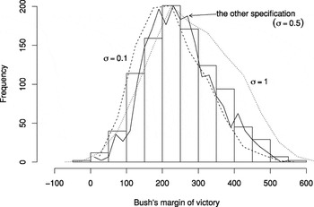
Here, we analyze the effects on our results of ignoring the minor party candidates and study the sensitivity of our results to our choices for model priors. Figure 3 plots the posterior distribution of Bush's new margin without invalid overseas absentee ballots for different model specifications in comparison to our posterior distribution. The solid line in this figure is an alternative specification of the ecological inference model where we combine the votes for the minor candidates together with those for Gore rather than with the votes for Bush, resulting in 31 new individual models corresponding to the 31 models already run. The posterior distribution for this model is very similar to the results of our previous analysis, indicating that our results do not depend on which model specification is used. The other two lines represent the use of different prior distributions for the coefficients of the covariate of each model. We use different prior standard deviations for the coefficients of the covariates to see if the results are sensitive to the choice of the prior distribution. While some features of the posterior do vary across specifications, the graph shows that model results are not particularly sensitive to the prior specification. The median posterior point in particular hardly changes across the models.

Sensitivity analysis of Bayesian model averaging. %The histogram is the posterior distribution of Bush's new margin for our model. The other lines give posterior distributions from different models and prior specifications.
References
REFERENCES
Adolph, Christopher, and
Gary King.
2003.
Analyzing second-stage ecological regressions: Comment on Herron
and Shotts.
Political Analysis
11 (1):
65–76.Google Scholar
Adolph, Christopher, and
Gary King,
with Michael C. Herron, and
Kenneth W. Shotts.
2003.
A consensus on second-stage analyses in ecological inference models.
Political Analysis
11 (1):
86–94.Google Scholar
Anselin, Luc, and
Wendy K. Tam Cho.
2002a.
Spatial effects and ecological inference.
Political Analysis
10 (3):
276–97.Google Scholar
Anselin, Luc, and
Wendy K. Tam Cho
2002b.
Conceptualizing space: Reply.
Political Analysis
10 (3):
301–3.Google Scholar
Barbanel, Josh.
2001.
How the ballots were examined.
New York Times,
July 15. http://www.nytimes.com/.
Barstow, David, and
Don Van Natta Jr.
2001.
How Bush took Florida: Mining the overseas absentee vote.
New York Times,
July 15. http://www.nytimes.com/.
Bartels, Larry M.
1997.
Specification uncertainty and model averaging.
American Journal of Political Science
41 (2):
641–74.Google Scholar
Bartels, Larry M., and
John Zaller.
2001.
Presidential vote models: A recount.
PS: Political Science and Politics
33 (1):
9–20.Google Scholar
Berke, Richard L.
2001.
Lieberman put Democrats in retreat on military vote.”
New York Times,
July 15. http://www.nytimes.com/.
Bishop, Christopher M.
1995.
Neural Networks for Pattern Recognition.
Oxford:
Oxford University Press.
Chib, Siddhartha.
1995.
Marginal likelihood from the Gibbs output.
Journal of the American Statistical Association
90 (432):
1313–21.Google Scholar
Cho, Wendy K. Tam.
1998.
Iff the assumption fits …: A comment on the King ecological
inference solution.
Political Analysis 7:
143–63.Google Scholar
Cho, Wendy K. Tam, and
Brian J. Gaines.
2004.
The limits of ecological inference: The case of split-ticket
voting.
American Journal of Political Science
48 (1):
152–71.Google Scholar
DiCiccio, Thomas J.,
Robert E. Kass,
Adrian E. Raftery, and
Larry Wasserman.
1997.
Computing Bayes factors by combining simulation and asymptotic
approximations.
Journal of the American Statistical Association
92 (439):
903–15.Google Scholar
Duncan, Otis Dudley, and
Beverly Davis.
1953.
An alternative to ecological correlation.
American Sociological Review
18 (6):
665–66.Google Scholar
Erikson, Robert S.,
Joseph Bafumi, and
Bret Wilson.
2001.
Was the 2000 presidential election predictable?
PS: Political Science and Politics
34 (4):
815–19.Google Scholar
Fessenden, Ford, and
John M. Broder.
2001.
Study of disputed Florida ballots finds justices not cast the
deciding vote.
New York Times,
November 12.
Freedman, David A.,
Stephen P. Klein,
Michael Ostland, and
Michael R. Roberts.
1998. Review of
A solution to the ecological inference problem.
Journal of the American Statistical Association
93 (December):
1518–22.Google Scholar
Goodman, Leo.
1953.
Ecological regressions and the behavior of individuals.
American Sociological Review
18 (6):
663–64.Google Scholar
Goodman, Leo
1959.
Some alternatives to ecological correlation.
American Journal of Sociology
64 (6):
610–24.Google Scholar
Herron, Michael C., and
Kenneth W. Shotts.
2003a.
Using ecological inference point estimates as dependent variables
in second-stage linear regressions.
Political Analysis
11 (1):
44–64.Google Scholar
Herron, Michael C., and
Kenneth W. Shotts
2003b.
Cross-contamination in EI-R: Reply.
Political Analysis
11 (1):
77–85.Google Scholar
Hoeting, Jennifer A.,
David Madigan,
Adrian E. Raftery, and
Chris T. Volinsky.
1999.
Bayesian model averaging: A tutorial.
Statistical Science
14 (4):
382–417.Google Scholar
Imai, Kosuke, and
Ying Lu.
2004.
Parametric and nonparametric Bayesian modeling for ecological inference
in 2 × 2 tables.
Technical report,
Department of Politics, Princeton University.
Kass, Robert E., and
Adrian E. Raftery.
1995.
Bayes factors.
Journal of the American Statistical Association
90 (430):
773–95.Google Scholar
Kass, Robert E.,
Luke Tierney, and
Joseph B. Kadane.
1989.
Approximate methods for assessing influence and sensitivity in
Bayesian analysis.
Biometrika
76 (4):
663–74.Google Scholar
King, Gary.
1997.
A solution to the ecological inference problem: Reconstructing
individual behavior from aggregate data.
Princeton:
Princeton University Press.
King, Gary
1999.
The future of ecological inference research: A reply to Freedman et
al.
Journal of the American Statistical Association
94 (March):
352–55.Google Scholar
King, Gary
2002.
Isolating spatial autocorrelation, aggregation bias, and
distributional violations in ecological inference.
Political Analysis
10 (3):
298–300.Google Scholar
King, Gary,
Ori Rosen, and
Martin A. Tanner, eds.
2004.
Ecological inference: New methodological strategies.
New York:
Cambridge University Press.
King, Gary, and
Langche Zeng.
2001.
When can history be our guide? The pitfalls of counterfactual
inference.
http://gking.harvard.edu.
Lebow, Richard Ned.
2000.
What's so different about a counterfactual?
World Politics
52 (4):
550–85.Google Scholar
Lewis, Steven M., and
Adrian E. Raftery.
1997.
Estimating Bayes factors via posterior simulation with the
Laplace-Metropolis estimator.
Journal of the American Statistical Association
92 (438):
648–55.Google Scholar
Madigan, David, and
Adrian E. Raftery.
1994.
Model selection and accounting for model uncertainty in graphical
models using Occam's window.
Journal of the American Statistical Association
89 (428):
1535–46.Google Scholar
Purdum, Todd S.
2000.
Counting the vote: The overview.
New York Times,
November 27. http:// www.nytimes.com/.
Raftery, Adrian E.
1996.
Hypothesis testing and model selection. In
Markov chain Monte Carlo in practice: Interdisciplinary statistics,
ed.
W. R. Gilks,
S. Richardson, and
D. J. Spiegelhalter,
163–87.
London:
Chapman and Hall.
Raftery, Adrian E., and
Yingye Zheng.
2003.
Discussion: Performance of Bayesian model averaging.
Journal of the American Statistical Association
98 (464):
931–38.Google Scholar
Robert, C. P.
1996.
Mixtures of distributions: inference and estimation. In
Markov chain Monte Carlo in practice: Interdisciplinary statistics,
ed.
W. R. Gilks,
S. Richardson, and
D. J. Spiegelhalter,
441–64.
London:
Chapman and Hall.
Rosen, Ori; Wenxin Jiang,
Gary King, and
Martin A. Tanner.
2001.
Bayesian and frequentist inference for ecological inference: The
R × C case.
Statistica Neerlandica
55 (2):
134–56.Google Scholar
Rosen, Ori,
Wenxin Jiang, and
Martin A. Tanner.
2000.
Mixtures of marginal models.
Biometrika
87 (2):
391–404.Google Scholar
Zelnick, Bob.
2001.
The myth of a stolen election (letter to the editor).
Wall Street Journal,
July 17.

Official results of the 2000 presidential election in Florida
Ecological inference problem in Florida
Ecological inference for invalid overseas absentee ballots in Florida
Analysis of bounds for the state and selected counties
Tomography plot for invalid overseas absentee ballots. %βibad and βigood are the proportion of Gore's invalid and valid ballots, respectively. Each line traces out the possible values of the βibad, βigood point for each county i. The thick solid line represents Escambia County.
Posterior distribution of Bush's margin of victory without the 680 invalid overseas absentee ballots.
Estimated margin and probability of victory if the invalid overseas absentee ballots had not been counted, with selected other counterfactuals (each excluding invalid absentee ballots)
Counties classified by whether the New York Times reported evidence of Republican pressure to count or not count overseas absentee ballots, compared to an average for remaining counties not mentioned
Estimates of Bush's margin of victory after dropping invalid overseas absentee ballots—overall and for six component models with highest posterior model probabilities among the 31 estimated. %The first differences represent the increase or decrease in Bush's estimated margin when the value of the covariate increases by 10 percentage points.
Sensitivity analysis of Bayesian model averaging. %The histogram is the posterior distribution of Bush's new margin for our model. The other lines give posterior distributions from different models and prior specifications.
 You have
Access
- 31
- Cited by