1. Introduction
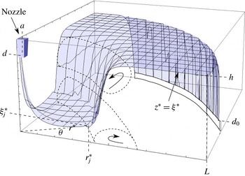
When a jet of liquid impacts upon a rigid surface, a circular ring defines the geometrical place where the hydraulic jump occurs. It is called a hydraulic jump owing to the abrupt change in the height of the fluid from the supercritical region to the subcritical region, and it has been widely studied in rectangular Cartesian coordinates (Chanson Reference Chanson2009). The terms super- and subcritical (alternatively super- and subsonic) refer to the relative magnitudes of the flow speed and wave speed in each area (see figure 1). In the supercritical region, the speed of the fluid is greater than that of the waves at the surface, and thus no information is transmitted against the stream and all the surface waves travel downstream with different speeds depending on the initial conditions. In the subcritical region, the fluid flow is slower than the surface waves, and thus information can be transmitted upstream and downstream following the Galileo velocity summation law.
In a cylindrical geometry, different types of hydraulic jumps have been reported, from turbulent (Liu, Lienhard & Lombara Reference Liu, Lienhard and Lombara1991; Arakeri & Rao Reference Arakeri and Rao1996), to steady circular (Tani Reference Tani1949; Bohr, Dimon & Putkaradze Reference Bohr, Dimon and Putkaradze1993; Hansen et al.
Reference Hansen, Hørluck, Zauner, Dimon, Ellegaard and Creagh1997; Brechet & Néda Reference Brechet and Néda1998; Rao & Arakeri Reference Rao and Arakeri2001; Bush & Aristoff Reference Bush and Aristoff2003; Kate, Das & Chakraborty Reference Kate, Das and Chakraborty2007) and polygonal jumps (Ellegaard et al.
Reference Ellegaard, Hansen, Haaning, Hansen, Marcussen, Bohr, Hansen and Watanabe1998, Reference Ellegaard, Hansen, Haaning, Hansen, Marcussen, Bohr, Hansen and Watanabe1999; Bush, Aristoff & Hosoi Reference Bush, Aristoff and Hosoi2006; Martens, Watanabe & Bohr Reference Martens, Watanabe and Bohr2012). Mathur et al. (Reference Mathur, DasGupta, Selvi, John, Kulkarni and Govindarajan2007) found gravity-free circular hydraulic shocks produced by surface tension in scales ranging from nanometres to micrometres, and Duchesne et al. (Reference Duchesne, Savaro, Lebon, Pirat and Limat2013) explore the dynamics of a drop placed on the free surface at the supersonic region. Circular jumps have been classified by the number of rolls found in azimuthal cross-sections. The type I jump consists of one recirculation vortex (see figure 1). The transition from circular to polygonal jumps is characterized by the appearance of a second surfing roll. These are called type II jumps (Bohr et al.
Reference Bohr, Ellegaard, Hansen and Haaning1996; Ellegaard et al.
Reference Ellegaard, Hansen, Haaning and Bohr1996) and have also been confirmed with numerical simulations (Passandideh-Fard, Teymourtash & Khavari Reference Passandideh-Fard, Teymourtash and Khavari2011). The polygonal hydraulic jump is composed by a separation vortex and a second upper roller within the angular cross-section
 ${\it\theta}=\text{const.}$
, and it was first suggested as a Plateau–Rayleigh instability of the circular state by Bush et al. (Reference Bush, Aristoff and Hosoi2006). Type II jumps have been classified into type IIa and IIb according to whether or not they exhibit a bump downstream of the jump (Bush et al.
Reference Bush, Aristoff and Hosoi2006; Labousse & Bush Reference Labousse and Bush2013).
Not only has the circular hydraulic jump been studied in the field of fluid mechanics, but also it has been related to astrophysical objects, including accretion disks (Foglizzo et al. Reference Foglizzo, Masset, Guilet and Durant2012) and white holes (Volovik Reference Volovik2005; Ray & Bhattacharjee Reference Ray and Bhattacharjee2007; Rousseaux et al. Reference Rousseaux, Maïssa, Mathis, Coullet, Philbin and Leonhardt2010; Jannes et al. Reference Jannes, Piquet, Maïssa, Mathis and Rousseaux2011). Polygonal forms in fluids as a symmetry breaking of a circular state have been observed, for instance, in vortex rings (Widnall & Sullivan Reference Widnall and Sullivan1973; Widnall & Tsai Reference Widnall and Tsai1977) and rotating repositories (Vatistas Reference Vatistas1990; Jansson et al. Reference Jansson, Haspang, Jensen, Hersen and Bohr2006; Bergmann et al. Reference Bergmann, Tophøj, Homan, Hersen, Andersen and Bohr2011; Tophøj et al. Reference Tophøj, Mougel, Bohr and Fabre2013). They have been observed also in natural backgrounds, e.g. in the north pole of Saturn (Godfrey Reference Godfrey1988; Aguiar et al. Reference Aguiar, Read, Wordsworth, Salter and Yamazaki2010) and in the eyes of terrestrial hurricanes and cyclones (Schubert et al. Reference Schubert, Montgomery, Talf, Guinn, Fulton, Kossin and Edwards1999; Kossin & Schubert Reference Kossin and Schubert2001).
Circular hydraulic jump scheme. Super- and subcritical regions are sketched for
 $r^{\ast }<r_{j}^{\ast }$
and
 $r^{\ast }>r_{j}^{\ast }$
, respectively. Type I hydraulic jumps contain a recirculation vortex at the bottom, and type II hydraulic jumps contain, in addition, a surfing roller downstream of the jump position.

In this paper we use the inertial lubrication theory (Rojas et al. Reference Rojas, Argentina, Cerda and Tirapegui2009, Reference Rojas, Argentina, Cerda and Tirapegui2010), which produces coupled equations for the flows and the free surface in a cylindrical geometry. Numerical results of the liquid–air interface and velocity profiles are computed in the circular regime, yielding good agreement with experimental measurements (Bohr et al. Reference Bohr, Ellegaard, Hansen and Haaning1996; Ellegaard et al. Reference Ellegaard, Hansen, Haaning and Bohr1996). By combining these equations with symmetry conditions in the azimuthal coordinate, we identify the different forces that drive and resist the instability, which are: the radial shear force, the azimuthal surface tension and the hydrostatic azimuthal force, in addition to a nonlinear term in the radial coordinate. The latter leads to a harmonic oscillator for the fluid height at the first order of a hierarchy of equations. A marginal instability is found at closed jumps (Craik et al. Reference Craik, Latham, Fawkes and Gribbon1981) for discontinuous solutions that do not conserve mass density. The threshold of the instability for continuous curves is found for one-sided polygonal jumps that conserve fluid mass. The periodic solutions of the hydraulic jump interface are in agreement with experimental data and observations (Ellegaard et al. Reference Ellegaard, Hansen, Haaning, Hansen, Marcussen, Bohr, Hansen and Watanabe1998, Reference Ellegaard, Hansen, Haaning, Hansen, Marcussen, Bohr, Hansen and Watanabe1999; Bush et al. Reference Bush, Aristoff and Hosoi2006).
2. General formulation
We consider a fluid jet of viscosity
 ${\it\nu}$
, density
 ${\it\rho}$
and surface tension
 ${\it\gamma}$
under the gravitational field
 $-g\hat{z}$
and atmospheric pressure
 $p_{0}$
, impinging, from a nozzle of radius
 $a$
at a height
 $d$
with an initial flux
 $Q$
, upon an axisymmetric open deposit of radius
 $L$
and outer wall of variable height
 $d_{0}$
(see figure 1). The liquid impacts the base and is embedded until it runs throughout the rim, where a final fluid depth
 $h$
is defined. We remark that in this paper we will mainly work in non-dimensional variables following Rojas et al. (Reference Rojas, Argentina, Cerda and Tirapegui2010). The notation
 $^{\ast }$
indicates dimensional variables. As we consider stationary circular and polygonal hydraulic jumps, the fluid–air interface
 ${\it\xi}(\boldsymbol{x})={\it\xi}^{\ast }/h$
, the radial flow
 $q_{r}(\boldsymbol{x})=q_{r}^{\ast }/{\it\Omega}hL$
and the angular flow
 $q_{{\it\theta}}(\boldsymbol{x})=q_{{\it\theta}}^{\ast }/{\it\Omega}hL$
are space-dependent, with polar coordinates
 $\boldsymbol{x}=(r,{\it\theta})$
, where
 $r=r^{\ast }/L$
and
 ${\it\Omega}$
is a frequency associated with the non-dimensional time
 $t={\it\Omega}t^{\ast }$
. The horizontal flow
 $\boldsymbol{q}(\boldsymbol{x})=(q_{r},q_{{\it\theta}})$
is related to the mean horizontal velocity
 $\bar{\boldsymbol{v}}_{\bot }$
through
 $\boldsymbol{q}={\it\xi}\bar{\boldsymbol{v}}_{\bot }$
, where the mean in-plane velocity
 $\bar{\boldsymbol{v}}_{\bot }$
is defined by
 $$\begin{eqnarray}\bar{\boldsymbol{v}}_{\bot }=\frac{1}{{\it\xi}}\int _{0}^{{\it\xi}}\boldsymbol{v}_{\bot }\,\text{d}z,\end{eqnarray}$$
with
 $z=z^{\ast }/h$
the vertical coordinate. The velocity field
 $\boldsymbol{v}=(\boldsymbol{v}_{\bot },v_{z})$
is composed by the horizontal velocity
 $\boldsymbol{v}_{\bot }=\boldsymbol{v}_{\bot }^{\ast }/{\it\Omega}L=(v_{r},v_{{\it\theta}})$
, perpendicular to the vertical speed
 $v_{z}=v_{z}^{\ast }/{\it\Omega}h$
. These velocities fulfil the Navier–Stokes equations with boundary conditions at the free surface and at the bottom. Equation (2.1) obtained from the stationary kinematic condition
 $v_{z}|_{z={\it\xi}}=(\boldsymbol{v}_{\bot }|_{z={\it\xi}}\boldsymbol{\cdot }\boldsymbol{{\rm\nabla}}_{\!\bot }){\it\xi}$
, the no-slip boundary condition
 $\boldsymbol{v}|_{z=0}=0$
and the incompressibility relation
 $\boldsymbol{{\rm\nabla}}_{\!\bot }\boldsymbol{\cdot }\boldsymbol{v}_{\bot }+\partial _{z}v_{z}=0$
reads
 $$\begin{eqnarray}\boldsymbol{{\rm\nabla}}_{\!\bot }\boldsymbol{\cdot }({\it\xi}\bar{\boldsymbol{v}}_{\bot })=0,\end{eqnarray}$$
where
 $\boldsymbol{{\rm\nabla}}_{\!\bot }=(\partial /\partial r,(1/r)\partial /\partial {\it\theta})$
is the gradient in horizontal directions. When one considers no angular dependence and
 $\bar{v}_{{\it\theta}}=0$
in (2.2), the mean horizontal velocity field (2.1) becomes radial
 $\bar{\boldsymbol{v}}_{\bot }=\bar{v}_{r}(r)\hat{r}=(C/r{\it\xi}(r))\hat{r}$
due to the continuity equation (2.2), where
 $C=Q/{\it\Omega}AL$
and
 $A=2{\rm\pi}hL$
is the side area of a fluid cylinder of radius
 $L$
and height
 $h$
, as described in Rojas et al. (Reference Rojas, Argentina, Cerda and Tirapegui2010). The characteristic frequency
 ${\it\Omega}$
, related to the mean time of a fluid particle moving from the nozzle to the rim, is approximated by
 ${\it\Omega}\approx Q/{\rm\pi}hL^{2}$
, then
 $C\approx 0.5$
and the mean radial velocity is written as
 $\bar{v}_{r}=1/(2r{\it\xi}(r))$
. The frequencies of the particles that remain rotating in the vortices deviate from this frequency. In the inertial lubrication theory (Rojas et al.
Reference Rojas, Argentina, Cerda and Tirapegui2009, Reference Rojas, Argentina, Cerda and Tirapegui2010), the basic configuration is the rest state
 $\boldsymbol{v}^{\ast }(\boldsymbol{x}^{\ast },z^{\ast },t^{\ast })=0$
with a flat surface and hydrostatic pressure
 $p_{s}=p_{0}-{\it\rho}g(z^{\ast }-h)$
. The incompressible Navier–Stokes equations are
 $$\begin{eqnarray}\left.\begin{array}{@{}c@{}}[\partial _{t^{\ast }}+(\boldsymbol{v}^{\ast }\boldsymbol{\cdot }\boldsymbol{{\rm\nabla}}^{\ast })]\boldsymbol{v}^{\ast }=-\boldsymbol{{\rm\nabla}}^{\ast }{\it\Pi}^{\ast }+{\it\nu}{\rm\nabla}^{\ast 2}\boldsymbol{v}^{\ast },\\ \boldsymbol{{\rm\nabla}}^{\ast }\boldsymbol{\cdot }\boldsymbol{v}^{\ast }=0,\end{array}\right\}\end{eqnarray}$$
where
 ${\it\Pi}^{\ast }=(p^{\ast }-p_{s})/{\it\rho}$
is associated with the deviation of the pressure field
 $p^{\ast }(\boldsymbol{x}^{\ast },z^{\ast },t^{\ast })$
from the hydrostatic pressure. In this work an expansion in temporal derivatives of the fluid depth is truncated at first order in the Reynolds and aspect ratio numbers, which are defined by
 $\mathit{Re}={\it\Omega}h^{2}/{\it\nu}$
and
 ${\it\epsilon}=h/L$
, respectively. This method is a generalization of the lubrication theory that includes nonlinear and inertial terms, obtained from the set of equations and boundary conditions of a free surface flow. Since the fluid layer is thin, a Taylor expansion on the vertical variable in the non-dimensional velocity and pressure fields is performed, giving
 $$\begin{eqnarray}\boldsymbol{v}_{\bot }=\mathop{\sum }_{n=0}^{\infty }\boldsymbol{v}_{n}(\boldsymbol{x},t)\frac{z^{n+1}}{(n+1)!},\quad v_{z}=-\mathop{\sum }_{n=0}^{\infty }\boldsymbol{{\rm\nabla}}_{\!\bot }\boldsymbol{\cdot }\boldsymbol{v}_{n}(\boldsymbol{x},t)\frac{z^{n+2}}{(n+2)!},\quad {\it\Pi}=\mathop{\sum }_{n=0}^{\infty }{\it\Pi}_{n}(\boldsymbol{x},t)\frac{z^{n}}{n!}.\end{eqnarray}$$
The velocity profiles satisfy incompressibility and the no-slip condition at the plate (
 $\boldsymbol{v}|_{z=0}=0$
). After solving the problem for the unknowns
 $\boldsymbol{v}_{2},\ldots ,\boldsymbol{v}_{5}$
,
 ${\it\Pi}_{1},{\it\Pi}_{2}$
and reconstructing the last variables
 $\boldsymbol{v}_{0}$
and
 $\boldsymbol{v}_{1}=\boldsymbol{{\rm\nabla}}_{\!\bot }{\it\Pi}_{0}$
, we obtain a dynamic equation for
 $\boldsymbol{q}$
and
 ${\it\xi}$
coupled to
 $\boldsymbol{{\rm\nabla}}_{\!\bot }\boldsymbol{\cdot }\boldsymbol{q}=0$
, which completes the set of equations in order to describe thin fluid films. Higher terms
 $\boldsymbol{v}_{6},\boldsymbol{v}_{7},\ldots ,{\it\Pi}_{3},{\it\Pi}_{4},\ldots \,$
are neglected at orders (
 ${\it\epsilon}^{4},\mathit{Re}^{2},{\it\epsilon}^{2}\mathit{Re},\ldots$
), as explained in Rojas et al. (Reference Rojas, Argentina, Cerda and Tirapegui2010), where a hierarchy of equations is obtained for
 $\mathit{Re}$
and
 ${\it\epsilon}^{2}$
. Considering the case of a stationary hydraulic shock, i.e. no dependences in
 $t$
, we obtain
 $$\begin{eqnarray}\displaystyle \left.\begin{array}{@{}c@{}}\displaystyle \boldsymbol{A}=\frac{3}{2}\left\{\frac{\boldsymbol{q}}{{\it\xi}},\boldsymbol{{\rm\nabla}}_{\!\bot }{\it\xi}\!\right\}-\frac{3}{2}\boldsymbol{{\rm\nabla}}_{\!\bot }{\it\xi}\left[\boldsymbol{q}\boldsymbol{\cdot }\boldsymbol{{\rm\nabla}}_{\!\bot }\left(\frac{1}{{\it\xi}}\right)\right],\\ \displaystyle \boldsymbol{B}=\frac{5}{4}{\it\xi}^{4}\left[{\rm\nabla}_{\bot }^{2}\left(\frac{\boldsymbol{q}}{{\it\xi}^{2}}\right)+\boldsymbol{{\rm\nabla}}_{\!\bot }\left(\boldsymbol{q}\boldsymbol{\cdot }\boldsymbol{{\rm\nabla}}_{\!\bot }\left(\frac{1}{{\it\xi}^{2}}\right)\!\right)\right]-\frac{9}{10}{\it\xi}^{5}{\rm\nabla}_{\bot }^{2}\left(\frac{\boldsymbol{q}}{{\it\xi}^{3}}\right),\\ \displaystyle \mathbf{\mathscr{F}}=-\frac{3}{2}\left[-{\it\xi}^{2}\boldsymbol{A}+{\it\xi}^{3}\boldsymbol{{\rm\nabla}}_{\!\bot }\!\left(\boldsymbol{q}\boldsymbol{\cdot }\boldsymbol{{\rm\nabla}}_{\!\bot }\!\left(\frac{1}{{\it\xi}^{2}}\right)\!\right)+\boldsymbol{B}\right],\\ \displaystyle \mathbf{\mathscr{E}}=\frac{54}{35}{\it\xi}^{2}\left[\boldsymbol{q}\boldsymbol{\cdot }\boldsymbol{{\rm\nabla}}_{\!\bot }\left(\frac{\boldsymbol{q}}{{\it\xi}}\right)\right]\!,\end{array}\right\} & & \displaystyle\end{eqnarray}$$
where
 $\{\boldsymbol{a},\boldsymbol{b}\}=(\boldsymbol{a}\boldsymbol{\cdot }\boldsymbol{{\rm\nabla}}_{\!\bot })\boldsymbol{b}-(\boldsymbol{b}\boldsymbol{\cdot }\boldsymbol{{\rm\nabla}}_{\!\bot })\boldsymbol{a}$
is the Lie bracket applied on vectors
 $\boldsymbol{a}$
and
 $\boldsymbol{b}$
. In the strongly viscous limit (
 $\mathit{Re}\rightarrow 0$
), the complete time-dependent equations converge to the Reynolds lubrication equation (Reynolds Reference Reynolds1886). In the linear case, a parametric oscillator equation is obtained in agreement with previous results (Cerda & Tirapegui Reference Cerda and Tirapegui1998). We define the inertial lubrication equations by the two-dimensional vector
 $$\begin{eqnarray}\displaystyle \mathit{Re}\,\mathbf{\mathscr{E}}+{\it\epsilon}^{2}\mathbf{\mathscr{F}}+3\boldsymbol{q}+\frac{\mathit{Re}}{F}{\it\xi}^{3}\left(1-\frac{{\it\epsilon}^{2}}{\mathit{Bo}}{\rm\nabla}_{\bot }^{2}\right)\boldsymbol{{\rm\nabla}}_{\!\bot }{\it\xi}=0,\end{eqnarray}$$
and the horizontal flow divergence
 $$\begin{eqnarray}\boldsymbol{{\rm\nabla}}_{\!\bot }\boldsymbol{\cdot }\boldsymbol{q}=0,\end{eqnarray}$$
for the free surface
 ${\it\xi}$
and the horizontal flow
 $\boldsymbol{q}$
. Here
 $\mathit{Fr}={\it\Omega}^{2}L^{2}/gh$
is the Froude number and
 $\mathit{Bo}=h^{2}/l_{c}^{2}$
is the Bond number related to the capillary length
 $l_{c}=({\it\gamma}/{\it\rho}g)^{1/2}$
. Equations (2.6) have been generalized (Bestehorn Reference Bestehorn2013; Bestehorn, Han & Oron Reference Bestehorn, Han and Oron2013) for horizontal and normal forcings, using expansion coefficients (Galerkin method; see Guo, Labrosse & Narayanan (Reference Guo, Labrosse and Narayanan2012)) in the lubrication approximation (
 ${\it\epsilon}=0$
). Ruyer-Quil & Manneville (Reference Ruyer-Quil and Manneville2000) also utilize the Galerkin method to obtain similar equations describing free surface flows down inclined planes for the horizontal flow components and the fluid height, which can be compared with (2.6) by writing the second-order results in vectorial form. This approach differs from (2.6) mainly due to the expansion at first or second order in the streamwise gradient, whereas in the inertial lubrication theory an expansion of the velocities and pressure in the Reynolds number and the aspect ratio is performed. In two dimensions, Roberts (Reference Roberts1996) rationally derives equations for the surface interface and the fluid flow down an inclined plane using centre manifold techniques; in this approach the expansion of the velocities and pressure is performed in the bed-slope angle and spatial derivatives
 $\partial /\partial x$
, and thus the final equations for the flow and the fluid depth also differ from (2.6) in Cartesian coordinates. These approaches (Roberts Reference Roberts1996; Ruyer-Quil & Manneville Reference Ruyer-Quil and Manneville2000; Bestehorn et al.
Reference Bestehorn, Han and Oron2013) match different terms with (2.6), consistent with the Shkadov (Reference Shkadov1967) model and the Benney (Reference Benney1966) equation, and they are correct in the lubrication approximation including fluid inertia, converging to the Reynolds equation in the strongly viscous limit.
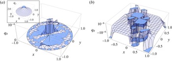
Numerical results from (2.6) and non-dimensional flows normalized with
 ${\it\Omega}Lh$
. (a) The azimuthal flow magnitude is much lower than that of the radial flux. Inset: the radial flow
 $q_{r}$
decays as
 $r^{-1}$
. (b) The angular flow
 $q_{{\it\theta}}$
for a different set of parameters and boundary conditions (see text).

2.1. Circular regime: numerical results
In this section we use the full set of equations (2.6), obtaining numerical results for the bulk, surface velocity fields and cross-sections of the vorticity and pressure. Radial and azimuthal flows are computed numerically, which shows that the angular flow order is much lower than that of the radial flow (see figure 2), and it will be neglected in § 2.2 in a perturbation approach. Numerical stationary solutions of (2.6) in three dimensions are computed using experimental values (Ellegaard et al.
Reference Ellegaard, Hansen, Haaning, Hansen, Marcussen, Bohr, Hansen and Watanabe1999; Martens et al.
Reference Martens, Watanabe and Bohr2012)
 $L=50\times 10^{-3}~\text{m}$
,
 $h=4.1\times 10^{-3}~\text{m}$
,
 $Q=40\times 10^{-6}~\text{m}^{3}~\text{s}^{-1}$
,
 ${\it\nu}=1.1\times 10^{-5}~\text{m}^{2}~\text{s}^{-1}$
,
 ${\it\gamma}=50\times 10^{-3}~\text{N}~\text{m}^{-1}$
,
 ${\it\rho}=1.1\times 10^{3}~\text{kg}~\text{m}^{-3}$
and
 $a=0.01L$
, where
 $a$
is the distance between the free surface and the centre of the jet at the nozzle (see figures 1 and 3
a). Although the Reynolds number is greater than
 $1$
, the inertial lubrication equations contain the information to describe free surface fluid layers. There is a discussion about whether the series in powers of the vertical coordinate converge, which is a mathematical problem in terms of the solutions for the variables
 $\boldsymbol{v}_{0},\ldots ,\boldsymbol{v}_{5}$
and
 ${\it\Pi}_{0}$
,
 ${\it\Pi}_{1}$
,
 ${\it\Pi}_{2}$
. The results obtained from the inertial lubrication equations were validated using different datasets (Rojas et al.
Reference Rojas, Argentina, Cerda and Tirapegui2010; Rojas, Argentina & Tirapegui Reference Rojas, Argentina and Tirapegui2013).
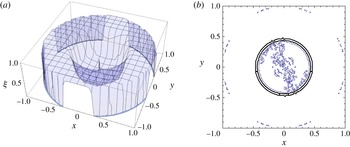
Numerical results from (2.6). (a) Free surface
 ${\it\xi}(r,{\it\theta})$
in the circular regime. (b) The contours of the hydraulic jump condition
 $\partial _{r}^{2}{\it\xi}(r,{\it\theta})=0$
draw one-dimensional curves on the horizontal base; the thick line shows the hydraulic jump position.
Finding the numerical solutions of (2.6) constitutes a boundary-value problem; the solutions are computed using a shooting method with a set of boundary conditions provided at the rim of the plate, different from the conditions proposed by Kasimov (Reference Kasimov2008), where a shallow-water model is obtained from depth-averaged Navier–Stokes equations. The inertial lubrication theory applied to the circular hydraulic jump (Rojas et al.
Reference Rojas, Argentina and Tirapegui2013) is in agreement with Kasimov’s equations in the limit
 ${\it\epsilon}=0$
, where third-order depth gradients are neglected. Numerical solutions of (2.6) are computed from the outer edge to the origin (see figure 3). The fluid height is normalized with the subcritical depth
 $h$
, the horizontal lengths are scaled with
 $L$
, and the radial and azimuthal flows are normalized with the scalar
 ${\it\Omega}Lh$
. The boundary conditions of the free surface at the rim are
 ${\it\xi}(1,{\it\theta})=1$
,
 ${\it\xi}^{(1,0)}(1,{\it\theta})=-0.045409$
,
 ${\it\xi}^{(2,0)}(1,{\it\theta})=0$
(smooth and flat surface at the rim),
 ${\it\xi}^{(0,1)}(r,0)=0$
,
 ${\it\xi}^{(0,1)}(r,2{\rm\pi})=0$
(periodic match at
 ${\it\theta}=0$
). The periodic boundary conditions for the radial flow are
 $q_{r}(1,{\it\theta})=0.5$
(radial flow at the rim),
 $q_{r}(r,0)=1/2r$
,
 $q_{r}(r,2{\rm\pi})=1/2r$
,
 $q_{r}^{(0,1)}(r,0)=0$
,
 $q_{r}^{(0,1)}(r,2{\rm\pi})=0$
(periodic match at
 ${\it\theta}=0$
), where
 $q_{r}={\it\xi}u=1/2r$
is evaluated using the mean radial velocity (see § 2). The periodic conditions for the azimuthal flow are
 $q_{{\it\theta}}(1,{\it\theta})=0$
(no angular flow at the rim),
 $q_{{\it\theta}}^{(1,0)}(1,{\it\theta})=0$
(smooth and flat gradient at
 $r=1$
),
 $q_{{\it\theta}}(r,0)=0$
,
 $q_{{\it\theta}}(r,2{\rm\pi})=0$
,
 $q_{{\it\theta}}^{(0,1)}(r,0)=0$
,
 $q_{{\it\theta}}^{(0,1)}(r,2{\rm\pi})=0$
(periodic match at
 ${\it\theta}=0$
), where
 $f^{(i,j)}(r,{\it\theta})$
indicates the
 $i$
th derivative in
 $r$
and the
 $j$
th derivative with respect to
 ${\it\theta}$
of a function
 $f(r,{\it\theta})$
. The numerical solutions are very sensitive to the selected set of boundary conditions. The conditions on
 $q_{{\it\theta}}$
induce a small drift in the azimuthal direction, negligible in comparison to the radial flow (see figure 2
a, where we use the same conditions except for
 ${\it\xi}^{(1,0)}(1,{\it\theta})=-0.04542$
). In figure 2(b) the modified parameters are the plate radius
 $L=55\times 10^{-3}~\text{m}$
and the subcritical depth
 $h=5.2\times 10^{-3}~\text{m}$
; the boundary conditions remain the same except for the first surface gradient
 ${\it\xi}^{(1,0)}=-0.01359$
. We choose a particular group of boundary conditions focused on
 ${\it\xi}^{(1,0)}(1,{\it\theta})$
; nevertheless different results will be given by distinct ensembles of boundary conditions. Polygonal numerical solutions of (2.6) with a proper set of boundary conditions exist considering, for instance, non-zero azimuthal flow gradients at
 $r=1$
, where two vortices are found in azimuthal cross-sections. The latter has been computed by Passandideh-Fard et al. (Reference Passandideh-Fard, Teymourtash and Khavari2011) using the volume-of-fluid method and will be part of future investigations.
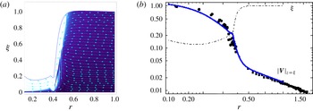
(a) Streamlines of the velocity field (arrows) and free surface (line). The speed magnitude ranges from the lowest (dark) to the fastest (light). (b) Surface velocity (thick line) and profile (dot-dashed line) in log–log scale. Experimental measurements are compared upstream, around the jump (●), and downstream of the jump (▪). Experimental data obtained from Ellegaard et al. (Reference Ellegaard, Hansen, Haaning and Bohr1996). ©The Royal Swedish Academy of Sciences. Reproduced by permission of IOP Publishing. All rights reserved.

We calculate numerical profiles of the fluid–air interface and surface velocity, evaluating the azimuthal coordinate at
 ${\it\theta}=36^{\circ }$
, chosen arbitrarily (see figure 4). Note that, in the centre of the roller at the subsonic region, the speed of the fluid is fast (as in the supersonic region) and decreases radially due to local conservation of angular momentum (see figure 4
a). Experimental data and numerical solutions are normalized with the vessel radius
 $L=70\times 10^{-3}~\text{m}$
. The rest of the dataset remains the same as the one used in figure 2(a). The absolute value of the surface velocity is computed using (2.4) evaluated at
 $z={\it\xi}$
, and normalized with the experimental initial data
 $v_{0}=2.14~\text{m}~\text{s}^{-1}$
(Bohr et al.
Reference Bohr, Ellegaard, Hansen and Haaning1996; Ellegaard et al.
Reference Ellegaard, Hansen, Haaning and Bohr1996). We set the boundary condition for the first surface gradient at the external edge equal to zero, which significantly reduces the oscillations around the jump position (see figure 4
b) in comparison with figure 4 in Rojas et al. (Reference Rojas, Argentina and Tirapegui2013). The boundary conditions at the rim are the same as those used in figure 2(a), with the following changes in the first gradients
 ${\it\xi}^{(1,0)}=0$
and
 ${\it\xi}^{(2,0)}=1.8714389$
. As we increment the system size, the precision required to obtain a numerical solution increases as well, which restricts the possible increase of
 $L$
up to the experimental length (Bohr et al.
Reference Bohr, Ellegaard, Hansen and Haaning1996; Ellegaard et al.
Reference Ellegaard, Hansen, Haaning and Bohr1996). For boundary conditions with more than eight decimals in
 ${\it\xi}^{(2,0)}$
, the form of the solution remains unchanged. By imposing fixed boundary conditions, as the system size is increased, approaching the experimental radius, the numerical profiles of the fluid depth collapse when the fluid surface (
 $z={\it\xi}$
) is in contact with the plate (
 $z=0$
). The surface velocity upstream of the jump is a linear decreasing function in
 $r$
. Around the shock the surface speed scales as
 $(r-c)^{-2/3}$
with
 $c$
a constant related to the position of the jump, and downstream of the jump scales as
 $r^{-1}$
(see figure 4
b).
The magnitude of the vorticity and the streamlines of the velocity field are computed by using the components of
 $\boldsymbol{{\rm\nabla}}\times \boldsymbol{v}$
within the vertical cross-sections
 $z=0.1$
,
 $z=0.5$
and
 $z=0.7$
shown in figure 5. The numerical steps are
 ${\rm\Delta}r=0.05$
and
 ${\rm\Delta}{\it\theta}=0.157$
. The mesh border near to the impinging jet is
 $r=0.01$
with the same parameters and boundary conditions as used in figure 4 except for
 ${\it\xi}^{(2,0)}|_{r=1}=-0.07$
,
 $L=37.9~\text{mm}$
,
 $h=2.77~\text{mm}$
and experimental data given by Bohr et al. (Reference Bohr, Ellegaard, Hansen and Haaning1996) and Ellegaard et al. (Reference Ellegaard, Hansen, Haaning and Bohr1996). The magnitude of the vorticity is normalized with the numerical value
 $2.5\times 10^{5}$
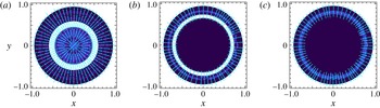
. In the arrowed areas, light rings denote the presence of vorticity regions. In figure 5(a) the light area shows the presence of the recirculation vortex localized at the base of the vessel. In the areas outside of the fluid domain, white sections represent the region
 $r>1$
and dark sections denote
 $z>{\it\xi}$
. In figure 5(b) and 5(c) light rings are produced by the change of the velocity field in that region. Also it could suggest the presence of the surfing roll, which has to be confirmed with angular cross-section computations. For the latter, numerical errors have been observed near the free surface and at the bulk, since the vorticity is strongly non-local, depending on high-order gradients of the surface and the flows. At the numerical scheme, this implies that, close to the fluid–air interface, some values of the vorticity are evaluated outside of the fluid domain (
 $z>{\it\xi}$
), where the flow goes in the opposite direction. This propagates the numerical error into the bulk. These errors can be fixed by defining each gradient near and at the fluid–air boundary by considering that the discrete points of
 $q_{r}$
,
 $q_{{\it\theta}}$
and
 ${\it\xi}$
are zero for
 $z>{\it\xi}$
in the numerical mesh. This will be part of future considerations.
Vertical cross-sections of the vorticity. Streamlines of the velocity field (arrows) and the vorticity magnitude ranging from the lowest (dark) to the highest (light) at
 $z=0.1$
(a),
 $z=0.5$
(b) and
 $z=0.7$
(c). In the arrowed areas, light rings denote the presence of vorticity regions. Areas outside of the mesh domain
 $r>1$
shown in white and
 $z>{\it\xi}$
in dark sections without arrows.

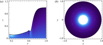
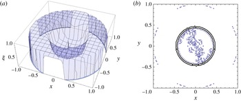
The angular and vertical cross-sections of the magnitude of the pressure in the bulk are calculated by using the third equation in (2.4) (see figure 6). Since the first pressure component
 ${\it\Pi}_{0}$
is related to the velocity by
 $\boldsymbol{v}_{1}=\boldsymbol{{\rm\nabla}}_{\!\bot }{\it\Pi}_{0}$
, we assume that
 $\boldsymbol{v}_{1}$
vanishes asymptotically when
 $r\rightarrow \infty$
, decaying faster than
 $1/r$
, and
 $\boldsymbol{{\rm\nabla}}_{\!\bot }\boldsymbol{\cdot }\boldsymbol{v}_{1}\rightarrow 0$
when
 $r\rightarrow \infty$
faster than
 $1/r^{2}$
. Then, since
 $\boldsymbol{v}_{1}$
is irrotational, the scalar potential
 ${\it\Pi}_{0}$
is computed with
 $$\begin{eqnarray}{\it\Pi}_{0}(r,{\it\theta})=\frac{1}{4{\rm\pi}}\int _{0}^{2{\rm\pi}}\!\int _{0}^{1}r^{\prime }\,\text{d}r^{\prime }\,\text{d}{\it\theta}^{\prime }\,\frac{\boldsymbol{{\rm\nabla}}_{\!\bot }^{\prime }\boldsymbol{\cdot }\boldsymbol{v}_{1}(r^{\prime },{\it\theta}^{\prime })}{(r^{2}+r^{\prime 2}-2rr^{\prime }\cos ({\it\theta}-{\it\theta}^{\prime }))^{1/2}}\end{eqnarray}$$
in polar coordinates (Goldstein, Poole & Safko Reference Goldstein, Poole and Safko1990). Higher pressure components are calculated with
 ${\it\Pi}_{1}=-{\it\epsilon}^{2}\boldsymbol{{\rm\nabla}}_{\!\bot }\boldsymbol{\cdot }\boldsymbol{v}_{0}$
and
 ${\it\Pi}_{2}=-{\it\epsilon}^{2}{\rm\nabla}_{\bot }^{2}{\it\Pi}_{0}$
(Rojas et al.
Reference Rojas, Argentina, Cerda and Tirapegui2010). We plot the pressure at the azimuthal and vertical cross-sections
 ${\it\theta}={\rm\pi}/5$
and
 $z=0.1$
. The magnitude of the pressure difference is normalized with
 $2.5\times 10^{5}$
, and the numerical steps used in figure 6 are
 ${\rm\Delta}r=0.01$
,
 ${\rm\Delta}{\it\theta}=0.1$
and
 ${\rm\Delta}z=0.01$
, the mesh border near to the jet is
 $r=0.01$
with the same boundary conditions and parameters used in figure 5 and experimental data provided by Ellegaard et al. (Reference Ellegaard, Hansen, Haaning, Hansen, Marcussen, Bohr, Hansen and Watanabe1998). In figure 6(a), light regions show areas of high fluid pressure. In figure 6(b) a light ring shows a high-pressure region around the jump position (marked with points). High-pressure areas at
 $r<r_{j}$
are related to the pressure of the impinging jet.
(a) Angular cross-section of the non-dimensional pressure difference at the fluid bulk and free surface profile (continuous line) at
 ${\it\theta}={\rm\pi}/5$
. The pressure magnitude is normalized with the numerical value
 $2.5\times 10^{5}$
for presentation purposes, and it ranges from the lowest (dark) to the highest (light). (b) Vertical cross-section of the pressure magnitude at
 $z=0.1$
. A light ring (marked with points) and centre indicate high-pressure regions. Areas outside of the mesh domain
 $z>{\it\xi}$
and
 $r>1$
shown in white.

2.2. Polygonal states: perturbation theory
In this section we suppose that the angular flow
 $q_{{\it\theta}}(\boldsymbol{x})$
is negligible following previous numerical results (see figure 2) and the approach of Martens et al. (Reference Martens, Watanabe and Bohr2012). Although the azimuthal flow is more important in the polygonal states than in the circular regime, as was shown in detail by Ellegaard et al. (Reference Ellegaard, Hansen, Haaning, Hansen, Marcussen, Bohr, Hansen and Watanabe1998) on the angular flow around polygonal corners, we adopt this ansatz in order to obtain approximate solutions from a perturbation theory performed around the circular state, and thus the horizontal flow is approximated by
 $\boldsymbol{q}(\boldsymbol{x})=(q_{r}(\boldsymbol{x}),0)$
. We utilize the inertial lubrication equations (2.6) standing at a constant radius
 $r_{0}$
from the centre of the jet. The free surface is evaluated at
 $r_{0}$
, then
 ${\it\xi}={\it\xi}({\it\theta})$
. The radial flow is written having angular dependence
 $q_{r}(r,{\it\theta})=C({\it\theta})/2r$
, which implies the circular limit
 $C=1$
(instead of
 $C=0.5$
, see § 2). This solution fulfils the continuity equation (2.6b
) in cylindrical coordinates. The components of vector (2.6a
) provide two differential equations for the variables
 $C({\it\theta})$
and
 ${\it\xi}({\it\theta})$
, equations (2.8) and (2.9),
 $$\begin{eqnarray}\displaystyle & & \displaystyle 7C({\it\theta})[40r^{2}-7{\it\epsilon}^{2}{\it\xi}({\it\theta})^{2}+96{\it\epsilon}^{2}{\it\xi}^{\prime }({\it\theta})^{2}-4{\it\epsilon}^{2}{\it\xi}({\it\theta}){\it\xi}^{\prime \prime }({\it\theta})]-72\mathit{Re}C({\it\theta})^{2}{\it\xi}({\it\theta})\nonumber\\ \displaystyle & & \displaystyle \quad -\,7{\it\epsilon}^{2}{\it\xi}({\it\theta})[38C^{\prime }({\it\theta}){\it\xi}^{\prime }({\it\theta})+7{\it\xi}({\it\theta})C^{\prime \prime }({\it\theta})]=0\end{eqnarray}$$
is the radial coordinate of (2.6a
) where
 ${\it\xi}^{\prime }({\it\theta})=\text{d}{\it\xi}/\text{d}{\it\theta}$
and
 $C^{\prime }({\it\theta})=\text{d}C/\text{d}{\it\theta}$
. By writing the dimensional form of (2.8), the first term is identified with the radial component of the shear force, explained in detail by Martens et al. (Reference Martens, Watanabe and Bohr2012) (see equation (11) therein) and the fifth term is the leading nonlinear contribution in the radial flow. The remaining terms at order
 ${\it\epsilon}^{2}$
are related to viscous and convective nonlinear forces. No hydrostatic terms appear in this equation since we consider
 ${\it\xi}={\it\xi}({\it\theta})$
. Proceeding directly forwards, we solve the azimuthal component of (2.6a
) evaluated at
 $r=r_{0}$
for
 $C({\it\theta})$
,
 $$\begin{eqnarray}C({\it\theta})=\frac{8{\it\xi}^{2}}{9{\it\xi}^{\prime }}\frac{\mathit{Re}}{{\it\epsilon}^{2}Fr}\left[\left(r_{0}^{2}-\frac{{\it\epsilon}^{2}}{\mathit{Bo}}\right){\it\xi}^{\prime }-\frac{{\it\epsilon}^{2}}{\mathit{Bo}}{\it\xi}^{\prime \prime \prime }\right].\end{eqnarray}$$
By writing the dimensional form of (2.9), the first term on the right-hand side is related to the azimuthal component of the hydrostatic force, and the second and third terms are identified with the angular surface tension force (see equations (21) and (42) in Martens et al.
Reference Martens, Watanabe and Bohr2012). The left-hand side of (2.9) is related to the radial component of the shear force. The kinetic and angular shear terms are neglected in this case since we consider zero azimuthal flow or fluid velocity. We replace (2.9) into (2.8) evaluated at
 $r=r_{0}$
and the result is developed in powers of
 ${\it\epsilon}$
until
 $O({\it\epsilon}^{2})$
, which is the highest order used in Rojas et al. (Reference Rojas, Argentina, Cerda and Tirapegui2010). We obtain a third-order ordinary equation that integrated yields
 $$\begin{eqnarray}{\it\xi}^{\prime \prime }+\left(1-\frac{\mathit{Bo}}{{\it\epsilon}^{2}}r_{0}^{2}\right){\it\xi}-\frac{35}{16}\frac{r_{0}^{2}}{{\it\xi}^{2}}\frac{BoFr}{\mathit{Re}^{2}}=C_{0},\end{eqnarray}$$
with
 $C_{0}$
to be determined. The terms in (2.10) are related to the radial shear force, the azimuthal hydrostatic force, the angular surface tension force and nonlinear terms in the radial direction, identified in (2.8) and (2.9), which balance the instability. Exact solutions of (2.10) are written in terms of elliptic integrals, by solving the numerical condition (2.11), which provides functions
 ${\it\xi}({\it\theta})$
in general far from the circular threshold. Equation (2.11) has a trivial solution when
 ${\it\xi}({\it\theta})={\it\xi}_{0}$
is a solution of the polynomial
 $S({\it\xi})=C_{1}-2b_{0}/{\it\xi}+2C_{0}{\it\xi}-a_{0}{\it\xi}^{2}=0$
since
 $(s_{1},s_{2},s_{3})$
are the solutions of
 $S|_{{\it\xi}=s}$
, where
 $a_{0}=(1-r_{0}^{2}\mathit{Bo}/{\it\epsilon}^{2})$
,
 $b_{0}=35r_{0}^{2}BoFr/16\mathit{Re}^{2}$
and
 $$\begin{eqnarray}\left(\frac{2({\it\Gamma}[{\it\phi}_{2},{\it\phi}_{3}]-{\it\Xi}[{\it\phi}_{1},{\it\phi}_{2},{\it\phi}_{3}])}{{\it\theta}+C_{2}}\right)^{2}\frac{s_{1}^{2}({\it\xi}({\it\theta})-s_{1})({\it\xi}({\it\theta})-s_{2})({\it\xi}({\it\theta})-s_{3})}{s_{2}(s_{3}-s_{1}){\it\xi}({\it\theta})}=S({\it\xi}).\end{eqnarray}$$
Here
 ${\it\phi}_{2}=\arcsin \,[\sqrt{(s_{3}-s_{1}){\it\xi}/s_{3}({\it\xi}-s_{1})}]$
,
 ${\it\phi}_{3}=s_{3}(s_{1}-s_{2})/s_{2}(s_{1}-s_{3})$
and
 ${\it\phi}_{1}=s_{3}/(s_{3}-s_{1})$
,
 ${\it\Gamma}[{\it\phi}_{2},{\it\phi}_{3}]$
is the elliptic integral of the first kind, and
 ${\it\Xi}[{\it\phi}_{1},{\it\phi}_{2},{\it\phi}_{3}]$
gives the incomplete elliptic integral of the third kind. The elliptic integrals on the left-hand side of (2.11) converge when
 ${\it\xi}({\it\theta})={\it\xi}_{0}$
is a solution of
 $S$
, which is related to (2.12) and (2.13) through
 $C_{1}=4b_{0}/{\it\xi}_{0}-a_{0}{\it\xi}_{0}^{2}$
(see following text). The latter provides the connection between the first order of the perturbation theory and the exact solutions. In order to solve (2.10) and focus around the circular state, we perform an expansion in a parameter
 ${\it\alpha}$
, which can be set equal to one, and we suppose that the perturbations
 ${\it\xi}_{1}({\it\theta})$
around the fluid depth
 ${\it\xi}_{0}$
are small in comparison to the jump height
 ${\it\xi}_{j}({\it\theta})={\it\xi}_{0}+{\it\alpha}{\it\xi}_{1}({\it\theta})$
. Replacing this into (2.10) at the leading order we have
 $$\begin{eqnarray}C_{0}=\left(1-r_{0}^{2}\frac{\mathit{Bo}}{{\it\epsilon}^{2}}\right){\it\xi}_{0}-\frac{35}{16}\frac{r_{0}^{2}}{{\it\xi}_{0}^{2}}\frac{BoFr}{\mathit{Re}^{2}},\end{eqnarray}$$
or
 $C_{0}=a_{0}{\it\xi}_{0}-b_{0}/{\it\xi}_{0}^{2}$
. We also use approximate solutions since the numerical solutions of (2.11) should be replaced into (2.15) in order to conserve mass flux, which gives more complicated numerical conditions for continuous curves. The order
 ${\it\alpha}$
provides a harmonic oscillator equation for the fluid surface
 ${\it\xi}_{1}^{\prime \prime }+m^{2}{\it\xi}_{1}=0$
, where
 $m$
is the non-dimensional wavenumber of the patterns in the azimuthal coordinate or the number of sides of the solutions in polar coordinates. The notation
 $k$
is restricted to the physical wavenumber, related to the wavelength
 ${\it\lambda}=2{\rm\pi}/k$
. The solutions
 ${\it\xi}_{j}={\it\xi}_{0}+{\it\alpha}(A_{{\it\xi}}/m)\sin m{\it\theta}$
are periodic in
 ${\it\theta}$
, and thus
 ${\it\xi}_{0}$
is equal to the averaged jump depth
 $\bar{{\it\xi}}_{j}=(1/2{\rm\pi})\oint {\it\xi}_{j}({\it\theta})\,\text{d}{\it\theta}$
if and only if
 $m$
is an integer number (the notation
 ${\it\xi}_{0}$
and
 $\bar{{\it\xi}}_{j}$
will be used henceforth indistinctly throughout this paper).
 $A_{{\it\xi}}$
is related to the amplitude of the stationary waves at the surface and
 $$\begin{eqnarray}m=\left(1-{r_{0}}^{2}\frac{\mathit{Bo}}{{\it\epsilon}^{2}}+\frac{35}{8}\frac{{r_{0}}^{2}}{{{\it\xi}_{0}}^{3}}\frac{BoFr}{\mathit{Re}^{2}}\right)^{1/2},\end{eqnarray}$$
or
 $m^{2}=a_{0}+2b_{0}/{\it\xi}_{0}^{3}$
. From (2.12) and (2.13) we obtain
 $C_{0}=m^{2}{\it\xi}_{0}-3b_{0}/{\it\xi}_{0}^{2}$
. Since
 $m$
is a positive number of the order of 1–30 in the polygonal regime, the sum of the terms inside the parentheses of (2.13) has values in the interval
 $[0,10^{3}]$
. The Weber number
 $\mathit{We}={\it\rho}Q^{2}/({\it\gamma}h^{3})=\mathit{Bo}Fr/{\it\epsilon}^{2}$
appears in the second and third terms. The second term
 $r_{0}^{2}\mathit{Bo}/{\it\epsilon}^{2}=r_{0}^{\ast 2}/l_{c}^{2}$
is smaller than
 $1$
(see following text). Equation (2.13) has two limits in terms of the Bond number. The low-surface-tension limit (
 $\mathit{Bo}\rightarrow \infty$
) implies
 ${\it\lambda}\rightarrow 0$
(
 $m\rightarrow \infty$
); in this direction the decrease of surface tension destabilizes the polygonal hydraulic jump to circular type II jumps. In the high-surface-tension limit (
 $\mathit{Bo}\rightarrow 0$
), the increasing of
 ${\it\gamma}$
stabilizes the polygonal jumps towards one-sided polygonal jumps (
 $m=1$
). These limits are in agreement with the findings of Bush & Aristoff (Reference Bush and Aristoff2003), Bush et al. (Reference Bush, Aristoff and Hosoi2006). We suppose that the perturbations
 ${\it\delta}r$
on the azimuthal coordinate around the circular solution at the horizontal plane are of the same order as the stationary waves
 ${\it\xi}_{1}({\it\theta})$
at the free surface
 ${\it\xi}_{0}$
. This assumption was proposed by Martens et al. (Reference Martens, Watanabe and Bohr2012) and is obtained from
 $\partial _{r}^{2}{\it\xi}|_{r=r_{j}}=0$
, which defines the hydraulic jump radius as an inflection point (see figures 3 and 4). Performing a Taylor series expansion of the jump height
 ${\it\xi}_{j}$
around the mean jump radius
 $\bar{r}_{j}=(1/2{\rm\pi}L)\oint r_{j}^{\ast }({\it\theta})\,\text{d}{\it\theta}={\it\lambda}m/2{\rm\pi}L$
(Bush et al.
Reference Bush, Aristoff and Hosoi2006) and neglecting
 $O({\it\delta}r^{2})$
terms, one has
 $$\begin{eqnarray}{\it\xi}(r_{j},{\it\theta})\equiv {\it\xi}_{j}\approx \bar{{\it\xi}}_{j}+c_{1}(r_{j}({\it\theta})-\bar{r}_{j}),\end{eqnarray}$$
where
 $c_{1}$
is the fluid height gradient in the radial direction at the jump position and
 ${\it\delta}r=r_{j}({\it\theta})-\bar{r}_{j}$
. The variations of the free surface
 ${\it\xi}_{1}={\it\xi}_{j}({\it\theta})-\bar{{\it\xi}}_{j}$
around
 $\bar{{\it\xi}}_{j}$
on the azimuthal coordinate are proportional to
 ${\it\delta}r$
, the fluctuations of the hydraulic jump radius around
 $\bar{r}_{j}$
. Equation (2.14) provides a direct connection between
 ${\it\xi}_{j}$
and
 $r_{j}$
. We then write
 $r_{j}({\it\theta})={\it\lambda}m/2{\rm\pi}L+(A_{j}/m)\sin m{\it\theta}$
, where
 $A_{j}=A_{j}^{\ast }/L$
is of the same order as
 ${\it\alpha}A_{{\it\xi}}$
, and provides the orientation
 $r_{j}|_{{\it\theta}=0}=\bar{r}_{j}$
. In the right-hand limit
 $m\rightarrow 0$
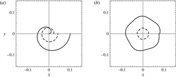
, the solutions are spirals of the form
 $r_{j}=A_{j}{\it\theta}$
(see figure 7
a). For both
 ${\it\xi}_{j}$
and
 $r_{j}$
, their perturbation amplitudes can be more general functions of
 $m^{-{\it\beta}}$
with
 $0<{\it\beta}\neq 1$
. Continuous solutions are obtained in the case
 $m\in \mathbb{N}$
, which are related to the mean radius
 $\bar{r}_{j}^{\ast }={\it\lambda}m/2{\rm\pi}=m/k$
. This condition will be obtained from the perturbation theory when computing the volume conservation at the first order. In the case
 $m\in \mathbb{R}$
, the solutions are discontinuous with a number of sides equal to the integer part of
 $m$
(see figure 7
b). Discontinuous solutions have no physical sense since the hydraulic jump interface must be a continuous curve, i.e. the transition from
 $m=1$
to
 $m=2$
or from
 $m=2$
to
 $m=3$
and so on, is performed in a continuous procedure, without breaking the hydraulic jump interface, as reported in experiments (Ellegaard et al.
Reference Ellegaard, Hansen, Haaning, Hansen, Marcussen, Bohr, Hansen and Watanabe1998; Bush et al.
Reference Bush, Aristoff and Hosoi2006). Irregular or asymmetrical continuous solutions do not appear in this approximation since that is part of a time-dependent transition, which corresponds to a more realistic description of the process where growing defects at the hydraulic jump interface are induced by a change in the height of the outer ring.
(a) Spiral solutions of
 $\bar{r}_{j}$
(continuous line) and
 $q_{r}$
(dashed line) in the interval
 $0<m<1$
for constant flux
 $Q=4\times 10^{-5}~\text{m}^{3}~\text{s}^{-1}$
(see figure 10). (b) Discontinuous five-sided polygon at
 $h=5.22\times 10^{-3}~\text{m}$
. The hydraulic jump radius
 $r_{j}^{\ast }({\it\theta})$
is scaled with the experimental plate radius
 $L=0.18~\text{m}$
and the radial flow
 $q_{r}({\it\theta})$
is reduced with the numerical factor
 $2.\bar{7}\times 10^{-3}$
, computed using (2.13) in addition to (2.17), (2.18) and (2.24b
) (see text). Numerical solutions are plotted using experimental parameters from Ellegaard et al. (Reference Ellegaard, Hansen, Haaning, Hansen, Marcussen, Bohr, Hansen and Watanabe1998). (a)
 $h=5.687~\text{mm}$
; (b)
 $h=5.22~\text{mm}$
.

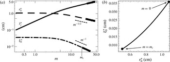
(a) The variable
 $r_{0}^{\ast }$
(dashed line) similar to the wavelength
 ${\it\lambda}$
(see text),
 $\bar{r}_{j}^{\ast }=m{\it\lambda}/2{\rm\pi}$
(continuous line) and
 ${\it\xi}_{0}^{\ast }$
(dot-dashed line) as a function of the number of sides
 $m$
in log–log scale obtained from (2.18) and (2.19). For
 $m>m_{c}$
,
 $(r_{0},{\it\xi}_{0})\in \mathbb{C}$
with a small imaginary part (thick lines). In this interval
 $m$
acquires an imaginary part due to the second and third terms in (2.13). (b) Parametric plot of the solutions
 $r_{0}^{\ast }$
and
 ${\it\xi}_{0}^{\ast }$
obtained from (2.18) and (2.19) varying with
 $m$
. From
 $m=0$
to the critical wavenumber
 $m_{c}$
, the pair
 $(r_{0},{\it\xi}_{0})\in \mathbb{R}$
and decays following (2.18). Numerical solutions of
 $r_{0}^{\ast }$
are in agreement with experimental measurements (Bush et al.
Reference Bush, Aristoff and Hosoi2006).

A marginal instability is defined by the condition
 $m=0$
where the jumps are closed (Craik et al.
Reference Craik, Latham, Fawkes and Gribbon1981) with a mean radius
 $\bar{r}_{j}$
equal to zero. In the interval
 $0<m<1$
the radius of the jump is of the order of the wavelengths. We see in figure 8(a) that
 $r_{0}^{\ast }$
is constant in this interval and decays with
 $m^{-1/2}$
for
 $m>5$
. This suggests that
 ${\it\lambda}$
is similar to
 $2r_{0}^{\ast }$
, which is in agreement with the order of magnitude of the wavelengths measured experimentally (
 ${\it\lambda}\sim 0.7{-}2.0~\text{cm}$
(Bush et al.
Reference Bush, Aristoff and Hosoi2006)), i.e.
 ${\it\lambda}$
has the same dependence on the physical parameters as
 $r_{0}^{\ast }$
. The latter is validated by the connection between (2.13) and Watson’s (Reference Watson1964) theory (see (2.20)–(2.22)). In the interval
 $0<m<1$
the solutions are discontinuous (see figure 7
a) and the mean radius is not well defined. The instability threshold is better described by the condition
 $m=1$
. Here the first continuous solution is reached and the solutions conserve flux (for all integer
 $m$
). In the case
 $m>1$
the instability rises with an increase of the mean radius and a decrease of the wavelengths and the mean jump height (see figure 8
a), as a function of the number of sides determined by the value of
 $m$
. When
 $m\gg 1$
the mean radius of the jump is much greater than the wavelengths, the solutions
 $r_{0}$
and
 ${\it\xi}_{0}$
become complex, and then
 $m^{2}\in \mathbb{C}$
due to the second and third terms of (2.13). Since the number of sides has to be a positive number for polygonal solutions, this provides the cutoff condition for the transition from polygonal to circular type II jumps through the discriminant of the solutions of (2.19) (see following text). Without loss of generality, in the complex regime we consider the solutions of
 ${\it\xi}_{1}^{\prime \prime }+m^{2}{\it\xi}_{1}=0$
to have the harmonic form
 ${\it\xi}_{1}\sim \text{e}^{\text{i}m{\it\theta}}$
, with
 $m={\it\psi}+\text{i}{\it\varphi}$
and
 $({\it\psi},{\it\varphi})\in \mathbb{R}$
. Then the imaginary term is equivalent to the dissipation in a damped harmonic oscillator and the solutions for the jump position are of the form
 $r_{j}({\it\theta})=\bar{r}_{j}+(A_{j}/|m|)\text{e}^{-{\it\varphi}{\it\theta}}\text{e}^{\text{i}{\it\psi}{\it\theta}}$
, which converges to
 $\bar{r}_{j}$
when
 $|m|$
grows (
 ${\it\varphi}$
increases). For
 ${\it\psi}=0$
(
 $m$
completely imaginary), the solutions converge to a circular limit cycle at the real plane of the form
 $r_{j}({\it\theta})=\bar{r}_{j}+(A_{j}/|m|)\text{e}^{-{\it\varphi}{\it\theta}}$
, where
 $\bar{r}_{j}$
corresponds to the radius of circular type II jumps.
The periodic condition for the radial flux (Martens et al. Reference Martens, Watanabe and Bohr2012), related to the fluid mass conservation in the system, indicates that
 $$\begin{eqnarray}\oint \bar{C}({\it\theta})\,\text{d}{\it\theta}=1,\end{eqnarray}$$
with
 $\bar{C}({\it\theta})=C({\it\theta})/2{\rm\pi}$
. The present work is similar to what is performed for the Rayleigh–Plateau instability (Eggers Reference Eggers1997), where a perturbation theory in the vertical coordinate is considered for a fluid column of radius
 $R_{0}$
. In their procedure, the authors obtain a Bessel equation in the radial coordinate. Harmonic solutions proposed for the vertical and temporal components provide a dispersion relation, indicating the dependence of the growth rate
 ${\it\omega}$
on the wavenumber
 $k$
. The main differences with the approach shown in this work are the dynamic effects, not present in the steady polygonal jump. Replacing (2.9) and the solution
 ${\it\xi}_{j}({\it\theta})=\bar{{\it\xi}}_{j}+{\it\alpha}(A_{{\it\xi}}/m)\sin m{\it\theta}$
into (2.15), we expand the result in powers of
 ${\it\alpha}$
. At order
 ${\it\alpha}$
we recover the continuous condition
 $m\in \mathbb{N}$
; this equation is satisfied in order to vanish the azimuthal integral. The leading order yields
 $$\begin{eqnarray}\frac{\mathit{Re}}{Fr}\left(r_{0}^{2}+\frac{{\it\epsilon}^{2}}{\mathit{Bo}}(m^{2}-1)\right)=\frac{9{\it\epsilon}^{2}}{8{\it\xi}_{0}^{2}}.\end{eqnarray}$$
It is important to note that the previous equations (2.13), (2.16) and following equations (2.18), (2.19) are parametric, since the variables
 $r_{0}$
and
 ${\it\xi}_{0}$
are functions of the governing dimensionless groups (Reynolds number, aspect ratio, Froude number and Bond number). We remark that in this work we neglect higher orders in
 ${\it\alpha}$
that provide more information about nonlinear corrections for the patterns of polygonal hydraulic jumps and bumps found recently (Labousse & Bush Reference Labousse and Bush2013). Replacing the harmonic solutions
 ${\it\xi}_{j}({\it\theta})={\it\xi}_{0}+{\it\alpha}(A_{{\it\xi}}/m)\sin m{\it\theta}$
into (2.9) and using (2.16), we find
 $$\begin{eqnarray}C({\it\theta})=1+\frac{2{\it\alpha}A_{{\it\xi}}}{m{\it\xi}_{0}}\sin m{\it\theta}+O({\it\alpha}^{2}),\end{eqnarray}$$
Continuous solutions of the hydraulic jump interface
 $r_{j}({\it\theta})$
(thick line) and radial flux
 $q_{r}({\it\theta})$
(dashed line) in the polygonal regime from
 $h=5.662~\text{mm}~(m=1)$
to
 $h=4.7~\text{mm}$
 $(m=8)$
at constant mass flow density
 $Q=4\times 10^{-5}~\text{m}^{3}~\text{s}^{-1}$
(see figure 10). The hydraulic jump radius
 $r_{j}^{\ast }({\it\theta})$
is scaled with the experimental plate radius
 $L=0.18~\text{m}$
and the radial flow
 $q_{r}({\it\theta})$
is reduced with the numerical factor
 $2.\bar{7}\times 10^{-3}$
, computed using (2.13) in addition to (2.17), (2.18) and (2.24b
) (see text). Numerical solutions are plotted using experimental parameters from Ellegaard et al. (Reference Ellegaard, Hansen, Haaning, Hansen, Marcussen, Bohr, Hansen and Watanabe1998). (a)
 $h=5.662~\text{mm}$
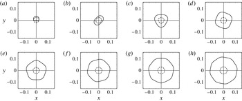
; (b) 5.59 mm; (c) 5.477 mm; (d) 5.336 mm; (e) 5.175 mm; (f) 5.01 mm; (g) 4.851 mm; (h) 4.7 mm.

and thus the radial flux is
 $q_{r}({\it\theta})=(1/2r_{0})(1+(2{\it\alpha}A_{{\it\xi}}/m{\it\xi}_{0})\sin m{\it\theta})$
. The mass conservation condition (2.15) is recovered at order
 ${\it\alpha}$
using (2.17) and neglecting orders
 ${\it\alpha}^{2}$
. We plot the scaled jump radius
 $r_{j}({\it\theta})={\it\lambda}m/2{\rm\pi}L+(A_{j}/m)\sin m{\it\theta}$
and the radial mass flow
 $q_{r}({\it\theta})$
in figures 7 and 9 using (2.13), in addition to (2.18) and (2.24b
), with
 $A_{j}^{\ast }=3\times 10^{-3}~\text{m}$
and
 $2{\it\alpha}A_{{\it\xi}}=9\times 10^{-3}$
. The jump radius
 $r_{j}^{\ast }({\it\theta})$
is normalized with the experimental plate radius
 $L=18~\text{cm}$
(Ellegaard et al.
Reference Ellegaard, Hansen, Haaning, Hansen, Marcussen, Bohr, Hansen and Watanabe1998) and the magnitude of
 $q_{r}({\it\theta})$
is reduced by a factor
 $2.\bar{7}\times 10^{-3}$
for presentation purposes. In the limit
 $m\rightarrow \infty$
, the periodic interface
 $r_{j}({\it\theta})$
converges to the mean radius
 $\bar{r}_{j}$
, which grows with
 $m$
since
 ${\it\lambda}\sim r_{0}^{\ast }$
is nearly constant from
 $m=0$
to
 $m=5$
and decreases slower than
 $m$
for
 $m>5$
(see figure 8
a). As the number of vertices increases, the radial flow solution
 $q_{r}({\it\theta})$
grows (
 $r_{0}\rightarrow 0$
) and its azimuthal dependence decreases (see figure 9). This explains a constant radial flow density in the circular type II case. In this limit the jump height
 ${\it\xi}_{j}({\it\theta})$
converges to the mean jump depth
 $\bar{{\it\xi}}_{j}={\it\xi}_{0}$
and decreases with
 $m$
, which is in agreement with experimental observations (see figure 10). When the number of vertices decreases, the radial flow magnitude decreases since
 $r_{0}$
and
 ${\it\xi}_{0}$
grow,
 $r_{j}({\it\theta})$
reduces in magnitude and its perturbations become more important. In the interval
 $0<m<1$
, the jump radius is not well defined and it has the form of a spiral
 $r_{j}({\it\theta})=A_{j}{\it\theta}$
(see figure 7
a). In this limit, the jump height converges to
 ${\it\xi}_{j}({\it\theta})={\it\xi}_{0}+{\it\alpha}A_{{\it\xi}}{\it\theta}$
, which represents a tilted spiral profile within the radial cross-section
 $r=r_{0}$
. We replace (2.13) into (2.16), which yields the radius
 $r_{0}$
as a function of the fluid depth
 ${\it\xi}_{0}$
:
 $$\begin{eqnarray}r_{0}^{2}={\textstyle \frac{9}{35}}\mathit{Re}{\it\xi}_{0}.\end{eqnarray}$$
The
 $h{-}Q$
phase diagram using numerical solutions from (2.19) and (2.24b
) (continuous lines). One-sided (▫), two-sided (✩), triangles (▵), squares (▪), pentagons (⬠), hexagons (
 $\star$
), heptagons (●) and octagons (○) are shown. Schematic pictures indicate the polygonal curves for the jump radius
 $r_{j}({\it\theta})$
(continuous lines) and the radial flow
 $q_{r}({\it\theta})$
(dashed lines) from
 $m=1$
to
 $m=8$
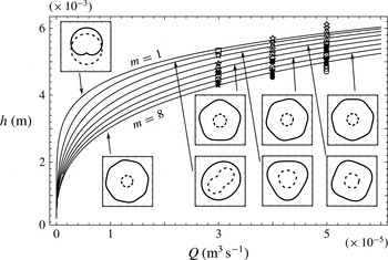
. Experimental data obtained from Ellegaard et al. (Reference Ellegaard, Hansen, Haaning, Hansen, Marcussen, Bohr, Hansen and Watanabe1999). ©IOP Publishing & London Mathematical Society. Reproduced with permission. All rights reserved.

This equation has been found in Rojas et al. (Reference Rojas, Argentina and Tirapegui2013), and resumes the evolution of
 $r_{0}$
and
 ${\it\xi}_{0}$
when
 $m$
varies (see figure 8
b). By replacing (2.18) into (2.13) it is straightforward to review
 $m$
as a function of
 $r_{0}$
. When
 $r_{0}\ll 1$
, the second term in (2.13) decreases, the third term in (2.13) increases and the number of sides of the polygons grows, yielding
 ${\it\lambda}/L\sim (\mathit{Re}\mathit{Bo}Fr)^{1/4}/m^{1/2}$
, which is related to the description of the polygons in the phase diagram (see figure 11). The third term in (2.13) is responsible for the destabilization of circular type II jumps and contains information about
 ${\it\lambda}$
and the characteristic
 ${\it\tau}$
associated with the surfing vortex. In this limit
 $m$
grows and the solutions of (2.19) for
 $r_{0}$
and
 ${\it\xi}_{0}$
are completely real until the critical value
 $m_{c}$
determined by its discriminant,
 $1-1.99(m^{2}-1)^{3}{\it\epsilon}^{4}/\mathit{Bo}^{3}Fr\,\mathit{Re}=0$
, which is the cutoff of
 $r_{0}$
and
 ${\it\xi}_{0}$
in this limit. When
 $r_{0}\gg 1$
, the third term in (2.13) converges to zero (
 ${\sim}r_{0}^{-4}$
) and then
 $m^{2}\rightarrow -\infty$
; nevertheless
 $m^{2}$
is a positive number for circular or polygonal solutions, which yields
 ${\it\lambda}\lesssim h/\mathit{Bo}^{1/2}$
, i.e. the wavelengths are of the same order as the capillary length
 $l_{c}$
when
 $m$
decreases. In this limit the second term is dominant, responsible for the decrease of the number of sides of the polygons until the cutoff
 $m=0$
. Now replacing (2.18) into (2.13) and (2.16) we obtain cubic equations for
 $r_{0}^{2}$
and
 ${\it\xi}_{0}$
related through (2.18):
 $$\begin{eqnarray}\displaystyle {\it\xi}_{0}^{3}+\frac{35{\it\epsilon}^{2}}{9\mathit{Re}\mathit{Bo}}(m^{2}-1){\it\xi}_{0}^{2}-\frac{35{\it\epsilon}^{2}Fr}{8\mathit{Re}^{2}}=0. & & \displaystyle\end{eqnarray}$$
For one-sided polygons (
 $m=1$
) the solutions are
 $r_{0}=(0.744{\it\epsilon}^{2}\mathit{Re}Fr)^{1/6}$
and
 ${\it\xi}_{0}=(4.375{\it\epsilon}^{2}Fr/\mathit{Re}^{2})^{1/3}$
. Equation (2.19) has three solutions for
 ${\it\xi}_{0}$
. In the experimental region of parameters (Ellegaard et al.
Reference Ellegaard, Hansen, Haaning, Hansen, Marcussen, Bohr, Hansen and Watanabe1998), one solution is positive and the rest are negative, and thus the solutions of
 $r_{0}\in \mathbb{R}$
in one case of real
 ${\it\xi}_{0}>0$
due to (2.18). The three solutions of (2.19) are completely real for
 $0<m<m_{c}$
(see figure 8) and become complex at higher values of
 $m$
. A comparative study of (2.19) with the theory of Watson (Reference Watson1964) is performed by considering the case
 $a=0$
(the jet radius, see equation (2.11) in Bush & Aristoff (Reference Bush and Aristoff2003) or (2.20) herein) in the interval downstream of the point
 $r_{v}^{\ast }$
where the boundary layer spans up to the supercritical surface (
 $r^{\ast }>r_{v}^{\ast }$
). We consider the jump height difference
 ${\rm\Delta}H$
to be proportional to the subcritical depth (
 ${\rm\Delta}H={\it\zeta}_{1}h$
) with
 $0<{\it\zeta}_{1}<1$
a non-dimensional variable, which reads
 $$\begin{eqnarray}\frac{\bar{r}_{j}^{\ast 3}}{h^{3}}-0.00835{\it\zeta}_{1}\frac{a}{h}\mathit{Re}^{\prime }We+0.025{\it\zeta}_{1}\frac{\bar{r}_{j}^{\ast 2}}{h^{2}}We+\frac{\bar{r}_{j}^{\ast 3}}{2h^{3}}B_{j}=0,\end{eqnarray}$$
where
 $B_{j}={\it\rho}g\bar{r}_{j}^{\ast }{\rm\Delta}H/{\it\gamma}$
is defined as the jump Bond number. Note that the second term in (2.20) does not depend on
 $a$
since the jet Reynolds number is defined by
 $\mathit{Re}^{\prime }=Q/{\it\nu}a$
. Now replacing (2.18) and
 $m=2{\rm\pi}\bar{r}_{j}^{\ast }/{\it\lambda}$
into (2.19) we obtain an equation independent of the number of sides
 $m$
. We use the change of variables
 $r_{0}^{\ast }={\it\zeta}_{0}\bar{r}_{j}^{\ast {\it\sigma}+1}h^{-{\it\sigma}}$
and
 ${\it\lambda}={\it\zeta}_{2}\bar{r}_{j}^{\ast {\it\eta}+1}h^{-{\it\eta}}$
, where
 ${\it\sigma}$
and
 ${\it\eta}$
are real numbers, and
 ${\it\zeta}_{0},{\it\zeta}_{2}$
are non-dimensional quantities. In the case
 ${\it\sigma}={\it\eta}=-1/2$
,
 $r_{0}^{\ast }$
is similar to the wavelength
 ${\it\lambda}={\it\zeta}_{2}\sqrt{\bar{r}_{j}^{\ast }h}$
and (2.19) yields (2.21). Comparing (2.20) with (2.21) we see similarities in the four terms, where
 ${\it\eta}=-1/2$
is settled in order to match the second terms, which gives
 ${\it\zeta}_{1}\approx 0.007{\it\zeta}_{2}^{2}/{\it\zeta}_{0}^{4}$
. In the case
 ${\it\sigma}=-1/3$
,
 ${\it\eta}=-1/2$
we obtain (2.22) from (2.19). Comparing the third term in (2.22) with the second term in (2.20) we obtain
 ${\it\zeta}_{0}=0.724{\it\zeta}_{1}^{-1/6}$
.
 $$\begin{eqnarray}\displaystyle & \displaystyle \frac{\bar{r}_{j}^{\ast 3}}{h^{3}}-6\times 10^{-5}\frac{{\it\zeta}_{2}^{2}}{{\it\zeta}_{0}^{4}}\frac{a}{h}\mathit{Re}^{\prime }We-\frac{{\it\zeta}_{2}^{2}}{4{\rm\pi}^{2}}\frac{\bar{r}_{j}^{\ast 2}}{h^{2}}+\frac{{\it\zeta}_{0}^{2}{\it\zeta}_{2}^{2}}{4{\rm\pi}^{2}{\it\zeta}_{1}}\frac{\bar{r}_{j}^{\ast 2}}{h^{2}}B_{j}=0, & \displaystyle\end{eqnarray}$$
 $$\begin{eqnarray}\displaystyle & \displaystyle -\frac{1}{2{\it\zeta}_{0}^{2}}\left(\frac{\bar{r}_{j}^{\ast }}{h}\right)^{8/3}+\frac{2{\rm\pi}^{2}}{{\it\zeta}_{0}^{2}{\it\zeta}_{2}^{2}}\left(\frac{\bar{r}_{j}^{\ast }}{h}\right)^{11/3}-\frac{1.2\times 10^{-3}}{{\it\zeta}_{0}^{6}}\frac{a}{h}\mathit{Re}^{\prime }We+\frac{1}{2{\it\zeta}_{1}}\frac{\bar{r}_{j}^{\ast 3}}{h^{3}}B_{j}=0. & \displaystyle\end{eqnarray}$$
 $Q{-}h$
picture: equation
 $Q=m^{1/2}h^{3}/{\it\tau}$
is plotted in continuous lines from
 $m=2$
to
 $m=8$
and
 ${\it\tau}=7.25\times 10^{-3}~\text{s}$
. One-sided (▫), two-sided (✩), triangles (▵), squares (▪), pentagons (⬠), hexagons (
 $\star$
), heptagons (●) and octagons (○) are shown. For
 $m<1$
the hydraulic jump closes; for
 $m\gg 10$
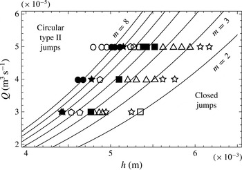
the polygonal solutions converge to a circular jump of type II. Experimental data obtained from Ellegaard et al. (Reference Ellegaard, Hansen, Haaning, Hansen, Marcussen, Bohr, Hansen and Watanabe1999). ©IOP Publishing & London Mathematical Society. Reproduced with permission. All rights reserved.

The last term in (2.22) does not depend on
 ${\it\zeta}_{1}$
. A complete comparison between Watson’s equations and the present work will be developed by determining
 $a$
as a function of the physical variables
 $(\bar{r}_{j}^{\ast },Q,h,\ldots )$
in a future investigation. Equation (2.19) gives information about
 ${\it\xi}_{0}$
as a function of the parameters, which also depends on the number of sides
 $m$
of each polygon. Its solutions are solved numerically using the dataset given by Ellegaard et al. (Reference Ellegaard, Hansen, Haaning, Hansen, Marcussen, Bohr, Hansen and Watanabe1998). In order to describe the experimental measures collected in a phase diagram (figure 10), and since the mean height of the fluid
 $\bar{{\it\xi}}_{j}^{\ast }$
at the jump position differs from the subcritical height
 $h$
, a connection between these variables is necessary. From Rojas et al. (Reference Rojas, Argentina and Tirapegui2013) we obtain information about the critical height
 $h_{c}$
and the outer depth
 $h$
:
 $$\begin{eqnarray}\displaystyle h_{c}=\frac{1}{(4{\rm\pi}^{2})^{1/3}}\frac{Q^{2/3}}{r_{1}^{\ast 2/3}g^{1/3}},\end{eqnarray}$$
 $$\begin{eqnarray}\displaystyle r_{1}^{\ast }=\left(\frac{9}{70{\rm\pi}^{3}}\right)^{1/4}\frac{Q^{3/4}}{{\it\nu}^{1/4}h^{1/2}g^{1/4}}.\end{eqnarray}$$
Equation (2.23b
) is the jump radius as a function of the flux and subcritical height found for hydraulic jumps of type I. This constitutes a first approximation since the polygonal jumps are composed of two vortices within a cross-section
 ${\it\theta}=\text{const}$
. Solving (2.23) we obtain
 $h_{c}$
(2.24a
) as a function of
 $h$
. We suppose that
 $0.17h={\it\xi}_{0}^{1/3}h_{c}$
, which provides
 $0.005<{\it\xi}_{0}$
and
 $0.17<h_{c}/h$
since the critical fluid depth is smaller than the outer height and
 ${\it\xi}_{0}<1$
. The last assumption is related to the physical interpretation of
 ${\it\xi}_{0}$
in terms of
 $h_{c}$
, which will be a subject of consideration in a future investigation. Then multiplying (2.24a
) by
 ${\it\xi}_{0}^{1/3}$
, (2.24b
) is obtained:
 $$\begin{eqnarray}\displaystyle h_{c}=0.733\left(\frac{Q{\it\nu}}{g}\right)^{1/6}h^{1/3},\end{eqnarray}$$
 $$\begin{eqnarray}\displaystyle h=4.3\left(\frac{Q{\it\nu}}{g}\right)^{1/6}\bar{{\it\xi}}_{j}^{\ast 1/3},\end{eqnarray}$$
which relates the dimensional averaged jump depth
 $\bar{{\it\xi}}_{j}^{\ast }={\it\xi}_{0}h$
with the outer height. Equation (2.24b
) is shown in figure 10 by replacing the numerical solutions of
 ${\it\xi}_{0}$
(obtained from (2.19)) into
 $\bar{{\it\xi}}_{j}^{\ast }$
which does not depend on
 $h$
since
 ${\it\xi}_{0}$
depends on
 $h^{-1}$
. This gives more physical insight than the transposed picture (see figure 11), since the outer height depends on the initial fluid current. The equation
 $Q=m^{1/2}h^{3}/{\it\tau}$
describing the phase diagram is derived from dimensional analysis, i.e. it is an equation obtained on the basis that the mass flow density has units
 $[\text{L}]^{3}[\text{T}]^{-1}$
. It is important to remark that the total flux is not correlated to
 $h$
since changes of the outer wall height do not affect the initial fluid current, but it is described as a function of
 $h$
due to its single-valued form. Previous calculations by Martens et al. (Reference Martens, Watanabe and Bohr2012) found
 $Q\sim h^{32/11}$
. We suggest that the characteristic time
 ${\it\tau}$
is related to the flow inside the upper roller, since this feature is shared by circular type II jumps and polygonal states, e.g. the mean time that a fluid particle remains rotating in the surfing vortex, the time that it takes a particle to pass through a polygon corner, or a dissipative time scale related to turbulent eddies, which is of the order of milliseconds (Hondzo Reference Hondzo and Fernando2012).
3. Summary and discussion
We have obtained numerical and approximate solutions of the circular and polygonal hydraulic jumps. The inertial lubrication theory is used to compute numerical solutions of the free surface, radial and angular flows, the bulk and surface velocity fields in addition to azimuthal and vertical cross-sections of the pressure and vorticity magnitudes. The recirculation vortex related to the circular hydraulic jump is computed numerically. Evidence of the second upper roller is found in vorticity calculations and should be confirmed by vertical cross-sections in future investigations. Surface velocity calculations are in agreement with experimental measures, improving previous results. By considering azimuthal symmetries and small perturbations around the circular jump state, we obtain a nonlinear equation that is reduced to a harmonic oscillator for the fluid depth at first order in the polygonal regime. An extended approach considering multiscales in addition to radial and angular dependences of the free surface will be conducted in a future research work. We identify the forces driving and resisting the instability, which are: the radial shear force, the azimuthal surface tension and the hydrostatic azimuthal force, in addition to a nonlinear term in the radial coordinate. The thresholds of the instability are defined at closed jumps (
 $m=0$
) for discontinuous curves and at one-sided polygonal jumps (
 $m=1$
) for continuous solutions conserving fluid mass density. Exact solutions of (2.10) are related to elliptic integrals, which should give results for the wavelengths of the polygons as a function of the surface tension. This will be part of a future consideration along with a Hamiltonian approach describing
 ${\it\xi}$
and
 ${\it\xi}^{\prime }$
in
 ${\it\theta}$
.
The solutions of the leading and first order of a hierarchy of equations explain the transition from type II circular jumps to polygonal and closed jumps when the outer height
 $h$
is increased, and describe the reduction of the mean jump radius or the radial flow magnitude and the growth of their wavelengths as the number of sides decreases at the jump interface. Higher-order equations are neglected, but nevertheless are related to the description of diverse patterns found by Labousse & Bush (Reference Labousse and Bush2013), which could explain, for instance, different polygonal shapes with the same number of vertices. The wavelengths of the polygons are found to be similar to the variable
 $r_{0}^{\ast }$
, which is supported by comparison with experimental measurements and a comparative study with Watson’s (Reference Watson1964) theory. A continuation of this work will provide answers for the physical meaning of
 ${\it\xi}_{0}^{\ast }$
(related to
 $h_{c}$
), and the variables
 ${\it\zeta}_{0}$
,
 ${\it\zeta}_{1}$
and
 ${\it\zeta}_{2}$
that might be improved by considering the case
 $a\neq 0$
. In the limit
 $m\rightarrow 0$
, spiral solutions are found for the jump radius and the radial flow, which is related to the closing process of the polygons when the external fluid height is increased. When
 $m\gg 1$
, a cutoff for the height and radius of the jump is found when the solutions
 $r_{0}$
and
 ${\it\xi}_{0}$
become complex at the critical non-dimensional wavenumber
 $m_{c}$
. The solutions in this interval converge to the mean results similarly as a damped harmonic oscillator in the azimuthal coordinate, explaining the transition mechanism at the frontier between the polygonal and circular type II jumps. In this limit, the wavelength of the polygons is found to be a function of the Reynolds, Bond and Froude numbers. This is related to the
 $h{-}Q$
phase diagram, which is described by an approximation obtained from the perturbation theory and a power law given by dimensional analysis. In a Cartesian geometry, (2.6) can be applied to the hydraulic jump problem at an inclined plane. By considering a non-inertial rotating reference frame, the present work can be extended to the study of rotating polygons (Vatistas Reference Vatistas1990; Jansson et al.
Reference Jansson, Haspang, Jensen, Hersen and Bohr2006; Bergmann et al.
Reference Bergmann, Tophøj, Homan, Hersen, Andersen and Bohr2011; Tophøj et al.
Reference Tophøj, Mougel, Bohr and Fabre2013) found recently.
Acknowledgements
The authors acknowledge T. Bohr for providing permissions and useful experimental measures. E.T. thanks project Fondecyt 1120329. N.R. acknowledges the support of CONICYT PAI/Academia 79112030.