1. Introduction
The Asia-Pacific region has played a pivotal role in the global economy’s tumultuous recovery since COVID-19. According to data from the International Monetary Fund, China and India are jointly projected to contribute approximately half of the world’s economic growth in 2024. Since 1979, China has pursued a policy of opening up to foreign trade and investment, coupled with a series of free-market reforms. As a result, it has emerged as one of the world’s fastest-growing economies, with a real annual gross domestic product (GDP) growth averaging 9.5% through 2018, as reported by the World Bank. In Figure 1a, we illustrate China’s GDP and GDP growth rate from 2000–2022. Over the past two decades, the nation’s economy has expanded significantly, achieving its highest growth rate of 14.2% in 2007. However, the 2008 financial crisis and the COVID-19 pandemic have subsequently slowed down China’s growth. Between these events, China experienced steady growth, albeit at a decreasing speed. Although China’s growth slowed after 2007, it has maintained an average rate of 7% until 2022.
China’s GDP and Number of Manufacturing Firms.Notes: The GDP and the number of legal entities in manufacturing data are sourced from the Bureau of Statistics of China, while the GDP shares are collected from the World Development Indicators.

The rapid growth of China’s economy finds its roots in manufacturing, making the country the world’s primary manufacturing superpower. According to data from the OECD TiVA database in 2023, China’s gross production (total sales of manufacturers) constitutes 35% of global production, surpassing the sum of the USA and Japan, which account for 12% and 6%, respectively. Figure 1b illustrates a notable increase of over 2.6 times in the number of legal entities in manufacturing over the past two decades. China’s manufacturing industries contribute approximately 30% to GDP, with an average annual growth rate of 13% from 2004 to 2020. This robust economic development has attracted significant attention from researchers and economists, prompting examinations of China’s manufacturing productivity changes and their sources (see, for example, Bosworth and Collins, Reference Bosworth and Collins2008; Brandt and Zhu, Reference Brandt and Zhu2010; Perkins and Rawski, Reference Perkins and Rawski2008; Brandt et al., Reference Brandt, Van Biesebroeck and Zhang2012; Song et al., Reference Song, Storesletten and Zilibotti2011; Zhu, Reference Zhu2012). Despite this interest, accurately identifying the sources of China’s manufacturing output and productivity growth requires consistent estimation of production technologies, adjustments for evolving economic conditions, and accommodation of firm and industry heterogeneity. These factors are often overlooked in previous decomposition exercises. Therefore, building on recent developments in the literature on production function identification and decomposition methods, this paper aims to examine the sources of output and productivity growth in China’s listed manufacturing companies, taking into account these crucial factors.
This study focuses on analyzing China’s growth sources between 2000 and 2022, categorizing the two decades into four distinct phases. The first phase, spanning 2000–2007, marked a few features, such as the continuation of economic reforms and the transformation from a planned economy to a market-oriented one, China’s accession to the World Trade Organization (WTO), and its integration into the world economic system. During this period, the country actively participated in economic globalization, promoted industrial structural improvements, and enhanced the competitiveness of its industries (Xie, Reference Xie2023). China experienced thriving economic growth during this period. The second phase, spanning 2008 to 2012, was characterized by efforts to overcome challenges arising from the global financial crisis of 2008. China faced a shrinking international market demand and a slowdown in domestic economic growth. After 2010, economic growth further decelerated due to a slowdown in export growth, reduced foreign direct investment inflows, and increased production costs. These challenges led to the closure, relocation, or transformation of many manufacturing enterprises. The third phase, from 2013–2017, centered on the goal of transforming into a strong industrial country, promoting high-quality development, and building a new modern industrial system. During this period, China implemented a higher level and a wider range of opening-up policies to safeguard and promote global free trade. However, in 2018, China’s economy faced cooling pressures from faltering domestic demand and the impact of the US-China trade war, resulting in the lowest growth level in nearly three decades. The post-2019 era has been influenced by the coronavirus pandemic. China implemented a “dynamic clearance strategy” and a series of stabilizing policies to restrict the dissemination of the COVID virus since the reopening of Wuhan in early April 2020. Additionally, efforts were made to promote high-quality development and effectively coordinate epidemic control and economic development. So, the last phase, from 2018–2022, included recent challenges faced by China.
In manufacturing data, it’s common to observe significant variations among firms in terms of production and technology, and Chinese producers are no exception. However, traditional decomposition studies often make the simplifying assumption that all firms share the same production technology, typically characterized by a Cobb–Douglas production function with constant input elasticities. Moreover, these studies typically apply decomposition only at the mean of the output distribution, overlooking substantial heterogeneity among firms. This approach may be overly restrictive and inconsistent with the actual data. In our paper, we address these limitations by introducing flexibility and mitigating mis-specification errors from two perspectives. First, we allow for firms’ production functions to be unknown smooth functions and estimate them in a nonparametric manner. Second, we extend our decomposition analysis to both the mean and various quartiles of the output distribution. This is crucial because, as evidenced by the asymmetric distribution of firms’ output, the traditional mean decomposition fails to capture the representativeness of firms of different sizes.
From the technical perspective, the challenge in implementing output quantile decomposition arises from the fact that coefficients in regular quantile regressions lack direct interpretation as the marginal effects of independent variables on the unconditional quantile of the dependent variable. A noteworthy contribution of this paper lies in the decomposition of firms’ output growth into the contributions of inputs and productivity at various quantiles. To achieve this, we employ the recentered influence function (RIF) regression method introduced by Firpo et al. (Reference Firpo, Fortin and Lemieux2009). The RIF method possesses a desirable property where the expectation of any distributional statistic’s RIF equals the statistic itself. Leveraging this property, we assume that the conditional expectation of the RIF of output quantiles is a flexible function of a firm’s inputs and productivity. Applying the law of iterated expectations, we can then decompose the changes in the unconditional quantiles of a firm’s output into its inputs and productivity.
Given the significant attention focused on estimating the productivity of Chinese firms (see, for example, Song et al., Reference Song, Storesletten and Zilibotti2011; Brandt et al., Reference Brandt, Van Biesebroeck and Zhang2012; Jin et al., Reference Jin, Zhao and Kumbhakar2019; Malikov et al., Reference Malikov, Zhao and Kumbhakar2020; Hou et al., Reference Hou, Jin and Kumbhakar2020), coupled with frequent market-oriented economic reforms and changes in firm ownership, we extend our analysis to decompose the market-share-weighted industry aggregate productivity growth by considering different ownership types. In doing so, we contribute an application and extension of the productivity decomposition method initially developed by Olley and Pakes (Reference Olley and Pakes1996) and its dynamic version proposed by Melitz and Polanec (Reference Melitz and Polanec2015).
To decompose the sources of output and productivity growth, our first step involves identifying and estimating a firm’s production function and productivity. The consistent estimation of these factors has been the subject of recent extensive study, with a primary challenge being the latent productivity, which is unobserved by econometricians but correlated with the firm’s endogenous input usage. In this paper, we adopt the approach presented by Gandhi et al. (Reference Gandhi, Navarro and Rivers2020), utilizing the first-order condition in a firm’s short-run profit maximization problem and the proxy variable method to estimate the firm’s production function and productivity. To account for the heterogeneity in firms’ production technology, we employ a flexible nonparametric production function.
The data utilized in this paper is derived from a comprehensive firm-level panel obtained from the China Stock Market Accounting Research (CSMAR) database, which focuses on China’s Finance and Economy. CSMAR, developed by Shenzhen CSMAR Data Technology Co., Ltd., aligns with international professional standards while catering to China’s unique features. To have a full picture of China’s manufacturing sector, another widely used database is the Chinese Industrial Enterprise Database, which include all state-owned and all non-state-owned firms with sales above 5 million CNY, approximately 0.6 million USD. However, this database includes high-quality data only from 1998–2007. To explore China’s economic growth trends in more recent years, we use the CSMAR database in this paper. Although CSMAR focuses on large listed companies, it effectively reflects China’s economic development over the past two decades. We find that the expansion of China’s manufacturing sector largely follows the country’s economic growth. Before the 2008 financial crisis, both increased materials usage and firm productivity progress contribute significantly to output growth. However, after 2008, productivity advancement slows down for median-sized and large firms. There is a notable shift in the role of productivity as a driver of output growth, especially for the median and large firms at the second and third quartiles of the output distribution. Specifically, while productivity growth was a significant contributor to output growth from 2000–2007, it turns into negative values in more recent years. For the industry aggregate productivity growth, we find the productivity improvement of state firms is the key driver before the 2008 financial crisis. However, in recent years, only private firms still exhibits noticeable productivity advancement. Over the entire sample period, there is no clear evidence of output reallocation efficiency improvement in China’s manufacturing sector.
The findings of this study suggest the need for nuanced policy interventions to sustain and enhance China’s economic growth, particularly in the manufacturing sector. Given the observed slowdown in productivity advancement among median-sized and large firms post-2008, policymakers should focus on creating an environment that fosters innovation and productivity improvements within these firms. This could include targeted incentives for technological development and increased support for research and development. Furthermore, the significant productivity gains from private firms indicate that these enterprises could be key drivers of future growth. Therefore, policymakers should design policies that encourage the expansion and competitiveness of private firms, such as reducing barriers to entry, enhancing access to capital, and promoting fair competition. Additionally, the lack of evidence for output reallocation efficiency suggests potential inefficiencies in resource allocation. Reforms aimed at improving market mechanisms and promoting a more efficient reallocation of resources toward more productive firms are crucial. Finally, the comprehensive insights provided by the CSMAR database highlight the need for differentiated strategies that account for the varying opportunities and challenges faced by firms of different sizes and ownership structures. Policymakers should leverage this data to craft informed, evidence-based economic policies.
To summarize, the paper makes several key contributions. First, it investigates the factors behind the expansion of China’s industrial output by examining the extent to which total factor productivity (TFP) and input growth explain the growth. It accounts for the heterogeneity in production technology and sources of growth across firms of different sizes. The paper decomposes the output growth of listed manufacturing firms into input deepening and productivity boost, considering both the mean and quartiles of the output distribution. Second, the paper applies dynamic industry aggregate productivity decomposition methods to assess the heterogeneous contributions of firms with different ownerships. It connects to the extensive literature examining state and foreign firms and their contributions to China’s economy. Third, and more importantly, this paper provides evidence on China’s manufacturing sector over the most recent two decades, encompassing the 2008 financial crisis, the economic growth slowdown, further economic transitions, trade conflicts with the USA, and the COVID-19 pandemic. It shows how Chinese firms of varying sizes and types have responded to these challenges.
The remainder of this paper is organized as follows: Section 2 is a brief review of previous studies on production function estimation and decomposition methods. Section 3 outlines the methodologies employed to decompose output and productivity growth. Section 4 provides details about the data used. Results are presented in Section 5, and Section 6 concludes the paper. Additional data description, estimation details, and robustness check from a value-added production function are provided in the appendix.
2. Literature review
In this section, we provide a brief literature review on the production function estimation and decomposition methods. For more detailed reviews on these two topics, see Ackerberg et al. (Reference Ackerberg, Caves and Frazer2015) and Huang et al. (Reference Huang, Zhao and Kumbhakar2022).
One challenge that received tremendous attention in empirical applications recovering production functions is the simultaneity issue—firms’ latent productivity is correlated with input usage, and one would obtain inconsistent estimation if the unobserved productivity is uncontrolled. Fundamentally, this is an endogeneity issue generated by unobservables. In the literature, one approach is to use panel data models with fixed effects, assuming a time-invariant productivity shock,
 $\omega _i$
, to address the endogeneity problem (e.g., Hoch, Reference Hoch1955, Reference Hoch1962; Mundlak, Reference Mundlak1961). Unfortunately, one common issue with this approach is the unreasonably low estimates of capital elasticities and returns to scale (Griliches and Mairesse, Reference Griliches and Mairesse1998). More recent works, such as Arellano and Bover (Reference Arellano and Bover1995) and Blundell and Bond (Reference Blundell and Bond2000), have generalized this approach to accommodate more sophisticated error structures. An alternative approach to estimate production functions leverages information from firms’ profit maximization or cost minimization behavior or their corresponding first-order conditions with respect to inputs, as seen in Griliches and Ringstad (Reference Griliches and Ringstad1971) and Hall (Reference Hall1988). This approach has been developed in various studies. Notably, Olley and Pakes (Reference Olley and Pakes1996) propose a structural framework to identify production functions. They assume that firm’s heterogeneity/productivity is not only individual-specific but also time-varying. Their identification strategy relies on a discrete-time model of dynamically optimizing firms, in which they express firms’ latent productivity as the inverse function of investment. Levinsohn and Petrin (Reference Levinsohn and Petrin2003) suggest inverting the input demand function for an intermediate material input and applies a proxy variable method similar to Olley and Pakes (Reference Olley and Pakes1996). Ackerberg et al. (Reference Ackerberg, Caves and Frazer2015) discuss possible functional dependence problems in prior works and propose a new estimator for value-added production functions. Different from previous studies, Gandhi et al. (Reference Gandhi, Navarro and Rivers2020) explicitly use firms’ first-order condition as an estimation equation and propose a nonparametric estimator for gross production functions. We apply the methodology outlined by Gandhi et al. (Reference Gandhi, Navarro and Rivers2020) in our analysis to estimate firm production functions and productivity for its flexibility.
To examine the sources of output growth, the conventional growth accounting approach often assumes a restrictive log-linear Cobb–Douglas production function, and the contribution parameters of production factors to output growth are measured by the shares of these factors in the aggregate output under the assumption of constant returns to scale. For example, in the context of China, Wang and Yao (Reference Wang and Yao2003) construct a measure of China’s human capital stock over 1952–1999 and employ it in the standard growth accounting exercise. They find a significant role played by human capital accumulation to growth and welfare. Bosworth and Collins (Reference Bosworth and Collins2008) employ a similar approach to compare sources of economic growth in China and India between 1978 and 2004, and they show that the TFP growth is the most important driver for the growth in China’s manufacturing sector. The conventional growth accounting approach ignore the heterogeneity of production technologies among firms and across industries, and it can be considered as a mean decomposition method, which shows average contributions of production factors to output growth. The output growth decomposition method used in this paper is more flexible in terms of allowing for heterogeneous production technologies and providing evidence beyond the output mean.
To decompose aggregate productivity, a recent influential work is from Olley and Pakes (Reference Olley and Pakes1996), who focus on the within-industry reallocation of market share toward more productive firms, thereby enhancing aggregate productivity. Several related decomposition methods have been developed in the literature to analyze the sources of aggregate productivity growth from either the firm dynamics or resource allocation perspectives. For example, Baily et al. (Reference Baily, Hulten, Campbell, Bresnahan and Caves1992) provides an accounting framework that tracks productivity changes over time by comparing firms’ productivity and market share at two points in time. Foster et al. (Reference Foster, Haltiwanger and Krizan2001) includes a cross-term that captures the interaction between productivity and changes in market shares, providing a richer view of reallocation dynamics than Olley and Pakes (Reference Olley and Pakes1996). Griliches and Regev (Reference Griliches and Regev1995) focuses on the contributions of continuing firms and net entry to productivity growth in a simpler static decomposition compared to Olley and Pakes (Reference Olley and Pakes1996). Melitz and Polanec (Reference Melitz and Polanec2015) propose an extension of the Olley and Pakes (Reference Olley and Pakes1996) productivity decomposition that accounts for the contributions of surviving, entering, and exiting firms to aggregate productivity changes. A similar study to ours in terms of understanding the recent industry productivity performance is from Coyle et al. (Reference Coyle, McHale, Bournakis and Mei2024). They focus on the UK economy from 2008–2019. From estimating a revenue production function, they find an overall fall in TFP levels in manufacturing and a striking decline of between 13% and 18% in the level of within-firm manufacturing TFP. Comparing with previous studies, the productivity decomposition method in this paper is tailored to China’s business environment, emphasizing the roles of firms’ ownership, which can potentially change the ways of business operation.
3. Decomposition methods
In this section, we elaborate on our decomposition methods aimed at identifying the sources of output and productivity growth for Chinese listed manufacturing companies. We decompose output growth into input accumulation and productivity change. To accommodate firm heterogeneity, we follow Huang et al. (Reference Huang, Zhao and Kumbhakar2022) by considering decomposition methods at both the mean and quantiles of the output distribution. Additionally, drawing from Olley and Pakes (Reference Olley and Pakes1996), we decompose industry aggregate productivity into sources of productivity progress and reallocation efficiency: productivity progress measures the unweighted average firm productivity changes, while reallocation efficiency measures the increase in output achieved by reallocating production from low-productive firms to high-productive ones. Given the significance of state-owned enterprises and foreign investment in the development of the Chinese economy, we also examine productivity progress within, and allocation efficiency among, foreign, state, and private domestic firms.
3.1. Output growth decomposition
We consider the following gross production function for firm
 $i$
at time
 $t$
, which converts multiple production inputs into a scalar output (
 $Y$
):
 \begin{equation} Y_{it}=G(K_{it},L_{it},M_{it})e^{\omega _{it}+\eta _{it}}, \end{equation}
where
 $K_{it}$
,
 $L_{it}$
, and
 $M_{it}$
represent capital, labor, and materials inputs, respectively. This production function has two stochastic error terms:
 $\omega _{it}$
, representing the firm’s persistent Hicks-neutral productivity, and
 $\eta _{it}$
, a random productivity shock or measurement errors in output, with
 $E(\eta _{it}) = 0$
. Such a straightforward setup has been widely used in the literature of production and productivity analysis (see, for example, De Loecker, Reference De Loecker2011; Doraszelski and Jaumandreu, Reference Doraszelski and Jaumandreu2013; Asker et al., Reference Asker, Collard-Wexler and De Loecker2014; Brandt et al., Reference Brandt, Van Biesebroeck, Wang and Zhang2017; Malikov et al., Reference Malikov, Zhao and Kumbhakar2020; Gandhi et al., Reference Gandhi, Navarro and Rivers2020; Huang et al., Reference Huang, Zhao and Kumbhakar2022).
To accommodate the heterogeneous production technologies among firms, we refrain from imposing parametric functional forms on
 $G({\cdot})$
. Instead, we require only that the unknown function
 $G({\cdot})$
is smooth, and then estimate it nonparametrically following the procedure proposed by Gandhi et al. (Reference Gandhi, Navarro and Rivers2020). Identifying gross production functions such as Equation (3.1) is generally non-trivial. The main challenge arises from the simultaneity issue, where firms’ input choices
 $(K_{it}, L_{it}, M_{it})$
are determined based on the unobserved productivity
 $\omega _{it}$
. Without appropriately controlling for their correlation, the estimated production function will be biased, akin to estimates in a typical omitted variable situation.
Recent literature conventionally relies on structural assumptions regarding firm production and profit maximization or cost minimization behavior to construct multiple-step estimation procedures. For example, see Olley and Pakes (Reference Olley and Pakes1996), Petrin and Levinsohn (Reference Petrin and Levinsohn2012), Ackerberg et al. (Reference Ackerberg, Caves and Frazer2015), and Gandhi et al. (Reference Gandhi, Navarro and Rivers2020). We choose to utilize the method proposed by Gandhi et al. (Reference Gandhi, Navarro and Rivers2020) due to its flexibility in handling a nonparametric production function and its popularity in applied studies of production and productivity analysis. The basic idea of their estimator is to first partially identify the production function from the first-order condition of a flexible input (in this case
 $M_{it}$
) in the firm’s profit maximization problem. Then, they use the fundamental theorem of calculus and a Markov assumption on the productivity term
 $\omega _{it}$
to fully identify the function
 $G({\cdot})$
.
The details of the estimation steps are provided in our appendix. Since these details do not pertain to the contribution of the current study, we do not elaborate on the estimation further. In the subsequent discussion of the decomposition methods, we treat
 $G({\cdot})$
and
 $\omega _{it}$
as if they were “observed.”
3.1.1. Mean decomposition
The decomposition of output at its mean based on an estimated production function has a long history in economic analysis. It dates back to as early as the pioneer work of Solow (Reference Solow1957), who describe “an elementary way of segregating variations in output per head due to technical change from those due to changes in the availability of capital per head.” Here, we distinguish ourselves from most previous studies that assume log-linear Cobb–Douglas production technologies in terms of decomposition methodologies by considering a flexible relationship between firms’ output and inputs, and therefore allowing for greater heterogeneity.
Taking the logarithm of Equation (3.1), we have
 \begin{equation} y_{it}=g(k_{it},l_{it},m_{it}) + \omega _{it}+\eta _{it}, \end{equation}
where
 $g({\cdot}) \equiv \ln G({\cdot})$
, and throughout the paper, we use the lower-case letters to represent the log values of the corresponding upper-case counterparts. Based on the log production function (3.2), firm
 $i$
’s expected output growth from period 1 to 2 can be written as:
 \begin{align} \triangle ^\mu _O \equiv & E\left [y_{i2}\right ]-E[y_{i1}] \nonumber \\ = & \underbrace{E \left [g(k_{i2},l_{i2},m_{i2})\right ]-E[g(k_{i1},l_{i2},m_{i2})]}_{\triangle ^\mu _k} + \underbrace{E[g(k_{i1},l_{i2},m_{i2})]-E[g(k_{i1},l_{i1},m_{i2})]}_{\triangle ^\mu _l} \nonumber \\ & +\underbrace{E[g(k_{i1},l_{i1},m_{i2})]-E[g(k_{i1},l_{i1},m_{i1})]}_{\triangle ^\mu _m}+\underbrace{E[\omega _{i2}]-E[\omega _{i1}]}_{\triangle ^\mu _\omega }. \end{align}
We use
 $\triangle ^\mu _O$
to represent the growth of output at its mean. We decompose it into contributions of capital, labor, materials, and productivity, denoted by
 $\triangle ^\mu _k$
,
 $\triangle ^\mu _l$
,
 $\triangle ^\mu _m$
, and
 $\triangle ^\mu _\omega$
, respectively.
To implement the above decomposition for Chinese listed manufacturing firms, we need to replace the mathematical expectation operator with its sample counterpart. During the calculation, we require firm
 $i$
to be observable in both periods 1 and 2. In other words, the decomposition in (3.3) is conducted based on the same set of firms in periods 1 and 2.Footnote
1
In Equation (3.3), to isolate the contribution of each input to the output growth, we begin by examine the change in capital from periods 1 to 2, followed by the changes in labor and materials. Consider
 $\triangle _k^{\mu }$
as an example. It relies not only on the differences in capital values between the two periods but also on the values of labor and materials in period 2. Similarly,
 $\triangle _l^{\mu }$
and
 $\triangle _m^{\mu }$
face analogous issues. Consequently, the values of
 $\triangle ^\mu _k$
,
 $\triangle ^\mu _l$
, and
 $\triangle ^\mu _m$
are path-dependent. This means their magnitudes depend on the specific order of {
 $k$
,
 $l$
,
 $m$
} in which the decomposition is conducted. Hence, in the results section, we present the averages of all decomposition outcomes obtained from all possible permutations (3!), ensuring that the reported results are robust and path-independent.
3.1.2. Quantile decomposition
While we employ a nonparametric production function described in Equation (3.1) to account for the diverse production technologies across firms, the decomposition outlined in Equation (3.3) only centers on the mean output of firms. However, it is essential to recognize that the entire output distribution exhibits considerable variation. Firms, varying in production scale, may diverse significantly in terms of output growth and productivity innovation. To delve into this further, we next introduce our quantile decomposition method.
Conducting a quantile decomposition of output growth is more challenging than the mean decomposition, since a direct application of the conventional (conditional) quantile regression will not offer us the desired estimates that show the contributions of production inputs and productivity to the unconditional output quantiles, which show changes of all firms. The challenge here is that the law of iterated expectations does not apply in the case of conditional quantiles. See Fortin et al. (Reference Fortin, Lemieux and Firpo2011) for more discussion. To overcome this hurdle, we follow the approach of Firpo et al. (Reference Firpo, Fortin and Lemieux2009) and Huang et al. (Reference Huang, Zhao and Kumbhakar2022) by employing the RIF method.
Specifically, for the
 $\tau$
-th quantile of output
 $y_{it}$
,
 $q_\tau$
, we can construct its RIF as:
 \begin{equation} \text{RIF}(y_{it};\, q_\tau ) = q_\tau + \frac{\tau -1\{y_{it}\leq q_\tau \}}{f_{y_{it}}(q_\tau )}, \end{equation}
where
 $f_{y_{it}}(q_\tau )$
represents the density function of
 $y_{it}$
evaluated at
 $q_{\tau }$
, and
 $1\{\cdot \}$
is an indicator function. For any given dataset,
 $q_{\tau }$
and
 $f_{y_{it}}(q_\tau )$
can be estimated empirically. Specifically, we can estimate
 $q_\tau$
by minimizing the check function (Koenker and Bassett, Reference Koenker and Bassett1978):
 $\hat{q}_\tau =\arg \min _q\sum _{i,t} (\tau -1\{y_{it}-q \leq 0\})\cdot (y_{it}-q)$
. We can estimate
 $f_{y_{it}}({\cdot})$
using the local constant kernel density estimator, that is,
 $\hat{f}_{y_{it}}({q}_\tau )=\frac{1}{NT \cdot h} \sum _{i,t} \mathcal{K}_{y_{it}}\left (\frac{y_{it}-{q}_\tau }{h}\right )$
, where
 $\mathcal{K}_{y_{it}}\left (\cdot \right )$
is a kernel function, for which we use the
 $2$
nd order Gaussian kernel, and
 $h$
is the bandwidth, which can be selected by the leave-one-out cross validation method. Then,
 $\text{RIF}(y_{it}; q_\tau )$
can be considered as “observed.” Next, we estimate the expectation of
 $\text{RIF}(y_{it}; q_\tau )$
conditional on firms’ production inputs and productivity to identify their contributions to the RIF of the
 $\tau$
-th quantile of output:
 \begin{equation} E\left [\text{RIF}(y_{it};\, q_\tau ) \ | \ k_{it}, l_{it}, m_{it}, \omega _{it}\right ] = f(k_{it}, l_{it}, m_{it}, \omega _{it}). \end{equation}
Note that Equation (3.5) is a regression model, with the dependent variable of
 $\text{RIF}(y_{it}; q_\tau )$
and independent variables of
 $k_{it}$
,
 $l_{it}$
,
 $m_{it}$
, and
 $\omega _{it}$
. Similar to the estimation of the production function (3.1), we assume no specific functional forms of
 $f({\cdot})$
and estimate it using the series estimator based on the second-order polynomial basis.
One desirable property of the RIF is that, for any distributional statistic of a random variable
 $y$
denoted by
 $v(F_{y})$
, the expectation of its RIF is equal to itself. Applying this property and the law of iterated expectation to our situation, we have
 $q_\tau =E\left [ E\left [\text{RIF}(y_{it}; q_\tau ) \ | \ k_{it}, l_{it}, m_{it}, \omega _{it} \right ] \right ]$
. Then, we can decompose output growth at quantiles. Specifically, for any
 $\tau$
and two periods, denoted by 1 and 2, we have
 \begin{align} & \bigtriangleup ^{q_\tau }_O \equiv \ q_{\tau 2} - q_{\tau 1} \nonumber \\ = & \underbrace{E \left [f(k_{i2},l_{i2},m_{i2},\omega _{i2})\right ]-E[f(k_{i1},l_{i2},m_{i2},\omega _{i2})]}_{\triangle ^{q_{\tau }}_k} + \underbrace{E[f(k_{i1},l_{i2},m_{i2},\omega _{i2})]-E[f(k_{i1},l_{i1},m_{i2},\omega _{i2})]}_{\triangle ^{q_{\tau }}_l} \nonumber \\ & +\underbrace{E[f(k_{i1},l_{i1},m_{i2},\omega _{i2})]-E[f(k_{i1},l_{i1},m_{i1},\omega _{i2})]}_{\triangle ^{q_{\tau }}_m}+\underbrace{E[f(k_{i1},l_{i1},m_{i1},\omega _{i2})]-E[f(k_{i1},l_{i1},m_{i1},\omega _{i1})]}_{\triangle ^{q_{\tau }}_{\omega }}, \end{align}
where we use
 $q_{\tau 1}$
and
 $q_{\tau 2}$
to denote the
 $\tau$
-th quantile of output in periods 1 and 2, respectively. In Equation (3.6), we decompose the growth of output at quantile
 $\tau$
into contributions coming from capital (
 $\triangle ^{q_{\tau }}_k$
), labor (
 $\triangle ^{q_{\tau }}_l$
), materials (
 $\triangle ^{q_{\tau }}_m$
), and productivity (
 $\triangle ^{q_{\tau }}_{\omega }$
).
Similar to the mean decomposition, there are several noteworthy points to consider when implementing the quantile decomposition outlined above. First, in our latter application of Chinese listed manufacturing companies, we replace the mathematical expectation operator with its finite sample counterpart. This entails working with a balanced panel across periods 1 and 2.Footnote
2
Second, the order of
 $(k,l,m,\omega )$
in which the decomposition is conducted matters for the estimated contribution of inputs and productivity to output growth. In total, there are twenty-four (4!) different possible permutations for each output quantile. To eliminate the path dependence nature of (3.6), we compute and report the average of decomposition results from all permutations for each quantile in the subsequent section.
3.2. Productivity growth decomposition
“Productivity isn’t everything, but in the long-run it is almost everything. A country’s ability to improve its standard of living over time depends almost entirely on its ability to raise its output per worker.” said Paul Krugman in his book The Age of Diminished Expectations. To gain a more comprehensive understanding of the expansion of China’s manufacturing sector through the lens of listed companies, we extend our analysis by decomposing the industry aggregate productivity growth into two potential sources: productivity progress and reallocation efficiency.
3.2.1. Static O-P decomposition
The pioneer work of Olley and Pakes (Reference Olley and Pakes1996) proposes a decomposition method that breaks the industry aggregate productivity, which is defined as the output market-share-weighted average of individual productivity, into two components: an unweighted mean of firm productivity and a covariance between firm’s output share and productivity. The first component captures the technological/productivity progress within firms (when we have a balanced panel across two periods), and the second component measures whether the entire industry produces more outputs by moving resources from less productive companies to more productive ones. The specific formula of this decomposition is
 \begin{equation} \Phi _t \equiv \sum _{i}s_{it}\omega _{it}=\bar{\omega }_t + \sum _{i}(s_{it}-\bar{s_t})(\omega _{it}-\bar{\omega }_t), \end{equation}
where
 $\Phi _t$
is the industry aggregate productivity,
 $s_{it}$
is the output market share, defined as
 $s_{it}={Y_{it}}/{\sum _{i=1}^{N_t} Y_{it}}$
, where
 $N_t$
is the number of companies in period
 $t$
, and for any variable
 $a$
,
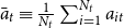 $\bar a_t \equiv \frac{1}{N_t} \sum _{i=1}^{N_t} a_{it}$
.
In our subsequent empirical application involving Chinese listed manufacturing companies, we implement the aforementioned decomposition. Our objective is to identify the primary contributor to industry productivity and assess its variation across our sample period, which is characterized by varying economic growth rates.
3.2.2. Dynamic ownership decomposition
The conventional Olley and Pakes (Reference Olley and Pakes1996) decomposition is commonly regarded as a static approach, as it does not account for changes in productivity and reallocation efficiency over time or across different groups of firms. Building on the work of Melitz and Polanec (Reference Melitz and Polanec2015), we further extend our analysis to include a dynamic decomposition of industry aggregate productivity growth among various categories of listed companies.
Since the late 1970s, China has undergone significant market-oriented economic reforms and shifts in ownership structures. State-owned enterprises have encountered intensified market competition and pressure, prompting many, particularly small and less profitable ones, to undergo substantial restructuring and downsizing. This process often involves bankruptcy, sales and auctions, as well as mergers and acquisitions. Simultaneously, China has opened up to the rest of the world and transformed into one of the largest foreign investment destinations.
In acknowledge of the dynamic ownership changes and the pivotal roles played by state and foreign firms in China’s economic growth, we categorize all listed firms into three groups: foreign, state, and private. A firm is classified as a foreign firm (
 $F=1$
) in a given year if it holds foreign equity (
 $FHMT\gt 0$
), including shares from Hong Kong, Macao, and Taiwan. A firm is categorized as a state firm (
 $ST=1$
) if it does not possess foreign equity but holds state equity (
 $SOE\gt 0$
). All other firms are classified as domestic private firms (
 $P=1$
).
For any two consecutive periods 1 and 2, we can write industry aggregate productivity as:
 \begin{align*} &\Phi _1 = s_{F_1} \Phi _{F_1} + s_{ST_1} \Phi _{ST_1} + s_{P_1} \Phi _{P_1}, \\ &\Phi _2 = s_{F_2} \Phi _{F_2} + s_{ST_2} \Phi _{ST_2} + s_{P_2} \Phi _{P_2}, \end{align*}
where the subscripts
 $F$
,
 $ST$
, and
 $P$
stand for foreign, state, and private firms, respectively;
 $s_{G}$
with
 $G \in \{F, ST, P\}$
is the total market share for firms in group
 $G$
, that is,
 $s_{G_t} \equiv \sum _{i\in G} s_{it}$
;
 $\Phi _G$
is the market-share-weighted, group-specific aggregate productivity, that is,
 $\Phi _{G_t} \equiv \sum _{i\in G} \frac{s_{it}}{s_{G_t}} \omega _{it}$
. Then, we can define the industry aggregate productivity growth as the difference between
 $\Phi _2$
and
 $\Phi _1$
:
 \begin{equation*} \bigtriangleup \Phi \equiv \Phi _2 - \Phi _1 = \sum _{G \in \{F, ST, P\}} \Big ((s_{G_2}-s_{G_1})\Phi _{G_1} + s_{G_2} (\Phi _{G_2}-\Phi _{G_1})\Big ). \end{equation*}
Moving from the first equality to the second, we use the property that
 $s_{G_2} \Phi _{G_2} - s_{G_1} \Phi _{G_1}=(s_{G_2}-s_{G_1})\Phi _{G_1} + s_{G_2} (\Phi _{G_2}-\Phi _{G_1})$
. To better interpret the above decomposition, we can use the aggregate productivity in the first period as a reference group and compare the group-specific productivity against it. To do that, note that
 $s_{F_t}+s_{ST_t}+s_{P_t}=1$
, for
 $t=$
1 or 2, which suggests
 $\sum _{G \in \{F, ST, P\}} s_{G_2}\Phi _1 = \sum _{G \in \{F, ST, P\}} s_{G_1}\Phi _1$
. Thus, we can further write the above equation as
 \begin{equation} \bigtriangleup \Phi = \sum _{G \in \{F, ST, P\}} \Big (\underbrace{(s_{G_2}-s_{G_1})(\Phi _{G_1}-\Phi _1)}_{\text{Reallocation Efficiency}} + \underbrace{s_{G_2} (\Phi _{G_2}-\Phi _{G_1})}_{\text{Productivity Progress}}\Big ). \end{equation}
In Equation (3.8),
 $s_{G_2} (\Phi _{G_2} - \Phi _{G_1})$
captures the technological/productivity progress within each type of firm, and
 $(s_{G_2}-s_{G_1})(\Phi _{G_1}-\Phi _1)$
measures the ownership reallocation efficiency. For instance, if state firms are in general becoming more productive over time due to economic reforms, we will find
 $\Phi _{ST_2} \gt \Phi _{ST_1}$
. Therefore, the productivity progress term
 $s_{ST_2} (\Phi _{ST_2} - \Phi _{ST_1})$
will be positive. Additionally, if state firms are, on average, less productive than the industry average, that is,
 $\Phi _{ST_1} \lt \Phi _1$
, an efficient way to reallocate production among different types of firms suggest a decrease in state firms’ market share, which means
 $s_{ST_2} \lt s_{ST_1}$
. Consequently, the reallocation efficiency measure
 $(s_{ST_2}-s_{ST_1})(\Phi _{ST_1}-\Phi _1)$
will be positive, indicating an improvement in efficiency.
In our following empirical application, we apply the dynamic decomposition outlined above to study Chinese listed manufacturing companies, aiming at identifying the importance of state firm reforms, foreign investment, and the resilience of private enterprises in driving China’s growth over the past two decades.
4. Data
The data we use in this study are obtained from the CSMAR database, which is a comprehensive database focused on Chinese financial and economic data.Footnote 3 CSMAR includes sections/sub-databases of stock market data, financial statements of listed companies, corporate governance information, economic indicators, industry-specific data, and research tools. It is widely utilized by researchers, analysts, and investors for empirical research and analysis related to the Chinese stock market and accounting practices (e.g., Wang, Reference Wang2010; Li et al., Reference Li, Lu, Mittoo and Zhang2015; Du et al., Reference Du, Boateng and Newton2016; Ma et al., Reference Ma, Sun, Waisman and Zhu2016; He and Kyaw, Reference He and Kyaw2018; Rathnayake et al., Reference Rathnayake, Kassi, Louembe, Sun and Ding2019). While there are three types of stocks in the Chinese stock market: A, B, and H shares, in this study, we focus on A-share manufacturing firms for their dominant role.Footnote 4
We primarily utilize data from two (sub-)databases of CSMAR. Specifically, we make use of the Financial Statement Database, which comprises the balance sheet, income statement, and statement of cash flow (indirect method) tables. This database reports items on a quarterly basis; however, for our study, observations are aggregated on an annual basis. Following CSMAR’s guidelines, we use end-of-year observations in the annual reports. Additionally, we utilize the Corporate Governance Database, which contains general information on corporate governance, capital structure, and basic company profile tables. To adjust monetary values for inflation, we gather price indices from the China Economic Research (CER) Series Database.
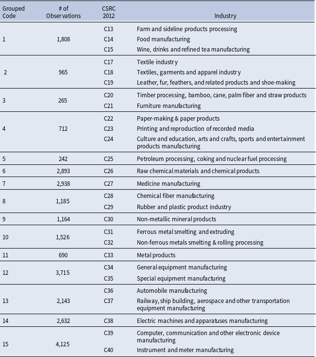
Adhering to the guidelines outlined in the Industry Classification of Listed Companies issued by the China Securities Regulatory Commission (CSRC) in 2012, we retain firms falling within categories C13-C40 (excluding C16), encompassing manufacturing industries. Subsequently, to accommodate the relatively small number of observations in some industries, we categorize the 27 industries into 15 groups based on their characteristics. Table 1 lists all manufacturing industries included in this study, their categorization, and the corresponding number of observations.
Industry classification and group

We define firms’ output (
 $Y$
) as their operating revenue and measure their capital (
 $K$
) and labor (
 $L$
) inputs using net fixed assets and the total number of employees, respectively. We construct the measure of the materials input (
 $M$
) using its related components.Footnote
5
We deflate all monetary values using price indices from the CER database in 1990 constant prices: output is deflated using the ex-factory price index of industrial products; capital is deflated using the industrial GDP deflator; materials are deflated using the purchasing price index of raw materials, fuel, and power. Additionally, we define two ownership variables: foreign shares (
 $FHMT$
) measured as the percentage of stocks held by investors from abroad (including H shares, B shares, and other shares) and state shares (
 $SOE$
) measured as the percentage of stocks held by the state. A firm is classified as a foreign-invested firm (
 $F=1$
) in a given year if the firm owns foreign equity (
 $FHMT\gt 0$
), including equity from Hong Kong, Macao, and Taiwan. A firm is classified as a state-invested firm (
 $ST=1$
) in a given year if the firm does not own foreign equity but owns state equity (
 $SOE\gt 0$
). The rest of the firms are referred to as (domestic) private firms (
 $P=1$
). We exclude observations with missing values for the above key variables. Additionally, when estimating a production function, following the approach outlined by Guariglia et al. (Reference Guariglia, Liu and Song2011), Malikov et al. (Reference Malikov, Zhao and Kumbhakar2020), and Huang et al. (Reference Huang, Zhao and Kumbhakar2022), we drop the top and bottom 0.5th percentiles of production variables, including observations with negative values, to mitigate the impact of extreme values on estimation.
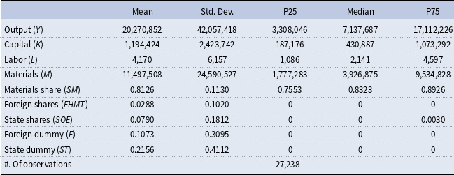
Our final sample includes 3,088 A-share listed firms over the period from 2000 to 2022. The summary statistics, including the mean, standard deviation, 25th percentile, median, and 75th percentile of the key variables, are presented in Table 2. For all production variables, the means exceed the corresponding medians, indicating right-skewed distributions. Compared with manufacturing firms in the widely used Chinese Industrial Enterprises Database (see the data summary by Huang et al., Reference Huang, Zhao and Kumbhakar2022), the listed firms are much larger on average—they produce more output, use more capital and materials, and hire more employees.Footnote 6 Across all firms, 10.75% are foreign-invested firms, 21.56% are state-invested firms, and the remainder are private firms.
Summary statistics

Notes: The values of output (
 $Y$
), capital stock (
 $K$
), and materials (
 $M$
) are measured in hundreds of real RMB, and labor (
 $L$
) is measured by the total number of employees. “Materials Share (
 $SM$
)” is the ratio of materials to the output value. “Foregin Shares (
 $FHMT$
)” is the percentage of stocks held by investors from abroad; “SOE” measures the percentage of stocks held by the state. “F” is a dummy variable which equals 1 if a firm is classified as a foreign-invested firm; 0 otherwise. “SOE” is a dummy variable which equals 1 if a firm is classified as a state-invested firm; 0 otherwise. The table reports the mean (Mean), standard deviation (Std. Dev.), 25th percentile (P25), median (Median), and 75th percentile (P75) of the key variables.
5. Empirical results
In this section, we present our output and productivity decomposition results for Chinese listed manufacturing firms, derived from the methods outlined in the preceding section. Given the substantial heterogeneity across industries in our sample, we apply our estimation steps and decomposition analysis separately to each of the 15 industry groups listed in Table 1. As the group-specific results contain a plethora of information which may overwhelm readers and obscure key takeaway lessons, we report their average across all industry groups in the subsequent tables.Footnote 7
Output mean decomposition

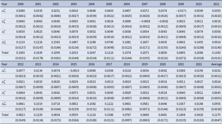
Notes: Row “Total” refers to the average output growth from the preceding year, which is equal to the sum of the contributions from productivity (
 $\Delta _\omega ^\mu$
), capital (
 $\Delta _k^\mu$
), labor (
 $\Delta _l^\mu$
), and materials (
 $\Delta _m^\mu$
). Column “Average” shows the overall averages between 2000 and 2022. Standard errors of cross-industry mean estimates are reported in parentheses.
5.1. Output growth decomposition
As shown in Sections 3.1.1 and 3.1.2, the output growth can be broken down into contributions from capital, labor, materials growth, and neutral productivity advance. Due to the flexible functional forms applied for firms’ production function (3.1) and the conditional expectation of RIF at different output quantiles (3.5), our output decomposition results are path-dependent—the order of
 $(k, l, m)$
or
 $(k, l, m, \omega )$
in which the decomposition is executed matters. There are six (3!) distinct permutations for the mean decomposition and twenty-four (4!) different permutations for each of the quantile decomposition. In this section, we calculate and report their average to make the results path-independent.
5.1.1. Mean decomposition
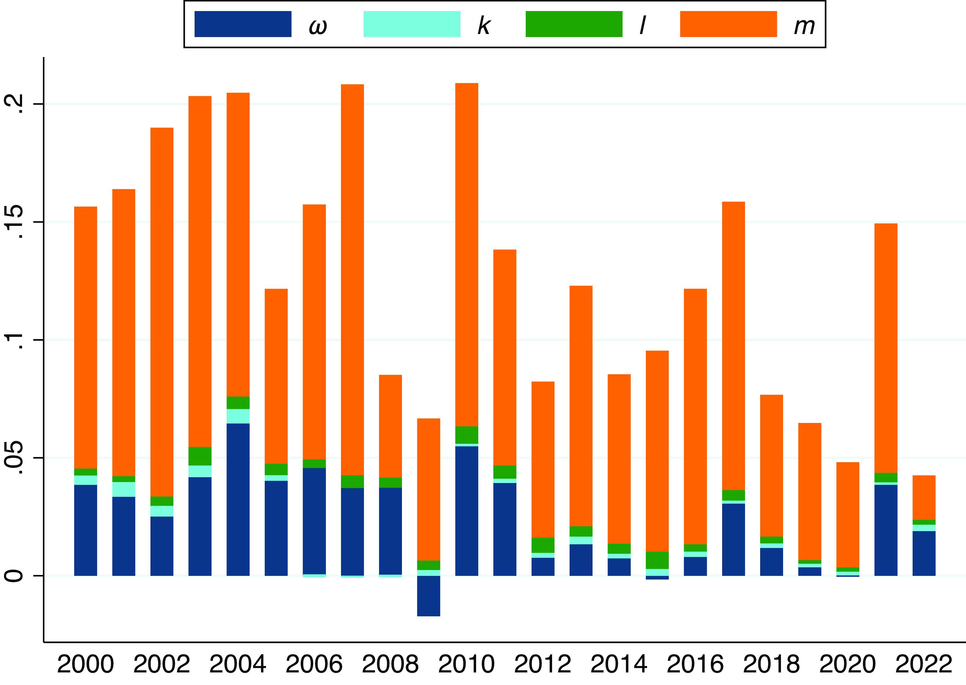
Table 3 displays the mean output decomposition results over the years in our sample period, while Figure 2 visualizes the contributions of production factors and productivity to the output growth. Based on the differences in economic growth rates and development strategies in China from 2000–2022, we partition our entire sample period into four sub-periods. The first period spans from 2000–2007, characterized by rapid GDP growth and swift industrial expansion. During this period, Chinese listed manufacturing companies on average experience significant growth, with annual growth rates ranging from 12.15–20.74% with the mean of 17.56%. The production technologies and firm productivity of Chinese manufacturing firms in this period have been well examined by previous studies that use the comprehensive Chinese Industrial Enterprises Database (see, e.g., Brandt et al., Reference Brandt, Van Biesebroeck and Zhang2012; Malikov et al., Reference Malikov, Zhao and Kumbhakar2020; Huang et al., Reference Huang, Zhao and Kumbhakar2022; Malikov and Zhao, Reference Malikov and Zhao2023). A closely related study among them is from Huang et al. (Reference Huang, Zhao and Kumbhakar2022), who conduct similar output decomposition analysis for all medium- and large-sized manufacturing firms during this period. They find that the average annual output growth rate of Chinese manufacturing firms from 1999–2007 is 9.27%, and the contributions to output growth coming from firm productivity progress and capital, labor, materials input deepening are 3.18%, 0.38%, 0.05%, and 5.67%, respectively. As discussed in the data section, our listed companies are much larger compared with the firms examined by Huang et al. (Reference Huang, Zhao and Kumbhakar2022). Our firms grow much faster in this period. As to the contributions to the output growth, productivity progress contributes 2.52% to 6.47% with the mean of 4.09%, materials input deepening contributes 7.39% to 16.57% with the mean of 12.68%, and the contributions from other inputs are negligible.
Output mean decomposition for listed manufacturing firms. Notes: Notations
 $\omega$
,
 $k$
,
 $l$
, and
 $m$
refer to the contributions from productivity, capital, labor, and materials to firms’ output growth, respectively.

The second period, from 2008–2012, encompasses the global economic crisis and its subsequent recovery. During this timeframe, there is a marked slowdown in output growth, with significant contractions in 2008 and 2009, where growth rates fall to 8.5% and 4.95%, respectively, in these two years. This is followed by a strong rebound in 2010, with output growth surging to 20.88%, before stabilizing at more moderate levels of 13.83% in 2011 and 8.23% in 2012. In 2009, firm productivity temporarily has a negative impact on output growth, likely due to adjustments made in response to the post-crisis economic situation. In the following year, the productivity growth surges to 5.49%, but then gradually declines over time. In the entire period, the average output growth rate is 11.28%, with contributions from firm productivity, capital, labor, and materials inputs being 2.44%, 0.15%, 0.56%, and 8.13%, respectively.
The third period spans from 2013 to 2017, immediately following the 18th National Congress of the Chinese Communist Party. During this five-year period, China transitions from a phase of rapid economic growth to a more moderate one. The economic objective also shifts from “growth at all costs” to “high-quality development.” Consequently, the average annual industrial output growth of Chinese listed companies varies between 8.53% to 15.85%, with an average of 11.56%, slower than the first period and approximately at the same rate as the second period. Upon examining the sources of the output growth, we find that the contribution from firm productivity progress is close to zero, except for year 2017, in which the average productivity growth is 3.05%. In other years, the output growth is almost entirely driven by materials growth. Given that productivity innovations are often considered as the fundamental drivers of long-term economic growth, the absence of evidence for significant productivity progress during this period may raise concerns, particularly for list manufacturing companies.
The last period covers from 2018–2022. It is characterized by a further slowdown in industrial output growth, driven by the compounded effects of the US and China trade conflict and China’s stringent COVID policies. Specifically, the average output growth rate of Chinese listed manufacturing firms ranges from 4.26–7.67%, with an exception in year 2021, which shows a growth rate of 14.93%. During the entire period, the average output growth rate is 7.63%. The contribution of productivity to output growth is relatively higher in the years 2018, 2021, and 2022, at 1.18%, 3.86%, and 1.90%, respectively. The increase in materials usage remains the key source of output growth.
The last column of Table 3 displays the average decomposition over the entire sample period. The dynamic changes of the Chinese economy in the past 23 years have been hidden by the average numbers in this column. Therefore, in the subsequent analysis, similar to Table 3 and Figure 2, we also provide phase-specific interpretations of our empirical results.
In sum, while China’s manufacturing sector has shown resilience in the face of various economic shocks, the diminishing role of productivity growth, especially in the more recent years, signals potential vulnerabilities. To sustain long-term economic growth, it will be crucial for China to reinvigorate productivity through innovation and more efficient resource allocation. The findings suggest that future policy efforts should focus on fostering a competitive environment that supports productivity improvements.
5.1.2. Quantile decomposition
While the above mean decomposition provides valuable insights for firms whose size aligns with the industry average in terms of production and input usage, it may offer less information for large or small firms positioned at the tails of the output distribution. Given the vast number and significant heterogeneity of Chinese manufacturing firms, we are prompted to conduct a quantile decomposition, as outlined in Section 3.1.2, to achieve a more comprehensive understanding of China’s industry expansion.
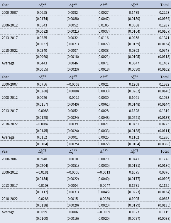
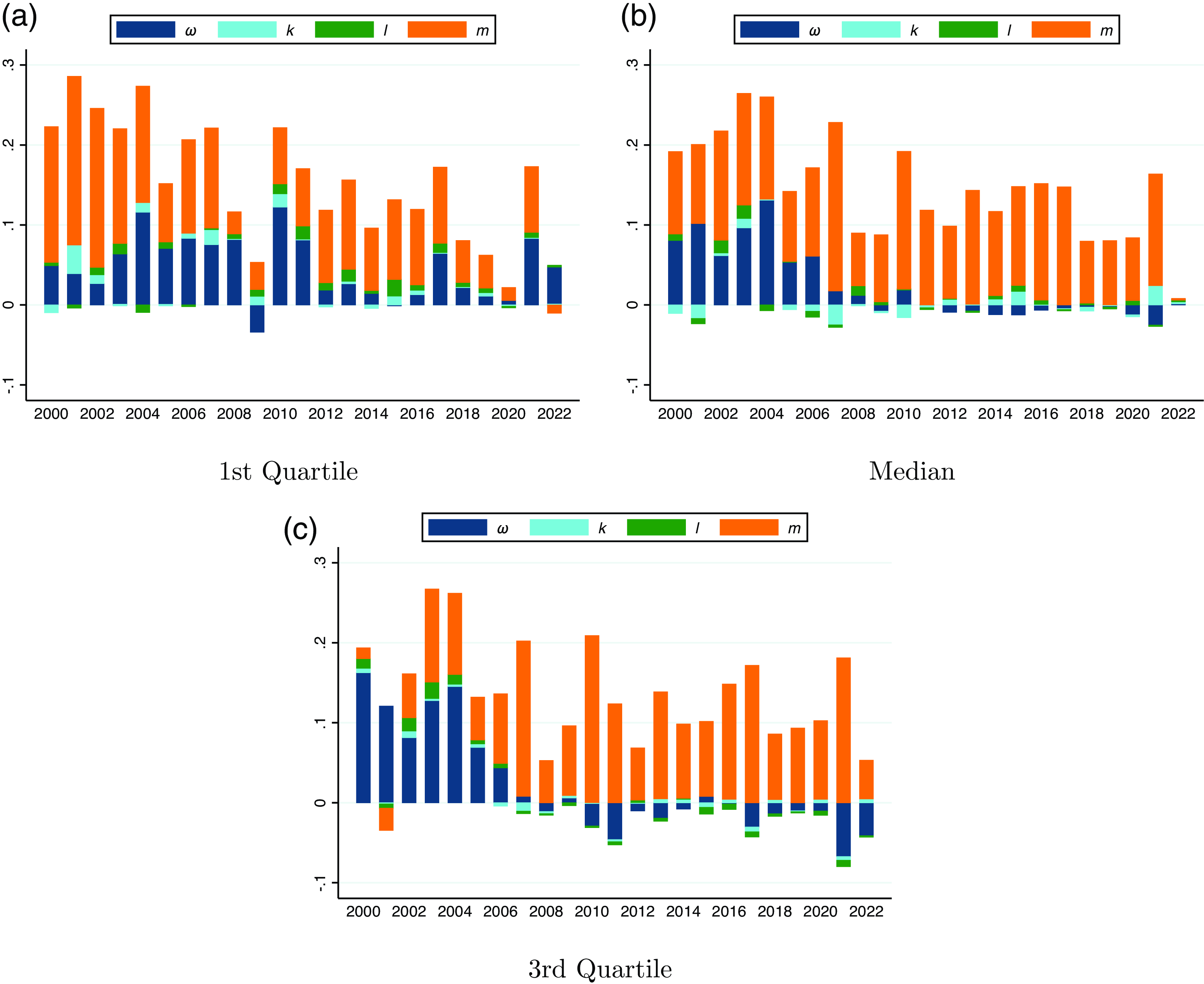
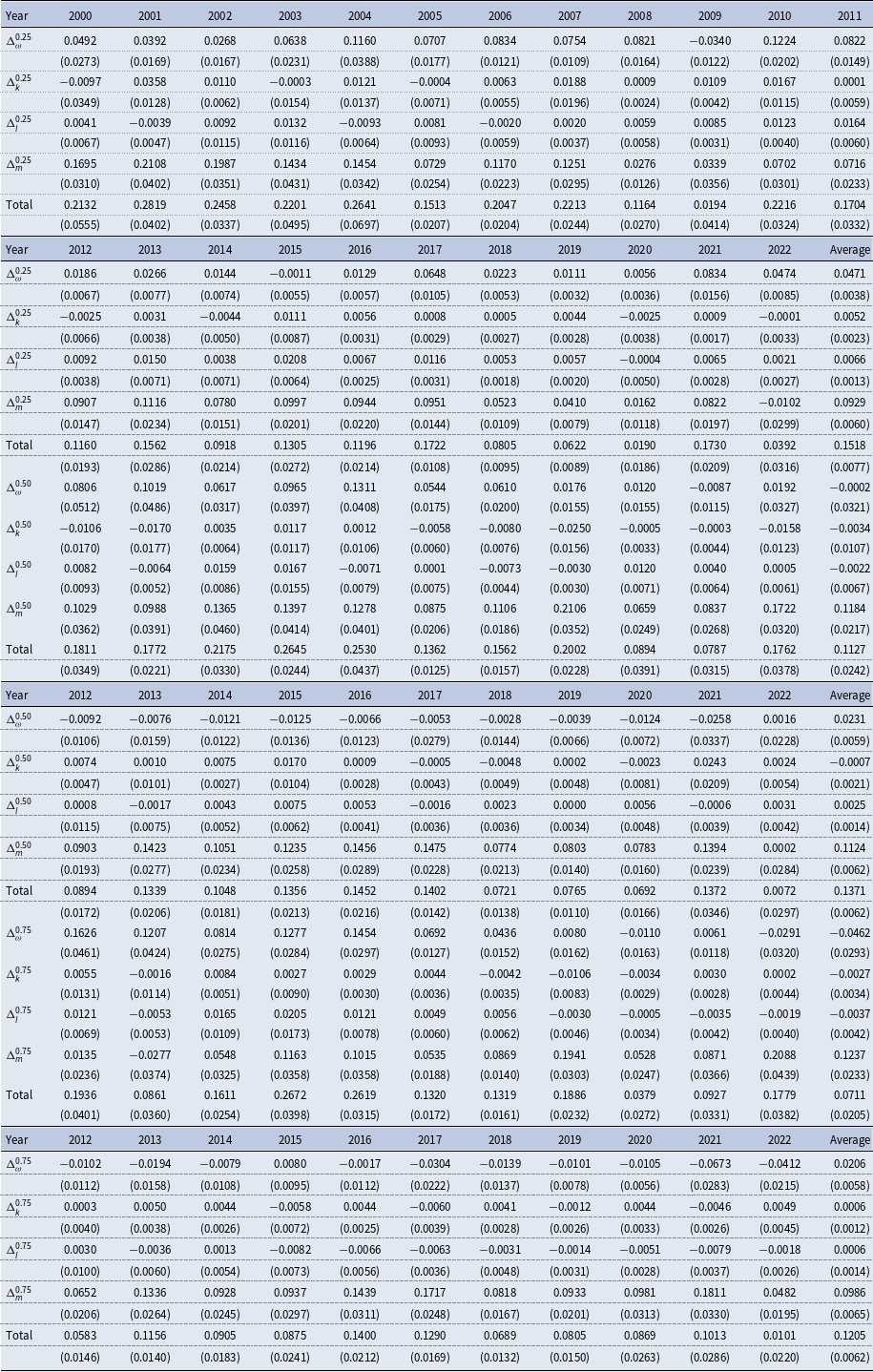
Specifically, our quantile decomposition of output growth among listed Chinese manufacturing firms focuses on the first, second (median), and third quartiles of the output distribution. They are chosen to represent the small-, median-, and large-sized firms, respectively. The corresponding results are summarized in Table 4 and visualized in Figure 3.
Output quartile decomposition

Notes: We report results from quantile decomposition at the 1st, median, and 3rd quartiles of the output distribution. Column “Total” refers to the average annual output growth rate of listed manufacturing firms in the corresponding period at each quartile (
 $\tau$
), and it equals the sum of the contributions from productivity progress (
 $\Delta _\omega ^\tau$
), capital (
 $\Delta _k^\tau$
), labor (
 $\Delta _l^\tau$
), and materials (
 $\Delta _m^\tau$
) deepening. Row “Average” shows the averages of the entire sample period from 2000 to 2022. Standard errors of cross-industry mean estimates are reported in parentheses.
Similar to the analysis of the mean decomposition, we divide the entire sample period into four sub-periods and report the average annual quartile decomposition for each sub-period in Table 4. Additionally, for detailed insights, we provide the decomposition results for each year in Tables A1 and A2 of the appendix.
There are a few noteworthy findings from our analysis. First, in each period, we observe a decrease in output growth rate as firm size increases, progressing from the first quartile to the median, and finally to the third quartile of the output distribution. The gap of output growth between large and small firms gets narrower over time. Second, within each quartile, we find that production growth rate peaks during the period 2000-2007, followed by 2013–2017, 2008–2012, and 2018–2022, respectively. Third, our analysis, illustrated in Figure 3, highlights significant contributions of productivity progress to output growth before the 2008 financial crisis, which are evident across firms of all sizes. Notably, larger firms exhibit higher productivity growth, which contributes more to their output growth, during the period 2000–2007. However, this trend undergoes a dramatic shift in subsequent periods. Specifically, we observe that only small firms in the first quartile continue to display significant productivity growth in certain years post-2009. For median-sized firms, the contribution of productivity progress to output growth approaches zero after 2009, while for large firms in the third quartile, this contribution even becomes negative.
Overall, our findings indicate a notable shift in output growth dynamics for median and large manufacturing firms over time. Specifically, we observe that their growth is primarily fueled by increases in materials usage rather than advancements in firm productivity in recent years. This shift underscores the need for policies focusing on fostering innovation and creativity, particularly among larger firms, to sustain long-term industrial growth. This dynamic evolution of productivity and input contributions to output growth and the heterogeneity among firms of different sizes constitute a novel contribution to the literature. Previous studies, such as Huang et al. (Reference Huang, Zhao and Kumbhakar2022), which rely on Chinese industrial survey data, have primarily focused on the period before the 2008 financial crisis. Our empirical results demonstrate distinct growth patterns among Chinese manufacturing firms before and after the crisis.
Output quartile decomposition. Notes:
 $\omega$
,
 $k$
,
 $l$
, and
 $m$
refer to the contributions from productivity, capital, labor, and materials to output growth, respectively.

5.2 Productivity growth decomposition
5.2.1. O-P decomposition
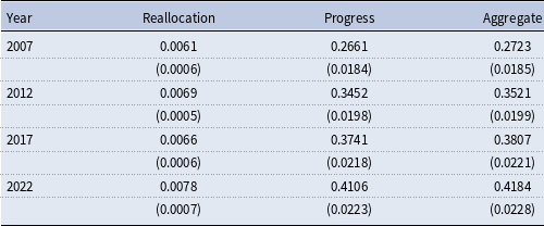
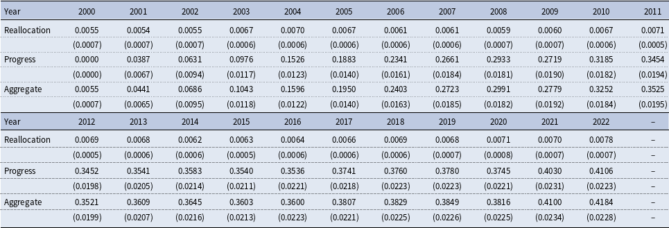
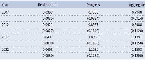
In this section, we present productivity decomposition for listed manufacturing firms in China over our sample period. We begin our analysis with a simple static (O-P, Olley and Pakes, Reference Olley and Pakes1996) decomposition following Equation (3.7), with summarized results presented in Table 5. For easier interpretation, we normalize the estimated
 $\{\omega _{it}\}$
series by subtracting an industry-specific constant, ensuring its average in the first year of our sample period (2000) is zero. After this normalization, the values reported in columns “Progress” and “Aggregate” of the table can be interpreted as cumulative productivity growth since 2000. Additionally, in Table 5, we report the last-year value for each of the four sub-periods discussed earlier. For the detailed year-by-year decomposition results, please refer to Table A3 in the appendix.
Industry productivity decomposition

Notes: Industry aggregate productivity decomposition follows Equation (3.7). Column “Reallocation” refers to the covariance between firms’ output share and productivity, column “Progress” refers to the unweighted mean of firm productivity, and column “Aggregate” refers to the industry aggregate productivity, which is the sum of the previous two columns. Standard errors of cross-industry mean estimates are reported in parentheses.
We have the following two key findings from Table 5. First, similar to the pattern of output growth, Chinese listed firms exhibit their fastest productivity growth during the period 2000-2007, with cumulative industry aggregate productivity growth reaching 27.23% over 8 years, translating to an average annual growth rate of 3.40%. In the subsequent 5-year period (2008–2012), encompassing the financial crisis, productivity growth slows considerably, yielding a cumulative industry aggregate productivity growth of 7.98% (35.21–27.23%), with an annual growth rate of 1.60%. Following this, we observe a further deceleration in productivity growth in later years: cumulative industry aggregate productivity growth stands at 2.86% (38.07–35.21%) during 2013–2017 and 3.77% (41.84–38.07%) during 2018–2022, corresponding to annual growth rates of 0.572% and 0.754%, respectively. These results align with the output decomposition results in Tables 3 and 4, which shows a diminishing contribution of productivity progress to overall output growth over time. However, also note that Chinese listed firms exhibit significant variation in productivity growth across individual years, even within each sub-period. We can see the unsmooth pattern from the detailed year-by-year decomposition results in Table A3 of the appendix.
Second, our analysis reveals that across all sub-periods, industry aggregate productivity growth is predominantly driven by the productivity progress term, while the contribution from output reallocation efficiency remains limited. Remember that the productivity progress is defined as the unweighted average of firm productivity, and the reallocation efficiency measures the covariance between firms’ output share and productivity. This result suggests that, despite a notable overall increase in productivity by 41.84% over the past 23 years, the market shares of the most productive firms have not shown significant improvement. This phenomenon can be attributed to two main factors. On the one hand, the continuous influx of new firms into the markets each year intensifies competition and may dilute the market shares of all existing firms. On the other hand, although the entire Chinese manufacturing sector has experienced rapid expansion, the variation in output growth among firms of different productivity levels may not be substantial. Consequently, the overall improvement in reallocation efficiency, as measured by changes in market share, remains limited.
5.2.2. Ownership decomposition
The Olley and Pakes (Reference Olley and Pakes1996) decomposition presented above focuses on the cumulative productivity growth of listed Chinese manufacturing firms over our sample period. However, it offers only indirect evidence of annual productivity growth and does not illustrate the effects of firms’ ownership on productivity. Among state-invested, foreign-invested, and domestic firms, which one has the largest contribution to China’s productivity advancement? Do foreign firms, believed to bring advanced production technologies and better management skills to China, grow faster than domestic firms in alien lands? Do state firms, conventionally regarded as less efficient, slow down China’s growth? To answer these and related questions, we next delve into a more detailed examination of industry aggregate productivity growth decomposition by ownership, following Equation (3.8).
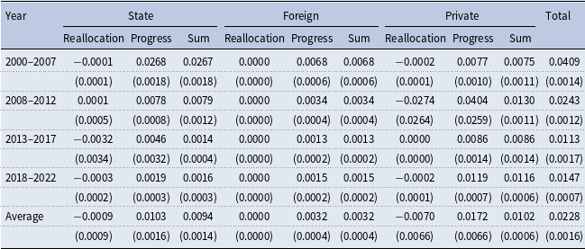
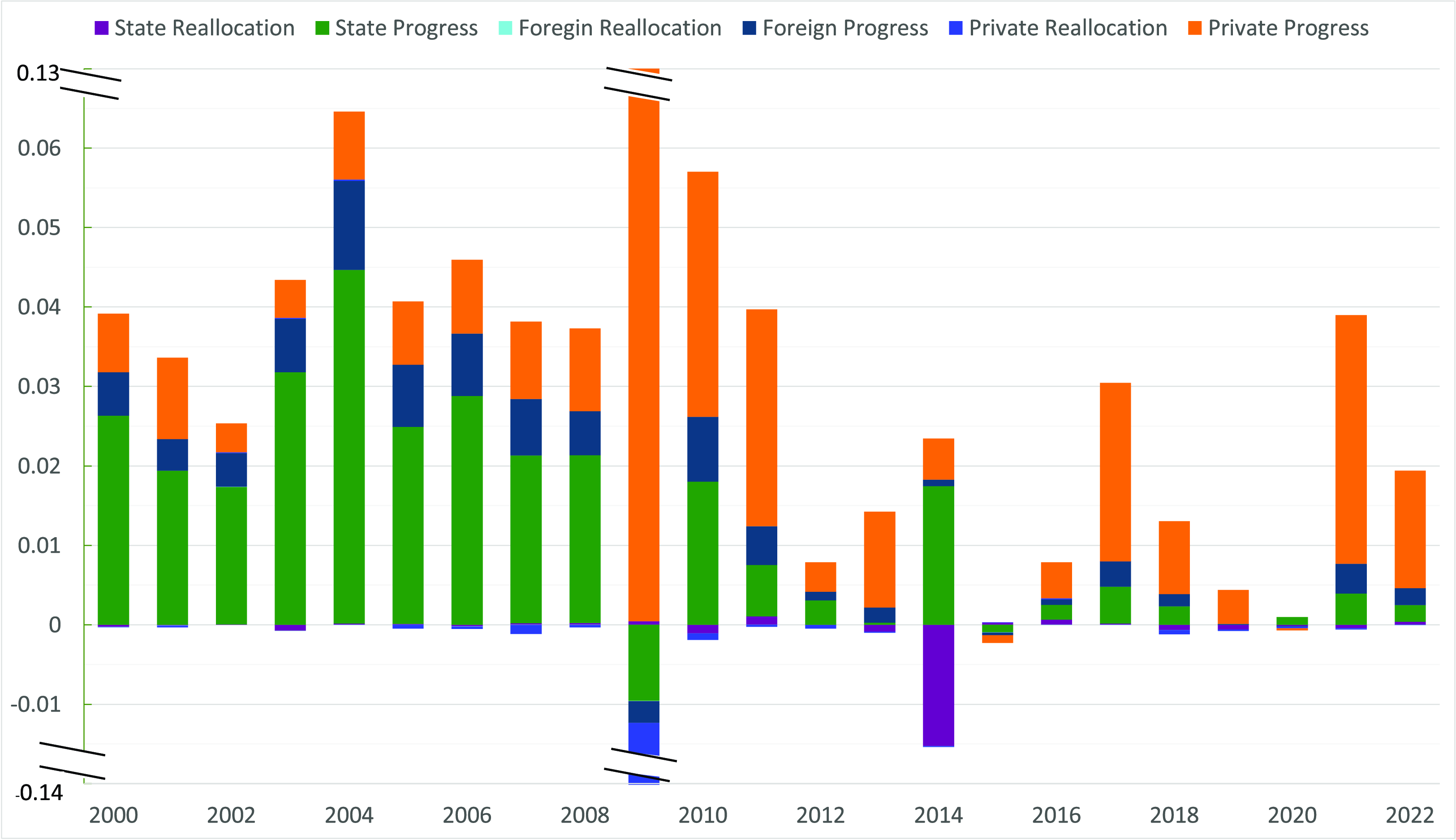
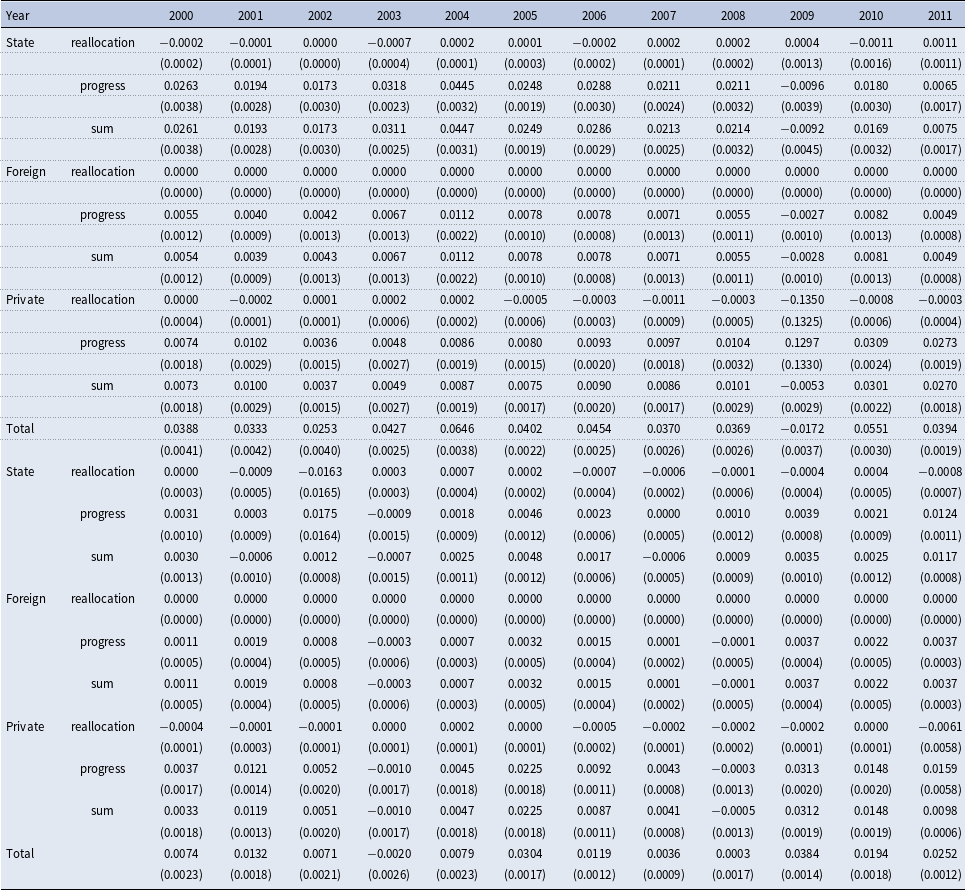
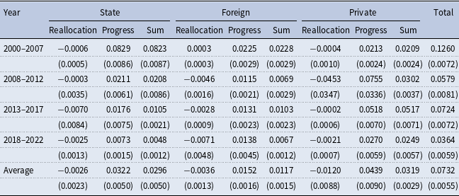
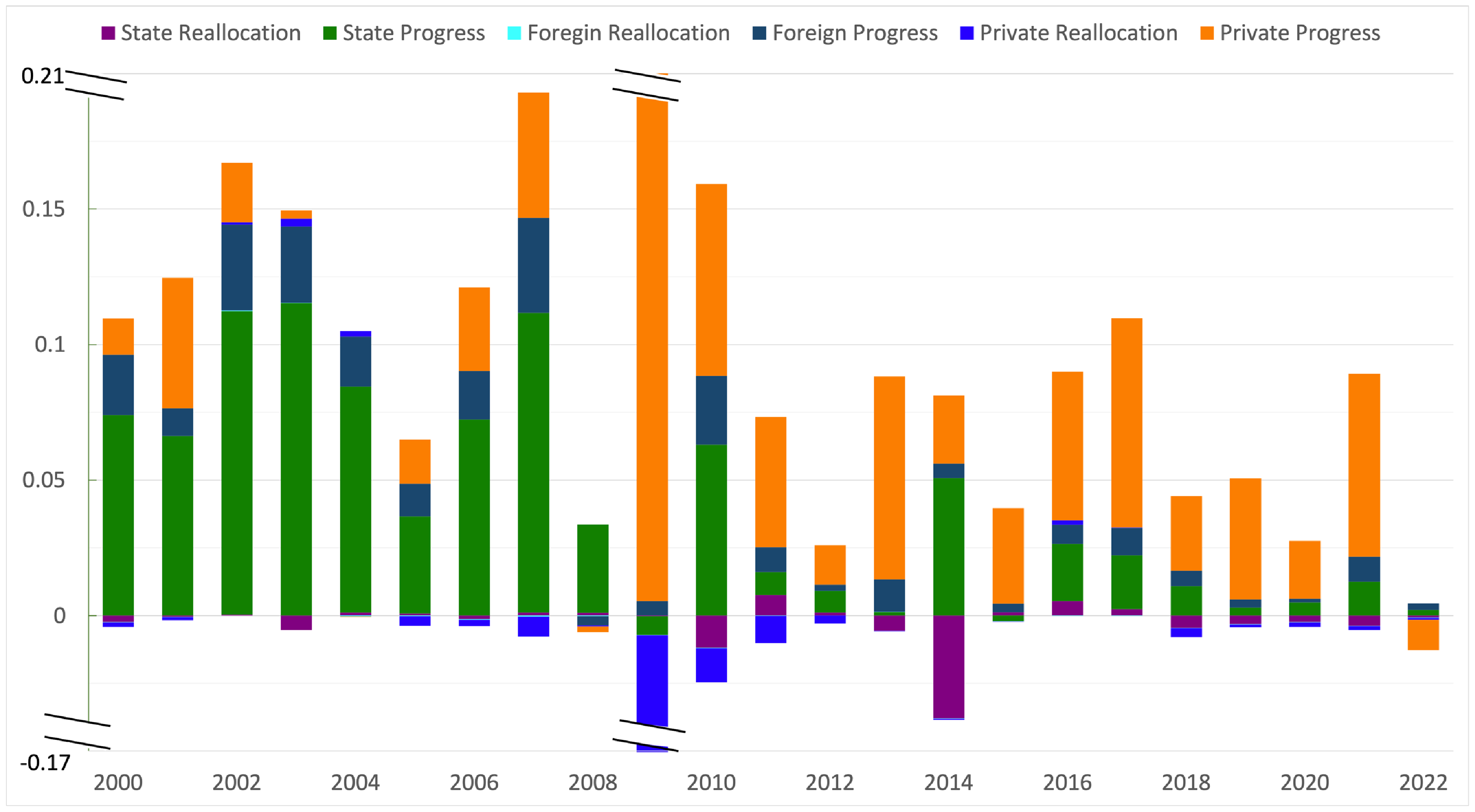
The results are summarized in Table 6 and visualized in Figure 4. In Table 6, we report the average contribution of output reallocation efficiency improvement and productivity progress to the annual industry productivity growth for each type of firms and in each of the four sub-periods. Further sights into the year-by-year decomposition can be found in Table A4 of the appendix. Additionally, Figure 4 provides the year-by-year evidence using bar plots.
Productivity decomposition by ownership

Notes: Industry aggregate productivity decomposition follows Equation (3.8). Column “Reallocation” refers to output reallocation efficiency improvement, column “Progress” refers to unweighted average productivity changes, and column “Sum” refers to the sum of the previous two. Standard errors of cross-industry mean estimates are reported in parentheses.
Productivity decomposition - state, foreign, private. Notes: State/Foreign/Private Reallocation and State/Foreign/Private Progress refer to the ownership-specific output reallocation efficiency improvement and unweighted average productivity changes, respectively.

The productivity dynamics within China’s manufacturing sector, as highlighted by our analysis, underscore some key trends in the relative contributions of various firm types (state-invested, foreign-invested, and domestic private firms) across distinct phases of economic development. First, consistent with the findings of the above O-P decomposition, the contribution of output reallocation to industry productivity growth is close to zero for all three types of firms and in all periods. This suggests that, compared with their less productive counterparts, the more productive state-invested, foreign-invested, and domestic private firms did not necessarily increase their market shares in China during our sample period.
Second, we observe that in the first period from 2000 to 2007, the average annual productivity growth is 4.09%, and the largest contribution comes from the productivity progress of state-invested firms. This may reflect the effects of the continuation of economic reforms among state firms in China at the beginning of the twenty-first century. During this period, smaller and less productive state firms were privatized, merged, or replaced by more productive private firms. The remaining state firms were larger, crucial for China’s economy, and more productive in general. The faster growth rate of state firms compared with other types of firms in this period has also been documented by previous studies, such as Hsieh and Song (Reference Hsieh and Song2015) and Zhao et al. (Reference Zhao, Qian and Kumbhakar2020). For foreign-invested and domestic private firms, they have similar contributions to industry productivity growth in this period.
Third, in the second period from 2008 to 2012, the importance of state-invested firms to industry productivity growth gradually declines, while the productivity progress of domestic private firms becomes the main contributor. In this period, the average annual industry productivity growth rate remains relatively high at 2.43%. However, there is a significant efficiency loss immediately following the 2008 financial crisis, attributed to a productivity decrease among state-invested firms and a deterioration in reallocation efficiency among private firms. This likely reflects market adjustments toward a new equilibrium after the financial crisis.
Fourth, in the third period spanning 2013–2017, Figure 4 shows two noticeable spikes in industry aggregate productivity growth in 2014 and 2017, which are attributed respectively to the productivity progress of the state-invested and domestic private firms. In other years of this period, industry aggregate productivity growth is low. In the final period from 2018–2022, the productivity progress of domestic private firms continues to be the only significant driver of industry productivity growth. During the 2019–2020 pandemic years, with stringent controls, the industry productivity growth is close to zero.
Overall, these findings highlight the evolution of productivity growth within China’s manufacturing sector, with different firm types taking on varying roles across different economic phases. The limited role of reallocation efficiency, coupled with the declining productivity contributions from state-invested firms and the increasing importance of domestic private firms, reflects broader structural changes in the Chinese economy over the past two decades. These dynamics suggest a need for policy measures that enhance market mechanisms, ensuring that more productive firms can expand and drive industry-wide productivity improvements.
6. Conclusion
In this paper, we investigate the sources of output and productivity growth among China’s listed manufacturing companies from 2000–2022. Based on the different economic conditions and varying growth rates, we divide the entire sample period into four sub-periods. Within each sub-period, we decompose output growth into contributions from input deepening and productivity progress at both the mean and various quantiles of the output distribution. Our findings reveal that output growth gradually slows down post the 2008 financial crisis, and the increase in materials usage and productivity growth are the primary growth drivers. However, the contribution of productivity growth exhibits a notable decline in recent years, particularly between 2013 and 2017 and for median-sized and large firms. We observe significant heterogeneity among firms of different sizes, as measured by output. Smaller firms demonstrate swifter output growth compared to larger ones, and they tend to have more persistent productivity growth. Regarding aggregate industry productivity, our findings underscore the significant role of economic forms among state firms in driving growth pre-2008 financial crisis. While China’s growth has slowed down in recent years, domestic private firms continue to make large contributions to industry productivity advancement relative to state- and foreign-invested firms. Nonetheless, our analysis reveals no substantial evidence of output reallocation efficiency improvement in China throughout our sample period.
Our findings on China’s post-2008 slowdown in output and productivity growth, particularly among larger and state-invested firms, suggest a need to reevaluate current economic policies. Targeted support for smaller, domestic private firms that have shown sustained productivity growth should be considered. Policymakers should focus on creating a competitive environment and fostering innovation within these firms to help mitigate the overall productivity decline. Additionally, given the potential inefficiency in resource distribution across firms, policies aimed at enhancing market-driven reallocation processes and promoting fair competition could be instrumental in revitalizing China’s productivity growth. These measures may support long-term economic development by ensuring that more productive firms, regardless of size and ownership structure, can expand and thrive in a competitive market.
Acknowledgment
Xie: This paper is partially supported by China National Social Science Fund: The Economic Value and Empirical Research of Chinese Digitization Popularization and Application from the Perspective of Linguistic Economics (project number: 23FJLB024).
Competing interests
The author(s) declare none.
Appendix A. Additional data description
The data for this study are primarily sourced from the China Stock Market Accounting Research (CSMAR). The Chinese stock market comprises three types of stocks: A, B, and H shares. A and B shares are transacted in mainland China. A shares, denominated in RMB, are exclusively traded by Chinese citizens. B shares, denominated in US dollars on the Shanghai Stock Exchange (SHSE) and in HK dollars on the Shenzhen Stock Exchange (SZSE), were initially limited to foreign investors until February 2001. Since then, Chinese citizens with deposit accounts in foreign currencies have been allowed to trade B shares. H shares are traded on the Stock Exchange of Hong Kong and denominated in HK dollars. For the purposes of this study, we focus on A market manufacturing firms.
We compile information from two databases provided by the China Listed Firms research in CSMAR, following the methodologies of Wang (Reference Wang2010), Li et al. (Reference Li, Lu, Mittoo and Zhang2015), Du et al. (Reference Du, Boateng and Newton2016), Ma et al. (Reference Ma, Sun, Waisman and Zhu2016), He and Kyaw (Reference He and Kyaw2018), Rathnayake et al. (Reference Rathnayake, Kassi, Louembe, Sun and Ding2019), and others. Our data collection encompasses firm operating and performance details from two main sources: (1) the Financial Statement databaseFootnote 8 (which includes tables of balance sheet, income statement, and an indirect method statement of cash flow), and (2) the Corporate Governance database (which includes tables of general information on corporate governance, capital structure, and basic information on the company profile).
Below, we list the raw variables along with the tables available in the databases:
-
• Financial Statement Database (FS): The FS database compiles all financial data, including annual, interim, and quarterly reports, of A-share and B-share companies across various industries listed on the Shanghai Stock Exchange, the Shenzhen Stock Exchange, and the Beijing Stock Exchange since 1990. This study specifically concentrates on the A-share market. In the balance sheet table, we collect two variables along with the company’s stock code, stock type, and year information: Net Fixed Asset, denoted as the net amount of fixed assets after deducting accumulated depreciation and impairment provision, and Employee Compensation Payable, representing all forms of compensation provided by an enterprise to employees as stipulated. This can be calculated based on wages and salaries, staff welfare, social insurance contributions, housing funds, union running costs, employee education costs, non-monetary benefits, termination benefits, share-based payment, etc. In the income statement table, we collect the following variables along with firm identification information: Operating Revenue (refers to the operating revenue confirmed by the company during its operation), Operating Costs (denoted as the operating costs confirmed by the enterprise), Selling Expenses (expenses incurred by an enterprise in the sales of products, including expenses involved in transportation, loading and unloading, packaging, insurance, exhibition, advertising, etc.), and Administrative Expense (expenses incurred by an enterprise in organizing and managing its production and operation). The variables are denoted in current year RMB prices. In the table of statement of cash flow (indirect method), we collect depreciation of fixed assets, oil and gas assets, and bearer biological assets.
-
• The Corporate Governance (CG) database contains information on the top 10 shareholders, shareholders’ meetings, executive profiles, changes in the chairman of the board and general managers, and changes in equity disclosed by companies listed on the Shanghai and Shenzhen stock exchanges since 1999. In the table of general information on corporate governance, we collect the number of employees, which is the total number of employees of the listed company, and the number of registered employees, referring to the number of in-service employees of the listed company disclosed in the annual report. In the table of capital structure, we collect the total number of shares, the total number of non-negotiable shares (including state-owned shares and foreign promoters’ shares), and the total number of negotiable shares (including negotiable A shares, B shares, H shares, and the number of other overseas negotiable shares). In the table of basic information of the company profile, we collect the industry classification code.
-
• Additionally, we deflate all monetary values using price indices from the China Economic Research Series database. Specifically, we use the Macroeconomic database-Price indices-General price indices (1990 = 100) table, collecting the ex-factory price index of industrial products (1990 = 100), purchasing price index of raw material, fuel and power (1990 = 100), and the price index of investment in fixed assets (1990 = 100). We also utilize the GDP deflator from the Series of Gross Domestic Product Indices (1990 = 100) table. After deflation, monetary values, such as
 $Y, K, M$
, are expressed in hundreds of RMB at 1990 prices.

Appendix B. Identification and estimation of production function
In this section, we briefly explain the identification and estimation of the firm’s production function and productivity for the purpose of conducting the decomposition in the main text. The identification part mainly follows Gandhi et al. (Reference Gandhi, Navarro and Rivers2020). We propose a nonparametric production function that accounts for the substantial heterogeneity of firm’s production technology and a fast turnover rate.
B.1. Identification
Following Olley and Pakes (Reference Olley and Pakes1996), we assume that firms have both long-run dynamic optimization and short-run static problems. In the former case, we assume that
 $K_{it}$
and
 $L_{it}$
are determined at time
 $t-1$
. In the latter case, a firm maximizes its current period profit by choosing the optimal level of the materials input conditional on predetermined
 $K_{it}$
and
 $L_{it}$
. A similar assumption is also made by Gandhi et al. (Reference Gandhi, Navarro and Rivers2020), Malikov et al. (Reference Malikov, Zhao and Kumbhakar2020), and Huang et al. (Reference Huang, Zhao and Kumbhakar2022).
Annual output quartile decomposition

Notes: We report quartile decomposition at the 1st, median, and 3rd quartiles of the output distribution. Row “Total” refers to the output growth rate of listed manufacturing firms in the corresponding year at each quartile (
 $\tau$
), and it equals the sum of the contributions from productivity (
 $\Delta _\omega ^\tau$
), capital (
 $\Delta _k^\tau$
), labor (
 $\Delta _l^\tau$
), and materials (
 $\Delta _m^\tau$
). Column “Average” shows the averages between 2000 and 2023. Standard errors of cross-industry mean estimates are reported in parentheses.
Industry productivity decomposition

Notes: Industry aggregate productivity decomposition follows Equation (3.7). Row “Reallocation” refers to the covariance between firms’ output share and productivity, row “Progress” refers to the unweighted mean of firm productivity, and row “Aggregate” refers to the industry aggregate productivity, which is the sum of the previous two rows. Standard errors of cross-industry mean estimates are reported in parentheses.
Annual industry productivity decomposition by ownership

Notes: Industry aggregate productivity decomposition follows Equation (3.8). Row “Reallocation” refers to the covariance between firms’ output share and productivity, row “Progress” refers to the unweighted mean of firm productivity, row “Sum” refers to the sum of the previous two rows, and row “Total” refers to industry aggregate productivity growth. Standard errors of cross-industry mean estimates are reported in parentheses.
Let
 $\Omega _{it}$
be the information set for firm
 $i$
at time
 $t$
. In Equation (3.1),
 $\omega _{it} \in \Omega _{it}$
is known to the firm at time
 $t$
but unobservable to econometricians. Therefore,
 $\omega _{it}$
is correlated with materials input usage. We assume
 $\omega _{it}$
follows a controlled first-order Markov process with a distribution of
 $P_{\omega }(\omega _{it}|\Omega _{it-1})=P_{\omega }(\omega _{it}|\omega _{t-1}, z_{it-1})$
. For our application,
 $z_{it-1}$
includes two ownership variables: the share of foreign equity (
 $sF$
) and the share of state equity (
 $sS$
). The choice of
 $z_{it-1}$
, following Huang et al. (Reference Huang, Zhao and Kumbhakar2022), reflects our belief that foreign, state, and private firms have different incentives to improve their productivity. In contrast to
 $\omega _{it}$
,
 $\eta _{it}$
is an i.i.d.,
 $P_{\eta }(\eta _{it}|\Omega _{it})=P_{\eta }(\eta _{it})$
, random productivity shock that is out of the firm’s control.
Building on Gandhi et al. (Reference Gandhi, Navarro and Rivers2020) and Olley and Pakes (Reference Olley and Pakes1996), we propose a two-step process to estimate the nonparametric production function and persistent productivity.
Step 1: Consider the following static profit maximization problem of firm
 $i$
:
 \begin{align*} \pi _{it}(K_{it}, L_{it}, \omega _{it})=\max _{M_{it}} \ P_{it} \ G(K_{it}, L_{it}, M_{it})e^{\omega _{it}} \Lambda - P_{M,it} M_{it}, \end{align*}
where
 $P_{it}$
is the price of output,
 $P_{M,it}$
is the price of the intermediate input (materials), and
 $\Lambda =E\left (e^{\eta _{it}} \right )$
. The first-order condition of the optimization problem is:
 \begin{equation} \ln{s_{M,it}} =\ln \left ( \beta _{M}(K_{it}, L_{it}, M_{it})\Lambda \right ) -\eta _{it}, \end{equation}
where we denote the share of materials by
 $s_{M,it}$
and the output elasticity of materials by
 $\beta _{M}(K_{it}, L_{it},$
 $M_{it})$
. In Equation (B.1), the left-hand side can be calculated directly from the data, and this equation is simply a standard nonparametric regression with the arguments
 $K_{it}$
,
 $L_{it}$
, and
 $M_{it}$
plus an error term
 $(-\eta _{it})$
. Since
 $\eta _{it}$
is uncorrelated with variables determined in period
 $t$
, we can estimate
 $\ln (\beta _{Mt}(K_{it}, L_{it}, M_{it})\Lambda )$
and
 $\eta _{it}$
using the moment conditions,
 \begin{equation} E(\eta _{it}|K_{it}, L_{it}, M_{it})=0. \end{equation}
Therefore, we can recover
 $\Lambda =E\left (e^{\eta _{it}} \right )$
and the elasticity
 $\beta _{M}(K_{it}, L_{it}, M_{it})$
.
Note that under the assumption of perfectly competitive markets, where
 $P_{M,it}$
and
 $P_{it}$
are constant across firms, the above profit maximization problem implies that the materials input demand
 $M_{it}$
can be written as a function of
 $K_{it}$
,
 $L_{it}$
,
 $\omega _{it}$
. Petrin and Levinsohn (Reference Petrin and Levinsohn2012) further show that under some regularity assumptions of the production function,
 $M_{it}$
is monotonically increasing in
 $\omega _{it}$
. By inverting the materials demand function, we can express the persistent productivity in terms of the inputs, that is,
 \begin{equation} \omega _{it} = M_t^{-1}(K_{it}, L_{it}, M_{it}). \end{equation}
This equation carries the key idea in the literature on estimation of production functions using the proxy variable method.
Step 2: Since
 $\frac{\beta _{M}(K_{it}, L_{it}, M_{it})}{M_{it}}=\frac{\partial }{\partial M_{it}} \ln G(K_{it}, L_{it}, M_{it})$
, by the fundamental theorem of calculus, we have
 \begin{equation} \int \frac{\beta _{M}(K_{it}, L_{it}, M_{it})}{M_{it}} dM_{it}=\ln G(K_{it}, L_{it}, M_{it}) + \phi (K_{it}, L_{it}). \end{equation}
The left-hand-side of Equation (B.4) can be calculated based on the estimated
 $\beta _{M}$
which is obtained from the first step. Therefore, the production function
 $G(K_{it}, L_{it}, M_{it})$
is identified if
 $\phi (K_{it}, L_{it})$
is identifiable. By taking the difference between the log production function (3.2) and Equation (B.4), we have
 \begin{equation} \mathcal{Y}_{it} \equiv \ln Y_{it}-\int \frac{\beta _M(K_{it}, L_{it}, M_{it})}{M_{it}} dM_{it}-\eta _{it}=-\phi (K_{it}, L_{it})+\omega _{it}. \end{equation}
The left-hand side, denoted by
 $\mathcal{Y}_{it}$
, is either observed or estimated in the first step. Thus,
 $\phi (K_{it}, L_{it})$
can be obtained from the estimation of the above equation. Taking the conditional expectation of both sides of Equation (B.5) for the observed firms, we have
 \begin{align} E(\mathcal{Y}_{it}|\Omega _{it-1}) =& -\phi (K_{it}, L_{it}) + E(\omega _{it}| \omega _{it-1}, z_{it-1}) \nonumber \\ =& -\phi (K_{it}, L_{it})+\varphi _t(K_{it-1}, L_{it-1}, M_{it-1}, z_{it-1}), \end{align}
where
 $\varphi _t(K_{it-1}, L_{it-1}, M_{it-1}, z_{it-1}) = \psi (Q_t^{-1}(K_{it-1},L_{it-1},M_{it-1},z_{it-1}), M_t^{-1}(K_{it-1},L_{it-1}, M_{it-1}),{} z_{it-1})$
, and the inverse materials demand function (B.3) is used. Letting
 $\xi _{it}$
be the innovation in
 $\omega _{it}$
at period
 $t$
, the above equation suggests
 \begin{equation} \mathcal{Y}_{it}=-\phi (K_{it}, L_{it})+\varphi _t(K_{it-1}, L_{it-1}, M_{it-1}, z_{it-1}) +\xi _{it}. \end{equation}
By definition, we have
 $E(\xi _{it}|\Omega _{it-1})=0$
, that is,
 $\xi _{it}$
is uncorrelated with all right-hand-side variables in Equation (B.7). The unknown function
 $\phi ({\cdot})$
, as well as
 $\varphi _t({\cdot})$
, can be estimated from the following conditional moment conditions:
 \begin{equation} E(\xi _{it}|\Omega _{it-1})=E(\xi _{it} | K_{it},L_{it}, K_{it-1}, L_{it-1}, M_{it-1}, z_{it-1})=0. \end{equation}
Thus, we can recover the production function from Equation (B.4). Also, given the estimated
 $\eta _{it}$
and
 $G({\cdot})$
, we can calculate
 $\omega _{it}$
from
 \begin{equation} \omega _{it} = \ln{Y_{it}} - \ln G(K_{it}, L_{it}, M_{it}) - \eta . \end{equation}
B.2. Estimation
To obtain firm productivity and perform our proposed decomposition, we need to estimate a few production-function-related nonparametric regressions, that is, Equations (B.1), (B.7). In this section, we provide detailed steps for their estimation.
B.2.1. Production function estimation
To obtain estimates of the production function and productivity, we need to estimate Equations (B.1) and (B.7). Following Gandhi et al. (Reference Gandhi, Navarro and Rivers2020), we use the method of sieves and approximate all unknown functions with polynomial bases.
Specifically, to estimate Equation (B.1), we approximate the materials elasticity in the following way:
 \begin{equation} \beta _{M}(K_{it}, L_{it}, M_{it})\Lambda \approx \sum _{j_k+j_l+j_m \leq 2} \theta _{\beta _{M},j_k,j_l,j_m} k_{it}^{j_k}l_{it}^{j_l}m_{it}^{j_m}. \end{equation}
According to the moment condition
 $E(\eta _{it}|K_{it}, L_{it}, M_{it})=0$
, the coefficients
 $\theta$
, as well as
 $\eta _{it}$
, are estimated from the following ordinary least squares problem:
 \begin{equation} \widehat{\theta }_{\beta _{M}} =\arg \min _{\theta _{\beta _{M}}} \frac{1}{NT}\sum _{i=1}^{N}\sum _{t=1}^{T}\left ( \ln s_{M,it} - \ln \left ( \sum _{j_k+j_l+j_m \leq 2} \theta _{\beta _{M},j_k,j_l,j_m} k_{it}^{j_k}l_{it}^{j_l}m_{it}^{j_m} \right ) \right )^2, \end{equation}
where
 $\theta _{\beta _{M}} = \{\theta _{\beta _{M},j_k,j_l,j_m}: j_k+j_l+j_m \leq 2\}$
. We can recover
 $\widehat{\beta }_{M}(K_{it}, L_{it}, M_{it})$
by dividing both sides of Equation (B.10) by
 $\widehat{\Lambda }$
, where
 $\widehat{\Lambda }=\frac{1}{NT}\sum _{i=1}^{N}\sum _{t=1}^{T}e^{\widehat{\eta }_{it}}$
. Then, its integral has a closed-form solution, which is
 \begin{equation} \int \frac{\widehat{\beta }_{M}(K_{it}, L_{it}, M_{it})}{M_{it}} dM_{it} = \sum _{j_k+j_l+j_m \leq 2} \frac{\widehat{\theta }_{\beta _{M},j_k,j_l,j_m}}{(j_m + 1) \widehat{\Lambda }} k_{it}^{j_k}l_{it}^{j_l}m_{it}^{j_m+1}. \end{equation}
The value obtained from the above equation is further used to calculate
 $\mathcal{Y}_{it}$
.
Equation (B.7) is a standard nonparametric additive regression model. We approximate
 $\phi ({\cdot})$
and
 $\varphi _t({\cdot})$
using second-order polynomials of their respective arguments. Define
 $v_{it}^{\phi } = (k_{it}, l_{it})'$
and
 $v_{it-1}^{\varphi } = (k_{it-1}, l_{it-1}, m_{it-1}, z_{it-1})'$
. Then,
 \begin{align*} &\phi (K_{it}, L_{it}) \approx \mathcal{P}_2(v_{it}^{\phi }) \ \theta _{\phi }, \\ &\varphi _t(K_{it-1}, L_{it-1}, M_{it-1}, z_{it-1}) \approx \mathcal{P}_2(v_{it-1}^{\varphi }) \ \theta _{\varphi }, \end{align*}
where
 $\theta _{\phi }$
and
 $\theta _{\varphi }$
are vectors of coefficients with compatible dimensions.Footnote
9
These coefficients are estimated from minimizing the sum of squared residuals:
 \begin{equation} (\widehat{\theta }_{\phi }, \widehat{\theta }_{\varphi }) = \arg \min _{\theta _{\phi }, \theta _{\varphi }} \frac{1}{NT}\sum _{i=1}^{N}\sum _{t=1}^{T}\Big (\mathcal{Y}_{it}+\mathcal{P}_2(v_{it}^{\phi }) \ \theta _{\phi }-\mathcal{P}_2(v_{it-1}^{\varphi }) \ \theta _{\varphi }\Big ). \end{equation}
Appendix C. Additional empirical results
In this appendix, we report additional empirical results mentioned in the main text. They are detailed, year-by-year output growth quantile decomposition, simple O-P industry aggregate productivity decomposition, and industry aggregate productivity decomposition by ownership.
Industry productivity decomposition with value-added method

Notes: Industry aggregate productivity decomposition follows Equation (3.7) based on the productivity calculation from Ackerberg et al. (Reference Ackerberg, Caves and Frazer2015). Column “Reallocation” refers to the covariance between firms’ output share and productivity, column “Progress” refers to the unweighted mean of firm productivity, and column “Aggregate” refers to the industry aggregate productivity, which is the sum of the previous two columns. Standard errors of cross-industry mean estimates are reported in parentheses.
Appendix D. Robustness check
In the main text, we estimate firm productivity from a gross production function following Gandhi et al. (Reference Gandhi, Navarro and Rivers2020). As a popular alternative, one can estimate productivity from a value-added production function following Ackerberg et al. (Reference Ackerberg, Caves and Frazer2015). In this appendix, we compare the aggregate productivity decomposition results generated from a value-added production function with those from the benchmark model in Section 5.2 as a robustness check.
For the OP decomposition outlined in Equation (3.7), Table A5 reports the last-year value for each of the four sub-periods discussed earlier, echoing Table 5 in the main text. Since we normalize the estimated
 $\omega$
to ensure that its mean in year 2000 is zero, the values reported in columns “Progress” and “Aggregate” are the cumulative productivity growth since 2000. Similar to the patterns in Table 5, we have the following two key findings.
First, Chinese listed firms exhibit their fastest productivity growth during the period 2000–2007. The value-added method generates larger values than those in the benchmark model, with cumulative industry aggregate productivity growth reaching 79.48% over 8 years (compared to 27.23% reported in the main text) and an annual average of 9.94% (compared to 3.40% reported in the main). In the subsequent 5-year period (2008–2012), due to the financial crisis, productivity growth slows, with aggregate productivity growth decreasing to 10.4% (7.98% in the main text) and an annual average of 2.08% (2.86% in the main text). Unlike in the main text, we do not observe a persistent deceleration in the third sub-period. Instead, we first observe an acceleration in productivity growth—cumulative industry aggregate productivity growth reaches 24.03% (113.91–89.88%) during 2013–2017, with a 4.81% annual growth rate (0.572% in the main text). This is followed by a deceleration to 1.12% (115.03–113.91%) during 2018–2022, with an annual growth rate of 0.22% (0.754% in the main text). These results largely echo those in Table 5, suggesting a diminishing contribution of productivity progress to overall output growth over time.
Productivity decomposition by ownership with value-added method

Notes: Industry aggregate productivity decomposition follows Equation (3.8), based on the productivity calculation from Ackerberg et al. (Reference Ackerberg, Caves and Frazer2015). Column “Reallocation” refers to output reallocation efficiency improvement, column “Progress” refers to unweighted average productivity changes, and column “Sum” refers to the sum of the previous two. Standard errors of cross-industry mean estimates are reported in parentheses.
Value-added productivity decomposition - state, foreign, private. Notes: State/Foreign/Private Reallocation and State/Foreign/Private Progress refer to the ownership-specific output reallocation efficiency improvement and unweighted average productivity changes, respectively. The productivity calculation is based on Ackerberg et al. (Reference Ackerberg, Caves and Frazer2015).

Second, similar to the results in the main text, we find that across all sub-periods, industry aggregate productivity growth is dominantly driven by the productivity progress term, while the contribution from output reallocation is limited.
Next, we conduct an aggregate productivity growth decomposition by ownership, following Equation (3.8), where the firm-level productivity is estimated from a value-added production function. Table A6 reports the average contribution of output reallocation efficiency improvement and productivity progress to the annual industry productivity growth for each type of firms and in each of the four sub-periods, echoing Table 6. Figure A1 provides the year-by-year evidence using bar plots, echoing Figure 4.
The results are consistent with those presented in the main text. First, we find that the contribution of output reallocation to industry productivity growth is close to zero or even negative for all three types of firms and across all periods. This suggests that, compared with the less productive firms, the more productive state-invested, foreign-invested, and domestic private firms do not increase market shares in China during our sample period. Second, we observe that in the first period from 2000–2007, the aggregate annual productivity growth is 12.06%, with the largest contribution coming from the productivity progress of state-invested firms, driven by the continuation of economic reforms among state firms in China at the beginning of the twenty-first century. Third, in the second period from 2008–2012, the importance of state-invested firms to industry productivity growth gradually declines, and the productivity progress of private firms becomes the main contributor. Fourth, the industry productivity growth is relatively stable during the third period from 2013–2017. The importance of private firms is getting more apparent. In the final period from 2018–2022, the productivity progress of domestic private firms becomes the only significant driver of industry productivity growth. After the 2019–2020 pandemic years, with stringent controls, the industry productivity growth is close to zero in 2022.