





1. Introduction
Turbulent boundary-layer (TBL) research has explored the effects of pressure gradients for decades, typically using flat plates with downstream blockages or simple ramp geometries to impose constant pressure gradients. However, these canonical set-ups often fail to capture the complexities of real-world flows, where non-equilibrium conditions and pressure-gradient histories significantly shape TBL development (Perry et al. Reference Perry, Marusic and Jones2002; Devenport & Lowe Reference Devenport and Lowe2022). The Clauser pressure-gradient parameter,
 $\beta = \delta ^*/\tau _w\,(\mathrm{d}P/\mathrm{d}x)$
, characterises the magnitude and sign of the imposed pressure gradient, with
 $\delta ^*$
the displacement thickness,
 $\tau _w$
the wall shear stress and
 $\mathrm{d}P/\mathrm{d}x$
the wall-parallel pressure gradient. This parameter often varies along the wall-parallel direction (
 $x$
), as seen in flows over aerofoils, where upstream conditions influence downstream evolution (Bobke et al. Reference Bobke, Vinuesa, Örlü and Schlatter2017; Tanarro et al. Reference Tanarro, Vinuesa and Schlatter2020). The history of pressure gradients plays a critical role, as upstream flow conditions have a lasting impact on integral parameters such as momentum thickness and skin friction, challenging classical similarity laws (Perry et al. Reference Perry, Marusic and Jones2002; Bobke et al. Reference Bobke, Vinuesa, Örlü and Schlatter2017; Klewicki et al. Reference Klewicki, Sandberg, Knopp, Devenport, Fritsch, Vishwanathan, Volino, Toxopeus, McKeon and Eca2024).
In practical applications, such as aerodynamic vehicles, TBLs encounter varying pressure gradients and changes in both streamwise and spanwise curvature. These variations introduce additional complexities, as the TBL’s response to changes in curvature and varying pressure-gradient history can also alter its integral quantities, which are critical for vehicle performance (Simpson Reference Simpson1981; Virgilio et al. Reference Virgilio, Preskett, Jaiswal and Ganapathisubramani2025). Relatively few investigations have examined the influence of streamwise curvature on non-equilibrium boundary layers (Meroney & Bradshaw Reference Meroney and Bradshaw1975; Tanarro et al. Reference Tanarro, Vinuesa and Schlatter2020; Volino Reference Volino2020; Kumar & Mahesh Reference Kumar and Mahesh2025). However, these studies do not fully represent aerodynamic vehicles, where the boundary layer experiences curvature in both the axial and circumferential directions. To investigate these effects, the present study examines the TBL over an axisymmetric body of revolution, a geometry that embodies both forms of curvature.
Axisymmetric bodies of revolution represent the simplest form of an aircraft fuselage or underwater vehicle hull form and are also representative of many other aerodynamic bodies. In both aerospace and maritime applications, the boundary-layer flow over such geometries is crucial, as it is a source of significant drag, noise and structural vibrations. It is also particularly relevant for underwater vehicles with propellers at the stern, where the boundary layer influences turbulence ingestion, affecting propeller performance through increased noise and vibration. Despite their importance, TBLs over axisymmetric bodies have not been extensively explored in the literature. In maritime applications, two idealised axisymmetric submarine geometries are commonly studied: the Joubert hull form examined in this work and the DARPA SUBOFF geometry. Boundary-layer datasets for such configurations remain sparse, especially experimentally; for the DARPA SUBOFF, available measurements are limited (Huang et al. Reference Huang, Liu, Groves, Forlini, Blanton and Gowling1992), yet the geometry has been the subject of several computational investigations (e.g. Yang & Löhner Reference Yang and Löhner2003; Kumar & Mahesh Reference Kumar and Mahesh2018a ; Fan et al. Reference Fan, Chen, Zhao and Wan2025, and references therein).
While much TBL research focuses on the inner region, this study examines the outer layer, encompassing part of the logarithmic layer and the outer wake layer, which commonly governs inflow to the propulsor, affects control surface performance and shapes wake characteristics. The TBL evolution is investigated through analysis of its spectral content, which is sensitive to the upstream history of the pressure gradient, as flow conditions determine the distribution of energy across scales (Marusic et al. Reference Marusic, McKeon, Monkewitz, Nagib, Smits and Sreenivasan2010b ). This sensitivity is heightened in non-equilibrium flows, where large-scale structures are often energised under adverse pressure gradients (APGs), increasing turbulence intensity and altering spectral distributions (Bobke et al. Reference Bobke, Vinuesa, Örlü and Schlatter2017; Devenport & Lowe Reference Devenport and Lowe2022). Of particular interest here are the large-scale structures whose development is strongly governed by the upstream pressure-gradient history (Devenport & Lowe Reference Devenport and Lowe2022; Klewicki et al. Reference Klewicki, Sandberg, Knopp, Devenport, Fritsch, Vishwanathan, Volino, Toxopeus, McKeon and Eca2024). Understanding these mechanisms is essential for improving predictions and control strategies, ultimately enhancing vehicle performance (Marusic et al. Reference Marusic, Mathis and Hutchins2010a ).
Relevant to the present study are experimental and numerical investigations of strong APG boundary layers, which have revealed a secondary outer peak in turbulent stresses often aligned with a velocity-profile inflection point, motivating the use of embedded shear layer (ESL) scaling (Schatzman & Thomas Reference Schatzman and Thomas2017; Balantrapu et al. Reference Balantrapu, Hickling, Alexander and Devenport2021). In particular, the work of Balantrapu et al. (Reference Balantrapu, Hickling, Alexander and Devenport2021) examined a strong APG TBL in the tail of an axisymmetric body, reporting consistent spectral signatures centred on the inflection point, a common normalised frequency and a convection velocity, estimated from particle image velocimetry-derived length scales and hot-wire time scales, approximately 1.4 times the local mean in the inner region (
 ${\lt } 0.6$
of the boundary-layer thickness). Their findings raise important questions regarding the broader applicability of ESL scaling to axisymmetric APG flows and its relationship to turbulence structure across the boundary layer, aspects that are further explored in the present study.
Beyond spectral scaling, understanding the transport of turbulence through the convection velocity is a fundamental aspect of the boundary-layer dynamics. The convection velocity is the rate at which turbulence is advected in the streamwise direction, influencing key quantities such as Reynolds stresses, skin friction and heat transfer. It is affected by the pressure-gradient history, which can alter the transport rate at different scales and, in flows with a varying pressure-gradient parameter, leads to deviations from classical assumptions through modulation of large-scale structures by upstream conditions. It is also central to estimating spatial wavelengths and the streamwise spectrum from single-point time series via Taylor’s hypothesis, which commonly assumes that the local wall-parallel or streamwise mean velocity (
 $U$
) as a function of wall-normal height (
 $z$
) represents the convection velocity in TBLs. However, many studies have shown that Taylor’s hypothesis breaks down near the wall, where convection velocity varies with scale size (del Álamo & Jiménez Reference del Álamo and Jiménez2009; de Kat & Ganapathisubramani Reference de Kat and Ganapathisubramani2015; Renard & Deck Reference Renard and Deck2015). del Álamo & Jiménez (Reference del Álamo and Jiménez2009) demonstrated this scale dependence in direct numerical simulations (DNS) of channel flow, while Renard & Deck (Reference Renard and Deck2015) used large eddy simulations (LES) to refine convection-velocity estimation in a high momentum thickness Reynolds number (
 $\textit{Re}_{\theta } = 13\,000$
) canonical zero pressure-gradient (ZPG) TBL and reviewed existing computational and experimental approaches. Despite these efforts, frequency-dependent convection velocities in TBLs with pressure gradients and curvature remain poorly understood, and further work is needed to clarify how different flow scales are convected and evolve in such conditions, thereby improving physical understanding and predictive modelling.
To evaluate the unique boundary-layer development and distinct history effects for the axisymmetric geometry in this study, the TBL is measured using time-resolved particle image velocimetry (TR-PIV). These measurements are complemented by high-resolution hot-wire anemometry, which serves as a reliable reference for validation. While hot-wire anemometry offers valuable benchmark data, its accuracy is limited in regions of high flow angularity, such as conical contractions near the tail of axisymmetric vehicle geometries, where isolating the wall-parallel velocity component is challenging (Manovski et al. Reference Manovski, Jones, Henbest, Xue, Giacobello and de Silva2020). By contrast, TR-PIV captures the full in-plane velocity field. Measurements are compared against equivalent ZPG flat-plate conditions from DNS, examining the mean profile, streamwise turbulence intensity and spectral content. This provides a baseline for how the boundary layer would evolve in the absence of pressure gradients and curvature, providing a streamwise-consistent reference for identifying departures from canonical behaviour. Over the cylindrical mid-body section, the flow is expected to broadly follow flat-plate predictions (Piquet & Patel Reference Piquet and Patel1999; Kumar & Mahesh Reference Kumar and Mahesh2018b ; Manovski et al. Reference Manovski, Jones, Henbest, Xue, Giacobello and de Silva2020, Reference Manovski, Abu Rowin, Ng, Gulotta, Giacobello, de Silva, Hutchins and Marusic2025b ), whereas in the tail region, deviations are anticipated due to the combined influence of APG and transverse curvature.
The objective of the present study is to investigate how the spectral content and frequency-dependent convection velocities of the wall-parallel velocity component evolve in a TBL developing over an axisymmetric body of revolution subjected to a varying pressure gradients and curvature. Particular emphasis is placed on determining the extent to which upstream ZPG turbulence organisation persists downstream, and how local pressure-gradient and curvature effects modify the scaling, structure and convection behaviour of the energetic motions.
The paper is organised as follows. Section 2 describes the test facility and model, with the experimental methodologies detailed in § 3. The coordinate system is defined in § 4.1. Results for mean velocity, Reynolds stress and boundary-layer thickness are presented in §§ 4.2 and 4.3. Spectral analysis is given in §§ 4.4 and 4.5, followed by inclination-angle and two-point correlation analyses in § 4.6, and finally the convection-velocity analysis in § 5. A synthesis of the spectral and convection-velocity findings is presented in § 6, and concluding remarks are provided in § 7.
2. Test facility and model
The geometry used in this study is shown in figure 1, together with the measured axial pressure distribution and TR-PIV measurement locations. In figure 1,
 $U_{\infty }$
denotes the incoming free-stream velocity, while
 $x_{{b}}$
and
 $z_{{b}}$
represent the axial and radial directions, respectively, in the body-axis coordinate system. The coordinates are normalised by the model length,
 $L$
. The coefficient of pressure is defined as
 $C_{\!{p}} = \Delta P / (0.5 \rho U_\infty ^2)$
, where
 $\Delta P$
is the difference between the local surface static pressure and the settling chamber pressure and
 $\rho$
is the air density. The
 $C_{\!{p}}$
measurements were taken from Lee (Reference Lee2018), obtained under near identical test conditions. The geometry is the Joubert bare hull (Joubert Reference Joubert2006), a concept design for a generic diesel–electric submarine that is also representative of other streamlined axisymmetric bodies. The geometry may be considered canonical, as it has a streamlined nose, a cylindrical mid-body spanning
 $x_{b}/L = 0.23$
to 0.70 that provides a region of ZPG, followed by a gentle slope in the tail, which was designed to minimise flow separation. The bare hull and fully appended geometry have been widely adopted and used for benchmarking computational and experimental studies (see Manovski et al. Reference Manovski, Abu Rowin, Ng, Gulotta, Giacobello, de Silva, Hutchins and Marusic2025b
and references therein).
Boundary-layer parameters derived from TR-PIV at each axial measurement location. The equivalent flat-plate ZPG boundary-layer thickness (
 $\delta _{{fp}}$
) is also listed. The coloured line and line style in each column denote the station mapping used consistently in all subsequent figures presenting the TR-PIV results.

Table 1. Long description
The table has 12 columns and 14 rows, including headers and row labels. The columns are labeled with values 0.25, 0.45, 0.65, 0.70, 0.80, and 0.90, and pressure gradients APG, ZPG, FPG, FPG, APG, and APG. The row labels include U subscript e in meters per second, beta, delta in millimeters, delta subscript fp in millimeters, delta subscript asterisk in millimeters, theta in millimeters, H, C subscript f multiplied by 10 to the power of 3, U subscript tau in meters per second, Re subscript tau, Re subscript theta, and delta divided by a in percent. The table lists specific values for each parameter at different axial measurement locations. The colored line and line style in each column denote the station mapping used consistently in all subsequent figures presenting the TR-PIV results.
Schematic of the axisymmetric body of revolution showing the
 $x_{{b}}$
–
 $z_{{b}}$
body axes. The axial distribution of the pressure coefficient (
 $C_{\!{p}}$
) is indicated by solid black symbols (
 ), taken from Lee (Reference Lee2018). The TR-PIV measurement region is marked by red rectangles. Flow direction is left to right, as indicated by the free-stream velocity vector (
 $U_{\infty }$
).

All tests were conducted in a large-scale, closed-circuit wind tunnel at the Defence Science and Technology Group in Melbourne, with a test section measuring 2.74 m in width, 2.13 m in height and 6.56 m in length. The model has a length (
 $L$
) of 2000 mm and a diameter (
 $D$
) of 273.66 mm, with two streamlined struts supporting it from the underside (see Manovski et al. Reference Manovski, Jones, Henbest, Xue, Giacobello and de Silva2020 for a detailed description of the model and Lee et al. Reference Lee, Manovski and Jones2024 for the support struts). The model was tested at zero incidence with a Reynolds number based on
 $L$
of
 $\textit{Re}_L$
= 3.95
 $\times$
10
 $^6$
, maintained nominally constant during tests, corresponding to an oncoming airspeed of
 $28.8{-}30$
m s−1. A circumferential boundary-layer trip was located at 5 % of the model length and consisted of Cadcut trip dots of 0.29 mm height, 1.27 mm diameter and a spacing of 2.54 mm. The study by Henbest & Jones (Reference Henbest and Jones2020) confirmed the effectiveness of the trip using surface hot-film measurements at locations downstream of the trip.
The TBL parameters at the six measurement stations, as obtained from TR-PIV, are summarised in table 1. Integral parameters, including the boundary-layer thickness (
 $\delta$
), displacement thickness (
 $\delta ^*$
) and momentum thickness (
 $\theta$
), were calculated from the TR-PIV data (see § 4.2), with any missing near-wall data estimated analytically using fitted near-wall functions following Manovski et al. (Reference Manovski, Jones, Henbest, Xue, Giacobello and de Silva2020). Here,
 $\delta$
is defined as the wall-normal distance where the mean wall-parallel velocity reaches 99 % of the local free-stream or edge velocity (
 $U_{{e}}$
). The measurement stations were selected to capture a range of pressure gradients while enabling assessment of circumferential curvature, parameterised by the ratio of the local hull radius
 $a$
to
 $\delta$
. They include an APG at the onset of the cylindrical section, a ZPG in the mid-body (
 $x_{{b}}/L = 0.45$
), a favourable pressure gradient (FPG) at 0.65 that strengthens slightly (FPG
 $^+$
) at the end of the cylindrical mid-body (
 $x_{{b}}/L = 0.70$
), a mild APG (APG
 $^+$
) in the tail (
 $x_{{b}}/L = 0.80$
) and finally a strong APG (APG
 $^{++}$
) with relatively high curvature (
 $\delta /a$
= 51 %) at
 $x_{{b}}/L = 0.90$
.
In the cylindrical mid-body region (
 $x_{{b}}/L \lt 0.7$
), both the Clauser parameter and
 $\delta /a$
remain small, and the associated non-equilibrium effects are weak. At
 $x_{{b}}/L = 0.45$
,
 $\delta /a$
is sufficiently small that the boundary layer behaves, to a good approximation, as a two-dimensional flat-plate flow, as documented in Manovski et al. (Reference Manovski, Abu Rowin, Ng, Gulotta, Giacobello, de Silva, Hutchins and Marusic2025b
). Further downstream, at
 $x_{{b}}/L = 0.65$
, where a mild FPG is present, Manovski et al. (Reference Manovski, Abu Rowin, Ng, Gulotta, Giacobello, de Silva, Hutchins and Marusic2025b
) showed that the mean velocity profile is slightly contracted relative to canonical DNS at comparable
 $\textit{Re}_{\tau }$
, while the streamwise Reynolds stress levels remain similar with only a minor reduction. Overall, these observations indicate that the turbulence structure in this region remains close to equilibrium, with only minor deviations from canonical behaviour.
A crucial parameter for TBL analysis is the friction velocity (
 $U_{\tau }$
). Recognised for its high accuracy and reliability across varying pressure gradients (Gluzman et al. Reference Gluzman, Gray, Mejia, Corke and Thomas2022), this study uses oil film interferometry (OFI), to directly measure surface skin friction coefficient (
 $C_{\!f}$
) on the axisymmetric model and obtain a precise estimate of
 $U_{\tau }$
. The measured values are provided in table 1 for the relevant locations. The OFI methodology and associated uncertainties were found to be less than 1.5 % and are outlined in Manovski et al. (Reference Manovski, Abu Rowin, Ng, Gulotta, Giacobello, de Silva, Hutchins and Marusic2025b
).
3. Experimental methodology
3.1. Time-resolved particle image velocimetry
The two-dimensional TR-PIV was performed with a high-speed pulsed laser (wavelength = 532 nm) to produce a slender laser sheet (approximately, 7 mm
 $\times$
55 mm, in
 $x_{{b}}$
and
 $z_{{b}}$
directions), enabling acquisition frequencies (
 $f_a$
) of up to 80 kHz with resolution and total acquisition time (
 $T$
), sufficient to enable long data series (800 000 samples) suitable for converged statistical quantities and the extraction of energy spectra. The experimental set-up is described in detail in Manovski et al. (Reference Manovski, Abu Rowin, Ng, Gulotta, Giacobello, de Silva, Hutchins and Marusic2025b
) with a brief summary provided here. The laser light sheet was aligned in the
 $x_{{b}}-z_{{b}}$
plane (body-axis direction) along the model’s centreline, with the camera positioned orthogonally to the sheet. This set-up enabled the measurement of instantaneous axial (
 $u_{{ib}}$
) and radial (
 $w_{{ib}}$
) velocity components in the body-axis system. The relevant spatial resolution parameters are summarised in table 2, where the spatial resolutions of the TR-PIV in each direction are represented by
 $\textit{SR}_x$
,
 $\textit{SR}_y$
and
 $\textit{SR}_z$
. The axial and radial resolutions (
 $\textit{SR}_x$
,
 $\textit{SR}_z$
) are equal to the interrogation-window size (
 $\textit{IW}$
). The superscript
 $^+$
indicates normalisation by inner viscous units (
 $U_{\tau }/\nu$
, where
 $\nu$
is the kinematic viscosity of air). While the spanwise resolution (
 $\textit{SR}_y$
) is equal to the effective laser sheet thickness (
 $ls_{{e}}$
). The
 $ls_{{e}}$
was treated as a free parameter in Manovski et al. (Reference Manovski, Abu Rowin, Ng, Gulotta, Giacobello, de Silva, Hutchins and Marusic2025b
), with its value adjusted until turbulence levels from the TR-PIV matched those from flat-plate DNS filtered to the PIV spatial resolution. The temporal resolution parameters are also summarised in table 2, where the temporal acquisition cutoff frequency,
 $f_c$
, is determined following the Nyquist criterion,
 $f_{{c}}$
=
 $f_{{a}}$
/2. Temporal resolution (
 $t=1/f_{{a}}$
or
 $t_{{c}}=1/f_{{c}}$
) can also be expressed in terms of the viscous time scale, e.g.
 $t_{{c}}^+$
=
 $t_{{c}} U_\tau ^2$
/
 $\nu$
, which should generally be below 3 in a ZPG TBL to adequately resolve the most energetic temporal scales while minimising attenuation (Hutchins et al. Reference Hutchins, Nickels, Marusic and Chong2009). The slightly lower temporal resolution for
 $x_{{b}}/L$
= 0.25 and 0.70 is expected to have a negligible impact on the results, as shown in Manovski et al. (Reference Manovski, Abu Rowin, Giacobello, de Silva, Hutchins and Marusic2025a
,
Reference Manovski, Abu Rowin, Ng, Gulotta, Giacobello, de Silva, Hutchins and Marusicb
) for
 $x_{{b}}/L$
= 0.45 and 0.65. The non-dimensional boundary-layer turnovers, defined as
 $\textit{TU}_{{e}}/\delta$
, reach
 $\mathcal{O}(10^4)$
at each measurement location, ensuring statistical convergence of the largest turbulent scales in the spectra.
Spatial and temporal resolution parameters of the TR-PIV measurements at each axial location. The coloured line and line style in each row denote the station mapping used consistently in all subsequent figures presenting the TR-PIV results.

Table 2. Long description
The table presents spatial and temporal resolution parameters of TR-PIV measurements at various axial locations. It has 7 columns and 7 rows, including the header row. The columns are labeled as follows: xb/L, SRx, SRz (mm), SRy (mm), SRy+, fa (kHz), fcδ/Ue, tc+ (s), and TUe/δ. The rows provide data for different axial locations (xb/L) at 0.25, 0.45, 0.65, 0.70, 0.80, and 0.90. Each row lists the corresponding values for SRx, SRz, SRy, SRy+, fa, fcδ/Ue, tc+, and TUe/δ. The table captures the spatial resolutions in the axial, radial, and spanwise directions, as well as the temporal resolution parameters and the non-dimensional boundary-layer turnovers.
For the same experimental set-up as this study, a comprehensive framework for evaluating the performance of TR-PIV was established by Manovski et al. (Reference Manovski, Abu Rowin, Ng, Gulotta, Giacobello, de Silva, Hutchins and Marusic2025b
). The framework encompasses comparisons of TR-PIV mean velocity and Reynolds stress profiles with hot-wire measurements and DNS of a canonical flat-plate TBL at a similar friction Reynolds number,
 $\textit{Re}_{\tau }$
=
 $\delta$
 $U_{\tau }/ \nu$
. An excellent agreement in the mean profiles was observed; however, nearer to the wall, the wall-parallel and wall-normal Reynolds stresses showed attenuation compared with the DNS. Spatially filtering the DNS to match the resolution of each method confirmed that the attenuation was due to inadequate spatial resolution in the TR-PIV, while the high resolution hot-wire, with active sensing length,
 $l^+ \approx$
30, provided turbulence measurements very close to the canonical flat-plate DNS levels. In the outer layer (
 $z^+ \gt 600$
or
 $z \gtrsim 0.5\delta$
), the measured Reynolds stresses from the TR-PIV differed from DNS by approximately 3 %, which was within the measurement uncertainty (Manovski et al. Reference Manovski, Abu Rowin, Ng, Gulotta, Giacobello, de Silva, Hutchins and Marusic2025b
). The spectral response of TR-PIV was evaluated with a focus on premultiplied one-dimensional (1-D) wall-parallel velocity fluctuations energy spectra (
 $k_x{\varPhi }_{uu}$
, where
 $k_x$
represents the wall-parallel wavenumber and
 ${\varPhi }_{uu}$
the power spectral density) at various wall-normal heights. The lower-case
 $ u$
denotes Reynolds-decomposed wall-parallel velocity fluctuations. Spectral analysis allowed characterisation of the inherent high-frequency (small-scale) noise within TR-PIV measurements. By comparing the spectra from the raw TR-PIV with reference spectra (DNS or hot-wire), a transfer function was derived, enabling identification of
 $-1$
and
 $-3$
dB thresholds. The decibel (dB) level is defined from the transfer function (
 $\textit{TF}$
) as
 $\mathrm{dB} = 20 \log _{10}(|\textit{TF}|)$
, where
 $|\textit{TF}|$
is the square root of the ratio between the TR-PIV spectrum and the reference spectrum. A
 $-3$
dB threshold corresponds to a 50 % reduction in spectral energy (half-power point), while a
 $-1$
dB threshold corresponds to approximately a 20 % reduction in spectral energy. These thresholds established cutoff wavelengths as a function of wall-normal distance, delineating the spatial scales at which significant spectral attenuation occurs due to TR-PIV spatial resolution and noise limitations. These cutoff wavelengths will be consistently applied throughout this study and determined for the other measurement locations using highly resolved hot-wire measurements as a reference, which were not presented in Manovski et al. (Reference Manovski, Abu Rowin, Ng, Gulotta, Giacobello, de Silva, Hutchins and Marusic2025b
).
The optimal PIV settings, comprising an interrogation-window diameter of 24 px (
 $\textit{IW}^+ \approx 80$
), circular shape and 50 % overlap, were adopted for all measurement cases in this study. Anisotropic denoising (Wieneke Reference Wieneke2017) was used as the most effective filter for reducing small-scale noise, yielding a spectral response closely matching the spatially filtered, noise-free DNS across the full range of spatial scales. Together with the validation and uncertainty analysis presented in Manovski et al. (Reference Manovski, Abu Rowin, Giacobello, de Silva, Hutchins and Marusic2025a
,
Reference Manovski, Abu Rowin, Ng, Gulotta, Giacobello, de Silva, Hutchins and Marusicb
), the TR-PIV measurements provide sufficient spatial and temporal resolution to adequately capture the outer-layer and larger-scale motions.
3.2. Hot-wire anemometry
High-resolution single-wire hot-wire anemometry was conducted using a 1.5
 ${\unicode{x03BC}}$
m diameter wire with an active length of 0.37 mm, sampled at 80 kHz. To minimise signal attenuation, the set-up adheres to the spatial and temporal resolution criteria proposed by Hutchins et al. (Reference Hutchins, Nickels, Marusic and Chong2009), with a viscous-scaled wire length of
 $l^+ \approx 21-30$
and a viscous time scale of
 $t_c^+ \approx 2.4$
. While
 $l^+ \lt 20$
is generally recommended, Manovski et al. (Reference Manovski, Abu Rowin, Ng, Gulotta, Giacobello, de Silva, Hutchins and Marusic2025b
) demonstrated negligible attenuation compared with fully resolved DNS in the outer-layer measurements. The frequency response was evaluated via square wave testing, indicating a bandwidth of approximately 30 kHz. Full details of the experimental set-up and uncertainty analysis are provided in Manovski et al. (Reference Manovski, Abu Rowin, Ng, Gulotta, Giacobello, de Silva, Hutchins and Marusic2025b
), and the calibration procedure follows Manovski et al. (Reference Manovski, Jones, Henbest, Xue, Giacobello and de Silva2020). The hot-wire experimental parameters are summarised in table 3.
Spatial and temporal resolution parameters of the hot-wire measurements at each axial location. The coloured line in each row denotes the station colour used consistently in all subsequent figures presenting the hot-wire results.

Table 3 Long description
The table presents spatial and temporal resolution parameters of hot-wire measurements at various axial locations. It consists of 4 rows and 10 columns. The columns are labeled as follows: xb/L, SRx, SRz (μm), SRx+, SRz+ (mm), SRy (kHz), fB/Ue, fa (kHz), tc+ (s), T (s), and T Ue/δ. The row labels are 0.45, 0.65, 0.80, and 0.90. Each row provides specific values for the parameters at each axial location. The colored line in each row denotes the station color used consistently in subsequent figures presenting the hot-wire results. The table includes the following data: Row 1: 0.45, 1.5, 0.01, 0.37, 29, 80, 17.5, 2.4, 30, 7 x 10^4. Row 2: 0.65, 1.5, 0.01, 0.37, 30, 80, 22.7, 2.5, 30, 5 x 10^4. Row 3: 0.80, 1.5, 0.01, 0.37, 27, 80, 28.8, 2.5, 30, 4 x 10^4. Row 4: 0.90, 1.5, 0.01, 0.37, 21, 80, 52.3, 1.3, 30, 2 x 10^4.
4. Results
4.1. Coordinate system and flow angles in the tail region
In this study, streamwise refers to the local flow direction, defined as the tangent to the local streamline. In the cylindrical mid-body section, the radial and wall-normal directions coincide, as do the axial and wall-parallel directions. Hence, the axial velocity (
 $ U_{{b}}$
) is equivalent to both the streamwise and wall-parallel velocity, where upper-case symbols denote mean velocities. In the tail region, however, the surface curvature causes the streamline orientation to vary with wall-normal position. To account for this, a local wall-aligned coordinate system is adopted, with the wall-parallel mean velocity denoted by
 $ U$
and the wall-normal mean velocity by
 $ W$
. For simplicity, the wall-parallel velocity is used herein throughout this analysis in place of the streamwise velocity. This choice is consistent with conventional practice in wall-bounded TBLs, where the wall-parallel (streamwise) component captures the dominant mean shear and turbulent transport relative to the surface. Figure 2(c) illustrates the coordinate system in the tail region. The body-axis system (
 $ x_{{b}}, z_{{b}}$
) defines the axial and radial directions and a local surface angle of
 $ \alpha _{x}$
. Superimposed is the local wall-aligned coordinate system (
 $ x, z$
), representing wall-parallel and wall-normal directions, shown in blue. A point along a local streamline, located at
 $ (x_{{s}}, z_{{s}})$
, is highlighted to illustrate the local flow angle
 $ \psi$
, and the total velocity magnitude
 $ U_{\textit{UW}}$
, which is decomposed into its respective in-plane velocity components, and is shown in both the body-axis (
 $ U_{{b}}, W_{{b}}$
) and wall-aligned axis (
 $ U_{}, W_{}$
) coordinates.
Contour plots of the local flow angle (
 $\psi$
) with streamlines (solid red lines with arrows), showing the measurement field of view and extracted lines at
 $x_{{b}}/L = 0.80$
(a) and
 $x_{{b}}/L\,=\,0.90$
(b). Extracted lines include the radial direction (dotted light green) and wall-normal direction (solid light green). In (b), the wall-normal line is truncated by the limited domain and extended along the downstream outer boundary (light green dash-dot). The wall boundary is shown as a thick solid black line, and the boundary-layer thickness (
 $\delta$
) by a dotted black line. (c) Shows the coordinate system at
 $x_{{b}}/L = 0.90$
, including the local surface angle (
 $\alpha _{x}$
= −17.5
 $^\circ$
), the
 $x_{{b}}$
–
 $z_{{b}}$
body axes showing axial and radial directions (black dash-dot lines) and the local wall-parallel and wall-normal axes (
 $x{-}z$
, blue). A point along a local streamline at
 $(x_{{s}}, z_{{s}})$
is highlighted, showing local flow angle (
 $\psi$
,) the in-plane velocity magnitude
 $U_{\textit{UW}}$
and its velocity components in both body-axis (
 $U_{{b}}, W_{{b}}$
) and wall-aligned coordinates (
 $U, W$
).

To account for flow curvature in the tail, the measured velocity components were transformed from the body-axis to the wall-aligned frame using the local surface angle
 $ \alpha _{x}$
. The surface angles are
 $ \alpha _{x} = -8.6^\circ$
and
 $ -17.5^\circ$
for
 $ x_{{b}}/L = 0.80$
and 0.90, respectively. The flow angle
 $ \psi = \tan ^{-1}(W/U)$
, derived from the TR-PIV data, is shown in figure 2(a,b), overlaid with 2-D streamlines. Higher flow angles are observed near the wall, consistent with the surface inclination, which decreases gradually into the free stream. Dotted light green lines indicate the radial traverses, while solid light green lines represent wall-normal traverses. At
 $ x_{{b}}/L = 0.90$
, the limited axial extent of the measurement domain truncated the wall-normal line before it reached the boundary-layer edge, so it was extended along the right outer boundary (hereafter referred to as the extended wall-normal line), and is illustrated by the dash-dot light green line in figure 2(b).
For a consistent comparison between TR-PIV and hot-wire results, equivalent measurement quantities must be extracted. As the hot-wire was mounted on a vertical traverse, it restricted measurements to radial (
 $ z_{{b}}$
) traverses only. Consequently, the hot-wire profiles at
 $ x_{{b}}/L = 0.80$
and
 $ 0.90$
are taken along the radial direction and do not align with the true wall-normal direction. Furthermore, the single-normal hot-wire probe is sensitive to both the instantaneous axial (
 $u_{{ib}}$
) and radial (
 $w_{{ib}}$
) velocity components, effectively measuring the instantaneous velocity magnitude,
 $u_{{iuw}_{{b}}} = \sqrt {u_{{ib}}^2 + w_{{ib}}^2}$
. In the cylindrical mid-body section, where the mean radial velocity is negligible (
 $W_{{b}} \approx 0$
), the mean velocity magnitude can be approximated by the wall-parallel mean velocity, i.e.
 $U_{\textit{UW}} \approx U$
. However, in the tail region, a significant downward component, up to 25 % of the axial velocity, makes this approximation invalid (see also Manovski et al. Reference Manovski, Jones, Henbest, Xue, Giacobello and de Silva2020). Additionally, due to the strong APG, the hot-wire may be affected by intermittent separation or reverse flow events near the wall, such as reported in Willert et al. (Reference Willert2018). These limitations are addressed by the TR-PIV measurements, which provide independent measurements of both wall-parallel and wall-normal velocity components and capture reverse flow. A comparison between the hot-wire and TR-PIV measurements, including the different velocity components, radial versus wall-normal profiles and extended wall-normal line profiles is provided in Appendix. This confirms the validity of the velocity component separation and extended wall-normal line approach.
4.2. Mean velocity and Reynolds stress
Figure 3 shows the mean velocity profiles and the wall-parallel Reynolds stresses (
 $ \langle uu \rangle = \overline {uu}$
). For brevity, the Reynolds stress quantity is hereafter denoted simply as
 $ u^2$
. The data are presented in both inner (
 $ U_{\tau }, \nu$
) and outer (
 $ U_{{e}}, \delta$
) scaling, where
 $ U_{\tau }$
is determined from independent OFI measurements. Due to limitations in spatial resolution and interference from surface reflections, the TR-PIV measurements begin near the onset of the logarithmic layer. Using inner scaling, figure 3(a) shows that the mean velocity profiles closely follow the logarithmic law of the wall, using the classical constants
 $\kappa = 0.41$
and
 $A = 5$
. This behaviour is consistent with observations over streamlined curved surfaces, as previously reported by Meroney & Bradshaw (Reference Meroney and Bradshaw1975). As the downstream distance increases, the boundary layer thickens, the wake region becomes more pronounced and the extent of the logarithmic region decreases. The wall-parallel Reynolds stress, shown in inner scaling, exhibits a relatively flat distribution across the inner region, with similar peak values at middle stations. Turbulence levels decrease slightly through the FPG stations (
 $x_{{b}}/L$
= 0.65 and 0.70) and then increase again under the APG
 $^+$
condition (0.80). More notable deviations include reduced turbulence intensity at
 $x_{{b}}/L = 0.25$
(due to the low
 $\textit{Re}$
), and significantly elevated levels at
 $x_{{b}}/L$
= 0.90 (under APG
 $^{++}$
conditions), which can be attributed to the lower local friction velocity.
The TR-PIV wall-parallel velocity (
 $U$
) mean profiles and wall-parallel Reynolds stress (
 $u^2$
) with (a) inner and (b) outer normalisations. Vertical dashed lines indicate the location of extracted spectra and will be discussed in § 4.4.

Figure 3. Long description
The image contains two line graphs labeled as Panel A and Panel B. Panel A: This line graph shows the inner normalized mean profiles of wall-parallel velocity and wall-parallel Reynolds stress. The x-axis is labeled z+ and ranges from 10^2 to 10^3. The y-axes are labeled U+ and u2+ with U+ ranging from 0 to 36 and u2+ ranging from 0 to 12. The graph includes a dashed line representing the log law. Multiple lines in varying shades of green and yellow represent different datasets. Panel B: This line graph shows the outer normalized mean profiles of wall-parallel velocity and wall-parallel Reynolds stress. The x-axis is labeled z/δ and ranges from 0 to 1.25. The y-axes are labeled U/Ue and u2/Ue^2 with U/Ue ranging from 0 to 1 and u2/Ue^2 ranging from 0 to 0.01. Vertical dashed lines indicate specific locations of extracted spectra. Multiple lines in varying shades of green and yellow represent different datasets, with the legend indicating different xb/L values ranging from 0.25 to 0.90.
Figure 3(b) shows the same quantities using outer scaling with a linear horizontal axis. The mean velocity profiles collapse well in the outer region. The outer-scaled wall-parallel Reynolds stress exhibits peak turbulence levels at
 $x_{{b}}/L = 0.45$
, with a decrease observed with downstream distance across the inner region of the layer. For the outermost portion of the layer (
 $z/\delta \gt 0.80$
), the Reynolds stress profiles collapse well for all stations beyond
 $x_{{b}}/L = 0.25$
.
As previously discussed, DNS results are used as a basis for comparison to evaluate the TBL characteristics along the body of revolution. A flat-plate ZPG DNS dataset (Sillero et al. Reference Sillero, Jiménez and Moser2013) is available at momentum-based Reynolds numbers (
 $\textit{Re}_{\theta }$
) comparable to those at
 $x_{{b}}/L = 0.45$
, 0.65 and 0.80 in the current study. The key DNS conditions are summarised in table 4, showing an increase in
 $\textit{Re}_{\theta }$
of approximately 1000 across the selected stations, comparable to the increase observed in our measurements. Matching
 $ \textit{Re}_{\theta }$
is preferred for comparing boundary layers under varying pressure gradients, as it reflects the global development of the boundary layer and is less sensitive to local flow effects (Österlund Reference Österlund2000). In contrast,
 $ \textit{Re}_{\tau }$
is more influenced by the near-wall dynamics and local pressure gradients. Figure 4 presents wall-parallel Reynolds stress profiles from both DNS (a) and experimental measurements using wall-normal TR-PIV and radial hot-wire (b), normalised using outer scaling with a logarithmic horizontal axis. For the hot-wire results, the radial coordinate
 $z_{{wb}}$
is defined relative to the wall, with the origin located at the surface. In the DNS results, increasing
 $\textit{Re}_{\theta }$
is associated with a progressive reduction in turbulence intensity across the inner region of the boundary layer (
 $z/\delta \lt 0.5$
). A similar trend is observed in the radial hot-wire profiles from our study (figure 4
b): turbulence levels decrease from ZPG to FPG, although the reduction is more pronounced, likely due to the influence of the FPG. At
 $x_{{b}}/L = 0.80$
(APG
 $^{+}$
), a more substantial decrease in turbulence is evident. The wall-normal TR-PIV turbulence profiles exhibit the expected attenuation of levels due to limited spatial resolution but follow the same overall trend as the hot-wire measurements, further supporting the observed reduction in turbulence levels. There is a subtle difference in the TR-PIV results, which exhibit a shallow plateau in the profiles. In contrast, both the DNS and hot-wire data display a more steady increase in turbulence intensity as they approach the wall. This plateau is likely an artefact of limited spatial resolution, as observed in other studies, often with a more pronounced outer peak, in ZPG layers (Hutchins et al. Reference Hutchins, Nickels, Marusic and Chong2009). While an outer peak is more commonly observed in APG layers (Harun et al. Reference Harun, Monty, Mathis and Marusic2013; Sanmiguel Vila et al. Reference Sanmiguel Vila, Vinuesa, Discetti, Ianiro, Schlatter and Örlü2020), inadequate spatial resolution can also affect the shape of the turbulence profile in the outer region (Dróżdż et al. Reference Dróżdż, Örlü, Sokolenko, Schlatter, Elsner and Niegodajew2024). Nevertheless, the attenuation and shallow plateau observed in the TR-PIV results do not compromise the validity of the analysis or the conclusions of this study, since the focus is on the larger scales (lower frequencies) in the outer portion of the flow.
Wall-parallel Reynolds stress profiles with outer scaling: (a) flat-plate ZPG DNS data from Sillero et al. (Reference Sillero, Jiménez and Moser2013); and (b) present experimental results from wall-normal TR-PIV and radial hot-wire measurements, based on the instantaneous velocity magnitude (
 $u_{{iuw}_{{b}}}$
). Vertical dashed lines mark the locations where spectra were extracted, as discussed in § 4.4.

Boundary-layer parameters of the DNS dataset extracted from Sillero et al. (Reference Sillero, Jiménez and Moser2013). The coloured line in each column denotes the colour used for that DNS case in subsequent figures.

Table 4 Long description
A table comparing boundary-layer parameters of DNS datasets. The table has four rows and three columns. The columns are labeled DNS_a, DNS_b, and DNS_c. The rows are labeled Colour used in figures, Pressure gradient, Re_τ, and Re_θ. Row 1: DNS_a, black line; DNS_b, gray line; DNS_c, light gray line. Row 2: DNS_a, ZPG; DNS_b, ZPG; DNS_c, ZPG. Row 3: DNS_a, 1040; DNS_b, 1307; DNS_c, 1612. Row 4: DNS_a, 3000; DNS_b, 4000; DNS_c, 5000.
4.3. Boundary-layer thickness
In figure 5(a), the boundary-layer thickness determined from the TR-PIV data is plotted together with the equivalent flat-plate ZPG boundary-layer thickness (
 $\delta _{{fp}}$
). The developing
 $\delta _{{fp}}$
was determined for equilibrium conditions using an iterative method that integrates the integral-momentum framework with a composite velocity profile, combining the law of the wall and the law of the wake, as established by Coles (Reference Coles1956). The approach uses a constant free-stream velocity (
 $U_{{e}} = 29\,\mathrm{m\,s^{-1}}$
), a constant wake parameter (
 $\varPi = 0.55$
) and a wake function
 $w_{{f}}(\delta ) =2$
, consistent with typical values reported in Coles (Reference Coles1956). Additional details of the iterative method used to determine the equivalent flat-plate ZPG boundary layer thickness are provided in the supplementary material (S0.1). It should be noted that
 $\delta _{{fp}}$
begins at the trip dot location, which marks the onset of turbulent development and is based on the axial
 $x_{{b}}$
development distance. Along the cylindrical mid-body section, the measured thickness agrees closely with the flat-plate solution. Approaching the tail section, the layer encounters an increasing FPG at
 $ x_{{b}}/L = 0.65$
and
 $ 0.70$
, resulting in a contraction of the boundary layer. This behaviour was previously reported from high-resolution PIV and Pitot measurements (Manovski et al. Reference Manovski, Jones, Henbest, Xue, Giacobello and de Silva2020), and is consistent with observations in boundary-layer sink flow (Jones et al. Reference Jones, Marusic and Perry2001) and in flows over aerofoils with varying pressure gradients (Vinuesa et al. Reference Vinuesa, Bobke, Örlü and Schlatter2016). Downstream of the FPG region, the flow experiences an increasing APG, leading to a rapid recovery of the boundary-layer thickness to near the flat-plate value by
 $ x_{{b}}/L = 0.80$
. Beyond this point, the layer continues to grow rapidly, and by
 $ x_{{b}}/L = 0.90$
, it deviates significantly from the flat-plate prediction due to the conical contraction of the tail and the presence of a strong APG. The persistence of a canonical-like boundary-layer evolution up to
 $ x_{{b}}/L = 0.80$
is a key feature that motivates the spectral analysis and associated scaling presented in the following section. In figure 5(b), a magnified view of the aft body is shown in body coordinates (with a 1:1 axis aspect ratio), illustrating the growth of
 $\delta$
relative to
 $\delta _{{fp}}$
over the curved tail surface. This view indicates that the rapid increase in
 $\delta$
downstream is influenced by the strong APG and is likely augmented by the curvature of the tail surface, which slopes away from the flow.
(a) Boundary-layer thickness (
 $\delta$
, black dots) along the model length from TR-PIV measurements, compared with the ZPG flat-plate prediction (
 $\delta _{{fp}}$
, blue line). (b) Magnified aft-body view in normalised body coordinates, showing boundary-layer thickness relative to the flat-plate prediction over the curved model surface (thick black line); with a 1:1 axis aspect ratio. The legend in (b) applies to (a).

Figure 5. Long description
Panel A: A line graph shows boundary-layer thickness (black dots) along the model length from TR-PIV measurements, compared with the ZPG flat-plate prediction (blue line). The x-axis represents the normalized body length (x_b/L) ranging from 0 to 1, and the y-axis represents the boundary-layer thickness (delta) in millimeters ranging from 0 to 40. The graph includes a label for trip dots at approximately 0.1 on the x-axis. Panel B: A magnified line graph shows boundary-layer thickness relative to the flat-plate prediction over the curved model surface (thick black line) in normalized body coordinates. The x-axis represents the normalized body length (x_b/L) ranging from 0.65 to 0.95, and the y-axis represents the normalized boundary-layer thickness (z_b/L) ranging from 0.02 to 0.08. The legend in Panel B applies to both panels, indicating the flat plate TBL prediction (blue line), current data (black dots), linear interpolation (dotted line), and model surface (thick black line).
4.4. Spectral analysis
Spectral analysis is performed on the wall-parallel velocity fluctuation time series
 $ u(t)$
, from which the power spectral density (PSD),
 $ {\varPhi }_{uu}(f)$
, is computed. The PSD characterises the distribution of turbulent kinetic energy across temporal frequencies
 $ f$
. In this study,
 $ {\varPhi }_{uu}(f)$
was estimated using Welch’s modified periodogram method, employing a Hamming window with 50 % overlap to reduce spectral variance while maintaining adequate frequency resolution. Spectral estimation for the TR-PIV data employed two discrete fast Fourier transform (FFT) window lengths:
 $f_{{a}}$
/100 and
 $2^{12}$
samples. This dual-resolution approach improved convergence at both high and low frequencies. The corresponding frequency resolutions were approximately 100 Hz and
 $f_{{a}}$
/2
 $^{12}$
Hz, respectively. Throughout this study, outer-scaled non-dimensional frequencies (
 $f' = f\delta /U_{{e}}$
) are used to characterise the spectral content. The spectral uncertainty was previously estimated by Manovski et al. (Reference Manovski, Abu Rowin, Ng, Gulotta, Giacobello, de Silva, Hutchins and Marusic2025b
) to be approximately 5 % near the energy peak, with significantly lower uncertainty across the remainder of the spectrum.
In the analysis of broadband turbulence, it is useful to express the wall-parallel velocity Reynolds stress or variance (
 $u^2$
) in terms of the energy spectrum. According to Parseval’s theorem, the variance of a signal is equal to the integral of its spectral energy density over all frequencies. Subsequently, the area under the curve of a premultiplied spectrum plotted against
 $ \ln (f)$
is directly proportional to the total turbulent energy. Using normalised quantities, we therefore plot
 $ f{\varPhi }_{uu}/U^2_{{e}}$
versus
 $ f'$
on a logarithmic axis, enabling interpretation of the relative contributions of different frequencies to the overall energy content.
The spectral analysis is focused on two wall-normal locations. The first, at
 $z\,\approx \,0.2\delta$
, represents a wall measurement closer to the wall. The
 $z \approx 0.2\delta$
location generally lies within the logarithmic region for all cases, where small-scale structures contribute moderately to the turbulent energy content. Closer to the wall, the influence of small scales increases further, resulting in greater attenuation due to spatial resolution limitations. The second location, at
 $z \approx 0.5\delta$
, lies within the outer wake region of the boundary layer for all stations, where the influence of small scales on the measurements is reduced. At greater wall-normal distances, the contribution of small-scale structures to the spectral energy is considered negligible for the present measurements (Manovski et al. Reference Manovski, Abu Rowin, Ng, Gulotta, Giacobello, de Silva, Hutchins and Marusic2025b
). Both wall heights are indicated in the mean and Reynolds stress plots in figures 3 and 4.
Figure 6 presents the premultiplied energy spectra of wall-parallel velocity fluctuations, normalised as
 $ f{\varPhi }_{uu}/U_{{e}}$
, plotted against the non-dimensional frequency
 $ f' = f\delta /U_{{e}}$
. Spectra are shown at
 $ z \approx 0.2\delta$
and
 $ z \approx 0.5\delta$
. Results include DNS of a ZPG flat-plate TBL as a reference, alongside radial hot-wire and wall-normal TR-PIV measurements at various axial locations. For the hot-wire measurements, the spectra of the velocity-magnitude fluctuations are referred to, for brevity, as
 $ {\varPhi }_{u_{\textit{UW}}u_{\textit{UW}}} = {\varPhi }_{u_{\textit{UW}}^2}$
. The normalised Nyquist frequency cutoffs (
 $f'_{{c}} = f_{{c}}\delta /U_{{e}}$
) for the hot-wire and TR-PIV, reported in tables 3 and 2, respectively, are generally beyond the range of the dominant energy content. The DNS spectra in figure 6(a,b) exhibit an energy peak that reduces in magnitude with increasing
 $ \textit{Re}_{\theta }$
at both wall-normal positions. At high frequencies, the DNS spectra collapse well across Reynolds numbers, whereas the low-frequency range is more difficult to interpret due to truncation caused by the limited streamwise extent of the dataset. The radial hot-wire results in figure 6(c,d) follow similar trends. At the first two measurement stations (
 $ x_{{b}}/L = 0.45$
and 0.65), the peak energy is similar and decreases with downstream location. At these locations, both high- and low-frequency components show reasonable collapse at both wall heights. At
 $x_{{b}}/L$
= 0.80, the high-frequency content collapses consistently, while the reduction in peak energy is more pronounced than in the DNS. The low-frequency energy content is further diminished at the 0.90 location, which also exhibits a slightly greater peak energy than 0.80, shifted to a higher frequency, along with elevated high-frequency energy levels. Given the radial orientation and the hot-wire’s response to total velocity magnitude (
 $ u_{{iuw}_{{b}}}$
), interpretation of spectral features, particularly under strong curvature, may be misleading. Therefore, TR-PIV spectra based on wall-normal profiles are included in figure 6(e, f) for all six axial locations. The small gaps observed in each profile arise from the transition between large and small FFT window lengths used to compute the TR-PIV spectra. Although the spectra are attenuated at small scales, they still exhibit similar trends to those of the DNS and radial hot-wire. High frequencies for the first four measurement locations (0.25, 0.45, 0.65 and 0.70) exhibit a good collapse across both wall heights. The peak energy location remains at a similar frequency for the first five locations, with a progressive decrease in peak levels downstream. The lower frequencies (which are well resolved) show reasonable collapse for
 $0.45-0.80$
. For the first location, at
 $x_{{b}}/L = 0.25$
, the boundary layer is still very thin and at a relatively low Reynolds number; its low- and high-frequency content is at a marginally lower energy level with a narrower spectral distribution. The
 $ x_{{b}}/L = 0.80$
location, further from the wall at 0.5
 $\delta$
, exhibits reduced energy levels at low frequencies, and the peak energy has decreased more substantially. As observed in the hot-wire results, the
 $ x_{{b}}/L = 0.90$
spectrum peak shifts toward higher frequencies, with a slightly elevated peak energy and increased high-frequency content across the spectrum.
Premultiplied energy spectra of wall-parallel velocity fluctuations, normalised as
 $f{\varPhi }_{uu}/U^2_{{e}}$
, plotted against the non-dimensional frequency
 $f' = f\delta /U_{{e}}$
. Spectra are shown at two locations:
 $z \approx 0.2\delta$
(left) and
 $z \approx 0.5\delta$
(right). Results are presented for: (a,b) DNS of a ZPG flat plate from Sillero et al. (Reference Sillero, Jiménez and Moser2013), and measured axial locations for (c,d) radial hot-wire and (e, f) wall-normal TR-PIV.

The near-canonical boundary-layer thickness growth observed along most of the model (up to
 $ x_{{b}}/L = 0.80$
) motivates rescaling the outer-scaled frequency axis for the spectra using the equivalent flat-plate thickness (
 $ \delta _{{fp}}$
; see table 1) for all stations. This approach enables the evaluation of whether the spectral content remains consistent with an unperturbed ZPG boundary layer or if deviations emerge due to local pressure-gradient effects and curvature. Figure 7 presents the premultiplied energy spectra of wall-parallel velocity fluctuations, normalised as
 $ f{\varPhi }_{uu}/U_{{e}}$
, plotted against a new non-dimensional frequency
 $ f'' = f\delta _{{fp}}/U_{{e}}$
. Rescaled spectra are shown for the hot-wire and TR-PIV at the same two wall-normal locations. Only the frequency axis is rescaled by
 $\delta _{{fp}}$
to assess spectral collapse and highlight upstream history effects, while the spectra are shown at 0.2
 $\delta$
and 0.5
 $\delta$
based on the local boundary-layer thickness (
 $\delta$
). This approach preserves the physical development of the layer under the influence of pressure gradients and curvature. The rescaling results in improved collapse of the high-frequency content across all axial stations, observed in both the hot-wire and TR-PIV results. Notably, over a large portion of the axisymmetric body, encompassing varying pressure gradients, the high-frequency (small-scale) energy contributions appear largely invariant with Reynolds number when rescaled using the equivalent flat-plate thickness. This behaviour aligns with DNS by Sillero et al. (Reference Sillero, Jiménez and Moser2013) for a canonical flat-plate ZPG TBL over a similar Reynolds-number range (figure 6
a,b). Such invariance is classically attributed to small-scale energy
 $\textit{Re}$
independence in inner(viscous)-scaled spectra, as shown in flat-plate ZPG experiments, for example, see Hutchins et al. (Reference Hutchins, Nickels, Marusic and Chong2009), Marusic et al. (Reference Marusic, Mathis and Hutchins2010a
) and Samie et al. (Reference Samie, Hutchins and Marusic2018) at much higher
 $\textit{Re}_{\tau }$
, and Ng et al. (Reference Ng, Monty, Hutchins, Chong and Marusic2011) in turbulent channel flows. Extending this view to partial outer scaling, Samie (Reference Samie2017) observed collapse of inner-scaled spectral energy at high outer-scaled wavenumbers (
 $k_x\delta$
) in flat-plate ZPG layers at
 $\textit{Re}_{\tau } = 6{\,}000$
–
 $20{\,}000$
for
 $z/\delta \approx 0.1$
–0.3, although the highest wavenumbers retained some Reynolds-number dependence, well above the limited
 $\textit{Re}$
range of the present study.
Premultiplied energy spectra of wall-parallel velocity fluctuations, normalised as
 $f{\varPhi }_{uu}/U^2_{{e}}$
, plotted against the non-dimensional frequency
 $f'' = f\delta _{{fp}}/U_{{e}}$
, where
 $\delta _{{fp}}$
is the equivalent flat-plate boundary-layer thickness. Spectra are shown at two locations:
 $z \approx 0.2\delta _{}$
(left) and
 $z \approx 0.5\delta _{}$
(right). Results correspond to measured axial locations for: (a,b) radial hot-wire and (c,d) wall-normal TR-PIV.

Figure 7. Long description
The image contains four line graphs labeled (a), (b), (c), and (d). Each graph plots premultiplied energy spectra of wall-parallel velocity fluctuations, normalized as fΦ_uu/U_e^2, against the non-dimensional frequency fδ_fp/U_e. Panel A: A line graph shows spectra at z_wb approximately equal to 0.2 delta. The x-axis represents the non-dimensional frequency fδ_fp/U_e, and the y-axis represents the normalized energy spectra fΦ_uu/U_e^2. Different lines represent various x_b/L values: 0.45, 0.65, 0.80, and 0.90. Panel B: Another line graph shows spectra at z_wb approximately equal to 0.5 delta with the same x_b/L values. Panel C: A line graph displays spectra at z approximately equal to 0.2 delta, with x_b/L values of 0.25, 0.45, 0.65, 0.70, 0.80, and 0.90. Panel D: The final line graph shows spectra at z approximately equal to 0.5 delta with the same x_b/L values as in Panel C. Each graph illustrates how the energy spectra vary with frequency and location, highlighting differences in spectral behavior at different measurement points and methods.
At
 $ z_{{b}} \approx 0.2\delta _{}$
, figure 7(a), the hot-wire low-frequency contents now show a good collapse for the 0.80 and 0.90 locations; however, these results should be interpreted cautiously due to the radial orientation and
 $u_{{iuw}_{{b}}}$
measurement. The TR-PIV at
 $ z \approx 0.2\delta _{}$
in figure 7(c) shows a similar result but with a better spectral collapse across all six stations. At both wall-normal heights, the TR-PIV data show a reduction in peak energy from the nominal maximum at
 $ x_{{b}}/L = 0.45$
. That is, except at
 $ x_{{b}}/L = 0.90$
, where the low- and high-frequency ranges at
 $0.2\delta$
collapse reasonably well, while the peak energy remains elevated, likely due to the combined effects of APG
 $^{++}$
and increased curvature. At the outer location (
 $\approx 0.5\delta$
), for both the 0.80 and 0.90 tail stations, a reduction in low-frequency energy is again observed. However, unlike with
 $\delta$
scaling, the two profiles now almost fully overlap, with the 0.90 station showing only a slightly elevated peak. The spectra in figures 6 and 7 were also normalised using the displacement thickness,
 $\delta ^*$
(not shown); this alternative outer scaling produced qualitatively similar collapse, indicating that the observed trends are not sensitive to the choice between
 $\delta$
and
 $\delta ^*$
.
In this analysis, we intentionally use normalised frequencies rather than converting the time series into wavelength or wavenumber spectra, as such conversions require either Taylor’s hypothesis or an estimated frequency-dependent convection velocity (determined in § 5), both of which introduce additional assumptions. Furthermore, in the tail section, where the boundary layer evolves rapidly under increasing APG strength and curvature, projecting the time series onto spatial wavelengths is not strictly valid, particularly for long wavelengths. When the two conversion methods were applied to estimate the wall-parallel wavelength (
 $\lambda _x$
), they produced broadly similar spectral results. Rescaling with
 $\delta _{{fp}}$
provided a comparable degree of spectral collapse across a range of length scales, although it remained less effective than using the outer-scaled frequency
 $f''$
.
Taking the 1-D spectra at each wall-normal location, figure 8 presents normalised premultiplied energy spectrograms of the wall-parallel velocity fluctuations from TR-PIV for four axial positions,
 $ x_{{b}}/L = 0.45, 0.65, 0.80$
and
 $ 0.90$
, plotted as a function of wall-normal distance against normalised frequency (
 $ f''$
) and viscous time scale (
 $t^+$
). The results for
 $ x_{{b}}/L = 0.25$
and
 $ 0.70$
are omitted for conciseness, as the
 $ 0.25$
case (APG) closely resembles the
 $ 0.45$
case (ZPG), while the
 $ 0.70$
case (FPG
 $^{+}$
) is almost identical to the
 $ 0.65$
case (FPG). The acquisition Nyquist frequency (
 $f'_{{c}}$
) and the theoretical spatial resolution cutoff frequency based on twice the
 $\textit{IW}$
size (
 $f'_{{2 \times IW}}$
) are shown and are located beyond the primary energy-containing region of the spectrum. The
 $\textit{IW}$
cutoff frequencies substantially underestimate the actual cutoffs, as they do not account for the full 3-D spatial filtering effects inherent in TR-PIV. The red and magenta lines indicate the
 $-1$
and
 $-3$
dB cutoff frequencies, respectively, which properly account for the full 3-D filtering. These thresholds were determined from comparison with DNS at
 $x_{{b}}/L = 0.45$
and with hot-wire spectra at
 $x_{{b}}/L = 0.65$
; see Manovski et al. (Reference Manovski, Abu Rowin, Ng, Gulotta, Giacobello, de Silva, Hutchins and Marusic2025b
) for details. For the
 $x_{{b}}/L = 0.80$
and
 $0.90$
locations, the thresholds were obtained by referencing the hot-wire spectra against the corresponding TR-PIV results, using the radial direction and
 $u_{{iuw_b}}$
. These thresholds define the frequencies beyond which TR-PIV measurements experience significant spectral attenuation due to spatial resolution limits. Figure 8 shows that the overall extent and shape of the spectrograms remain similar across wall-normal heights and measurement stations. The results confirm that the energetic frequencies scale more closely with the upstream development when normalised by the equivalent flat-plate boundary-layer thickness (
 $\delta _{{fp}}$
), while the wall-normal extent of the spectra adjusts to the local boundary-layer thickness (
 $\delta$
). This behaviour is evident from the alignment of the spectral contours along both the normalised frequency and wall-normal axes across the measurement stations. In all cases, a broad spectral peak is centred at a common normalised frequency (
 $f'' \approx 0.1-1$
). The peak energy decreases at
 $ x_{{b}}/L = 0.65$
and
 $ 0.80$
compared with the maximum observed at
 $ 0.45$
, whereas at
 $ 0.90$
, a renewed increase is evident and is consistent with the trends observed in the 1-D profiles shown in figure 7. Further insight into the evolving dynamics can be gained by examining the frequency-dependent convection velocities at each measurement location, as explored in the following section.
At axial locations
 $x_{{b}}/L = 0.45$
(a), 0.65 (b), 0.80 (c) and 0.90 (d): normalised premultiplied 1-D energy spectrograms (
 $f{\varPhi }_{uu}/U_{{e}}^2$
) of wall-parallel velocity fluctuations from TR-PIV, plotted as a function of wall-normal distance for varying normalised frequencies (
 $f'' = f\delta _{{fp}}/U_{{e}}$
) and viscous time scales (
 $t^+$
). The TR-PIV cutoff frequencies are indicated for the
 $-1$
dB (red) and
 $-3$
dB (magenta) thresholds. The acquisition Nyquist frequency (
 $f'_{{c}}$
) and the theoretical spatial resolution cutoff frequency (
 $f'_{{2 \times IW}}$
) are also shown. Vertical dashed lines indicate the wall-normal locations at which 1-D spectra are extracted. High-, intermediate- and low-frequency regions are indicated with arrows in (a) for reference and are discussed in § 4.5.

The spectral peak at
 $z/\delta \approx 0.2-0.3$
observed in the spectrogram at
 $ x_{{b}}/L = 0.45$
(figure 8
a), coinciding with the plateau in the Reynolds stress profile, is likely an artefact of limited spatial resolution, as previously discussed. In contrast, at
 $ x_{{b}}/L = 0.90$
, a narrower spectral peak at
 $z/\delta \approx 0.2$
appears further from the wall in dimensional units (9.2 mm vs. 3.2 mm), where the TR-PIV is more reliable and the reduced spectral energy is better resolved; yet in normalised wall-normal coordinates (
 $ z/\delta$
), its position is similar to that at
 $ x_{{b}}/L = 0.45$
. The peak at
 $ x_{{b}}/L = 0.90$
therefore appears more physically plausible and aligns with previous observations in APG flat-plate studies, where it is commonly identified as an outer boundary-layer peak (Harun et al. Reference Harun, Monty, Mathis and Marusic2013). At this location, the spectral features also closely resemble those reported for an axisymmetric body by Balantrapu et al. (Reference Balantrapu, Hickling, Alexander and Devenport2021), where a distinct outer peak was also observed. As discussed in the Introduction, Balantrapu et al. (Reference Balantrapu, Hickling, Alexander and Devenport2021) proposed ESL scaling to characterise turbulence structure in the tail of an axisymmetric model. In the present study, however, no velocity inflection point is observed at the two tail measurement locations, precluding direct application of ESL scaling. It is important to note that the geometry used by Balantrapu et al. (Reference Balantrapu, Hickling, Alexander and Devenport2021) included a 2 : 1 elliptical nose, followed by a constant-diameter cylindrical mid-body that transitions sharply into a steep tail cone. Although Reynolds numbers in the tail region of both studies are comparable, the sharp geometric discontinuity and the stronger APG in their set-up may have had a more pronounced effect on boundary-layer development and outer-layer turbulence structure.
4.5. Linear coherence spectra and frequency-dependent inclination angle
The linear coherence spectrum (LCS) (Bendat & Piersol Reference Bendat and Piersol2010) is used to quantify the wall-normal coupling between two velocity signals across different frequencies. For two synchronously measured velocity time series between two wall-normal distances,
 $u(z)$
and
 $u(z_{{r}})$
, the LCS is defined as
 \begin{equation} \gamma ^2 (f; z, z_{{r}}) \equiv \frac {\left | \langle \hat {u}(f; z), {\hat {u}^*}(f; z_{{r}}) \rangle \right |^2} {\langle |\hat {u}(f; z)|^2 \rangle \, \langle |\hat {u}(f; z_{{r}})|^2 \rangle } = \frac {\left | {\varPsi }_{uu}(f; z, z_{{r}}) \right |^2} {{\varPhi }_{uu}(f; z) \, {\varPhi }_{uu}(f; z_{{r}})}, \end{equation}
where
 $z_{{r}}$
denotes the reference wall height, here taken to be 0.2
 $\delta$
or 0.5
 $\delta$
,
 $\hat {u}(f; z)$
denotes the temporal Fourier transform of
 $u(z)$
, the superscript
 $^*$
represents the complex conjugate,
 $\langle \boldsymbol{\cdot }\rangle$
indicates ensemble averaging and
 $|\boldsymbol{\cdot }|$
denotes the modulus. Since
 $\gamma ^2$
corresponds to the squared magnitude of the cross-spectrum,
 ${\varPsi }_{uu}(f; z, z_{{r}})$
, normalised by the respective energy spectra of
 $u(z)$
and
 $u(z_{{r}})$
, it provides a normalised measure of linear coherence bounded between 0 and 1 (
 $0 \leqslant \gamma ^2 \leqslant 1$
).
Analysis of the linear coherence spectrograms (blue lines in figure 9) reveals distinct trends across the frequency spectrum, offering insight into the scale-dependent organisation of turbulent motions. The blue iso-lines denote levels of linear coherence (
 $\gamma ^2$
), where higher coherence corresponds to contours closer to the reference probe location (shown by vertical dot-dashed line), and the wall-normal extent of these contours indicates the spatial reach of correlated turbulent motions. For the ZPG case (figure 9
a,b), coherence computed with reference heights
 $z_{{r}} = 0.2\delta$
and
 $0.5\delta$
remains high across the entire boundary layer at low frequencies (
 $f'' \lesssim 0.1$
) and then progressively flattens with decreasing frequency, indicating near frequency independence. This behaviour is consistent with the observations of Baars & Marusic (Reference Baars and Marusic2020), where the LCS was presented using the wall-parallel wavelength (
 $\lambda _x$
) as the scale variable. At very low frequencies, the LCS estimates become increasingly sensitive to ensemble limitations and noise; consequently, results obtained using the larger FFT window size (
 $2^{12}$
) are not shown in the figure. At intermediate frequencies (
 $0.1 \lesssim f'' \lesssim 1.0$
), corresponding to the most energetic region, coherence across the layer decreases with increasing frequency, consistent with a hierarchical scale organisation (Baars & Marusic Reference Baars and Marusic2020). At higher frequencies (
 $f'' \gtrsim 1.0$
), a narrow neck of nearly constant coherence at both wall heights is observed, reflecting the confined spatial extent of small-scale motions. Beyond the theoretical resolution limit (
 $f'' \gtrsim f'_{2\times {IW}}$
), the TR-PIV measurements reach their effective bandwidth limit, and both spectral and coherence results in this range are considered unreliable. With downstream evolution, the LCS exhibits similar behaviour at the FPG locations (not shown). At the mild APG location (
 $x_{{b}}/L = 0.80$
; figure 9
c,d), the results remain fairly consistent with those of the ZPG case, providing further evidence that the turbulent characteristics of the boundary layer largely retain ZPG behaviour. The delineation of low-, intermediate- and high-frequency ranges is kept constant for all stations, as these correspond approximately to the same frequency organisation observed under ZPG conditions, and is therefore used consistently throughout this paper. At the strong APG location (
 $x_{{b}}/L = 0.90$
; figure 9
e, f), a narrowing of coherence is observed across all frequencies, indicating a reduced spatial extent of energetic coupling.
Colour contours of frequency-dependent inclination angle (
 $\chi$
) at axial locations
 $x_{{b}}/L = 0.45$
(a,b), 0.80 (c,d) and 0.90 (e, f), shown for reference wall heights
 $z_r/\delta = 0.2$
(left) and
 $z_r/\delta = 0.5$
(right). Inclination angle is plotted as a function of wall-normal distance for varying normalised frequencies (
 $f'' = f\delta _{{fp}}/U_{{e}}$
) and viscous time scales (
 $t^+$
). Blue iso-lines denote the linear coherence spectrogram (
 $\gamma ^2$
) with iso-levels 0.1:0.1:0.7, and black iso-lines denote premultiplied energy spectrograms (
 $f\varPhi _{uu}/U_{{e}}^2$
), reproduced from figure 8. The TR-PIV cutoff frequencies corresponding to
 $-1$
dB (red) and
 $-3$
dB (magenta) thresholds are indicated, along with the theoretical spatial resolution limit (
 $f'_{2\times {IW}}$
). High-, intermediate- and low-frequency regions are marked with arrows in (a) for reference.

Figure 9. Long description
Panel A: A contour plot shows the frequency-dependent inclination angle at an axial location of 0.45 and a reference wall height of 0.2. The inclination angle is plotted as a function of wall-normal distance for varying normalized frequencies and viscous time scales. Blue iso-lines denote the linear coherence spectrogram with iso-levels ranging from 0.1 to 0.7, and black iso-lines denote premultiplied energy spectrograms. The TR-PIV cutoff frequencies corresponding to -3 dB and -1 dB thresholds are indicated, along with the theoretical spatial resolution limit. High-, intermediate-, and low-frequency regions are marked with arrows for reference. Panel B: A similar contour plot shows the frequency-dependent inclination angle at an axial location of 0.45 and a reference wall height of 0.5. Panel C: A contour plot shows the frequency-dependent inclination angle at an axial location of 0.80 and a reference wall height of 0.2. Panel D: A contour plot shows the frequency-dependent inclination angle at an axial location of 0.80 and a reference wall height of 0.5. Panel E: A contour plot shows the frequency-dependent inclination angle at an axial location of 0.90 and a reference wall height of 0.2. Panel F: A contour plot shows the frequency-dependent inclination angle at an axial location of 0.90 and a reference wall height of 0.5.
The linear coherence analysis provides a measure of the strength of coupling between motions at different wall-normal positions, while the associated phase information offers insight into their relative orientation. The frequency-dependent inclination angle,
 $\chi (f; z, z_{{r}})$
, is derived from the phase of the cross-spectrum
 ${\varPsi }_{uu}(f; z, z_{{r}})$
and quantifies the phase shift between velocity fluctuations as a function of frequency, thereby revealing how the inclination of these motions changes with temporal frequency. It is defined as
 \begin{equation} \chi (f; z, z_{{r}}) = \tan ^{-1} \left ( \frac {\text{Im} [{\varPsi }_{uu}(f; z, z_{{r}})]}{\text{Re} [{\varPsi }_{uu}(f; z, z_{{r}})]} \right )\!, \end{equation}
where
 $\text{Re} [\boldsymbol{\cdot }]$
and
 $\text{Im} [\boldsymbol{\cdot }]$
denote the real and imaginary parts, respectively. A positive value of
 $\chi$
indicates motions that are inclined downstream with increasing wall-normal distance.
The resulting frequency-dependent inclination angles are shown in figure 9 and were derived from the unwrapped phase of the cross-spectrum. The calculation was performed only where the LCS exceeded a 5 % threshold, thereby excluding incoherent regions. For the ZPG case (figure 9
a,b), the inclination angle remains low at the lowest frequencies, with near-wall values of approximately
 $15^{\circ }$
. This is consistent with the results of Marusic & Heuer (Reference Marusic and Heuer2007), who reported similar angles from simultaneous wall-shear-stress and velocity measurements in the log layer of TBLs across a wide range of Reynolds numbers. At intermediate and high frequencies, the inclination angle increases with frequency, approaching
 $90^{\circ }$
at the highest frequencies. This behaviour is consistent with reduced coherence and the near-isotropic nature of small-scale turbulence, where the phase relationship weakens and the inclination angle inferred from the cross-spectrum tends towards
 $90^{\circ }$
. With downstream development, the inclination angle exhibits a similar distribution for the FPG cases (not shown) and the APG
 $^{+}$
case (figure 9
c,d). At the APG
 $^{++}$
location (figure 9
e, f), a slight increase in the inclination angles is observed at low frequencies.
For all measurement stations, figure 10 shows the extracted local inclination angles at two reference wall heights,
 $ z_{{r}} \approx 0.2\delta$
and
 $ 0.5\delta$
, for an intermediate frequency (a,b) at
 $ f'' \approx 0.3$
, corresponding approximately to the location of peak spectral energy, and for the low frequencies (c,d) at
 $ f'' \approx 0.1$
. Since the frequency-dependent inclination angle is computed between wall-normal points but defined relative to the local surface, the local flow angle obtained from the TR-PIV field was added (
 $+\psi$
, circles with black outline) to express the inclination relative to the body-axis coordinate system at the downstream stations (
 $ x_{{b}}/L = 0.80$
and 0.90). It should be noted that at
 $z = z_r$
, the inclination angle is zero; the small non-zero values observed near the vertical lines arise from finite spatial resolution and scaling effects, such that the evaluation points do not coincide exactly with the reference heights (
 $z_r = 0.2$
and
 $0.5$
).
Frequency-dependent inclination angles (
 $\chi$
) at two reference wall heights,
 $ z_{{r}} \approx 0.2\delta$
(left) and
 $ 0.5\delta$
(right), for intermediate frequencies (a,b;
 $ f'' \approx 0.3$
), and for low frequencies (c,d;
 $ f'' \approx 0.1$
). Circles with black outlines denote values corrected by adding the local flow angle (
 $+\psi$
) to express inclination relative to the body-axis coordinate system.

At intermediate frequencies (figure 10
a,b), inclination angles are larger (
 $20-50^{\circ }$
) but show a more pronounced downstream reduction. After correction for the local flow angle, this decrease becomes more evident, particularly at
 $ x_{{b}}/L = 0.90$
, where the angles fall below those at 0.80. This behaviour suggests that intermediate-scale motions are more responsive to local curvature changes, adjusting more readily in regions of gradual and steep curvature, whereas the larger scales retain their upstream organisation over longer distances.
For the low frequencies (figure 10
c,d), smaller angles appear near the wall compared with those at mid-layer heights, consistent with stronger wall-shear influence close to the surface. Across the
 $0.25-0.80$
stations, a consistent reduction in inclination angle with downstream development is evident. This trend reflects the combined effects of increasing Reynolds number and boundary-layer thickening, both of which are known to reduce the average inclination of coherent motions as the outer region expands and large-scale structures become more elongated and less steeply inclined (e.g. Head & Bandyopadhyay Reference Head and Bandyopadhyay1981; Hutchins & Marusic Reference Hutchins and Marusic2007). At the 0.90 (
 $ \text{APG}^{++}$
) station, the inclination angle increases significantly when measured in local wall coordinates; however, after correcting for the local flow angle, the body-axis inclination decreases and approaches values similar to those of the 0.80 case for both wall heights. Between
 $ x_{{b}}/L = 0.70$
and
 $0.80$
, the flow-angle-corrected inclination decreases by roughly
 $10^{\circ }$
, which may be attributed to the gradual increase in local curvature along the axis. In contrast, between
 $0.80$
and
 $0.90$
, the curvature increases more rapidly; however, the flow-angle-corrected inclination angle remains approximately constant. This suggests that the large-scale structures retain a similar global orientation despite the sharper geometric curvature, implying that the available wall-parallel distance is insufficient for the structures to respond further.
4.6. Two-point spatial correlations and inclination angle
The two-point spatial correlation of the wall-parallel velocity in the TBL over the axisymmetric body of revolution is used to examine the spatial extent and organisation of coherent structures within the TBL. It is defined as
 \begin{equation} R_{uu}(x_{{r}}, z_{{r}}; x_{{r}}+\Delta x, z_{{r}}+\Delta z) = \frac {\left \langle u(x_{{r}}, z_{{r}})\, u(x_{{r}}+\Delta x,\, z_{{r}}+\Delta z) \right \rangle } {\sqrt {\left \langle u^2(x_{{r}}, z_{{r}}) \right \rangle \left \langle u^2(x_{{r}}+\Delta x,\, z_{{r}}+\Delta z) \right \rangle }}, \end{equation}
where
 $(x_{{r}}, z_{{r}})$
denotes the reference location about which the correlation is computed by averaging instantaneous velocity fields over time, and
 $(\Delta x, \Delta z)$
are the wall-parallel and wall-normal spatial separations, respectively.
Rather than inferring spatial correlations from temporal data using Taylor’s hypothesis, this analysis employs high-resolution snapshot PIV measurements from Manovski et al. (Reference Manovski, Jones, Henbest, Xue, Giacobello and de Silva2020) under near identical test conditions, providing a well-resolved, wide-field view of the instantaneous velocity field. The experimental parameters for that dataset are described in the aforementioned reference. The snapshot PIV provides direct spatial information in the axial and radial directions, enabling the investigation of the spatial extent of coherent structures within the TBL. For the two tail stations, the local surface angle (
 $\alpha _x$
) was applied to transform the spatial correlation fields into the wall-aligned coordinate system, ensuring that the computed structure orientation and scales are expressed relative to the local surface.
Figure 11 presents two-point spatial correlations of the wall-parallel velocity fluctuations,
 $R_{uu}$
, obtained from snapshot PIV (Manovski et al. Reference Manovski, Jones, Henbest, Xue, Giacobello and de Silva2020). The plots compare reference heights of
 $z_r/\delta = 0.2$
(left) and
 $0.5$
(right) across axial reference locations
 $x_{{r}}/L$
=
 $x_{{b}}/L = 0.45,\ 0.65,\ 0.80$
and
 $0.90$
. From
 $x_{{b}}/L = 0.45$
to
 $0.65$
, the correlation lobes exhibit a slight increase in size, whereas toward the tail (
 $x_{{b}}/L = 0.80$
and
 $0.90$
) their extent decreases notably. To quantify their geometry, the correlation contours are analysed using a threshold-based principal component procedure. The correlation contours are not strictly elliptical, particularly near the wall. A threshold of
 $R_{uu}=0.3$
is therefore used to isolate the dominant coherent structure, for which the contour is approximately elliptical. The major and minor axes are determined using a weighted principal component analysis of the region enclosed by the threshold contour. The eigenvector associated with the largest eigenvalue defines the major-axis direction, from which the mean inclination angle,
 $\chi _{{m}}$
, is calculated relative to the wall-parallel direction. The projected extents of the contour along the principal directions define the aspect ratio,
 $A\mkern-7mu R$
, which quantifies the degree of wall-parallel elongation of these structures. Table 5 summarises the extracted values of
 $\chi _{{m}}$
with an estimated uncertainty of
 $\pm 2^{\circ }$
and
 $A\mkern-7mu R$
for all stations and for both reference wall heights using a threshold of
 $R_{uu}$
= 0.3. Over the parallel mid-body section, the mean inclination angle remains similar (
 $11-13^{\circ }$
) with axial distance for both heights. In the tail, there is a notable increase in the inclination angles, which is consistent with the increasing axial curvature and the flow reorienting with the local streamline direction. At the near-wall reference (
 $z_{{r}} \approx 0.2\delta$
), the mean inclination angles are smaller and aspect ratios larger than at the mid-layer reference (
 $z_{{r}} \approx 0.5\delta$
), indicating stronger wall-parallel elongation of coherent motions in regions of higher wall shear. With increasing axial distance, the inclination angles increase and the aspect ratio decreases, suggesting that coherent motions become more inclined and more compact. The final two rows in figure 11 present the same two-point correlations expressed in the body-axis coordinate system, allowing the structure orientation to be assessed relative to the global axial direction rather than the local wall-aligned frame. In this global axis system it is noted that structural inclination remains relatively unaltered compared with upstream conditions. In table 5, the corresponding body-axis values are also listed. In body-axis coordinates, the mean inclination angle remains largely consistent, with only a slight reduction near the wall. The aspect ratio in the body-axis frame indicates that, at the higher reference height (
 $z_r \approx 0.5\delta$
), the structures become progressively more elongated along the model length, whereas at the near-wall reference height (
 $z_r \approx 0.2\delta$
) the aspect ratio remains approximately unchanged with increasing distance along the model. Together, these trends indicate axial persistence of the flow structures as the wall curves away. These aspects are explored further in § 6, along with body-aligned spatial correlation lobes shown at an
 $R_{uu}=0.3$
threshold.
Two-point spatial correlations of the wall-parallel velocity fluctuations,
 $R_{uu}$
, shown as a function of wall-parallel and wall-normal separation normalised by the local boundary-layer thickness,
 $\delta$
. Results are obtained from snapshot high-resolution PIV (Manovski et al. Reference Manovski, Jones, Henbest, Xue, Giacobello and de Silva2020). Columns compare reference heights of
 $z_{{r}}/\delta = 0.2$
(left) and
 $0.5$
(right) with the each correlation centred at axial stations
 $x_{{b}}/L = 0.45$
(a,b),
 $0.65$
(c,d),
 $0.80$
(e, f) and
 $0.90$
(g,h). The corresponding correlations expressed in the body-axis coordinate system are shown for
 $x_{{b}}/L$
= 0.80 (i, j) and
 $0.90$
(k,l).

Figure 11. Long description
Panel A: A contour plot showing spatial correlations of wall-parallel velocity fluctuations at an axial location 0.45 a reference height of 0.2δ, with wall-parallel and wall-normal separation normalized by the local boundary-layer thickness. The horizontal axis represents the wall-parallel separation, and the vertical axis represents the wall-normal separation. Panel B: A contour plot showing spatial correlations of wall-parallel velocity fluctuations at a reference height of 0.5δ, with the same axes as Panel A. Panel C: A contour plot showing spatial correlations of wall-parallel velocity fluctuations at an axial location 0.65 and a reference height of 0.2δ, with the same axes as Panel A. Panel D: A contour plot showing spatial correlations of wall-parallel velocity fluctuations at a reference height of 0.5δ, with the same axes as Panel A. Panel E: A contour plot showing spatial correlations of wall-parallel velocity fluctuations at an axial location 0.80 and a reference height of 0.2δ, with the same axes as Panel A. Panel F: A contour plot showing spatial correlations of wall-parallel velocity fluctuations at a reference height of 0.5δ, with the same axes as Panel A. Panel G: A contour plot showing spatial correlations of wall-parallel velocity fluctuations at an axial location 0.90 and a reference height of 0.2δ, with the same axes as Panel A. Panel H: A contour plot showing spatial correlations of wall-parallel velocity fluctuations at a reference height of 0.5δ, with the same axes as Panel A. Panel I: A contour plot showing spatial correlations of wall-parallel velocity fluctuations at an axial location 0.80 and a reference height of 0.2δ in the body-axis coordinate system, with the horizontal axis representing the wall-parallel separation and the vertical axis representing the wall-normal separation. Panel J: A contour plot showing spatial correlations of wall-parallel velocity fluctuations at a reference height of 0.5δ in the body-axis coordinate system, with the same axes as Panel I. Panel K: A contour plot showing spatial correlations of wall-parallel velocity fluctuations at an axial location 0.90 and a reference height of 0.2δ in the body-axis coordinate system, with the same axes as Panel I. Panel L: A contour plot showing spatial correlations of wall-parallel velocity fluctuations at a reference height of 0.5δ in the body-axis coordinate system, with the same axes as Panel I.
Mean inclination angle (
 $\chi _{{m}}$
) and aspect ratio (
 $A\mkern-7mu R$
) extracted from two-point spatial correlations using a threshold of
 $R_{uu}$
= 0.3 at two reference wall heights,
 $z_r/\delta = 0.5$
and
 $0.2$
, for different axial stations
 $x_{{b}}/L$
. The corresponding body-axis values (
 $\chi _{{m{b}}}$
and
 $A\mkern-7mu R_{{b}}$
) are also included. The estimated uncertainty in the mean inclination angle is
 $\pm 2^{\circ }$
.

Table 5. Long description
The table presents data on mean inclination angles and aspect ratios extracted from two-point spatial correlations using a threshold of 0.3 at two reference wall heights, 0.5 delta and 0.2 delta, for different axial stations. The table has 10 rows and 6 columns. The columns are labeled as follows: xb/L, chim (degrees), chim b (degrees), AR, ARb. The rows are grouped into two sections based on the reference wall heights. The first section corresponds to the reference height of approximately 0.5 delta, and the second section corresponds to the reference height of approximately 0.2 delta. Each section contains values for different axial stations. The values in the table include mean inclination angles (chim and chim b) in degrees, and aspect ratios (AR and ARb). The table also includes corresponding body-axis values (chim b and ARb). The data shows variations in mean inclination angles and aspect ratios at different axial stations and reference wall heights.
5. Frequency-dependent convection velocity
A frequency-dependent convection velocity can be obtained by measuring the velocity fluctuations from two streamwise-separated sensors, determining the phase of the cross-spectrum of the two time series (Romano Reference Romano1995). The TR-PIV is well suited for such calculations, and at each measured wall height, the phase angle of the cross-spectrum between wall-parallel separated locations was used to determine the frequency-dependent convection velocities. A linear relationship between phase and separation distance corresponds to a constant convection velocity (i.e. pure convection). In practice, however, the convection velocity fluctuates between windowed segments of the cross-PSD, and the chosen separation distance strongly influences the result. If the distance is too large, small scales may dissipate rather than convect, limiting the resolved frequency range; if too small, shorter wavelengths can be resolved but the results become more susceptible to noise (Romano Reference Romano1995; de Kat & Ganapathisubramani Reference de Kat and Ganapathisubramani2015). In our case, the averaged convection-velocity result is obtained by the cross-PSD using Welch’s method of overlapping (50 %) window segments and then averaging all segments, producing an average phase over the entire duration of the acquisition (
 $T$
). A Hamming window function was also used to reduce spectral leakage and suppress the side lobes of the spectrum. Furthermore, as suggested by Renard & Deck (Reference Renard and Deck2015) and implemented by Prigent et al. (Reference Prigent, Salze and Bailly2022), the gradient from a linear fit of the phase across a range of wall-parallel locations is used to enhance the accuracy of the measurement and mitigate the influence of noise. It should be noted that Prigent et al. (Reference Prigent, Salze and Bailly2022) uses this method on a linear array of wall-mounted pressure transducers (pin-hole microphones), as such, they measure the acoustic convection velocity in TBLs, whereas in this study we directly measure the velocity within the layer, thereby providing a measure of the hydrodynamic convection velocity. The details of our method are outlined below.
The cross-spectrum (
 ${\varPsi }_{uu}$
) of the wall-parallel velocity fluctuations between two wall-parallel positions separated by
 $\Delta x$
at a given wall-normal location
 $z$
is given by
 \begin{equation} {\varPsi }_{uu}(f;x,x+\Delta x,z) = \hat {u}_x^*(f;x,z)\hat {u}_x(f;x+\Delta x,z). \end{equation}
The phase angle of the cross-spectrum (
 $\varTheta$
), also referred to as the phase spectrum, is defined as
 \begin{equation} \varTheta (f; x, x+\Delta x, z) = \tan ^{-1}\left (\frac {\text{Im} [{\varPsi }_{uu}(f;x,x+\Delta x,z)]}{\text{Re} [{\varPsi }_{uu}(f;x,x+\Delta x,z)]}\right ), \end{equation}
where
 $\text{Im} (\boldsymbol{\cdot}$
) denotes the imaginary component and
 $\text{Re} (\boldsymbol{\cdot}$
) denotes the real component.
For each frequency,
 $f$
, of the Fourier mode, a separation distance,
 $x$
, and assuming a local stationary phase, the convection velocity can be estimated as the phase velocity
 \begin{equation} U_{{c}}(f) = -\frac {2\pi f}{\frac {\partial \varTheta (x,f)}{\partial x}}, \end{equation}
where
 ${\partial \varTheta (x,f)}/{\partial x}$
is the gradient of the phase angle over a range of wall-parallel locations. For a pure convection process, the phase is assumed to have a linear relationship with
 $x$
, and a line of best fit is determined using least squares regression.
Figure 12(a), shows a typical result, for the phase angle (
 $\varTheta$
) against the separation distance (
 $\Delta x$
) with reference to the first TR-PIV wall-parallel data point, in this case for a wall height of
 $z^+$
= 207 (0.20
 $\delta$
) and
 $f' = f\delta /U_{{e}} = 0.432 \pm 0.022\,(1000 \pm 50$
Hz). The corresponding goodness of fit,
 $R^2$
= 0.99, and the calculated
 $U_{{c}}$
and
 $U$
are indicated in the figure. For each station, over the range of wall distances and frequencies analysed, the quality of the fit (
 $R^2$
) was found to be in excess of 0.95.
For
 $x_{{b}}/L = 0.45$
: (a) phase angle (
 $\varTheta$
) of the cross-spectrum versus wall-parallel separation distance (
 $\Delta x/\delta$
) for
 $f' = f\delta /U_{{e}} = 0.432 \pm 0.022\,(1000 \pm 50$
Hz) and
 $z^+ \approx 207$
(
 $0.20\delta$
), showing the line of best fit,
 $R^2_{{fit}}$
, calculated convection velocity (
 $U_{{c}}$
) and local mean velocity (
 $U$
); (b) frequency-dependent convection velocity (
 $U_{{c}}$
), normalised by the local mean velocity (
 $U$
), as a function of
 $f\delta /U_{{e}}$
and
 $t^+$
at different wall-normal locations. The arrow indicates increasing wall distance.

For very small wavelengths (or very high frequencies), multiple wavelengths can exist between the separation distance of measurement points, resulting in erroneous convection velocities. This limitation restricts the range of phase angles to
 $\pm \pi$
, thereby reducing the range of convection velocities. This behaviour, together with an unfolding method to alleviate this problem, is documented in Buxton et al. (Reference Buxton, de Kat and Ganapathisubramani2013). Following their procedure, the phase spectrum results were unfolded by shifting the phase corresponding to the local mean velocity and then determining the convection velocity by taking into account this shift. The frequency-dependent convection-velocity results were also independently validated using a band-pass-filtered cross-correlation method (see examples of studies using this approach in Renard & Deck Reference Renard and Deck2015), with the time shift between peaks, together with the known spatial separation, yielding
 $U_{{c}}(f)$
. The close match between methods confirmed the robustness of the convection-velocity estimates. The method of Renard & Deck (Reference Renard and Deck2015), originally developed for computational data, was also tested on the present TR-PIV dataset. However, the reliance on the wall-parallel velocity gradient, which is typically noisy in PIV, resulted in inconsistent outcomes, with discrepancies most pronounced at high frequencies due to noise amplification in the derivative estimates.
5.1. Evolution of convection velocity along the body
In figure 12(b), a subset of the convection-velocity results is presented for
 $ x_{{b}}/L = 0.45$
, normalised by the local mean velocity
 $U$
and plotted as a function of normalised frequency (
 $ f'$
) and viscous time scale (
 $ t^+$
) at various wall-normal locations. Near the wall, both low and very high frequencies exhibit convection velocities exceeding the local mean, while in the outer region, most frequencies travel slightly slower than the local mean. Extending this to four axial locations,
 $ x_{{b}}/L = 0.45, 0.65, 0.80$
and
 $ 0.90$
, figure 13 shows contour plots of the convection velocity normalised by the local mean wall-parallel velocity,
 $ U_{{c}}/U$
, this time as a function of
 $ f''$
and wall-normal position. The black overlaid iso-lines correspond to the premultiplied spectral energy shown in figure 8. Again, the
 $ 0.25$
and
 $ 0.70$
cases were omitted for conciseness as they closely resemble the
 $ 0.45$
and
 $ 0.65$
cases, respectively. It should be noted that, for very low frequencies (
 $ f'' \lesssim 0.05$
), corresponding to very-large-scale motions, the convergence of
 $ U_{{c}}$
estimates is limited due to the finite duration of the TR-PIV acquisition. This results in increased uncertainty, manifested as pronounced undulations and fluctuations in the convection-velocity contours. As a result, estimates obtained using the larger FFT window size (
 $2^{12}$
) are excluded from the
 $ U_{{c}}$
spectrograms to avoid misinterpretation.
At axial locations
 $x_{{b}}/L = 0.45$
(a), 0.65 (b), 0.80 (c) and 0.90 (d): convection velocity normalised by the local mean velocity (
 $U_{{c}}/U$
), shown as a function of wall-normal distance for varying normalised frequencies (
 $f'' = f\delta _{{fp}}/U_{{e}}$
) and viscous time scales (
 $t^+$
). Black iso-lines represent premultiplied spectrograms (
 $f{\varPhi }_{uu}/U_{{e}}^2$
), reproduced from figure 8. TR-PIV cutoff frequencies are indicated for
 $-1$
dB (red) and
 $-3$
dB (magenta) thresholds. The Nyquist frequency (
 $f'_{{c}}$
) and theoretical spatial resolution limit (
 $f'_{{2\times IW}}$
) are also shown. High-, intermediate- and low-frequency regions are indicated with arrows in (a) for reference.

Starting at
 $ x_{{b}}/L = 0.45$
(figure 13
a), under ZPG conditions, closer to the wall, low frequencies (
 $ f'' \lesssim 0.1$
), associated with large-scale motions, are observed to travel faster than the local mean velocity, as indicated by the red-shaded regions. Intermediate frequencies (
 $ 0.1 \lesssim f'' \lesssim 1.0$
), corresponding to intermediate-scale motions and the peak spectral energy, generally convect at speeds close to the local mean, reflected by the light red and white regions. High frequencies (
 $ f'' \gtrsim 1.0$
), associated with small-scale motions, exceed the local mean convection velocity, potentially due to interactions with overlying energetic structures. In contrast, in the outer boundary layer, most frequencies convect more slowly than the local mean (blue regions), which is in qualitative agreement with del Álamo & Jiménez (Reference del Álamo and Jiménez2009), Atkinson et al. (Reference Atkinson, Buchmann and Soria2015) and Renard & Deck (Reference Renard and Deck2015). It should be noted that in the outer layer the local mean velocity is influenced by the turbulent–non-turbulent interface (TNTI), which consequently affects the normalised convection-velocity results. At fixed wall-normal positions, parts of the Fourier window may intermittently sample above the TNTI, introducing additional fluctuations due to intermittency and reducing the normalised convection velocity. These effects are reduced by the long acquisition time and ensemble averaging of samples. Examining the wall-normal variation of convection velocities at low and intermediate frequencies (
 $ f'' \lesssim 1.0$
), a characteristic red–white–blue banded structure is observed. This behaviour is consistent with the structures closer to the wall having their core located higher up in the boundary layer, where the mean velocity is faster. The results also suggest that the core location of these structures resides around wall-normal positions
 $ z/\delta \sim 0.2{-}0.4$
, where the convection velocity matches the local mean, resulting in white regions in the contour plot. In the outer boundary layer, as the core of these structures lies lower it results in convection velocities below the local mean (blue regions). Such trends are broadly consistent with descriptions of large-scale motions spanning significant wall-normal extents (e.g. Townsend Reference Townsend1976; Hutchins & Marusic Reference Hutchins and Marusic2007), although the present analysis does not establish whether these motions are wall attached or detached. The identification of quiescent core regions in channel flows at comparable
 $\textit{Re}_{\tau }$
(Kwon et al. Reference Kwon, Philip, de Silva, Hutchins and Monty2014) suggests that detached outer-layer structures associated with such cores may also play a role in the observed behaviour. Despite the lower
 $\textit{Re}_{\theta }$
, the convection-velocity trends for all frequencies across the layer remain in qualitative agreement with the flat-plate ZPG TBL LES of Renard & Deck (Reference Renard and Deck2015) at
 $\textit{Re}_{\theta } = 13{\,}000$
.
Returning to the wall-parallel evolution of the convection velocity (figure 13
a–d), the low-frequency content (
 $ f'' \lesssim 0.1$
), which again corresponds to large-scale motions, consistently travels faster than the local mean near the wall across all stations. At
 $ x_{{b}}/L = 0.65$
, under FPG conditions, the faster convection-velocity region broadens significantly and extends farther into the boundary layer, due to the accelerating flow and slower boundary-layer growth compared with the 0.45 (ZPG). At
 $ x_{{b}}/L = 0.80$
, under APG
 $^+$
, the near-wall convection of low-frequency motions (
 $ f'' \lesssim 0.1$
) remains similar but the motions are contracted compared with the FPG case, this is consistent with the recovered boundary-layer thickness and outer-layer deceleration here. Under APG
 $^ {++}$
(
 $ x_{{b}}/L = 0.90$
), the low-frequency high convection-velocity region further contracts and becomes confined to a region closer to the wall, which is attributed to the rapid boundary-layer growth and further deceleration in the wake region. At the same time, the wall-normal zones of elevated and reduced convection velocity expand or contract in response to the mean velocity profile, which itself adapts to the prevailing pressure gradient and is reflected in the growth or contraction of the boundary-layer thickness. It should also be noted that, rescaling the normalised frequency with
 $\delta _{{fp}}$
improved the alignment of frequency-dependent convection velocities across normalised frequencies and measurement stations; without this rescaling (not shown), greater misalignment was observed.
The convection velocities for intermediate frequencies (
 $ 0.1 \lesssim f'' \lesssim 1.0$
), which coincide with the peak energy content for all cases, generally show a similar trend with a transition from faster than the mean near the wall, to matching the mean and then to slower than the mean farther from the wall. Shifting focus to the high frequencies (
 $ f'' \gtrsim 1.0$
), associated with small-scale motions, their wall-parallel evolution exhibits more complex behaviour. In the ZPG case, these small scales generally convect faster than the local mean, a trend that extends into the outer layer. Similar behaviour was reported by Renard & Deck (Reference Renard and Deck2015). Under FPG, however, these regions of high convection velocity contract, and in the tail section, where the boundary layer encounters mild to strong APG, the convection velocity changes even more markedly. This suggests that the convection velocity of high-frequency motions is more sensitive to local flow conditions and pressure-gradient history, particularly in regions of increasing curvature. However, in all present cases, these high-frequency regions lie largely beyond the measurement system’s
 $-3$
dB cutoff frequency, where spectral attenuation may compromise accuracy, so these results should be interpreted with caution.
6. Interpretation of spectral and convection-velocity results
The present results indicate that, consistent with canonical TBLs, outer scaling reveals that, with increasing Reynolds number (and downstream distance), the high-frequency (small-scale) content remains largely invariant, while the peak spectral energy gradually decreases up to
 $x_{{b}}/L$
= 0.80, before increasing at 0.90 (figure 6). Near the wall (
 $ z \approx 0.2\delta$
), low-frequency (large-scale) energy remains relatively consistent across stations, whereas further from the wall (
 $ z = 0.5\delta$
), the energy diminishes. The improved rescaling of the spectra using the equivalent flat-plate boundary-layer thickness (
 $ \delta _{{fp}}$
) in figure 7 suggests that the spectral content remains dominated by the upstream ZPG development. This implies that large-scale structures in the boundary layer do not have sufficient time or development length to adapt to the local pressure gradients and curvature fully. Although good collapse is observed for both low- and high-frequency content near the wall, further from the wall (at 0.5
 $\delta$
), only the high-frequency motions collapse, whereas the low-frequency energy gradually weakens with downstream evolution (figure 7
c,d). Across all frequencies, the spectral content also extends in the wall-normal direction in proportion to the local boundary-layer thickness (
 $\delta$
). While pressure gradients act globally on the flow, their influence on the low-frequency motions (large scales) is limited in the short streamwise distance available, as these structures require longer development lengths to adjust. By contrast, small-scale motions are expected to respond more readily to local conditions near the wall, as indicated by the improved spectral collapse using
 $\delta _{{fp}}$
and the behaviour observed in the convection-velocity results. We expect that the effect of pressure gradients on high-frequency motions is likely strongest very close to the wall, where measurements were not available. As a supplementary sensitivity check, using the in-plane velocity magnitude resulted in reduced low-frequency spectral energy, weaker coherence and less consistent convection-velocity estimates, particularly in the outer layer of the tail, indicating that this representation is less suitable for capturing the organisation of large-scale motions.
Overall, the spectral characteristics at the tail locations continue to reflect upstream ZPG behaviour, with canonical features persisting even as the wall curves away. At the final measured location (
 $x_{{b}}/L = 0.90$
), despite the rapid growth in boundary-layer thickness, the low- and high-frequency energy contents do not grow or scale in the same proportion; instead, their wall-parallel lengths continue to scale better with the equivalent flat-plate ZPG boundary-layer thickness that would exist at this location in the absence of conical contraction. Yet subtle deviations in the spectra begin to emerge, particularly an increase in peak energy relative to the upstream station (0.80), suggesting the onset of local spectral modification driven by the strong APG and increasing axial and circumferential curvature. It is likely that, further downstream, as the pressure gradient intensifies and the curvature parameter increases, a more substantial departure from canonical spectral characteristics will occur.
The convection-velocity results provide further insight into how low frequencies (large-scale motions) respond to the changing pressure-gradient and curvature environment along the body. After a relatively long ZPG development, by
 $x_{{b}}/L$
= 0.45 (ZPG), the low frequencies near the wall (
 $z \lesssim 0.2\delta$
) convect at speeds slightly faster than the local mean velocity (red region, figure 13
a), followed by a characteristic white then blue region further from the wall, corresponding to convection velocities at and then below the local mean. Further downstream, the low frequencies respond to the contraction of the boundary layer under the FPG by convecting faster than the local mean and extending their influence (red region) higher into the layer, before gradually slowing below the local mean (blue region) as the boundary layer thickens under APG
 $^{+}$
and slowing further still under APG
 $^{++}$
. In the APG
 $^{++}$
case, the low-frequency convection-velocity contours retain a similar red–white–blue banding structure to that seen in the ZPG, indicating that the underlying organisation of low frequencies remains comparable despite the strong APG. The observed patterns can therefore be interpreted as the combined outcome of upstream memory in the low frequencies (large scales) and local adjustments imposed by the evolving boundary-layer profile and local
 $\delta$
. Convection velocities of the intermediate frequencies, coinciding with the broad spectral peak, exhibit similar red–white–blue banding across all cases, with these regions also expanding or contracting downstream in response to the local pressure gradient and boundary-layer profile.
Figure 14 provides a visual summary of these trends, plotted with linear axes for the aft section of the body. It compares the measured boundary-layer thickness (
 $\delta$
, black dots) with the equivalent ZPG flat-plate prediction (
 $\delta _{{fp}}$
, blue line). The boundary-layer thicknesses have been scaled by a factor of four to enhance the visibility of structural features. In this figure, the two-point correlation lobes are plotted with a threshold of
 $R_{uu}$
= 0.3 to represent the average spatial extent of coherent structures at reference heights
 $ z_{{r}}/\delta = 0.2, 0.5$
and
 $ 0.8$
. Using this lower threshold emphasises motions that remain correlated over larger separations, highlighting the influence of the intermediate and large, more energetic structures. The mean wall-parallel length (
 $\varLambda _{x}$
) of the correlation lobes increases with downstream development, approximately scaling with
 $\delta _{{fp}}$
despite variations in pressure gradient and curvature. This behaviour is consistent with previous observations that the structure of energetic motions remains governed by the upstream ZPG state, with only gradual modification by local conditions. Relative to the global coordinate system (body axis), the average spatial structures remain predominantly aligned with the axial direction (see
 $\chi _{{mb}}$
in table 5), showing only minor response to local curvature. This trend is also consistent with the frequency-dependent inclination-angle results for the low-frequency band (
 $ f'' \approx 0.1$
), which represent large-scale motions that persist downstream with stable orientation and convection behaviour. In figure 14, the correlation lobes are coloured by the scale-dependent convection velocity (
 $U_{{c}}/U$
): red for
 $\gtrsim 1.1$
, white for
 $\approx 0.9-1.1$
and blue for
 $\lesssim 0.9$
. The colour coding is based on results at the intermediate frequency
 $ f'' \approx 0.3$
, corresponding to the peak spectral energy, and closely aligning with the low frequencies, making it representative of both intermediate and large-scale motions within the flow. Using linear coordinates for
 $U_{{c}}/U$
makes the geometric evolution of the layer clearer over the aft body, revealing the contraction under FPG and the rapid thickening under APG in the tail, along with the associated expansion of faster-than-mean regions (red/white) under FPG and the growth of slower-than-mean regions (blue) under APG and increasing curvature. The expanded blue regions under APG
 $^{++}$
correspond to intermediate- and large-scale motions that appear not to follow the local curvature but instead maintain an upstream inclination in the body-axis frame. A plausible explanation is that these structures originate closer to the wall upstream, where the mean velocity is lower, and therefore convect more slowly as they persist downstream, continuing to travel axially while the surface curves away.
A schematic of the aft body showing boundary-layer thickness (
 $\delta$
, black dots) from TR-PIV measurements compared with the ZPG flat-plate prediction (
 $\delta _{{fp}}$
, blue line). Two-point spatial correlation contours are shown at reference heights
 $ z_{{r}}/\delta = 0.2, 0.5$
and
 $ 0.8$
for a threshold of
 $ R_{uu} = 0.3$
, illustrating the spatial extent of coherent structures. The mean wall-parallel length (
 $\varLambda _{x}$
) of the correlation lobes scales approximately with
 $\delta _{{fp}}$
despite variations in pressure-gradient history and curvature. Colours indicate the normalised, scale-dependent convection velocity (
 $U_{{c}}/U$
) at
 $f'' \approx 0.3$
: red for faster than the local mean, white for approximately equal and blue for slower. All boundary-layer thicknesses and correlation lobes are scaled by a factor of four to enhance the visibility of structural features.

Figure 14. Long description
Panel: A line graph depicts boundary-layer thickness and spatial correlation contours of coherent structures along a model surface. The horizontal axis is labeled x b over L, ranging from 0.4 to 1.0. The vertical axis is labeled z b over L, ranging from 0 to 0.20. The graph includes a blue line representing the flat plate turbulent boundary layer prediction, black dots representing current data, a dotted line for linear interpolation, and a solid black line representing the model surface. Coloured circles indicate normalized convection velocity at different heights: blue for slower, white for approximately equal, and red for faster than the local mean. The graph shows regions labeled ZPG, FPG, FPG plus, APG plus, and APG plus plus, with corresponding changes in boundary-layer thickness and correlation lobes.
Further insight into the spatial organisation comes from the downstream evolution of the correlation lobes in figure 14. With increasing wall height, a slight reduction in correlation-lobe axial length occurs for
 $x_{{b}}/L$
=
 $0.45-0.80$
, whereas at the final station (0.90) the lobes increase in size with wall height. This reversal likely reflects curvature effects, where the local wall curves away while upstream-aligned structures persist axially, reducing near-wall coherence in the local frame. For the first lobe at each station (
 $z_{{r}} \approx 0.2\delta$
), the axial size increases up to
 $x_{{b}}/L = 0.65$
, then decreases slightly at 0.80 and more sharply at 0.90, consistent with the slight reduction in low-frequency energy at these locations (figure 7
c,d). The increasing three-dimensionality of the flow in this region may further redistribute energy out of the measurement plane, diminishing 2-D correlations, an effect that warrants further investigation in future work. With downstream evolution, the lobes overlap progressively less, becoming separated at the final station, a trend consistent with boundary-layer growth and the reduced wall-normal coherence evident in the LCS results (figure 9
e, f).
7. Concluding remarks
This study investigated the wall-parallel evolution of the mean flow, spectral content, inclination angles and frequency-dependent convection velocities in a TBL over an axisymmetric body of revolution using TR-PIV and hot-wire measurements. Results were compared with canonical ZPG DNS data and with flat-plate predictions obtained from an equilibrium integral-momentum framework using a composite velocity-profile approach. For most of the body length, the boundary-layer thickness closely follows the equivalent flat-plate prediction, indicating strong upstream ZPG influence despite varying pressure gradients and curvature. Outer-scaled spectra revealed that the high-frequency (small-scale) energy content was largely invariant during downstream development and with increasing
 $\textit{Re}$
, in agreement with canonical TBL behaviour at matching
 $\textit{Re}$
and much higher
 $\textit{Re}$
. Peak spectral energy decreased progressively from the upstream APG and ZPG stations through the FPG region, before increasing again in the strong APG tail. Rescaling the spectra using the equivalent flat-plate thickness (
 $\delta _{{fp}}$
) improved collapse across all measurement stations, confirming that the dominant scaling for both low- and high-frequency motions was set by the upstream ZPG history rather than the local
 $\delta$
under varying gradients and curvature. Overall, the present results indicate the existence of a moderate upstream history effect. Within the cylindrical mid-body and extending into the tail up to
 $x_{{b}}/L = 0.80$
, over the parameter ranges
 $-0.47\lt \beta \lt 0.6$
and
 $\delta /a \lt 17\,\%$
, the spectral characteristics remain largely consistent with canonical ZPG TBL behaviour, exhibiting only minor deviations. This suggests limited spectral sensitivity to mild pressure-gradient and curvature effects in the present configuration, rather than strict invariance. For the current geometry and test conditions, the streamwise distance between the onset of the FPG or APG regions and the downstream measurement stations corresponds to approximately
 $\mathcal{O}(10$
–
 $20)$
local boundary-layer thicknesses. Such relatively limited adjustment length may be insufficient for the large energetic motions to fully reorganise under the imposed non-equilibrium conditions, thereby contributing to the persistence of ZPG-like spectral organisation and inclination behaviour, when defined relative to the local wall-aligned frame. More distinct spectral deviations emerge only at the final measurement location (
 $x_{{b}}/L = 0.90$
), where the combined effects of stronger APG and increased curvature become more pronounced.
Analysis of the LCSs and scale-dependent inclination angles further reinforced these observations, revealing mostly consistent behaviour across all stations, with a slight narrowing of coherence and steeper wall-aligned inclination angles at the final station. The delineation of low-, intermediate- and high-frequency ranges was based on the distinct coherence regimes identified in the LCS: high coherence across the layer for
 $f'' \lesssim 0.1$
, decreasing coherence for
 $0.1 \lesssim f'' \lesssim 1.0$
and a narrow, near-constant coherence for
 $f'' \gtrsim 1.0$
. This pattern remained fairly consistent across all measurement stations along the body.
Convection-velocity results were more strongly influenced by local flow conditions. Low-frequency (large-scale) motions consistently convected faster than the local mean near the wall across all stations, while their wall-normal distribution responded to the evolving boundary-layer profile and local
 $\delta$
. Intermediate frequencies, which coincide with the peak energy content, showed a consistent progression from faster than the mean near the wall, to matching the mean and then to slower than the mean farther from the wall. For both low- and intermediate-frequency bands, the wall-normal extent of elevated
 $U_{{c}}$
broadens under FPG and narrows under APG, while regions of reduced
 $U_{{c}}$
diminish in FPG and expand in APG with increasing curvature, reflecting the combined influence of pressure gradient, curvature and changes in the mean velocity profile and boundary-layer thickness. Both the frequency-dependent and mean inclination-angle analyses support this interpretation. As curvature increases, low- and intermediate-frequency motions largely retain their inclination and axial alignment, preserving much of their upstream orientation. This persistence likely contributes to the observed wall-normal variation in convection velocity (
 $U_{{c}}$
), whereby structures originating closer to the wall upstream continue to convect more slowly as they propagate into the tail, remaining below the local mean as the surface curves away. The combined influence of APG and curvature appears to amplify this trend.
Supplementary material
Supplementary material is available at https://doi.org/10.1017/jfm.2026.11784.
Acknowledgements
We are grateful to M. Jones for providing the code used to compute the predicted flat-plate boundary-layer thickness based on the incoming flow speed, as well as for insightful discussions. We further thank H. Ng for his assistance with hot-wire data acquisition, and P. Gulotta for assistance in conducting the TR-PIV measurements. We also thank J. Will, W. Abu Rowin and W. J. Baars for their helpful discussions. The authors also like to acknowledge Sillero et al. (Reference Sillero, Jiménez and Moser2013) for making the DNS dataset publicly available and thank you to R. Deshpande for assistance in extracting the relevant DNS data.
Declaration of interests
The authors report no conflict of interest.
Appendix. Velocity component comparison in the tail region
Figure 15 presents a comparison of the mean and variance profiles from hot-wire and TR-PIV at both tail axial stations (
 $x_{{b}}/L = 0.80$
and 0.90), showing both radial and wall-normal measurements, with and without the coordinate transformation applied to the TR-PIV data. For the hot-wire measurements, the radial coordinate
 $z_{{wb}}$
is defined with its origin at the wall. The radial hot-wire mean profiles of
 $U_{\textit{UW}}$
match closely with the equivalent TR-PIV profiles. In contrast, closer to the wall, the wall-normal profiles of the wall-parallel velocity (
 $U$
) from the TR-PIV at
 $ x_{{b}}/L = 0.80$
and
 $ 0.90$
show slightly lower velocity values compared with the radial profiles of the velocity magnitude (
 $U_{\textit{UW}}$
). The variance (
 $ u^2/U^2_{{e}}$
) in figure 15(b) shows the expected attenuation in TR-PIV measurements compared with the hot-wire. The wall-normal TR-PIV profiles of the wall-parallel velocity exhibit lower variance near the wall compared with radial measurements of the velocity magnitude. In the outer portion of the layer at both axial locations, the hot-wire and TR-PIV show good agreement across all profiles. For both the mean and variance, the extended wall-normal line (continued along the edge of the measurement domain, figure 2
b) connects smoothly with the inner wall-normal profiles. This suggests that it adequately represents the outer boundary layer, providing assurance in the extended wall-normal approach.
The TR-PIV and hot-wire measurements at the tail location. (a) Normalised mean velocity profiles and (b) normalised Reynolds stress profiles, shown in both wall-normal and radial directions. The influence of velocity magnitude is assessed by comparing the radial–axial component (
 $u_{{iuw_b}}$
), obtained from both hot-wire and TR-PIV measurements, with the wall-parallel component (
 $u$
). Hot-wire measurements are taken along radial traverses, while equivalent radial profiles extracted from the TR-PIV data are shown with dotted lines. For the hot-wire measurements, the radial coordinate
 $z_{{wb}}$
is defined with its origin at the wall. The legend in (b) also applies to (a). (c) The TR-PIV wall-normal and radial mean velocity profiles, with the corresponding Reynolds stress components shown in (d); the legend in (d) applies to (c).

To provide further context for the chosen velocity representation, the wall-normal (
 $W$
) and radial (
 $W_{{b}}$
) velocity components and their corresponding Reynolds stresses are included in figure 15(c,d). The wall-normal velocity remains small across most of the boundary layer, particularly near the wall, increasing more noticeably towards the edge at
 $x_{{b}}/L = 0.90$
, reflecting the stronger influence of curvature and pressure gradient downstream. In contrast, the radial component is relatively uniform and negative, consistent with inward motion imposed by the tail geometry. The Reynolds stress profiles show that wall-normal fluctuations are significantly weaker than the wall-parallel component, while radial fluctuations are slightly larger but remain secondary. Together, these results indicate that the dominant turbulent energy and transport are captured by the wall-parallel velocity, with wall-normal and radial contributions providing secondary effects associated with curvature.


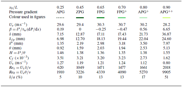
 δfp
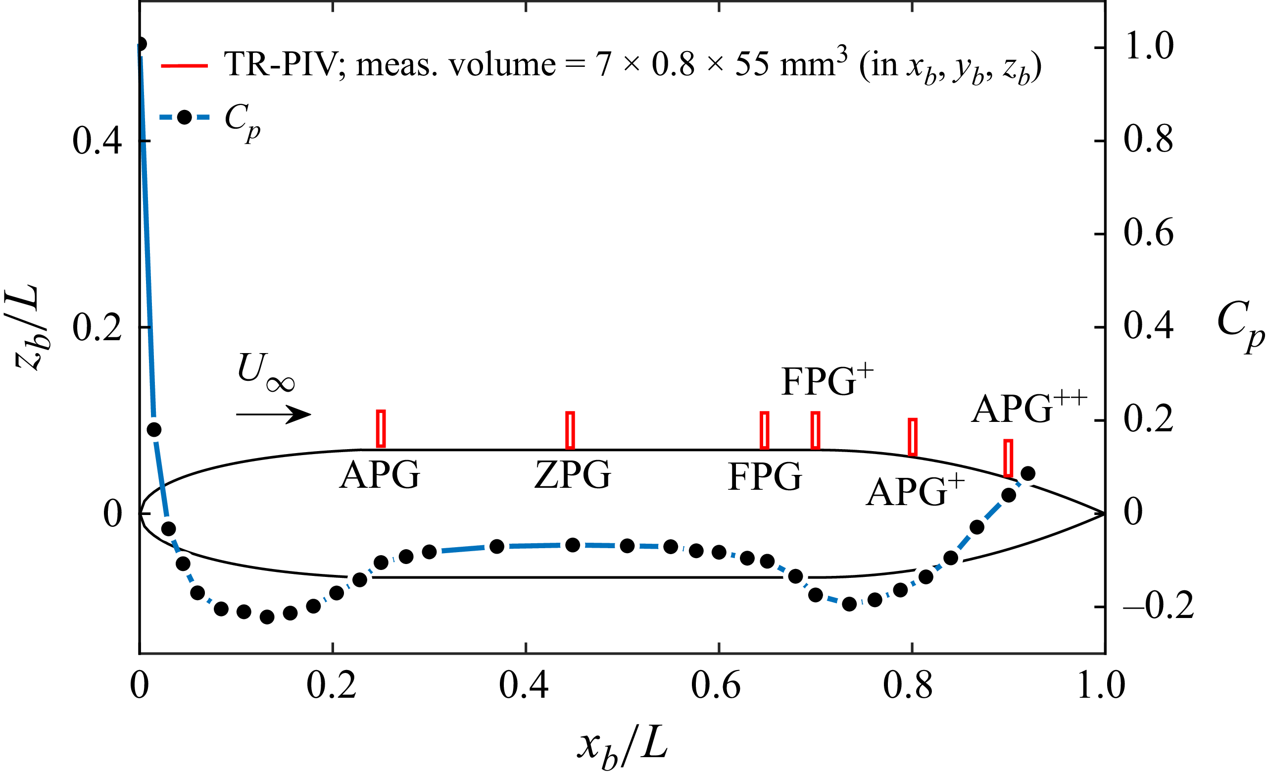
 xb
 zb
 Cp
 U∞
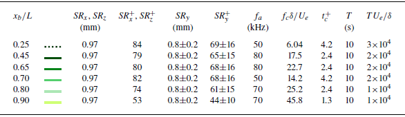
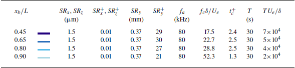

 ψ
 xb/L=0.80
 xb/L=0.90
 δ
 xb/L=0.90
 αx
 ∘
 xb
 zb
 x−z
 (xs,zs)
 ψ
 UUW
 Ub,Wb
 U,W

 U
 u2

 uiuwb
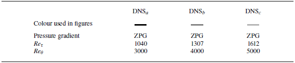

 δ
 δfp

 fΦuu/Ue2
 f′=fδ/Ue
 z≈0.2δ
 z≈0.5δ

 fΦuu/Ue2
 f″=fδfp/Ue
 δfp
 z≈0.2δ
 z≈0.5δ

 xb/L=0.45
 fΦuu/Ue2
 f″=fδfp/Ue
 t+
 −1
 −3
 fc′
 f2×IW′

 χ
 xb/L=0.45
 zr/δ=0.2
 zr/δ=0.5
 f″=fδfp/Ue
 t+
 γ2
 fΦuu/Ue2
 −1
 −3
 f2×IW′

 χ
 zr≈0.2δ
 0.5δ
 f″≈0.3
 f″≈0.1
 +ψ

 Ruu
 δ
 zr/δ=0.2
 0.5
 xb/L=0.45
 0.65
 0.80
 0.90
 xb/L
 0.90
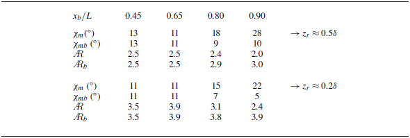
 χm
 AR
 Ruu
 zr/δ=0.5
 0.2
 xb/L
 χmb
 ARb
 ±2∘

 xb/L=0.45
 Θ
 Δx/δ
 f′=fδ/Ue=0.432±0.022(1000±50
 z+≈207
 0.20δ
 Rfit2
 Uc
 U
 Uc
 U
 fδ/Ue
 t+

 xb/L=0.45
 Uc/U
 f″=fδfp/Ue
 t+
 fΦuu/Ue2
 −1
 −3
 fc′
 f2×IW′

 δ
 δfp
 zr/δ=0.2,0.5
 0.8
 Ruu=0.3
 Λx
 δfp
 Uc/U
 f″≈0.3

 uiuwb
 u
 zwb


 Open access

