2. Preliminaries

Before presenting the proposed algorithm in detail, it is necessary to introduce three key concepts: the 4W4S kinematic model, the representation of Euclidean Signed Distance Field (ESDF) in path planning, and Douglas–Peucker (DP) algorithm for path post-processing.

2.1. 4W4S robotic model

For a robot with four-wheel independent steering configuration, directly modeling individual wheel steering angles increases the complexity of path planning. Therefore, an equivalent Ackermann-based kinematic model is adopted to describe the motion of the robot reference point:

(1) \begin{equation} \left[\begin{array}{l} {\, \dot{\kern-1.5pt{x}}}\\ \dot{y}\\ \dot{\theta }\\ \dot{\delta } \end{array}\right]=\left[\begin{array}{l} \cos (\theta )\\ \sin (\theta )\\[1pt] \dfrac{\tan (\delta )}{l}\\ 0 \end{array}\right]v+\left[\begin{array}{c} 0\\ 0\\ 0\\ 1 \end{array}\right]\omega \end{equation}

where x and y represent the robot’s position coordinates in the 2D plane, θ denotes the heading angle, $ \delta $ is the front wheel steering angle, l refers to the wheelbase between the front and rear axles, and v and $ \omega $ denote the linear and angular velocities of the robot, respectively.

The Ackermann steering model is illustrated in Figure 1. Given the vehicle’s wheelbase l and the maximum front wheel steering angle $ {\delta}_{max} $ , the minimum turning radius of the robot can be calculated as:

Figure 1.

Ackermann steering model and pivot-turning model.

(2) \begin{equation} R_{\min }=\frac{l}{{\tan}(\delta _{\max })} \end{equation}

To ensure complete turning behavior and smooth motion continuity, when the steering angle computed by the Ackermann model exceeds the maximum allowable steering angle, the robot temporarily switches to a pivot-turning model, as illustrated in Figure 1. In narrow environments, the zero-turn mode is activated when the Ackermann path cannot satisfy the minimum turning-radius constraint without collision, allowing the robot to rotate around its geometric centre. During mode transition, translational motion is stopped, after which the steering wheels are synchronously adjusted to the zero-turn configuration only when sufficient clearance is available. Once the heading adjustment is completed, the robot returns to the dual-Ackermann mode for continuous motion, avoiding repeated switching caused by a single steering-angle threshold. This dual-mode switching strategy ensures both the safety and maneuverability of the robot’s navigation.

2.2. ESDF map

The ESDF is a map representation widely used in robotic navigation. Unlike traditional occupancy grid maps, the ESDF assigns a value to each point, representing its signed Euclidean distance to the nearest obstacle. A positive value indicates that the point is outside the nearest obstacle, while a negative value means it is inside.

In a two-dimensional space, the signed distance assigned to point p is

(3) \begin{equation} d(\, p)=sign(\, p)\cdot \min _{q\in O}{\parallel p-q\parallel} \end{equation}

where O represents the set of obstacle points, and $\parallel p-q\parallel $ is the Euclidean distance between point p and obstacle point q. To account for the physical dimensions of the robot, the ESDF is constructed based on the inflated occupancy map rather than the original obstacle cells. The inflation radius is selected according to the robot footprint, so that the distance evaluation implicitly considers the body clearance of the robot.

In this study, the ESDF is used for global path planning based on a static occupancy map. It is employed to evaluate the geometric relationship between the planned path and static obstacles, rather than to model moving obstacles or perform dynamic collision avoidance.

2.3. Douglas–Peucker

The DP algorithm is a path simplification technique designed to reduce the number of points in a path while preserving its overall shape. By iteratively removing redundant points in robotic trajectory, the DP algorithm simplifies the path and improves computational efficiency.

For any segment connecting the start point pi and the end point pj, the algorithm calculates the perpendicular distance d from each intermediate point pk to the line between pi and pj. The formula for computing this distance is

(4) \begin{equation} d(\, p_{k})=\frac{| (x_{j}-x_{i})(y_{i}-y_{k})-(x_{i}-x_{k})(y_{j}-y_{i})| }{\sqrt{(x_{j}-x_{i})^{2}+(y_{j}-y_{i})^{2}}} \end{equation}

If the calculated distance is smaller than a predefined threshold, the intermediate point P _k is removed.

3. Algorithm description

To provide a unified formulation of the path-planning problem, this study aims to generate a feasible global path for the 4W4S robot that jointly considers path compactness, obstacle clearance, and kinematic feasibility. Specifically, the planned path is expected to remain relatively short while ensuring sufficient clearance from obstacles and satisfies the motion characteristics of the 4W4S robot, particularly the minimum turning-radius constraint under the dual-Ackermann steering mode. When Ackermann steering becomes infeasible in confined spaces, zero-turn mode is employed. Accordingly, the overall path-planning problem is formulated as follows:

(5) \begin{align} \min _{P} J(P)&=w_{\mathbf{1}}L(P)+w_{\mathbf{2}}C_{\mathrm{obs}}(P)\nonumber\\[-5pt] \text{ s}.\mathrm{t}.P(\mathbf{0})&=X_{\text{start}}, {\enspace}P(N)=X_{\text{goal}} \nonumber\\ d(P,O) &\geq d_{\text{safe}}, \\ R(P) &\geq R_{\min }, \nonumber \\ m&\in \{\text{Ackermann},\text{zero-turn}\} \nonumber \end{align}

where P denotes the planned path, L(P) is the path-length term, C _obs(P) represents the obstacle-related cost, d(P,O) denotes the clearance between the path and obstacles, d _safe is the prescribed safety distance, R(P) denotes the local turning radius, R _min is the minimum turning radius of the 4W4S robot, and m represents the motion mode, including dual-Ackermann steering and zero-turn rotation.

Unlike conventional planners that terminate once a collision-free geometric path is obtained, the proposed method further incorporates the steering feasibility of the 4W4S robot into path refinement. The key contribution is the integration of minimum-turning-radius correction and motion-mode adaptation: feasible turns are reconstructed using straight–arc connections under dual-Ackermann motion, while zero-turn motion is allowed only when no collision-free path satisfying the minimum turning-radius constraint can be found. The subsequent path-processing and trajectory-refinement procedures support this strategy by improving obstacle clearance and trajectory continuity.

3.1. Overall framework of the algorithm

This study proposes a path planning algorithm based on the kinematic model of a 4W4S robot, aiming to improve the feasibility of trajectories during turning maneuvers. When a turning action is required, the algorithm generates an arc-shaped path based on minimum turning radius, improving path validity and motion smoothness.

The proposed framework is constructed based on the successive requirements of path planning and execution for 4W4S robots. The sampling-based planner first provides a collision-free global path, followed by an obstacle-aware DP procedure that removes redundant waypoints without sacrificing collision avoidance. The minimum-turning-radius optimization then corrects geometrically sharp turns to satisfy the steering constraint of the robot. When this constraint cannot be satisfied in confined spaces, the zero-turn mode is introduced to expand maneuverability. Finally, polynomial trajectory optimization improves the continuity of the resulting trajectory for subsequent path tracking. Through this sequential design, the framework achieves progressive refinement.

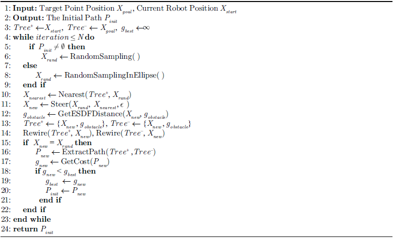
Algorithm 1 presents the overall procedure of the proposed method. Given the robot’s current position X _start and target point X _goal , an initial path P _init is first generated using a sampling-based algorithm. This path is then simplified by removing redundant points. Next, path optimization is performed based on the robot’s minimum turning radius and the simplified path. Finally, trajectory is further optimized under velocity and acceleration constraints to generate the final path P.

Algorithm 1.

Path optimization Method Based On The 4W4S Model

3.2. Initial path generation

In the initial path generation stage, RRT-Connect is employed to quickly produce an initial solution, which is then refined by Informed-RRT^* within an ellipsoidal domain using the initial path length as the constraint.

The traditional Informed-RRT^* algorithm focuses solely on minimizing path, which risks the robot colliding with obstacles. Although introducing an obstacle inflation layer such as Voronoi-based method enhances safety, it reduces the robot’s traversability in confined environments and results in a longer path length. To balance the trade-off between path length and safety, this study introduces a safety distance factor into the path cost function. This allows the optimization process to explicitly account for robot’s proximity to obstacles while minimizing path length. The proposed path cost is expressed as:

(6) \begin{equation} g=\alpha \cdot g_{\textit{length}}+\beta \cdot g_{\textit{obstacle}} \end{equation}

(7) \begin{equation} g_{\textit{obstacle}}=d_{safe}-d_{\textit{obstacle}} \end{equation}

where $ \alpha$ and $ \beta $ are user-defined cost weights, g _length and g _obstacle represent the cost terms for path length and obstacle clearance, respectively, d _safe denotes the predefined safety distance, and d _obstacle is the distance between a path point and the nearest obstacle. The two cost terms are combined through weighted summation, where $ \alpha$ and $ \beta $ determine the trade-off between path efficiency and obstacle avoidance. A larger obstacle clearance results in a lower obstacle-related cost, promoting safer path generation while maintaining path compactness.

During the sampling process, the distance between each sampled point and the nearest obstacle from the ESDF map are used and for computing the obstacle-related cost. Algorithm 2 presents the procedure for generating the initial path based on these sampled distances corresponding to the first step of Algorithm 1. Given the robot’s current position and the target point, the algorithm generates a feasible initial path that jointly considers path length and obstacle proximity.

Algorithm 2.

Get Initial Path

Algorithm 3.

Redundancy Removal

3.3. Redundancy removal

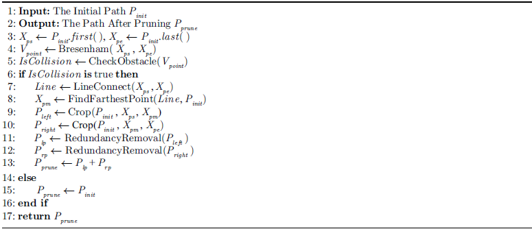
The initial path generated by the sampling algorithm often contains redundant points having little impact on the path shape or even interfering with subsequent optimization. The DP algorithm removes the redundant points to simplify the path by evaluating the shortest distance between a path point and the corresponding path segment. However, the standard DP algorithm relies solely on a distance threshold, making it prone to producing unsafe paths when obstacles are present. To address this, we enhance the DP algorithm by integrating an obstacle-checking mechanism, as shown in Algorithm 3. Specifically, the algorithm employs Bresenham’s line algorithm to retrieve all points along the line connecting two path nodes. Before removing any intermediate point, it performs a collision check with obstacles, thereby improving the algorithm’s efficiency and robustness. The occupancy map is inflated according to the robot footprint and used for collision checking.

Specifically, FindFarthestPoint(Line,P) searches within path for the point that has the maximum perpendicular distance from the line segment Line. Crop(P,X1,X2) extracts the segment of path P that starts from point X1 and ends at point X2.

Algorithm 4.

Path Optimization

Figure 2.

The process of path optimization.

3.4. Path optimization

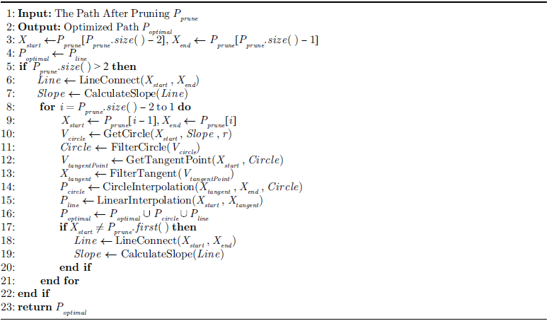
The core of the proposed algorithm lies in path optimization based on the robot’s minimum turning radius. A purely geometric approach is adopted to generate arc-shaped trajectories locally where turning is required. Algorithm 4 summarizes the overall process of path optimization.

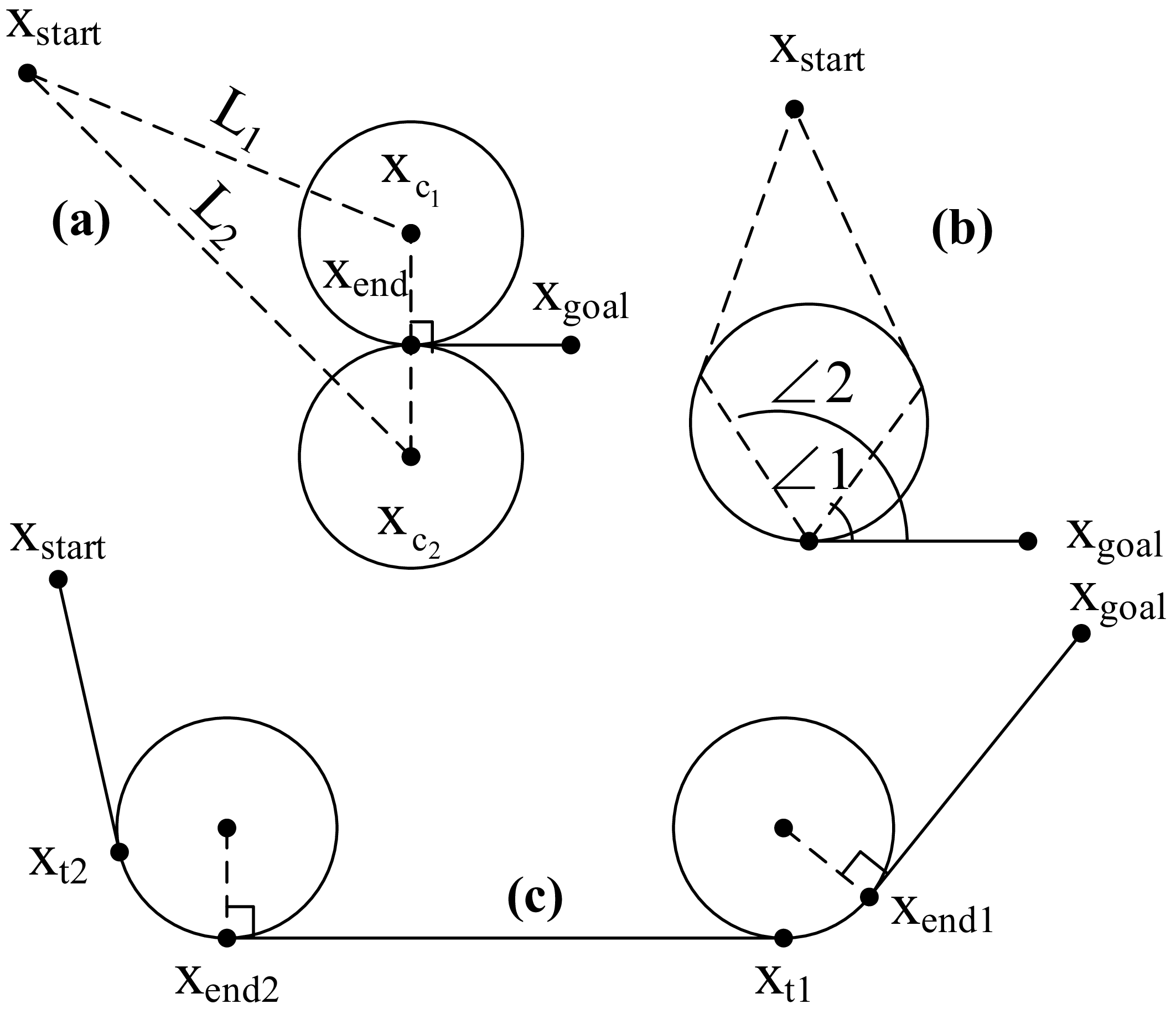
Specifically, GetCircle(X,Slope,r) uses point X as the base and r as the radius and calculates the coordinates of the circle center using the slope perpendicular to segment Slope. Two circle center solutions can be found, thereby two candidate circle equations are returned. FilterCircle(V _circle ) selects the circle whose center is closer to point X _start , as shown in Figure 2a. Since condition ∠1 $ \lt$ ∠2 holds, the circle centered at point X _c1X is retained. GetTangentPoint(X,Circle) computes the tangent points X from point to Circle. Since there are two tangents from a point to a circle, the function returns two tangent line equations. FilterTangent(V _tangent ) selects the tangent point that forms a larger angle with point X _end from the two candidates, as illustrated in Figure 2b. Since condition ∠1 $ \lt$ ∠2 is satisfied, the tangent point X _t2 is retained. CircleInterpolation(X ₁ ,X ₂ ,Circle) extracts the arc segment on Circle from point X ₁ to point X ₂ and performs path point interpolation along the arc. LinearInterpolation(X ₁ ,X ₂ ) performs path point X ₁ interpolation along the straight line from point to point X _2. The tangent point is selected to ensure a smooth connection between the straight segment and the circular arc, maintaining heading continuity. In addition, the radius of the selected arc is constrained to be no smaller than the robot’s minimum turning radius, ensuring steering feasibility.

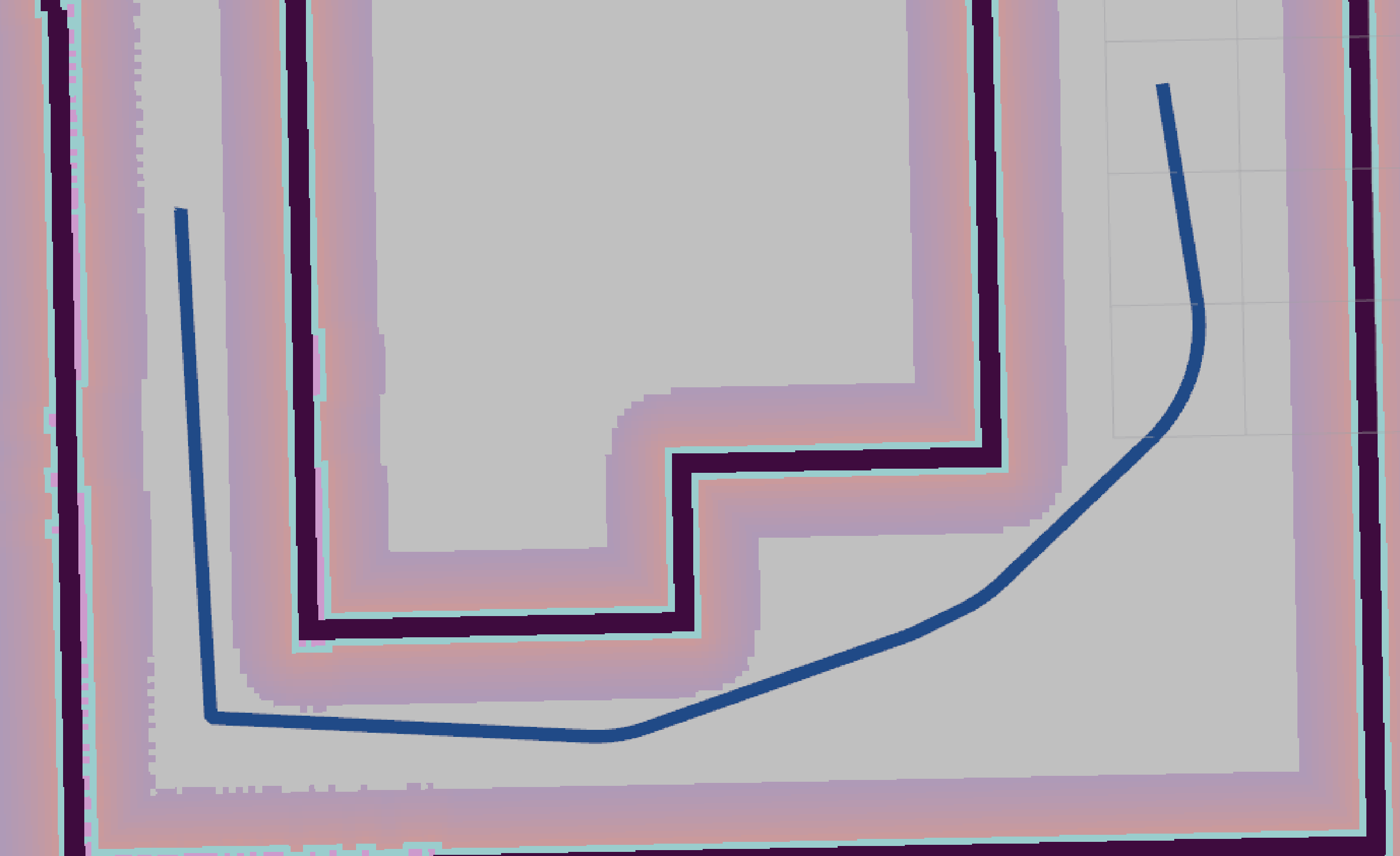
The path optimization method proposed in this study performs reverse optimization from the goal point back toward the starting point. Except for the segment between the goal and the second-to-last path point, which is connected by a straight line, all other adjacent path points are connected using a combination of straight lines and circular arcs, as illustrated in Figure 2c. The initial turning radius of the arc is user-defined and dynamically adjusted during execution. If the arc generated with the current radius collides with obstacles, the optimization is considered invalid, and the algorithm attempts to reduce the turning radius and replans. If the radius reaches the robot’s minimum turning radius yet collision still occurs, the arc-based optimization is abandoned, and a straight connection line is used instead. An initial value of two times of the minimum turning radius is recommended, though it can be adjusted to a user-specified value. An excessively large initial turning radius may cause invalid iterations in narrow spaces, increasing the algorithm’s runtime. As shown in Figure 3, if the left-side space is too narrow to satisfy the minimum turning radius, the optimization is skipped. This method is particularly effective in narrow environments, where Ackermann steering model may introduce high collision risks. Under such conditions, the system automatically switches to the 4W4S model, allowing the robot to pivot in to execute the turning maneuver safely.

Figure 3.

Path optimization strategy in narrow space.

3.5. Trajectory optimization

The optimized path fully accounts for the robot’s motion constraints, particularly the minimum turning radius. However, in practical applications, if the robot executes a sharp turn at the minimum radius, velocity, and acceleration constraints may be violated. This could result in degraded path tracking performance or even collisions. To enhance the executability of the path, this study adopts a polynomial interpolation approach to ensure continuity in position, velocity, and acceleration. This method generates smooth trajectories with continuous position, velocity, and acceleration profiles, thereby improving trajectory executability and reducing abrupt motion during path tracking.

If the trajectory is required to pass through two path points X(0) and X(t ₀) within a specified time interval t ₀, and the velocity constraints at the start and end points are given by $\,\dot{\!X}$ (0) and $\,\dot{\!X}$ (t ₀), along with acceleration constraints $\,\ddot{\!X}$ (0) and $\,\ddot{\!X}$ (t ₀), with a total of six degrees of freedom, the trajectory can be fully determined using a fifth-order polynomial:

(8) \begin{equation} X(t)=\boldsymbol{a}_{0}+\boldsymbol{a}_{1}t+\boldsymbol{a}_{2}t^{2}+\boldsymbol{a}_{3}t^{3}+\boldsymbol{a}_{4}t^{4}+\boldsymbol{a}_{5}t^{5} \end{equation}

where the polynomial coefficients are determined by the constraints on position, velocity, and acceleration:

(9) \begin{equation} \left[\begin{array}{l} \boldsymbol{a}_{0}\\ \boldsymbol{a}_{1}\\ \boldsymbol{a}_{2}\\ \boldsymbol{a}_{3}\\ \boldsymbol{a}_{4}\\ \boldsymbol{a}_{5} \end{array}\right]=\left[\begin{array}{l} \boldsymbol{X}(0)\\ {\, \dot {\boldsymbol{\kern-2pt {X}}}}(0)\\ \dfrac{1}{2}{\, \ddot{\boldsymbol{\kern-1.5pt{X}}}}(0)\\[8pt] \dfrac{10}{{t}_{0}^{3}}[\boldsymbol{X}\left(t_{0}\right)-\boldsymbol{X}(0)]-\dfrac{1}{{t}_{0}^{2}}[4{\, \dot {\boldsymbol{\kern-2pt {X}}}}\left(t_{0}\right)+6{\, \dot {\boldsymbol{\kern-2pt {X}}}}(0)]+\dfrac{1}{2t_{0}}[{\, \ddot{\boldsymbol{\kern-1.5pt{X}}}}\left(t_{0}\right)-3{\, \ddot{\boldsymbol{\kern-1.5pt{X}}}}(0)]\\[5pt] \dfrac{-15}{{t}_{0}^{4}}[\boldsymbol{X}\left(t_{0}\right)-\boldsymbol{X}(0)]+\dfrac{1}{{t}_{0}^{3}}[7{\, \dot {\boldsymbol{\kern-2pt {X}}}}\left(t_{0}\right)+8{\, \dot {\boldsymbol{\kern-2pt {X}}}}(0)]-\dfrac{1}{2{t}_{0}^{2}}[2{\, \ddot{\boldsymbol{\kern-1.5pt{X}}}}\left(t_{0}\right)-3{\, \ddot{\boldsymbol{\kern-1.5pt{X}}}}(0)]\\[5pt] \dfrac{6}{{t}_{0}^{5}}[\boldsymbol{X}\left(t_{0}\right)-\boldsymbol{X}(0)]-\dfrac{1}{{t}_{0}^{4}}[3{\, \dot {\boldsymbol{\kern-2pt {X}}}}\left(t_{0}\right)+3{\, \dot {\boldsymbol{\kern-2pt {X}}}}(0)]+\dfrac{1}{2{t}_{0}^{3}}[{\, \ddot{\boldsymbol{\kern-1.5pt{X}}}}\left(t_{0}\right)-{\, \ddot{\boldsymbol{\kern-1.5pt{X}}}}(0)] \end{array}\right] \end{equation}

By computing the polynomial coefficients from the specified boundary conditions, the proposed method ensures continuous position, velocity, and acceleration along the trajectory.

4. Simulations in Gazebo

To comprehensively evaluate the performance of the proposed algorithm, we conducted experiments in simulation environment.

As shown in Figure 4, the simulation environment was constructed in Gazebo to emulate a typical warehouse scenario. In the map, four points, A, B, C, and D, were selected as navigation goals. The algorithm was implemented on Ubuntu 20.04 with ROS Noetic. It relies on the move-base navigation framework and uses the Cartographer [Reference Hess, Kohler, Rapp and Stewe26] to provide grid maps and real-time localization information. The inflation radius of the cost map in move-base was set to 0.5 m. To evaluate kinematic feasibility, the robot in Figure 4 was configured with a maximum steering angle of 15 degree, a minimum turning radius of 0.5 m, and an initial turning radius of 1 m. The number of sampling iterations was set to 1,500. The cost weight of path length was 1, while the cost weight of obstacle clearance was 5, with predefined safety distance of 1 m.

Figure 4.

Simulation environment and model.

Figure 5.

Visualization of the path at each stage.

As shown in Figure 5, the proposed planner follows a multi-stage refinement process consisting of initial path generation, redundancy removal, path optimization, and trajectory optimization. In the initial stage, RRT-Connect rapidly generates a feasible path, which is further refined by Informed-RRT^* within the informed sampling region. The obstacle-aware DP algorithm then removes redundant waypoints while preserving collision-free connectivity, resulting in a more concise path that retains its original topology. Subsequently, the minimum-turning-radius optimization replaces sharp and kinematically infeasible turns with straight–arc connections under the turning-radius constraint, particularly in open environments such as goals A and B. In narrow regions (goals C and D), the improvement is limited due to spatial constraints. Finally, polynomial trajectory optimization further enhances local trajectory continuity. As shown in Figure 6, the average point displacements after trajectory optimization are only 0.005 m and 0.004 m for goals A and B, respectively, while the curvature profiles exhibit reduced local abruptness and smoother transitions. These stage-wise results demonstrate the distinct contributions of the individual components to path refinement and trajectory executability.

Figure 6.

Trajectory optimization results.

Figure 6. Long description

Panel A: A scatter plot titled ‘Path Point Distance Difference to Goal A’ shows Euclidean Distance (m) on the y-axis and Point Index on the x-axis. Data points are color-coded from blue to red, indicating varying distances. A dashed line represents the average distance of 0.005 meters. Panel B: A line graph titled ‘Path Curvature to Goal A’ displays Curvature (m^-1) on the y-axis and Point Index on the x-axis. Two lines, one blue for post-trajectory planning and one orange for pre-trajectory planning, show curvature trends. Panel C: A scatter plot titled ‘Path Point Distance Difference to Goal B’ shows Euclidean Distance (m) on the y-axis and Point Index on the x-axis. Data points are color-coded similarly to Panel A, with a dashed line indicating an average distance of 0.004 meters. Panel D: A line graph titled ‘Path Curvature to Goal B’ displays Curvature (m^-1) on the y-axis and Point Index on the x-axis. Two lines, one blue for post-trajectory planning and one orange for pre-trajectory planning, show curvature trends.

Table I.

Performance of algorithms in simulations.

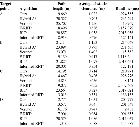
Table I. Long description

A table comparing the performance of different algorithms in simulations. The table has four rows and six columns. The columns are labeled Target point, Algorithm, Path length (m), Average obstacle clearance (m), and Runtime (ms). The row labels are A, B, C, and D. Each row provides data for different algorithms: Ours, Hybrid A*, Voronoi, F-RRT*, BIT*, and Informed RRT*. For target point A, the path lengths range from 18.496 to 25.707 meters, average obstacle clearances range from 0.676 to 1.256 meters, and runtimes range from 19.769 to 3,157.379 milliseconds. For target point B, the path lengths range from 19.139 to 23.894 meters, average obstacle clearances range from 0.795 to 1.402 meters, and runtimes range from 15.562 to 2,013.651 milliseconds. For target point C, the path lengths range from 13.013 to 23.56 meters, average obstacle clearances range from 0.426 to 0.827 meters, and runtimes range from 8.121 to 2,309.407 milliseconds. For target point D, the path lengths range from 11.348 to 20.573 meters, average obstacle clearances range from 0.588 to 1.086 meters, and runtimes range from 9.488 to 2,014.057 milliseconds.

Table I and Figure 7 compare the proposed method with Hybrid A^*, Voronoi, F-RRT^* [Reference Liao, Wan, Hua, Ma, Zhu and Qing27], Informed RRT^* [Reference Gammell, Srinivasa and Barfoot28], and BIT^* [Reference Gammell, Srinivasa and Barfoot29] in terms of path quality, obstacle clearance, and planning efficiency. Overall, the proposed method achieves a favorable balance among path compactness, safety clearance, and execution feasibility for 4W4S robot navigation.

Figure 7.

Path comparison in simulation environment.

Figure 7. Long description

The image contains seven separate diagrams comparing different path planning algorithms for a robot in a simulated environment. Each diagram shows the robot’s path through a complex layout of obstacles. The diagrams are labeled as Ours, Hybrid A*, Voronoi, F-RRT*, BIT*, and Informed RRT*. Each path is depicted with different colored lines, indicating the trajectory taken by the robot using each algorithm. The diagrams illustrate how each algorithm navigates the robot through the environment, highlighting differences in path efficiency, smoothness, and obstacle avoidance.

Table II.

Statistical reliability evaluation of sampling-based planners.

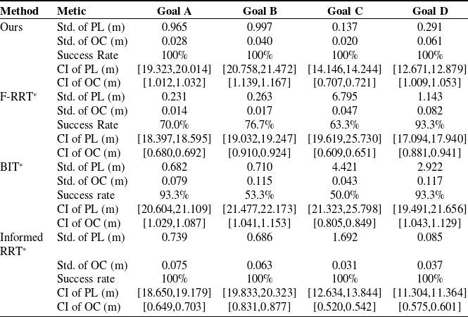
Table II. Long description

The table presents a statistical reliability evaluation of sampling-based planners, comparing five methods across four goals. The methods evaluated are Ours, F-RRT*, BIT*, and Informed RRT*. The metrics used for evaluation include the standard deviation of path length (Std. of PL) in meters, standard deviation of obstacle clearance (Std. of OC) in meters, success rate in percent, confidence interval of path length (CI of PL) in meters, and confidence interval of obstacle clearance (CI of OC) in meters. The table has five rows for each method and five columns for each metric. Each row provides specific values for the respective method and goal. For example, for Goal A, the method Ours has a Std. of PL of 0.965 meters, a Std. of OC of 0.028 meters, a success rate of 100 percent, a CI of PL of [19.323, 20.014] meters, and a CI of OC of [1.012, 1.032] meters. Similar detailed values are provided for other methods and goals.

The proposed method does not always generate the shortest path, since Informed RRT^* obtains shorter trajectories in some scenarios due to its efficient informed sampling strategy. However, path length alone is inadequate for 4W4S robots, which require consideration of both obstacle avoidance and kinematic constraints. By incorporating obstacle-aware refinement, minimum turning-radius optimization, and motion-mode adaptation, the proposed method generates paths with competitive compactness and improved kinematic feasibility.

Regarding obstacle clearance, the proposed method achieves an average clearance of approximately 1.00 m, which is higher than Hybrid A^*, F-RRT^*, and Informed RRT^*, while slightly lower than Voronoi and BIT^*. The larger clearance of Voronoi and BIT^* is mainly attributed to their tendency to generate paths farther from obstacles, but often at the cost of longer detours. The proposed method therefore provides a better balance between safety margin and path efficiency.

For planning efficiency, the proposed method achieves an average runtime of approximately 221 ms. Although slower than Informed RRT^* and Voronoi, it remains faster than F-RRT^* and BIT^*. The additional computational cost mainly results from the path refinement and kinematic optimization procedures required for 4W4S execution. Moreover, runtime comparisons among different planners should be interpreted considering their different planning mechanisms, since Hybrid A^* performs deterministic search in discretized state spaces, whereas RRT^*-based methods explore continuous spaces through stochastic sampling. Therefore, Table I provides an empirical comparison under identical experimental conditions rather than an absolute ranking of computational efficiency.

Since sampling-based planners are affected by randomness, 30 independent trials were further conducted for Ours, F-RRT^*, Informed RRT^*, and BIT^*. The statistical results are summarized in Table II. In this table, Std. represents the standard deviation, CI represents the confidence interval, PL represents path length, and OC represents obstacle clearance. The proposed method achieves a 100% success rate across all scenarios and exhibits lower variability in both path length and obstacle clearance. Particularly in the constrained Goal C environment, the proposed method obtains a path-length standard deviation of only 0.137 m with a narrow 95% confidence interval, while F-RRT^* and BIT^* exhibit significantly larger variations and lower success rates. These results demonstrate that the proposed framework provides more reliable and repeatable planning performance under stochastic sampling conditions.

Overall, the proposed method does not simply optimize path length, but achieves a comprehensive balance among path quality, obstacle clearance, statistical reliability, and 4W4S-specific robot execution requirements.

The wheel-speed curves (Figure 8) provide additional evidence from the execution perspective. For both the left and right front wheels, the proposed method generally exhibits fewer prolonged low-speed intervals and less scattered speed fluctuation during tracking. In cases A and B, Voronoi and F-RRT^* show longer execution windows and more repeated speed drops, consistent with their longer or less trackable paths. Hybrid A^* presents frequent speed reductions in local turnings, caused by the piecewise and obstacle-hugging path shape. By comparison, the wheel-speed profiles of the proposed method are more concentrated around the cruising speed with abrupt deceleration segments, indicating less severe local correction during tracking. This is consistent with the shorter average path length and smoother geometric path observed above.

The steering-angle curves (Figure 9) reveal an even more important difference in tracking behavior. In this work, when the absolute value of the wheel steering angle reaches 0.900825 rad, the vehicle switches to the zero-turn mode. It should be noted that zero-turn events at the beginning are expected due to initial heading misalignment; therefore, subsequent occurrences are more indicative of path quality. The proposed method generally requires fewer and shorter additional zero-turn intervals than Voronoi and F-RRT^*. In trajectory to A, Voronoi exhibits a clear mid-course zero-turn event, indicating an excessive heading correction too large to be handled by the steering mode alone. In Scenario B, F-RRT^* shows obvious zero-turn in the middle of the run, suggesting locally aggressive turning demands. In trajectory to D, Voronoi and F-RRT^* both present multiple zero-turn events beyond the initial stage, while the proposed method avoids such repeated switching. Trajectory to C is particularly noteworthy for the safety concern: a mid-course zero-turn is observed for the proposed method, which aligns with the narrow-passage strategy, allowing necessary mode switching instead of enforcing overly strict curvature smoothing.

Overall, the comparison demonstrates that the proposed method is not only competitive in conventional planning metrics but also more favorable in downstream tracking performance. Compared with Hybrid A^*, Voronoi, and F-RRT^*, it maintains competitive path lengths while providing sufficient obstacle clearance and smoother wheel-speed and steering-angle profiles during execution. Moreover, the zero-turn events are trigged by actual spatial constraints rather than geometric irregularities. This indicates that the proposed planner is more suitable for practical navigation of 4W4S robots in cluttered and narrow construction environments, where path quality and motion executability must be considered jointly.

5. Experiments in real world

In the real-world experiments, we employed a 4W4S robotic platform with a length of 1.78 m and a width of 1.2 m, as illustrated in Figure 10. The 4W4S mobile robot was developed for navigation tasks in construction environments. It is equipped with eight motors, including four driving motors and four-steering motors, and all actuators are controlled through CAN communication. The software stack is built on Ubuntu 20.04 with ROS Noetic serving as the middleware. For perception, the robot is equipped with a Helios 32-channel LiDAR sensors for environmental mapping and obstacle detection, as well as a KY-IMU1714 inertial measurement unit to provide reliable motion state estimation. Each wheel is independently steerable. To improve maneuverability during turning, the robot adopts a dual-Ackermann steering mode during normal forward motion, in which the rear wheels steer at the same angle as the front wheels but in the opposite direction. In the dual-Ackermann steering mode, the maximum steering angle of each wheel is 30°. Given that the distance between the front and rear axles is 1.38 m. It should be noted that the minimum turning radius calculated in Eq. (2) is based on the conventional Ackermann steering model. In practice, the 4W4S robot adopts a dual-Ackermann configuration, where the rear wheels steer oppositely to the front ones, resulting in a smaller turning radius. Therefore, the effective minimum turning radius is approximately half of the value calculated by Eq. (2), i.e., 1.2 m for the proposed platform.

Figure 8.

Wheel speed comparison.

Figure 9.

Wheel steering angle comparison.

Figure 10.

Experimental robot and environment.

In the real-world experiments, the proposed method was compared with Hybrid A^*, Voronoi, and F-RRT^* in terms of path characteristics and steering behavior. In the experiments, the cost weight of path length was set to 1, and the cost weight of obstacle clearance was set to 10. In addition, the predefined safety distance was configured as 3 m, the number of samples for obtaining the initial path was set to 2,500, and the optimal turning radius of the robot was specified as 1.7 m.

Figure 11.

Map dimensionality reduction.

Figure 12.

Robot navigation process.

Figure 13.

Global path comparison.

Figure 13. Long description

Panel A: The path planning method labeled ‘Ours’ shows a blue path navigating around obstacles in a complex environment. The path appears smooth and efficient. Panel B: The path planning method labeled ‘Hybrid A*’ displays a blue path with more turns and less efficiency compared to ‘Ours’. Panel C: The path planning method labeled ‘Voronoi’ shows a blue path that is less smooth and more convoluted than the path in ‘Ours’. Panel D: The path planning method labeled ‘F-RRT*’ presents a blue path that is more direct but still less efficient than the path in ‘Ours’.

As shown in Figure 11, a 3D map of the experimental environment was previously constructed using LIO-SAM. The resulting PCD map was then projected into a 2D PGM map and used by the move_base framework. In addition, LiORF-Localization was employed to perform 3D localization based on the PCD map, providing real-time robot pose information for the navigation algorithm. The inflation radius in move_base was set to 1.1 m. The algorithm parameters were kept consistent with those used in the simulation. After the global path was planned, the robot tracked the path using the Pure Pursuit algorithm.

Figure 12 illustrates the process by which the robot moves from the start point to the goal point by tracking the global path generated by the proposed method. Meanwhile, tracking experiments were also conducted on the robot using the comparison algorithms. Figure 13 presents the global paths generated by the proposed method and the comparison algorithms. Overall, the proposed method produces a more compact and smoother path, with better continuity at corners and smaller heading variations during turning. Hybrid A^* can also generate a relatively short path, but its local turns are more abrupt, and the geometric transition at corners is unnatural. Voronoi maintains a relatively large average obstacle clearance, but lower path compactness caused by detours. Although F-RRT^* is able to generate a feasible path, but exhibits polyline-like turns and insufficient obstacle clearance. In comparison, the proposed method achieves a better balance among reachability, path compactness, smoothness, and average obstacle clearance, making it more suitable for subsequent real-world tracking and stable execution.

Figure 14 shows the real-time steering-angle profiles of the front wheels, while the robot tracks the global paths generated by different planners. In the experiments, a steering-angle magnitude approaching 1 indicates that the robot switches from the dual-Ackermann mode to the zero-turn mode, which compromises navigation fluency.

Figure 14.

Wheel steering angle comparison.

Figure 15.

Navigation in narrow areas.

Figure 16.

Wheel steering angles during path trackings.

Among all methods, the proposed planner exhibits the smoothest and most stable steering behavior. For both the left and right front wheels, the steering angles remain within a relatively small range during the tracking process, without prolonged interval close to ±1 being observed. This indicates that the global path generated by the proposed method can be mostly tracked under the dual-Ackermann mode, with very few switches to the zero-turn mode. It is consistent with the geometric characteristics of the planned path: the proposed method produces a smoother and more compact trajectory with fewer abrupt heading changes, thereby reducing the local steering demand during tracking and improving the overall fluency of real-vehicle navigation. In comparison, Hybrid A^* shows several sharp steering peaks in local turning sections, Voronoi presents the most frequent large-amplitude oscillations and repeated near-saturation intervals, and F-RRT^* contains noticeable local fluctuations. Overall, these results demonstrate that the proposed method is more favorable for practical execution, as it effectively reduces large steering corrections and unnecessary mode switching for the 4W4S robot.

We also experimentally validated the switch ability of the proposed method in narrow environments. Figure 15 illustrates the global path generated by the proposed method in a confined area, as well as the robot’s dual-mode switching behavior during path tracking. Figure 16 shows the steering-angle profiles of the front wheels. For most of the tracking process, the steering angles remain within a relatively small range, indicating smooth execution under the dual-Ackermann mode. Only one short interval exhibits a sharp steering when the narrow space is encountered. The angle magnitude approaches 1, indicating a switching to the zero-turn mode. After the interval, the steering angle quickly drops. This result shows that the proposed path-planning strategy can effectively switch only in narrow areas, thereby improving both safety and navigation fluency.