1. INTRODUCTION
In the field of maritime security, large amounts of data, especially from ships' AIS (automatic identification systems), are generated each day, all of which contain information mutually exchanged between ships as well as ship-to-shore communications. Ships at sea can obtain the navigation status of the surrounding ships through AIS. Meanwhile, the shore-based monitoring centre can also obtain dynamic and static information from all vessels equipped with AIS equipment. Consequently, the amount of information is increasingly overwhelming to human and machine operators (Zhang et al., Reference Zhang, Liu, Cai, Wu and Shi2016). The goal of this study is to improve the efficiency of maritime supervision systems by learning from the mass of AIS data and mining it for rules on the movement of ships. It is a challenge to excavate the sailing features of ships from these data and to improve the efficiency of maritime supervision system with these features.
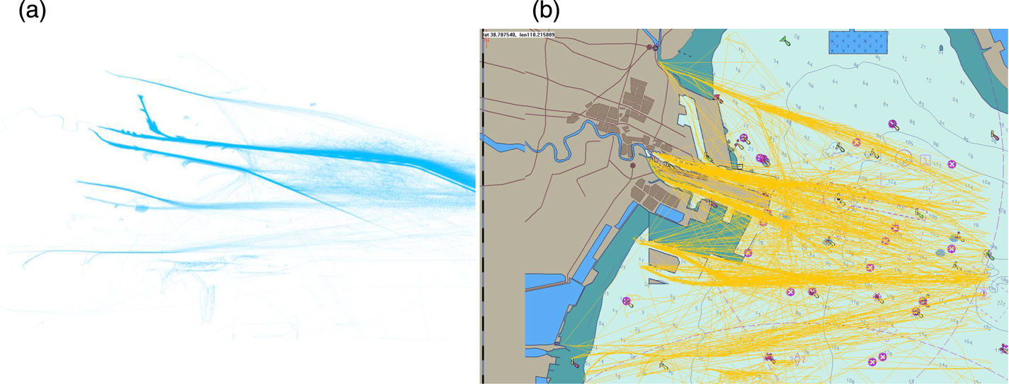
Ships equipped with ship-borne AIS send their own motion state to the shore-based management centre from time to time, from which a large number of tracks are displayed on electronic charts (as shown in Figure 1) to be seen visually. How to make good use of these data, however, is an issue that researchers are eager to solve. According to the literature (Lei, Reference Lei2016), the uncertainty of maritime trajectory data has increased the difficulty of studying the motion rules of ships. First, there is spatial uncertainty caused by the positioning accuracy of the ship-borne positioning equipment and calculation error, as well as the time uncertainty caused by different sampling rates and time lengths. Second, compared with trajectory data from road networks, ships are less constrained when navigating in the ocean. Ship navigation is usually affected only by water depth and obstacles, except in ports with traffic separation schemes, so ships' movements are relatively free (Lei, Reference Lei2016).
Each ship trajectory is composed of points in geographic space: (a) ship trajectories and the included position points; (b) ship trajectories superimposed on the electronic chart. It can be seen that the starting position or ending position of the trajectory is the berth in port, so that each can be classed as inbound or outbound trajectory. Electronic charts can more clearly represent the meaning of ship trajectories.

Increasing numbers of researchers are dedicated to research in intelligent maritime surveillance systems (Rhodes et al., Reference Rhodes, Bomberger, Seibert and Waxman2005; Laxhammar, Reference Laxhammar2008). The so-called intelligent maritime supervision means that the system can sense the situation in the entire jurisdiction sea area and analyse automatically the behaviour of a ship in the sea area, in order to give a report of the ship's motion status, which could provide the basis for decision-making by the relevant system while liberating the human operators from complicated tasks (Arguedas et al., Reference Arguedas, Pallotta and Vespe2017).
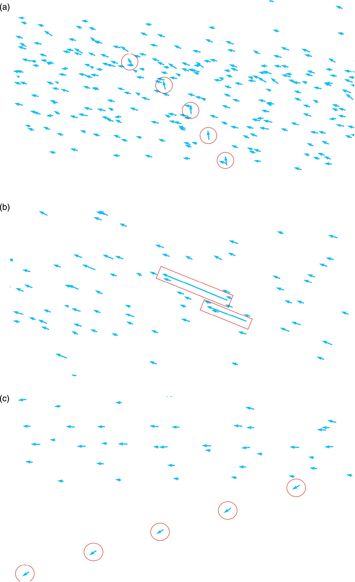
This paper studies the identification of abnormal behaviour of ships by an intelligent maritime supervision system. Davenport (Reference Davenport2008) divided abnormal motions of ships into 16 types, which has provided guidance to subsequent studies by the other scholars. In the present paper, three kinds of abnormal behaviours are identified: heading anomaly, speed anomaly and positional anomaly. Speed anomaly here includes both excessively fast and excessively slow speeds (as shown in Figure 2).
Examples of abnormal behaviours of ships: (a) heading anomaly, (b) speed anomaly, (c) positional anomaly.

In Figure 2(a), the arrow marked by the red circle indicates that the heading state is different from the heading distribution of the surrounding targets. The continuous state of the ship is observed. Here, the navigation behaviour can be defined as heading anomaly, i.e., heading across the channel. As can be seen in Figure 2(b), the target speed marked by the red rectangle is significantly higher than that of the surrounding targets. This behaviour is defined as speed anomaly. Figure 2(c) is a schematic diagram of the abnormal position of the ship, from which it can be seen that the target marked by the red circle deviates from the channel.
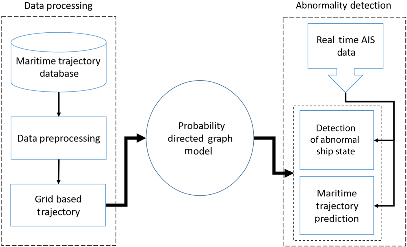
In this paper, the ship's trajectory is discretised into corresponding meshes based on mapped meshing and the grids are used as the node to establish a directed graph to obtain the state statistical characteristics of each node in the ship. With these statistical characteristics of each node, abnormal behaviour of the ship in future time can be detected. By calculating the probability of each directed edge, a probability directed graph is established to predict the normal trajectory of the ship at a future time; thereby it can be judged whether the ship has the potential to behave abnormally. In this essay, real AIS historical data from the port of Tianjin, China, is taken as the learning object to establish the probabilistic directed graph model. The workflow of the model is shown in Figure 3. The rest of this paper is organised as follows. Section 2 reviews related work. Section 3 illustrates the workflow of our model. In Section 4, we design the experiments and show the results. Finally, we draw conclusions and propose future works in Section 5.
Workflow chart of ship abnormal behaviour detection model based on probabilistic directed graph model.

2. RELATED WORK
Research on detection of anomalies in the maritime field began in the 1990s (Martineau and Roy, Reference Martineau and Roy2011) and has always been an active research field, arousing great interest from researchers. According to the types of abnormal behaviour of ships, maritime anomaly detection can be classified into five types of anomaly: location, context, motion, complex and data-related. Location anomaly means that the ship deviates from the normal channel or the normal area. Laxhammar et al. (Laxhammar, Reference Laxhammar2008; Laxhammar et al., Reference Laxhammar, Falkman and Sviestins2009; Rikard, Reference Rikard2010), taking advantage of the probability density function, obtained the statistical characteristics of four-dimensional feature space of ships (that is, the ship's latitude and longitude coordinates, and velocity distribution in the latitude and longitude directions). Mascaro et al. (Reference Mascaro, Nicholso and Korb2014) conducted detection of a variety of anomalies to identify fault data on land. Ristic et al. (Reference Ristic, La Scala, Morelande and Gordon2008) obtained the boundary of the trajectory pattern with kernel density estimation (KDE). If the ship sails outside the boundary, it is defined as location anomaly. Lei (Reference Lei2016) meshed the sea area, extracted trajectory frequent areas based on the given thresholds, and defined the location points outside the frequented areas as anomalies. Context anomaly means that the abnormal behaviour of the ship is directly related to the navigation environment. Hayes and Capretz (Reference Hayes and Capretz2015) discussed the relations between the abnormal behaviour of ships and time, such as seasons, holidays, etc. Movement anomaly refers to abnormality of the course and the speed of a ship, such as reverse navigating of the ship in the channel, U-turn, sudden stop and sudden steer (Laxhammar, Reference Laxhammar2008; Laxhammar et al., Reference Laxhammar, Falkman and Sviestins2009; Lei, Reference Lei2016). Complex anomaly refers to abnormal behaviours that could be detected with various anomaly detectors, such as drug smuggling, human smuggling, terrorism and other complex anomalous behaviours (Kowalska and Peel, Reference Kowalska and Peel2012). Pallotta et al. (Reference Pallotta, Vespe and Bryan2013) discussed anomalous ships in a wandering state, which relies on a speed-gating algorithm (comparing actual and estimated future displacement of ships). Data-related anomaly usually refers to incomplete trajectory data for a ship (Dobrkovic et al., Reference Dobrkovic, Iacob and van Hillegersberg2018).
Various methods are adopted by researchers to detect maritime anomalies, such as statistical (Johansson and Falkman, Reference Johansson and Falkman2007; Ristic et al., Reference Ristic, La Scala, Morelande and Gordon2008; Laxhammar et al., Reference Laxhammar, Falkman and Sviestins2009; Kowalska and Peel, Reference Kowalska and Peel2012; Mascaro et al., Reference Mascaro, Nicholso and Korb2014), clustering, neural network (Riveiro et al., Reference Riveiro, Johansson, Falkman and Ziemke2008) and graph (Johansson and Falkman, 2008; Mascaro et al., Reference Mascaro, Nicholso and Korb2014) based methods, and so on. In recent years, many new research results have emerged in this field. Zhao and Shi (Reference Zhao and Shi2019) designed a maritime anomaly detection model based on recurrent neural network and density-based clustering method. Varlamis et al. built a semantic network model and used a probability graph to analyse the abnormal trajectory of ships (Varlamis et al., Reference Varlamis, Tserpes, Etemad, Júnior and Matwin2019). Fahn et al. proposed a complete scheme for maritime surveillance using image sequences on embedded satellite systems, including maritime object detection, tracking and abnormal activity classification (Fahn et al., Reference Fahn, Ling, Yeh, Huang and Wu2019). Pitsikalis, in close collaboration with domain experts, developed a library of maritime patterns which can identify different kinds of ships, such as fishing boats, tugboats, etc. (Pitsikalis et al., Reference Pitsikalis, Artikis, Dreo, Ray, Camossi and Jousselme2019). Venskus extended the previous study on a self-organising map application for processing of sensor stream data received by the maritime AIS and improved the accuracy of the algorithm (Venskus et al., Reference Venskus, Treigys, Bernatavic̆ienė, Tamulevic̆ius and Medvedev2019).
In the field of maritime anomaly detection, whether it is based on statistical, clustering-based, neural network-based, or graph-based methods, all are categories of machine learning. The statistical-based method mainly uses the KDE or Gaussian Mixed Model (GMM) method to model the data, so as to obtain the probability distribution of the ship's trajectory points. The clustering-based method uses a clustering algorithm to classify ship trajectories, and trajectories with the same characteristics are divided into the same category. The method based on neural networks is to integrate the characteristics of trajectory into the network layers and control the output results by adjusting the weight matrix of the network. In contrast with these methods, the anomaly detection model based on the probability graph method is easier to understand and can more clearly represent the relationship between features. The model constructed in this paper is based on the probability graph and learns the ship history data, enabling it more intuitively to represent the ship trajectories.
The graph model-based method is a relatively new application method, which generates the traffic network graph with the trajectory nodes by considering the connectivity of the nodes in the network. The traffic is represented in a graph-based manner between predefined sets of nodes, while the network is a topology map derived as a node connection. Caschili et al. (Reference Caschili, Medda, Parola and Ferrari2014) analysed the trajectory through network representation and derived the main indicators of ship network connectivity based on the network representation. However, though this web-based representation is very useful to describe shipping activities, it has little capacity for classification and anomaly detection. Arguedas et al. (Reference Arguedas, Mazzarella and Vespe2015, Reference Arguedas, Pallotta and Vespe2017) put forward a representation method based on geographic network, deduced a simplified structural diagram of maritime activities, and gave some examples of anomaly detection. From the existing research results, it can be found that the graph model-based algorithm can establish a ship navigation network, but lacks in-depth analysis and detection of specific anomalous behaviours. According to previous studies and combining the anomaly detection algorithm based on grid partitioning and the graph model, a ship anomaly behaviour detection algorithm is put forward in this paper based on a probabilistic directed graph model, which discretises the ship state into corresponding grids to construct the probabilistic directed graph model. This model can analyse the state of the ship and predict the future normal trajectory of the ship to detect whether the behaviour of the ship is abnormal.
3. THE PROPOSED MODEL
This section introduces the ship anomaly behaviour detection model based on the proposed probability directed graph. As shown in Figure 3, the model includes three modules: data processing, model construction, and abnormal behaviour detection. The detailed operation process of these three modules will be discussed in the following subsections.
3.1. Data preprocessing
Definition 1: Original trajectory: An original AIS trajectory T is defined as T = {p i}, where p i = (loni, lati), i ∈ [1, n] and p i represents the ith position point of trajectory T. (loni, lati) stands for the geographic coordinates of the ship's current position. Finally, n is the length of trajectory T.
Data preprocessing is an important part of the data mining process, for it affects greatly the efficiency of data mining algorithm. Through analysis of the original AIS data, it is found that there is a large amount of fault data in the dataset, which can affect the accuracy of the anomaly detection algorithm. Moreover, because of the inherent characteristics of the data generation device, the obtained original trajectory data are of irregular time-series data. Therefore, it is necessary to process the raw data so as to improve the accuracy and integrity of the data. The preprocessing procedures applied to the original data proposed in this essay are as follows:
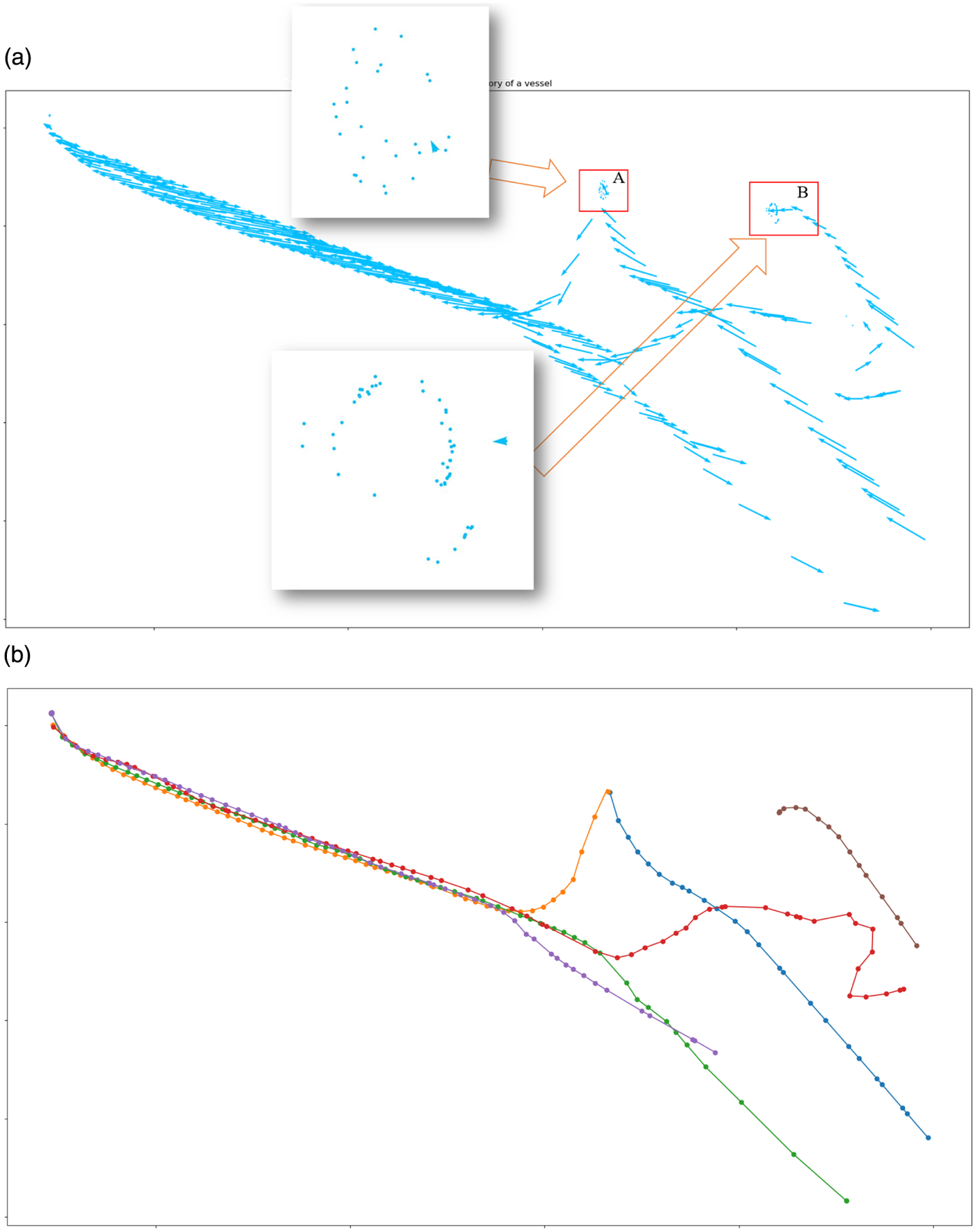
(1) Read data from the database, analyse the raw data and then classify the data according to the voyage numbers. With the ship's MMSI (maritime mobile service identity) number as the index, all the voyages of the ship at certain period of time can be obtained, as shown in Figure 4(a). It can be seen that the trajectory data of the ship contains various voyage numbers, including navigating trajectories and anchoring trajectories. All the voyages are separated and the data of anchoring trajectories are removed. The trajectory classified according to voyage numbers is as shown in Figure 4(b).
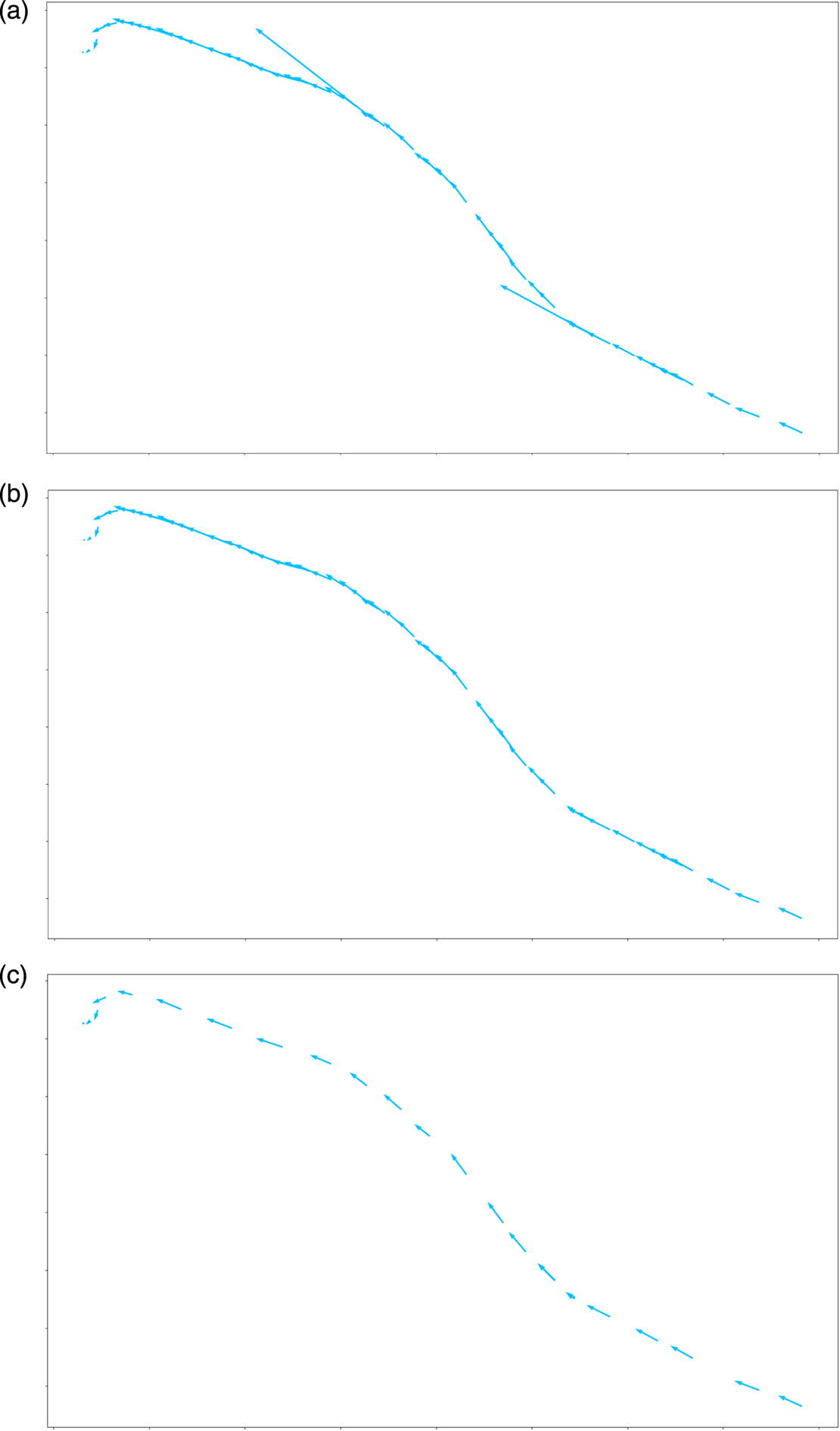
(2) Under normal circumstances, the speed of the ship sailing in the port should not exceed 15 knots. By eliminating the abnormal data in each voyage, the normal trajectory can be obtained, as shown in Figure 5(b). Since the original data is not time-series data with equal intervals, the cubic spline is used to interpolate the trajectory smoothly, and the sampling step is 5 min. Through processing the original AIS data from Tianjin port, China, in 2014, a total of 50,292 ship historical trajectories were obtained.
(3) Considering that ships have opposite headings when entering and leaving the port, to study the law of ship movement further, the trajectories of inbound and outbound ships are distinguished.
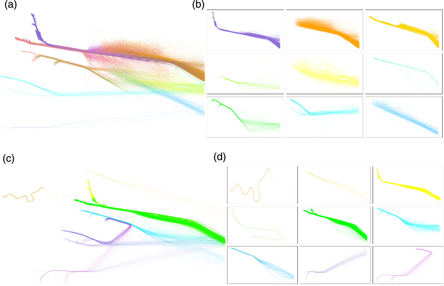
(4) The inbound and outbound trajectories of the ship are analysed separately and classified according to the starting point and the ending point. The classification result is shown in Figure 6. The DBSCAN (density-based spatial clustering of applications with noise) algorithm is used to cluster the starting points and the ending points of the trajectory, respectively. The point clusters obtained are combined into pairs to obtain the final classification of the trajectories. By clustering the trajectories, the ship's inbound trajectories are divided into 16 categories and its outbound trajectories are divided into 11 categories. Figure 6 shows some results of trajectory clustering.
Process of dividing voyages from the original trajectory data: (a) the blue arrow indicates the transient vector of the ship; the length of the trajectory vector in areas A and B is short, indicating that the speed of ships in the area is low and it is anchoring data. (b) original data divided into six voyages. The trajectories of the different voyages are represented by different colours.

(a) Ship trajectories containing abnormal values; (b) ship trajectories after abnormal values are removed; (c) trajectory vector set after the trajectories are interpolated using a cubic spline function.

Clustering results of inbound and outbound trajectories: (a) classification of inbound trajectories, (b) subclasses of inbound trajectories (c) classification of outbound trajectories, (d) subclasses of outbound trajectories. Different categories are represented by different colours.

3.2. Mapped meshing of the sea area
To research the behavioural features of ships in the port, it is necessary to discretise the instantaneous state of the ship into corresponding grids. With the grid as the basis unit, the statistical characteristics of the historical trajectories in the geospatial space of the ship in the port can be obtained. The distribution of ships' states in each grid is calculated and the thresholds of these characteristics are recorded. When a ship to be detected enters these grid areas, the abnormal state detection can be carried out according to the threshold values. Meshing mainly consists of two processes:
(1) Determine the grid width. The average speed of the ship sailing in the port is obtained through statistics, and the movement distance of the ship at the average speed for 1 min is defined as the grid width. It is calculated that the average speed in the port is 4·7 kn, so, the grid width is 150 m.
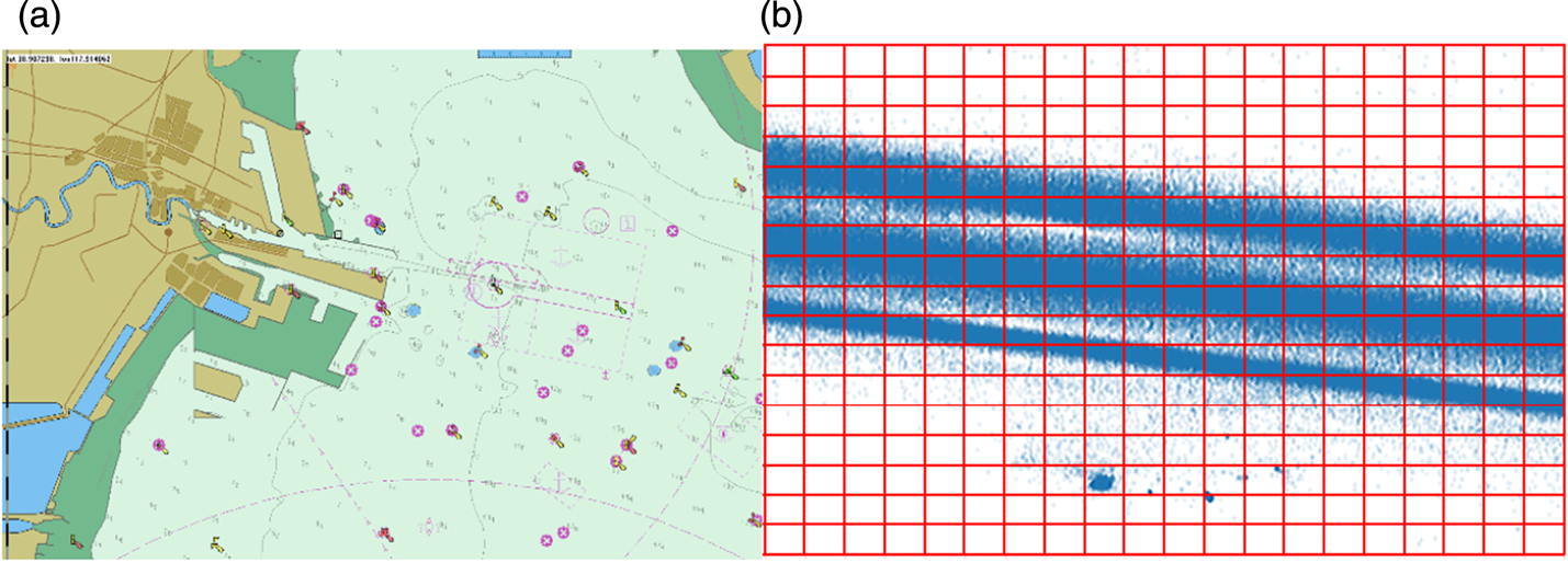
(2) Mesh the entire sea area to be studied. Determine the boundary of the sea area to be studied: the minimum boundaries of all ship trajectories are considered as the vertices of the mesh. Specific parameters are as follows: upper left corner (117·49946E, 39·20094N), upper right corner (118·20099E, 39·20094N), lower left corner (117·49946E, 3859899N), lower right corner (118·20099E, 38·59899N). According to the grid width determined in (1), in this study, the sea area to be studied is divided into 231,920 grids. The range of the sea area to be studied is shown in Figure 7(a). Figure 7(b) shows the partial mesh area extracted from the sea area to be studied.
(a) Sea area studied; (b) partial grid area after the sea area is divided. The points marked blue in the figure represent historical data of ship trajectories.

3.3. Ship abnormal behaviour detection model
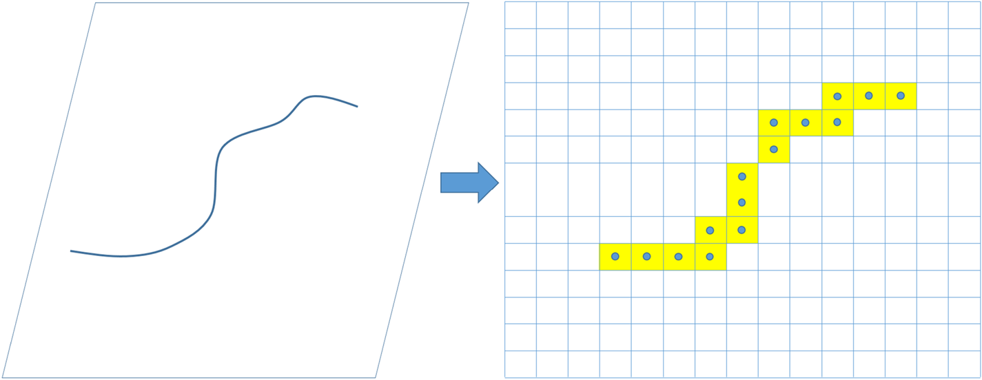
Definition 2: Trajectory represented based on grid: T grid is a trajectory represented based on grid and T grid = {gridi}, i ∈ [1, n], where gridi is the grid index corresponding to position p i of trajectory T in definition 1, meanwhile n is the length of trajectory T. Which is shown in Figure 8.
Ship trajectory converted to grid-based representation.

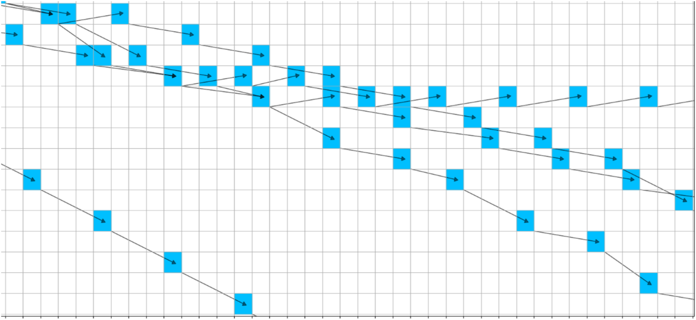
The process of data preprocessing mentioned above classifies the historical trajectories of ships. In this section, a probabilistic directed graph model for each category of trajectories will be constructed. After the position points in each trajectory are discretised into the corresponding grids, grid-based trajectories can be obtained. Two meshes connected to each other form a directed edge, and these two meshes are two nodes of the directed edge. Extract N i trajectories from each category to build a directed graph (as shown in Figure 9).
 $$N_i =\vert C_i \vert \quad i\in n$$
where C i is trajectory category, | · | is calculation of the trajectory numbers of each category and n is the number of the trajectory categories.
Definition 3: Directed graph of trajectories: The directed graph established with the trajectories represented by the grids is expressed as G(V, E, W), where V is a set with grids as the nodes, e ∈ E is the directed edge formed between two grid nodes, and w ∈ W is the weight of each directed edge, that is, the probability of converting from node v i to node v j.
Trajectory directed graph constructed based on a grid representation. Blue boxes are the grid index corresponding to the ship's geographical point, representing the node of the directed graph; black arrows indicate the directed edge between adjacent nodes.

3.3.1. Abnormal detection model of speed and course
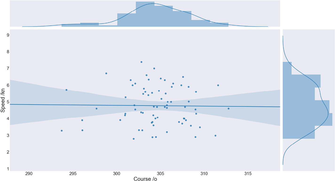
The statistical characteristics are obtained by analysing the course and speed distribution of the ships in each node in the directed graph (Figure 10), and by calculating the mean and variance of the ships' courses and speed dimensions in each node. The abnormal state detection model is then constructed according to the statistical characteristics of the obtained data. From the perspective of statistics, when the overall complies with the general normal distribution, the probability of the sample falling within the area with three-times standard deviation is 99·7%. Considering the error impact of the data itself, 99·7% of the raw data in each node are selected to build a normal state model. The calculation method is as follows:
Historical heading and speed distribution of ships in a node. The horizontal axis is the course distribution, and the vertical axis is the speed distribution.

 $$\begin{align} \bar {x}&=\frac{1}{n}\sum\limits_{i=1}^n {x_i }\end{align}$$
 $$\begin{align} \sigma ^2&=\frac{1}{n-1}\sum\limits_{i=1}^n {(x_i -\bar {x})^2} \end{align}$$
In Equation (1), n is the capacity of the sample, representing the total number of the location points of the ship in the node,  $\bar {x}$ is the mean value of the sample x ∈ {Course, Speed}. In Equation (2), σ 2 is the sample variance.
As shown in Figure 10, the ships' states in each node approximately comply with normal distribution  $N_{i} \sim ( \mu _{i}, \; \sigma _{i} ^{2}), \; i \in \{ \mbox{Course}, \; \mbox{Speed} \} $ both in course and speed dimensions. Given the confidence
 $( 1-\alpha ) \ast 100\% $, where α = 0 · 003 is of significant level, the confidence interval can be calculated by the following equations:
 $$\begin{align} &\mbox{Interval}(b_{\rm low}^i, b_{\rm up}^i )=(1-\alpha )\ast 100\% \end{align}$$
 $$\begin{align} & b_{\rm low}^i, b_{\rm up}^i =\mu \pm 3\ast \sigma \quad i\in \{\mbox{Course},\mbox{Speed}\} \end{align}$$
In Equation (5),  $b_{\rm up}^{i}, \; b_{\rm low}^{i}$ are the upper and lower boundaries of the normal value domain in the state anomaly detection model.
For state anomaly detection, the determination of thresholds are statically dependent on the distribution characters of course and speed in the current node from historical ships data. The normal state threshold  $( b_{\rm up}^{\rm Course}, \; b_{\rm low}^{\rm Course}, \; b_{\rm up}^{\rm Speed}, \; b_{\rm low}^{\rm Speed}) $ of ships is defined. Therefore, when the current heading C t or speed S t of a ship is outside the normal threshold, it is defined as a state anomaly.
 $$\begin{align} &\begin{cases} \mbox{Abnormal Course}, & \hbox{if } C_t < b_{\rm low}^{\rm Course} \mbox{ or }C_t >b_{\rm up}^{\rm Course}\\ \mbox{Normal}, & \hbox{if }b_{\rm low}^{\rm Course} \le C_t \le b_{\rm up}^{{\rm Course} } \end{cases} \end{align}$$
 $$\begin{align} &\begin{cases} \mbox{Abnormal Speed}, & \hbox{if }S_t < b_{\rm low}^{\rm Speed} \mbox{ or }S_t >b_{\rm up}^{\rm Speed} \\ \mbox{Normal}, & \hbox{if }b_{\rm low}^{\rm Speed} \le S_t \le b_{\rm up}^{\rm Speed} \end{cases} \end{align}$$
C t in Equation (6) and S t in Equation (7) are the instantaneous course and speed of a ship, respectively, at the current moment.
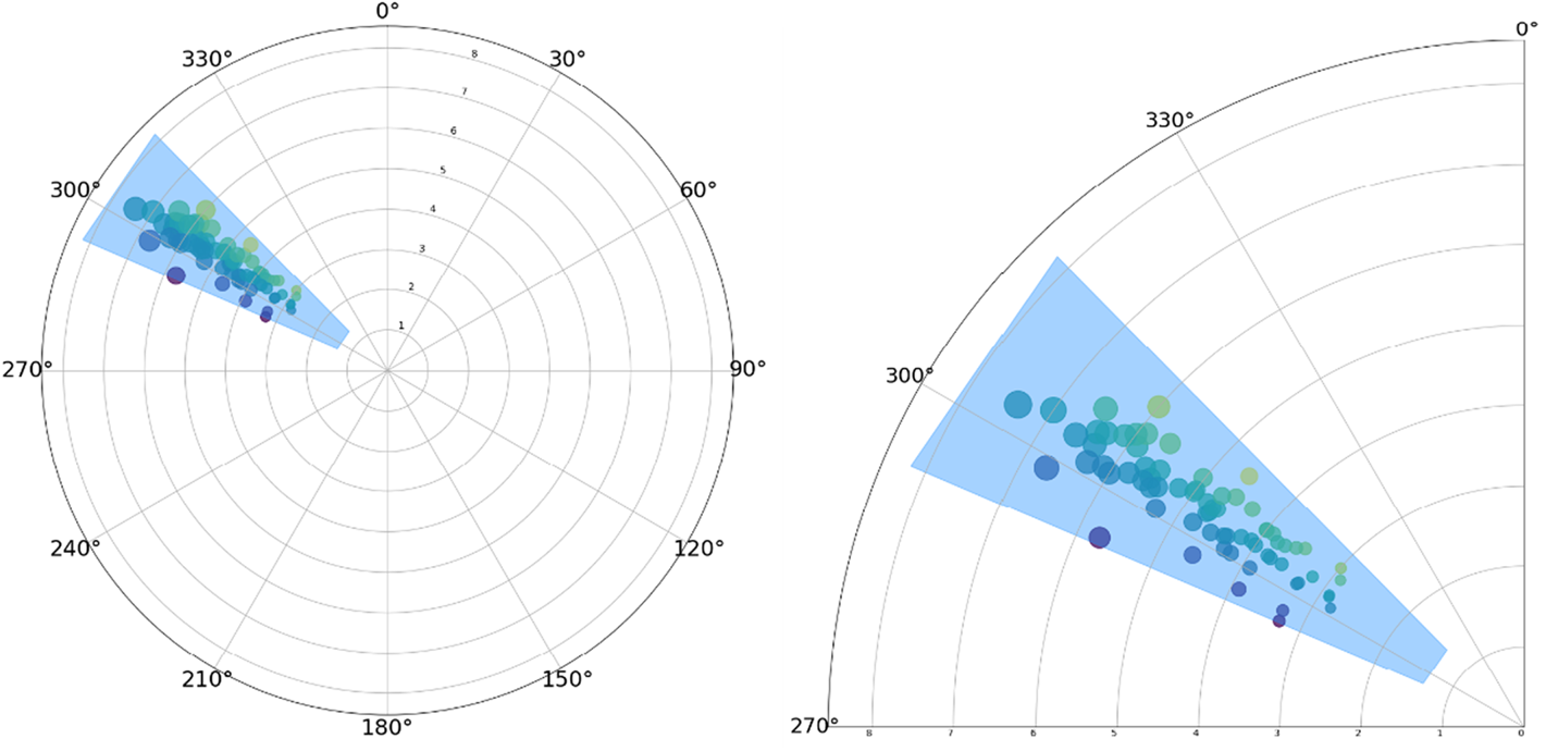
In this paper, the course-speed distribution is represented by polar coordinates, and the state data in each node is represented under polar coordinates. In Figure 11, the coloured data points are the course and speed state of the ships, and the blue polygonal box indicates that the probability of speed and course of a ship being within the area is 99·7%.
The normal state threshold area of ships with three standard errors in a node.

3.3.2. Ship position anomaly detection based on probabilistic directed graph model
Construct candidate set of the child nodes: According to the directed graph established in Section 3.3, the current node is taken as the parent node. Under the condition of the given parent node, the conditional probability of each child node is calculated to obtain a probability directed graph.
 $$P(v_i )=P(v_i \vert \mbox{Par})P(\mbox{Par})\quad i=1,2,\ldots,n$$
 $$\sum\limits_{i=1}^n {P(v_i \vert \mbox{Par})} =1$$
where Par is the parent node, that is, the current node, v i is the ith child node, and n is the number of child nodes of the current node. P(Par) represents the prior probability of the parent node.
In the probabilistic directed graph model, given the current node, search all the child nodes of the node, construct candidate set of the child nodes {child}, calculate the conditional probability of each child node, arrange them in descending order, and screen the possible child nodes in the confidence interval according to the confidence level set by the user. If the position of the ship at the next moment is not in these sub-nodes, then the behaviour of the ship can be defined as a position anomaly.
Trajectory prediction: Given the current node, search dynamically for possible trajectory sets of the ship at a future time, calculate the probability of each trajectory, and take the trajectory with the highest probability as the predicted trajectory of the ship at the future time. Construct set {T grid} of predicted trajectories. Each trajectory  $T_{\rm grid}^{i} $ is a chain
 $v_{1}^{j} \to \cdots \to v_{n}^{j}, \; \ j\in N \{ T_{\rm grid} \} $ with n nodes. For i = 1, …, n − 1; j ∈ N{T grid} calculate
 $P( v_{i+1}^{j} ) $ based on
 $P( v_{i}^{j} ) $. The probability of each predicted path can be calculated by the following formula:
 $$P(T_{\rm grid}^j )=\prod\limits_{i=1}^{n-1} {P(v_{i+1}^j \vert v_i^j )P(v_i^j )\quad j\in N\{T_{\rm grid} \}}$$
where N{T grid} represents the trajectory number in the predicted trajectory set. The trajectory with the highest calculated probability is taken as the predicted trajectory of the ship at a future time:
 $$ \mbox{predict}\_\mbox{path}=\mathop {\arg \,\max }\limits_j P(T_{\rm grid}^j )$$
where  $\mbox{predict}\_\mbox{path}$ is the maximum probability predicted trajectory given by the model.
Simple extrapolation model: The model is used to extrapolate the ship's state by one step of 5 min according to the current state information of the ship. First, define the state vector of the ship:
 $$S_k =[s_x^k, \dot {s}_x^k, s_y^k, \dot {s}_y^k ]^{{\rm T}}$$
where S k is the state of the ship at time k, and  $( s_{x}^{k}, \; s_{y}^{k} ) $ represent the longitude and latitude coordinates of the ship's location at time k, and
 $( \dot {s}_{x}^{k}, \; \dot {s}_{y}^{k} ) $ are the horizontal and vertical velocities of the ship.
 $$S_{k+1} =FS_k$$
 $$F=\left[ {{\begin{matrix} 1 & T & 0 & 0 \\ 0 & 1 & 0 & 0 \\ 0 & 0 & 1 & T \\ 0 & 0 & 0 & 1 \\ \end{matrix} }} \right]$$
where F is the state transition matrix and T is the extrapolation time step where T = 5 min.
 $$\mbox{pos}_{k+1} =\left[\begin{matrix} 1 & 0 & 0 & 0\\ 0 & 0 & 1 & 0 \end{matrix}\right]S_{k+1}$$
where posk+1 is the position of the ship extrapolated by the model and S k+1 is the state of the ship at time k + 1.
The ship's position posk+1 obtained by the extrapolation model is compared with the candidate set of child nodes {child} and the predicted trajectory  $\mbox{predict}\_\mbox{path}$ obtained above. If the ship's position after 5 min is located in the candidate set of child nodes or predicted trajectory, it can be judged that the ship's position is normal; otherwise, the ship has a tendency of abnormal position.
4. EXPERIMENTAL DESIGN AND RESULT ANALYSIS
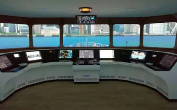
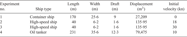
A maritime simulator was used to test the performance of the proposed abnormal behaviour detection model. Maritime simulators simulate different situations in ship manoeuvring and they are now widely used in maritime education and training, as well as in engineering demonstrations and scientific research in related fields (as shown in Figure 12). In this paper, the maritime simulator was used as an experimental platform. First, the hydrological conditions of Tianjin port were modelled. Four experiments of ship inbound operations were simulated to detect the abnormal behaviour of the ship in real time. Information on the ships in the simulated experiments is shown in Table 1.
Maritime simulator experimental platform.

Information about ships in the simulated experiments.

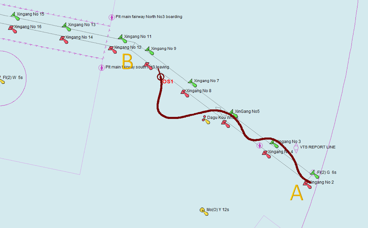
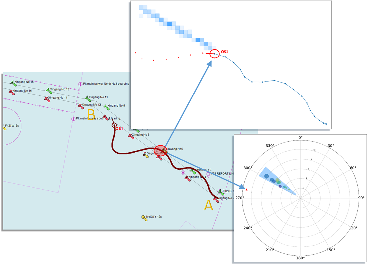
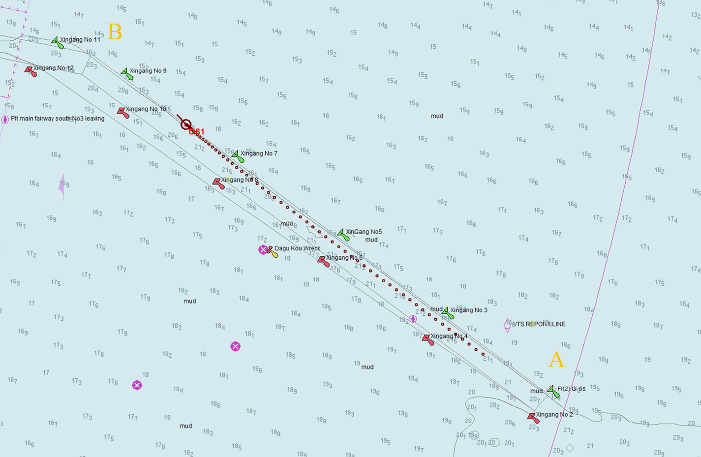
Experiment 1: Simulate the process of a ship moving from the entrance of the two-way channel (point A) to a turning point (B). As shown in Figure 13, the ship sailed freely in the channel, and sometimes deviated from the channel, while maintaining high-speed navigation throughout the entire voyage. The overall sailing time was 28 min. Real-time detection of the abnormal behaviours of the ship's navigation was carried out, and the test results are shown in Figure 14.
Ship operation simulation experiment, trajectory 1. Starting point A is the entrance to the channel, and point B is the turning point. The red sign OS1 represents the current location of the ship.

Presentation of results of detection of abnormal behaviour of the ship at t = 17 min.

Figure 14 shows the results of detection of an anomaly by the ship at the 17th minute. The red triangle mark in the polar chart indicates the current course and speed of the ship. It is judged according to the current course and speed value of the ship that the model is not in the normal area, so it can be determined that the ship is in an over-speed and yaw state, which could be defined as a state anomaly. The red mark OS1 in the trajectory prediction graph indicates the current position of the ship, and the blue highlight area is the normal navigation mode predicted by the model. The ship in this mode should sail in a northwesterly direction, but it is detected by the model that the ship is deviating from the normal navigation mode, so it registers as an abnormal behaviour.
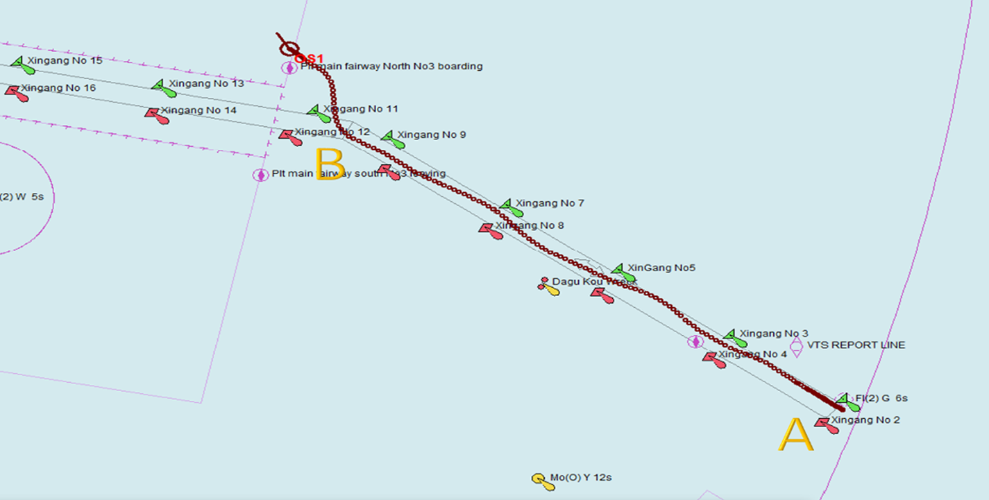
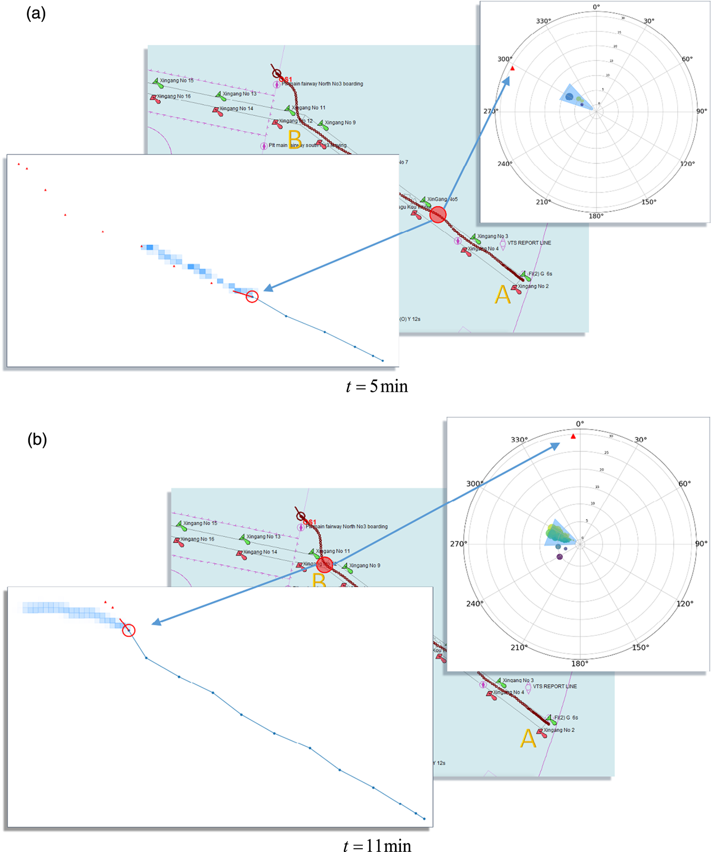
Experiment 2: Simulate the process of a ship moving from the entrance (point A) of the two-way channel to the turning point (B) (Figure 15). The ship is in a state of high-speed navigation throughout the simulation process. After reaching the turning point, the ship heads north into the anchorage, deviating completely from the navigation channel specified by the traffic separation scheme. The entire simulated sailing lasts 14 min. Figure 16 shows the state analysis of the ship at t = 5 min and t = 11 min.
Ship operation simulation experiment, trajectory 2. Starting point A is the entrance to the channel, and point B is the turning point. The red sign OS1 represents the current location of the ship.

Presentation of results of detection of abnormal behaviours of the ship. (a) t = 5 min (b) t = 11 min.

As shown in the polar plot in Figure 16, the speed of the ship is nearly 30 kn, which is much faster than the 10 kn limit in this area, so it is identified by the model as a severe over-speed. In Figure 16(a), although the ship is over-speeding at t = 5 min, it is still sailing in the channel and its course is normal. The actual position of the ship at the future moment indicated by the red triangle sign is also in the highlighted area of the model prediction. As shown in Figure 16(b), at t = 11 min the ship's heading is close to true north deviating from the allowable value of the normal navigation mode, and its course is now abnormal. The blue highlight area indicates the normal sailing mode of ships in the channel. It can be seen from the position of the ship at a future time, indicated by the red triangle sign, that it is about to deviate from the channel.
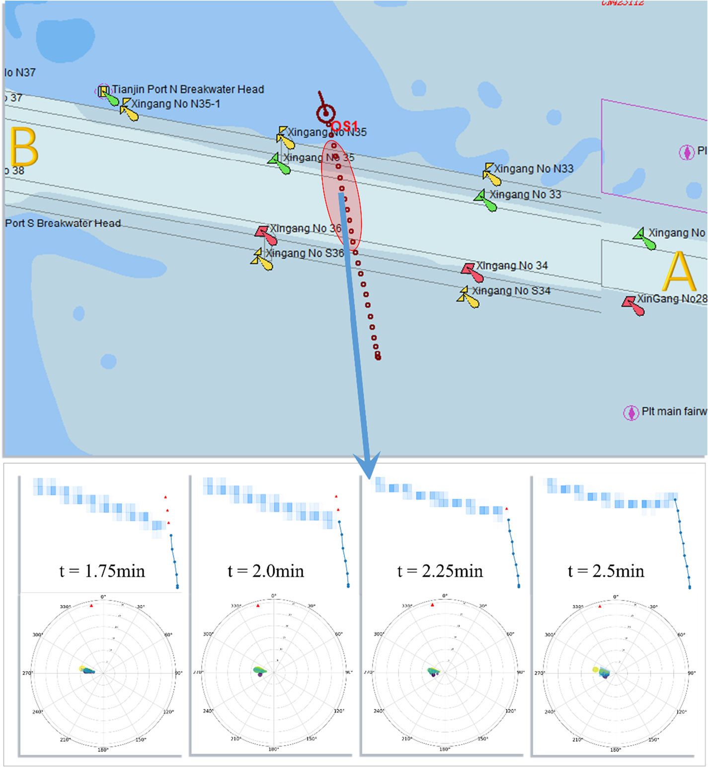
Experiment 3: Simulate a ship sailing from south to north across the channel at a speed of 30 kn. The entire simulation process lasts 2·5 min. The test results are shown in Figure 17 which shows the results of abnormality detection after the ship enters the channel, that is, t = 1 · 75 min, t = 2 · 0 min, t = 2 · 25 min, t = 2 · 5 min, where t is the current time. The model can detect that the ship is sailing north at a speed of 30 kn, which is much faster than the maximum speed allowed in the channel, so the ship is in a state anomaly. The blue highlight area given by the model indicates that the ship should sail according to the normal navigation mode within the channel; however, continuous detection results indicate that the ship has deviated from the normal navigation mode.
Presentation of results of detection of abnormal behaviour of the ship, crossing the channel.

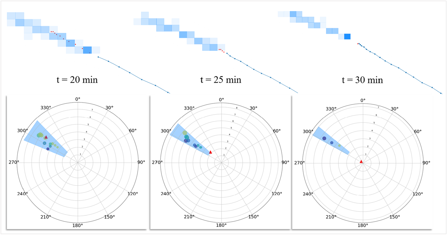
Experiment 4: In the navigation simulator, the simulated ship sails in section A–B of the channel and remains in the channel all the way. At the 20th minute of the voyage, the ship slows down suddenly until its speed is reduced to 0 kn. The whole simulated voyage time lasts 31 min, as shown in Figure 18. Figure 19 shows the detection results of the model at 20 min, 25 min and 30 min, respectively. It can be seen that the model detected that although the ship was sailing in the channel, its speed decreased by 5 kn within 10 min, so it was judged that the ship had an abnormal change of speed. Finally, the ship stopping in the channel was detected.
Ship operation simulation experiment, trajectory 4.

Presentation of results of detection of abnormal behaviour of the ship, change of speed.

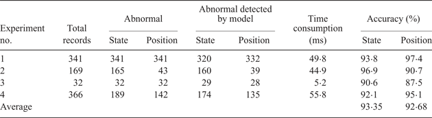
Table 2 shows the collated results of the simulated experiments. It can be seen that lines 2–5 of the content respectively represent four experimental processes. The model designed in this paper can detect the abnormal behaviour of ships of different categories and scales, and the model satisfies the requirements in terms of universality. The seventh column in Table 2 shows the time consumption of the four simulation tests respectively. With the increase of sample size, the time consumption of the model in the detection process does not increase significantly, showing a good performance in terms of real-time performance. The accuracy of the model recorded in columns 8 and 9 in Table 2 was 93·35% on average for the detection of ship state anomalies, and 92·68% on average for the detection of ship position anomalies.
Data results of the simulated experiments.

5. CONCLUSION AND PROSPECTS
In this paper, the navigation modes of ships entering and leaving a port are classified by preprocessing the original AIS data and using a density-based clustering method, including 16 categories of navigation modes of inbound vessels, and 11 categories for outbound vessels. The trajectory data are discretised with a mesh-based method, the navigation mode of each category is learned, and the probabilistic directed graph model is established. The statistical characteristics of each node of the ship in the probabilistic directed graph are used to detect any abnormal states of ships in real time. For the current position of the ship, the probabilistic graph model is used to calculate the trajectory of the ship with the highest probability in the normal navigation mode, which is used as the predicted trajectory of the ship to detect whether the navigation behaviour of the ship is abnormal. To verify the validity of the proposed model, four experiments were designed to simulate the ship navigation based on a maritime simulator platform. It is shown by the experimental results that the proposed model can conduct real-time detection of the course and speed of the ship effectively and judge whether it had surpassed relevant thresholds of course or speed. Moreover, it can also judge whether there was potential abnormal behaviour by predicting the normal sailing trajectory of the ship. Abnormal behaviours of ships were detected successfully by the model in the three designed simulation experiments. The ship behaviour anomaly detection system can automatically identify a ship's abnormal behaviour, issue an alarm, give advice for safe navigation and improve the navigation safety of the port's waters, and thus free the maritime supervisors from a demanding task.
The disadvantage of this model is that it can only detect certain limited abnormal behaviours of ships; it cannot detect abnormal behaviours such as sudden shifting and wandering of a ship in the channel. In the future, this study will focus on the detection of abnormal behaviours of ships such as loitering, random navigation and illegal occupation of waterways. Thereafter, an automated decision support system will be designed to assist with intelligent navigation. Another limitation is that, since we only have the data set of Tianjin port in China, this paper does not involve using multiple data sets to test the model. In the future, AIS data from different ports will be studied using the model in this paper in order to make it more versatile.
ACKNOWLEDGEMENTS
This research is supported by the project of Intelligent Ship Testing and Verification, 2018/473, China and the Fundamental Research Funds for the Central Universities [No. 3132019312]. The authors are also grateful for support from the Maneuvering Simulation of Yunnan Inland Shipping Ships [No. 851333] and the Liaoning Natural Science Foundation—Research on Key Technologies of Navigation Vision Enhancement System [20170540091].}