2.1. Experimental set-up

The experiments were performed on a semi-open, five-bladed mixed-flow pump with a six-vaned diffuser, as illustrated in figure 1(a ). It is designed for flow rate ( $\textit {Q}_{d}$ ) 0.0346 m $^{3}$ s⁻¹ and head ( $\textit {H}_{d}$ ) 2.57 m at rotational speed ( $\textit {n}_{d}$ ) 1450 rpm. This corresponds to a BPF $f_{\textit{BPF}} \approx 121$ Hz. Based on the impeller outlet diameter ( $D_2=0.18$ m) and tip speed, the Reynolds number is $Re \approx 2.2 \times 10^6$ , indicating a fully turbulent flow regime. For all experiments, the tip clearance was maintained at a constant 0.8 mm, corresponding to a non-dimensional clearance of 0.44 % of the impeller outlet diameter. This value not only is representative for the pump, but also allows the present analysis to build directly upon a well-characterised baseline case from the previous studies (Han & Tan Reference Han and Tan2023a , Reference Han and Tanb ; Han, Tan & Han Reference Han, Tan and Han2024).

The pump was tested in a closed-loop hydraulic facility at Tsinghua University, as shown in figure 1(b), that has yielded previously published results (Lu et al. Reference Lu, Tan, Han and Liu2022; Han & Tan Reference Han and Tan2023a ). The uncertainties of the primary measured variables are as follows: flow rate (Q) is $\pm 0.2\,\%$ , torque (T) is $\pm 0.2\,\%$ , rotational speed (n) is $\pm 1$ rpm (equivalent to $\pm 0.069\,\%$ at the design point), and inlet/outlet pressures (p) are $\pm 0.065\,\%$ . Based on these instrument accuracies, the maximum relative uncertainties for the head H, shaft power P, and pump efficiency $\eta$ are estimated to be $\pm 0.15\,\%$ , $\pm 0.21\,\%$ and $\pm 0.32\,\%$ , respectively.

Figure 1.

Experimental set-up: (a) the test mixed-flow pump; (b) the closed-loop hydraulic test rig.

The primary focus of this study, the unsteady pressure on the stationary shroud, was investigated using an array of eight flush-mounted, high-frequency pressure sensors (Model CYG515A, range 0–200 kPa (absolute), accuracy 0.25 %), as detailed in figure 2. Flush-mounting is critical to prevent artefacts from flow-induced sensor vibration or cavity resonance (Camussi et al. Reference Camussi, Grilliat, Caputi-Gennaro and Jacob2010). The sensors were installed in 5 mm diameter ports, each featuring a pressure tap with 0.7 mm diameter orifice and 1 mm depth. This small orifice size is crucial for minimising spatial-averaging effects, which can attenuate the signature of high-wavenumber turbulent structures (Hu Reference Hu2022; Huang et al. Reference Huang, Duan, Casper, Wagnild and Bitter2024).

Figure 2.

Arrangement of the eight high-frequency dynamic pressure sensors on the shroud wall, showing (a) the schematic model and (b) a photograph of the experimental set-up. The sensors are positioned at dimensionless axial locations $z^*=(z-z_l)/(z_t-z_l) = -2.38, -0.46, 0, 0.33, 0.67, 1, 1.54, 2.15$ , corresponding to sensors 1–8, respectively. Sensor 3 aligns with the blade tip leading edge, and sensor 6 with the trailing edge. For installation purposes, sensors 3 and 5 are circumferentially offset by $10^{\circ }$ .

The sensors were arranged sequentially along the shroud to capture the axial development of the flow. Their positions are defined by the dimensionless axial coordinate $z^*=(z-z_l)/(z_t-z_l)$ , where $z$ is the axial position, and $z_l=0.106$ m and $z_t=0.128$ m are the axial positions of the blade tip leading edge and trailing edge, respectively. The dimensionless locations for sensors 1–8 are $-2.38, -0.46, 0, 0.33, 0.67, 1, 1.54, 2.15$ . Notably, sensor 3 aligns with the leading edge, and sensor 6 with the trailing edge. This axial array is complemented by circumferential offset $10^{\circ }$ for sensors 3 and 5 relative to the main sensor line. This strategic offset is dual-purpose: it enables the capture of azimuthal phase variations, essential for reconstructing spatio-temporal flow features (Kameier & Neise Reference Kameier and Neise1997), while also ensuring adequate physical spacing between ports to mitigate potential acoustic crosstalk or sensor-induced flow alterations.

Data were acquired synchronously using a 16-channel acquisition system at sampling frequency 5120 Hz, which is more than 40 times the BPF, and ensures resolution of at least the first 20 harmonics. This bandwidth is adequate for capturing the primary energy-containing frequencies associated with rotor–stator interaction, as demonstrated in similar pump configurations (Luo et al. Reference Luo, Ge, Feng, Zhu, Li and He2024). At each measured operating conditions, signals were recorded for 15 s, equivalent to approximately 362.5 rotor revolutions, ensuring robust statistical convergence of phase-averaged quantities (Feng, Benra & Dohmen Reference Feng, Benra and Dohmen2007). A notch filter was applied to the raw data to remove noise at the 50 Hz power line frequency and its harmonics. The total uncertainty for the unsteady pressure signal, accounting for the data acquisition system, is determined to be within $\pm 0.82\,\%$ .

2.2. Numerical set-up

The flow within the mixed-flow pump is simulated by solving the spatially filtered, incompressible Navier–Stokes equations. The governing equations for the resolved velocity field $\hat {u}_i(\boldsymbol{x},t)$ and pressure field $\hat {p}(\boldsymbol{x},t)$ are given by

(2.1) \begin{align} \frac {\partial \hat {u}_i}{\partial x_i} &= 0, \\[-12pt]\nonumber \end{align}

(2.2) \begin{align} \frac {\partial \hat {u}_i}{\partial t} + \frac {\partial (\hat {u}_i \hat {u}_{\!j})}{\partial x_{\!j}} &= -\frac {1}{\rho }\frac {\partial \hat {p}}{\partial x_i} + \nu\, {\nabla} ^2 \hat {u}_i - \frac {\partial \tau _{\textit{ij}}}{\partial x_{\!j}}, \end{align}

where $\hat {({\cdot })}$ denotes spatial filtering. The unclosed term $\tau _{\textit{ij}} = \widehat {u_i u_{\!j}} - \hat {u}_i \hat {u}_{\!j}$ is the subgrid-scale stress tensor, representing the effect of unresolved turbulent scales.

The accurate resolution of multi-scale turbulent structures is paramount for this study. These structures encompass not only the fine-scale dynamics associated with the formation, development and subsequent breakdown of the TLV, but also the large-scale coherent motions originating from the unsteady rotor–stator interaction. To address these phenomena with a high degree of fidelity yet within a computationally feasible framework, the stress-blended eddy simulation (SBES) model (Menter & Egorov Reference Menter and Egorov2010), as implemented in ANSYS CFX, was adopted for all simulations.

The foundation of the SBES model is the shear-stress transport (SST) $k{-}\omega$ model (Menter Reference Menter1994). The SST model is widely recognised for its robust performance in flows with attached boundary layers and moderate separation. It blends the $k{-}\omega$ model in the near-wall region with the $k{-}\varepsilon$ model in the freestream and wake regions. The transport equations for the turbulent kinetic energy $k$ and the specific dissipation rate $\omega$ are

(2.3) \begin{equation} \frac {\partial (\rho k)}{\partial t} + \frac {\partial (\rho u_{\!j} k)}{\partial x_{\!j}} = P_k - \beta ^* \rho \omega k + \frac {\partial }{\partial x_{\!j}} \left [ (\mu + \sigma _k \mu _t) \frac {\partial k}{\partial x_{\!j}} \right ]\!, \end{equation}

(2.4) \begin{equation} \frac {\partial (\rho \omega )}{\partial t} + \frac {\partial (\rho u_{\!j} \omega )}{\partial x_{\!j}} = \frac {\alpha }{\nu _t} P_k - \beta \rho \omega ^2 + \frac {\partial }{\partial x_{\!j}} \left [ (\mu + \sigma _\omega \mu _t) \frac {\partial \omega }{\partial x_{\!j}} \right ] + 2(1-F_1)\frac {\rho \sigma _{\omega 2}}{\omega } \frac {\partial k}{\partial x_{\!j}} \frac {\partial \omega }{\partial x_{\!j}}, \end{equation}

where $P_k$ is the production term of turbulent kinetic energy, and $\mu _t$ is the turbulent eddy viscosity. All model coefficients and the blending function $F_1$ are as defined by Menter (Reference Menter1994).

The core concept of SBES is the direct blending of the Reynolds stress tensors. The total turbulent stress tensor $\tau _{\textit{ij}}^{\textit{SBES}}$ is a weighted combination of the SST and large eddy simulations (LES) components via a shielding function $f_s$ :

(2.5) \begin{equation} \tau _{\textit{ij}}^{\textit{SBES}} = f_s \tau _{\textit{ij}}^{\textit{SST}} + (1-f_s) \tau _{\textit{ij}}^{\textit{LES}}. \end{equation}

Here, $\tau _{\textit{ij}}^{\textit{SST}}$ is computed by the SST $k{-}\omega$ model, and $\tau _{\textit{ij}}^{\textit{LES}}$ is the subgrid-scale (SGS) stress from LES. The shielding function $f_s$ is designed to protect the boundary layer, ensuring that it remains fully in SST mode, with $f_s=1$ near the wall, and smoothly transitioning to $f_s=0$ in the core flow.

To facilitate the transition from SST to LES, SBES introduces an additional sink term $\varepsilon _{\textit{SBES}}$ into the SST $k$ -equation to mimic the energy dissipation at subgrid scales:

(2.6) \begin{equation} \varepsilon _{\textit{SBES}} = \beta ^* \rho \omega k \times f_{\textit{SBES}}, \end{equation}

where the blending function $f_{\textit{SBES}}$ is defined as

(2.7) \begin{equation} f_{\textit{SBES}} = \max \left [ \frac {L_t}{C_{\textit{SBES}}\varDelta _{\textit{SBES}}}(1-f_s), 1 \right ] - 1. \end{equation}

Here, $L_t = \sqrt {k}/(\beta ^*\omega )$ is the turbulent length scale, $C_{\textit{SBES}}$ is a model constant, and $\varDelta _{\textit{SBES}}$ is the local grid scale. This formulation ensures that the dissipative term is activated in regions where the grid resolution is fine enough to resolve turbulent eddies, thus enabling a seamless transition to LES mode.

The computational domain (figure 3 a) includes the impeller, diffuser and extended inlet/outlet pipes. The outlet is simplified as a straight pipe. The locations of pressure monitoring points are set to be identical to the experimental positions. To ensure high-fidelity resolution of the multi-scale turbulent structures, a structured O-grid topology is employed in the near-wall and tip clearance regions. The numerical integrity of the simulation was established through a grid independence study using four sets of meshes. As shown in table 1, the predicted head and efficiency exhibited clear asymptotic behaviour as the mesh was refined. The discrepancy between meshes 3 and 4 is less than 0.5 % for head and 0.2 % for efficiency. Consequently, mesh 3, consisting of approximately $6.02 \times 10^6$ elements, was selected to balance computational cost with the required spatial resolution.

Table 1.

Grid independence study results for the mixed-flow pump at the design point.

For this selected mesh, the height of the first grid layer was strictly controlled to maintain non-dimensional wall distance $y^+ \lt 1$ (figure 3 b). This ensures that the SST component of the SBES model accurately resolves the viscous sublayer, providing a reliable wall boundary condition for the LES regions (Li et al. Reference Li, Huang, Sun, Pan, Li and Bai2023). Crucially, the fidelity of this numerical set-up in capturing key flow features is demonstrated in figure 3(c). The simulation effectively resolves the complex three-dimensional topology. The spatial distribution of the SBES shielding function ( $f_s$ ) is examined in figure 3( d). The results confirm that the entire tip clearance region and the trajectory of the TLV are located within the LES-active zone ( $f_s = 0$ ), where multi-scale turbulent structures are directly resolved rather than modelled. The Reynolds-averaged Navier–Stokes (RANS) mode ( $f_s = 1$ ) is appropriately restricted to the thin near-wall boundary layers.

Figure 3.

Schematic of the computational domain and numerical fidelity verification. (a) Overall view of the computational domain with mesh details. (b) Distribution of $y^+$ on blade and hub surfaces. (c) Vortex structures visualised by $Q$ -criterion ( $Q_{{iso}}=10^6$ ), coloured by time-averaged relative velocity. (d) Distribution of the SBES shielding function $f_s$ on multiple planes, where $f_s=0$ (blue) denotes the LES region, and $f_s=1$ (red) denotes the RANS region.

A hybrid scheme combining a second-order central difference scheme with a first-order upwind scheme is employed for the advection term. A second-order backward Euler scheme is used for the transient term. The time step is set to $\Delta t = 2.29885 \times 10^{-4}$ s, which corresponds to a $2^\circ$ rotation of the impeller per step. This temporal resolution yields sampling frequency approximately 4350 Hz, which is more than 35 times the BPF ( $f_{\textit{BPF}} \approx 121$ Hz). To ensure temporal independence of the numerical results, a sensitivity study was conducted using three different time steps corresponding to $1^\circ$ , $2^\circ$ and $4^\circ$ of impeller rotation per step. The amplitudes and phases of $f_{\textit{BPF}}$ and its primary harmonics were compared at the shroud monitoring points. While the $4^\circ$ time step exhibited noticeable discrepancies in capturing higher-order harmonics, the results for $2^\circ$ and $1^\circ$ showed excellent agreement, with the difference in BPF amplitude being less than 1.2 %. This asymptotic convergence confirms that the $2^\circ$ time step adopted in this study is sufficient to accurately resolve the deterministic features while maintaining computational efficiency. A maximum of 20 inner iterations per time step are performed to ensure convergence. The convergence criteria are set as root mean square (RMS) less than $10^{-6}$ . The inlet boundary condition is specified as total pressure, while a mass flow rate is set at the outlet. A no-slip condition is applied to all solid walls.

2.3. Data validation

The accuracy of the SBES data is rigorously assessed by comparison with the experimental data, to establish the model's fidelity in capturing the key fluid-dynamic phenomena that underpin the pressure fluctuations investigated in this paper.

First, the model's ability to reproduce the time-averaged flow field and overall energy transfer is confirmed by comparing the predicted pump performance with experimental measurements over a wide range of flow rates. As shown in figure 4, the predicted head and efficiency curves are in excellent agreement with the experimental data. At the design point ( $Q_{{d}} = 0.0346$ m $^3$ s⁻¹), the predicted head is $H_{\textit{SBES}} = 1.94$ m and the efficiency is $\eta _{\textit{SBES}} = 73.2$ %, corresponding to relative deviations of 2.7 % and 0.4 % from the experimental values, respectively. And the maximum discrepancies below 7 % across the entire operating range from partial load ( $0.6Q_{{d}}$ ) to overload ( $1.2Q_{{d}}$ ). This validates the simulation's representation of the mean hydrodynamics.

Figure 4.

Global performance characteristics of the mixed-flow pump. The head ( $H$ ) and efficiency ( $\eta$ ) are plotted against the flow rate ( $Q$ ). Experimental measurements (lines) are compared with numerical predictions from the SBES model at seven operating points (stars).

Figure 5.

Time-domain pressure fluctuations ( $p'$ ) on the shroud wall at $0.8Q_d$ . A comparison between experimental (EXP) and numerical (SBES) signals over two rotor revolutions ( $T$ ) is shown for two axial locations: (a) monitoring point 4 ( $(z-z_l)/(z_t-z_l) = 0.33$ ) and (b) monitoring point 5 ( $(z-z_l)/(z_t-z_l) = 0.67$ ). Here, $p_{Mag}$ denotes the pressure magnitude, FFT stands for Fast Fourier Transform, and PSD stands for Power Spectral Density.

A more critical validation is performed on the local unsteady pressure field at a representative partial load condition of $0.8Q_{{d}}$ , where unsteady effects associated with the tip clearance flow are often more pronounced (Sun & Tan Reference Sun and Tan2020; Yang et al. Reference Yang, Chang, Hu, Mao, Liu and Li2021). A comparison of the time-domain signals in figure 5( a) reveals a strong correspondence between the numerical and experimental waveforms at a representative location (point 5 with $z^* = 0.67$ ). This is quantitatively confirmed by the high cross-correlation coefficients between the phase-aligned signals ( $R_{xy} = 0.93$ ), indicating that the simulation accurately reproduces the temporal structure and phase of the blade-induced pressure pulses. At point 5, the RMS value of the SBES fluctuating pressure is 8.29 kPa, which is within 4.1 % of the experimental measurement 8.63 kPa.

The spectral content of the signal, shown in figure 5( b), provides deeper insight into the model's performance. The simulation demonstrates high fidelity in capturing the discrete-tone frequency components, with the amplitudes of $f_{\textit{BPF}}$ and its primary harmonics being in excellent agreement with the experimental data. This success underscores the model's ability to resolve the dominant, deterministic sources of unsteadiness.

However, a discrepancy emerges in the broadband portion of the spectrum, particularly at higher frequencies ( $f\gt 1000$ Hz), where the simulation under-predicts the energy content. This behaviour is a known limitation of hybrid RANS–LES approaches (Fröhlich & Von Terzi Reference Fröhlich and von Terzi2008). This under-prediction is primarily attributed to the time scale and length scale separation, where the grid filter and time step act as a low-pass filter, and the higher eddy viscosity in RANS-shielded regions provides excessive numerical damping. Furthermore, the simulation faces the ‘grey area’ challenge at the interface where the model transitions from RANS to LES. In this region, resolved turbulence requires a certain spatial and temporal development length to build up through nonlinear interactions, leading to a spectral deficit at high frequencies. Nevertheless, spectral analysis (figure 5 b) confirms that over 90 % of the pressure fluctuation energy is concentrated in the BPF and its first few harmonics; the high-frequency broadband deficit does not undermine the primary conclusions or the identified interference mechanisms of this study.

In summary, this experimentally validated SBES dataset thus provides a robust and reliable basis for the triple source model decomposition in § 3 and the source-term analysis in § 4. For these forthcoming analyses, the time-averaged results are obtained by statistically averaging over 1800 instantaneous time steps, while the phase-averaged results are derived from an ensemble of 50 rotor passages.

3.1. Theoretical framework

The analysis of pressure fluctuations in turbomachinery faces a fundamental physical ambiguity: a stationary observer (such as a transducer mounted on the shroud) cannot inherently distinguish between fluctuations caused by the steady spatial non-uniformity of the rotor sweeping past, and those caused by genuine temporal flow instabilities. Standard analysis methods often conflate these two distinct mechanisms, obscuring the true physical origins of the unsteadiness. To resolve this ‘observer's dilemma’, this work introduces the triple source model. This framework establishes a physical mapping that projects the stationary-frame signals back to their distinct origins in the rotating frame of reference, thereby disentangling the kinematic effects of blade loading from the dynamic effects of flow instability.

Conventionally, an instantaneous pressure signal in the stationary frame, $P_S(\theta , z, t)$ , is decomposed using the standard triple decomposition (Reynolds & Hussain Reference Reynolds and Hussain1972)

(3.1) \begin{equation} P_S(\theta , z, t) = \overline {P}_{\!S}(\theta , z) + \tilde {p}_S(\theta , z, t) + p'_S(\theta , z, t), \end{equation}

where $\overline {P}_{\!S}$ is the time-averaged mean, $\tilde {p}_S$ is the phase-locked (synchronous) fluctuation, and $p'_S$ is the non-phase-locked (asynchronous) fluctuation. While mathematically valid, this decomposition is physically insufficient for identifying root causes. The synchronous component $\tilde {p}_S$ lumps together two fundamentally different phenomena.

1. (i) The kinematic sweeping effect, arising from the pressure field attached to the blades (e.g. steady blade loading). This field is invariant in time within the rotating frame, but generates a periodic signal when sampled by a stationary probe.

2. (ii) The dynamic flow instability, arising from genuine time-dependent flow evolutions (e.g. the breathing or oscillation of the TLV) that are phase-locked to the rotation.

Without separating these, it is impossible to determine whether high-amplitude fluctuations are merely a kinematic artefact of high blade loading or a symptom of unstable vortex dynamics.

To isolate these mechanisms, the fluctuations must be traced to their origins in the rotating frame. An analogous decomposition is applied to the instantaneous pressure $P_R(\theta ', z, t)$ in the rotating frame:

(3.2) \begin{equation} P_R(\theta ', z, t) = \overline {P}_{\!R}(\theta ', z) + \tilde {p}_{\!R}(\theta ', z, t) + p'_{\!R}(\theta ', z, t), \end{equation}

where $\theta '$ denotes the relative azimuthal coordinate. Here, $\overline {P}_{\!R}$ is the time-averaged steady pressure field of the rotor, and $\tilde {p}_{\!R}$ represents the deterministic, synchronous fluctuations observed on the rotating components.

The link between the two frames is established by the coordinate transformation $P_S(\theta , z, t) = P_R(\theta ' = \theta - \varOmega t, z, t)$ , where $\varOmega$ is the rotor angular velocity. By substituting the rotating-frame decomposition (3.2) into this transformation and applying the phase-average operator $\langle {\cdot }\rangle _S$ in the stationary frame, the components of the stationary signal can be rigorously derived. Recognising that the phase average of the asynchronous term is zero, and that the stationary time average $\overline {P}_{\!S}$ is equivalent to the azimuthal average of the rotating mean field $\langle \overline {P}_{\!R} \rangle _\theta$ , the total Reynolds pressure fluctuation in the stationary frame can be expressed as a superposition of three physically distinct source terms:

(3.3) \begin{equation} p_S(\theta , z, t) = \underbrace {\left [ \overline {P}_{\!R}(\theta ', z) - \langle \overline {P}_{\!R}(\theta ', z) \rangle _\theta \right ]}_{p_{\textit{NUF}}} + \underbrace {\tilde {p}_{\!R}(\theta ', z, t)}_{p_{\textit{FSF}}} + \underbrace {p'_{\!R}(\theta ', z, t)}_{p_{\textit{FAF}}}. \end{equation}

Equation (3.3) forms the core of the triple source model. Unlike the standard decomposition, each term on the right-hand side corresponds to a specific fluid-dynamic mechanism defined in the rotating frame.

1. (i) Non-uniform fluctuation ( $p_{\textit{NUF}}$ ): the kinematic source

   (3.4) \begin{equation} p_{\textit{NUF}}(\theta , z, t) = \overline {P}_{\!R}(\theta ', z) - \langle \overline {P}_{\!R}(\theta ', z) \rangle _\theta . \end{equation}

   This term represents the purely kinematic signature of the steady blade loading. It originates from the time-averaged pressure field $\overline {P}_{\!R}$ in the rotating frame, which is structurally stable but spatially asymmetric. Physically, this corresponds to the classical ‘potential flow interaction’ (Kemp & Sears Reference Kemp and Sears1953). It is not a flow instability; rather, it is the work done by the steady pressure field of the rotor as it sweeps through the fluid volume.

2. (ii) Flow synchronous fluctuation ( $p_{\textit{FSF}}$ ): the dynamic source

   (3.5) \begin{equation} p_{\textit{FSF}}(\theta , z, t) = \tilde {p}_{\!R}(\theta ', z, t). \end{equation}

   This term captures the genuine deterministic instability of the flow. It corresponds to the phase-locked unsteadiness $\tilde{p}_{\!R}$ observed in the rotating frame. Physically, this represents coherent flow structures – such as the periodic expansion/contraction of the TLV or wake shedding – that evolve in time synchronously with the rotor passage. Unlike $p_{\textit{NUF}}$ , this term exists only when the flow field itself is time-dependent in the Lagrangian frame.

3. (iii) Flow asynchronous fluctuation ( $p_{\textit{FAF}}$ ): the stochastic source

   (3.6) \begin{equation} p_{\textit{FAF}}(\theta , z, t) = p'_{\!R}(\theta ', z, t). \end{equation}
   This term encompasses all fluctuations not phase-locked to the rotor's rotation. It is dominated by random turbulence but can also include organised events (e.g. rotating stall) with intrinsic frequencies distinct from the shaft harmonics.

In summary, (3.3)–(3.6) provide the theoretical foundation for the remainder of this work. The principal advantage of this framework is the explicit isolation of the dominant kinematic sweep ( $p_{\textit{NUF}}$ ) from the underlying dynamic instabilities ( $p_{\textit{FSF}}$ and $p_{\textit{FAF}}$ ). This separation is crucial for diagnosing the true root causes of turbomachinery unsteadiness, as it prevents the misinterpretation of steady loading effects as flow instabilities.

3.2. Triple sources of shroud wall pressure fluctuation

3.2.1. Dominance of synchronous and kinematic components

To identify the primary drivers of shroud pressure unsteadiness, the triple source model is applied to the high-fidelity simulation data. Analysis at a representative monitoring point (point 5, situated within the high-unsteadiness region) reveals that the fluctuations are overwhelmingly deterministic and phase-locked to the rotor. As shown in the time-domain decomposition (figure 6), the synchronous component captures the primary periodic signature, accounting for 93.9 % of the total fluctuation energy.

Figure 6.

Time-domain decomposition of the pressure signal at monitoring point 5 ( $0.8Q_{{d}}$ ). (a) Instantaneous signal and total Reynolds fluctuation. (b) Partitioning into synchronous and asynchronous ( $p_{\textit{FAF}}$ ) components. (c) Further decomposition of the synchronous signal into kinematic ( $p_{\textit{NUF}}$ ) and dynamic ( $p_{\textit{FSF}}$ ) sources. (d) Complete triple source decomposition.

Figure 7.

Frequency-domain analysis of the decomposed pressure components. (a) Separation of tonal peaks from the broadband floor. (b) Deconstruction of the synchronous spectrum, showing the dominance of kinematic $p_{\textit{NUF}}$ over dynamic $p_{\textit{FSF}}$ .

The frequency-domain analysis (figure 7) confirms that the synchronous component contains all tonal energy at the BPF and its harmonics, while the asynchronous component forms the broadband floor. This dominance is not local; the spatial map of the RMS fluctuations (figure 8) highlights a ‘hotspot’ region over the impeller blade tip where the synchronous energy fraction consistently exceeds 90 % (figure 8 d).

Crucially, the three source model reveals that these powerful tonal peaks are almost entirely attributable to the kinematic non-uniform fluctuation ( $p_{\textit{NUF}}$ ), whereas the flow synchronous fluctuation ( $p_{\textit{FSF}}$ ) – representing true dynamic instabilities – is substantially smaller (figure 8 b). This indicates that the perceived unsteadiness is primarily a kinematic artefact of the stationary observer sweeping through the rotor's steady, non-uniform potential field. This phenomenon represents the hydrodynamic analogue of the classic ‘potential flow interaction’ (Kemp & Sears Reference Kemp and Sears1953) and aligns with the acoustic mode theory of (Tyler & Sofrin Reference Tyler and Sofrin1962). While standard triple decompositions isolate the tonal content, the three source model uniquely disentangles its kinematic and dynamic origins, pinpointing the steady blade loading as the root cause of the dominant pressure signature.

Figure 8.

Spatial distribution of the decomposed components in the stationary frame. (a) Total Reynolds fluctuation RMS. (b) Synchronous fluctuation RMS. (c) Asynchronous fluctuation RMS. (d) Synchronous energy fraction.

3.2.2. The mechanism of destructive interference

The finding that the kinematic $p_{\textit{NUF}}$ dictates the synchronous signal's character raises a subtle paradox. A closer inspection of the time-domain signals (figure 6 c) and their respective variances reveals that the amplitude of $p_{\textit{NUF}}$ is, in fact, significantly larger than the total synchronous signal ( $\tilde {p}_S$ ) that it helps create. This seemingly contradictory result points towards a crucial physical mechanism governing the final pressure signature: destructive interference between the kinematic and dynamic components.

The energetic relationship between the components is governed by the variance equation

(3.7) \begin{equation} \text{Var}(\tilde {p}_s) = \text{Var}(p_{\textit{NUF}}) + \text{Var}(p_{\textit{FSF}}) + 2\,C_{\textit{NUF,FSF}} \sqrt {\text{Var}(p_{\textit{NUF}})\, \text{Var}(p_{\textit{FSF}})}. \end{equation}

For the total variance $\text{Var}(\tilde {p}_S)$ to be smaller than that of its largest constituent $\text{Var}(p_{\textit{NUF}})$ , the covariance term, and thus the correlation coefficient $C_{\textit{NUF,FSF}}$ , must be negative. A direct calculation from the decomposed time series at point 5 confirms this, yielding $C_{\textit{NUF,FSF}}=-0.26$ . This negative correlation provides definitive quantitative proof of a predominantly anti-phase relationship between the kinematic sweep and the dynamic flow response at this location.

Crucially, this discovery of destructive interference provides a critical physical insight that cannot be obtained through a direct analysis of coherent flow structures alone. A straightforward analysis of the TLV topology might suggest that a stronger vortex leads to higher pressure fluctuations; however, the present model reveals a counter-intuitive phenomenon where the dynamic instability effectively dampens the kinematic impact. At the blade tip, the dynamic oscillation of the vortex ( $p_{\textit{FSF}}$ ) is found to be largely out of phase with the deep pressure trough of the mean vortex field ( $p_{\textit{NUF}}$ ). Without this explicit decomposition, this cancellation mechanism would remain invisible, as a direct analysis would only show the final resultant pressure. This insight provides a new strategy for noise reduction through phase engineering, potentially allowing designers to amplify this interference to attenuate the final acoustic radiation.

Figure 9 offers a direct visualisation of this interference mechanism within a single blade passage. The large-amplitude trough of the kinematic $p_{\textit{NUF}}$ , which represents the passage of the blade tip's low-pressure suction side, is systematically modulated by the dynamic $p_{\textit{FSF}}$ . Critically, at this location, a local peak in the $p_{\textit{FSF}}$ signal consistently aligns with the primary trough of $p_{\textit{NUF}}$ . This alignment results in a partial cancellation, thereby reducing the amplitude of the final synchronous signal. The perceived pressure fluctuation is therefore not a single physical event, but a delicate superposition of a powerful, quasi-steady kinematic sweep, and a subtler, opposing dynamic response.

Figure 9.

Visualisation of the destructive interference mechanism at point 5. The phase-averaged profiles within a single blade passage ( $72^\circ$ ) show a local peak in the dynamic $p_{\textit{FSF}}$ aligning with the primary trough of the dominant kinematic $p_{\textit{NUF}}$ , resulting in a partial cancellation and a reduced amplitude for the final synchronous signal. The shaded area represents the RMS of the asynchronous fluctuation.

This concept of interference between quasi-steady loading effects and unsteady dynamic phenomena is not unique to hydrodynamics and finds a strong parallel in the field of aero-acoustics. For instance, the work of Kingan & Parry (Reference Kingan and Parry2019, Reference Kingan and Parry2020a ) on propeller noise explicitly models the acoustic radiation from steady blade loading and wake interactions as two distinct but coherent sources. They demonstrated that the relative phase between these sources, which can be controlled by geometric parameters such as blade sweep, determines whether the final acoustic signature is amplified or attenuated. The present findings provide a direct fluid-dynamic confirmation of this interference principle at the source, revealing the mechanism that sculpts the pressure field on the shroud wall itself.

Finally, expanding the analysis to the entire shroud surface reveals that this interference pattern is spatially complex. The cross-correlation map in figure 10( d) shows that the simple anti-phase relationship observed at point 5 is not universal. Instead, there exist distinct circumferential zones of both destructive (negative correlation) and constructive (positive correlation) interference. This highlights that the intricate spatial pattern of the total synchronous unsteadiness is ultimately sculpted by the spatially varying phase relationship between its powerful kinematic driver and its weaker dynamic modulator.

Figure 10.

Decomposition of the synchronous fluctuation in the stationary frame. (a) The RMS of the non-uniform fluctuation $p_{\textit{NUF}}$ . (b) The RMS of the flow synchronous fluctuation, $p_{\textit{FSF}}$ . (c) Energy fraction of the $p_{\textit{NUF}}$ component within the synchronous signal. (d) Spatial map of the cross-correlation coefficient $C_{\textit{NUF,FSF}}$ between $p_{\textit{NUF}}$ and $p_{\textit{FSF}}$ . This map reveals the complex, spatially varying nature of their interference, with distinct zones of destructive (negative correlation, blue) and constructive (positive correlation, red) interplay.

4.1. Governing equations and physical mapping of source components

To establish a direct causal link between the velocity field dynamics and the observed pressure signatures, the analytical framework turns to the pressure Poisson equation (PPE). While PPE decomposition has been successfully employed in canonical wall-bounded flows to separate ‘rapid’ and ‘slow’ components (Kim Reference Kim1989; Choi & Moin Reference Choi and Moin1990), its application to the complex, multi-frame interactions of turbomachinery requires a more nuanced approach. In this study, a triple-decomposed PPE framework is formulated to isolate the specific hydrodynamic sources responsible for the kinematic, synchronous and asynchronous pressure fluctuations identified in § 3.

The foundation of the analysis is the instantaneous PPE for an incompressible fluid in a frame of reference rotating at a constant angular velocity $\boldsymbol{\varOmega }$ . As derived in Appendix A, taking the divergence of the Navier–Stokes equations in the rotating frame yields

(4.1) \begin{equation} {\nabla} ^2 P_R = -\rho \boldsymbol{\nabla }\boldsymbol{\cdot }[\boldsymbol{\nabla }\boldsymbol{\cdot }(\boldsymbol{U}_{\!R} \boldsymbol{U}_{\!R})] + 2\rho \boldsymbol{\varOmega } \boldsymbol{\cdot }(\boldsymbol{\nabla }\times \boldsymbol{U}_{\!R}) + 2\rho\, |\boldsymbol{\varOmega }|^2, \end{equation}

where $\boldsymbol{U}_{\!R}$ is the instantaneous velocity vector in the rotating frame. To dissect the physical origins of each pressure component, the triple decomposition ( $\boldsymbol{U}_{\!R} = \overline {\boldsymbol{U}}_{\!R} + \tilde {\boldsymbol{u}}_{\!R} + \boldsymbol{u}'_{\!R}$ ) is applied to (4.1). By leveraging the distinct statistical properties of the time- and phase-averaging operators, the full PPE is partitioned into three independent Poisson equations:

(4.2a) \begin{equation} {\nabla} ^2 \overline {P}_{\!R} = S_{\textit{MMF}} + S_{\textit{SRS}} + S_{\textit{ARS}} + S_{\textit{MC}} + S_{{C}}, \end{equation}

(4.2b) \begin{equation} {\nabla} ^2 \tilde {p}_{\!R} = S_{\textit{MSI}} + S_{\textit{SSI}} + S_{\textit{SMRS}} + S_{\textit{SC}}, \end{equation}

(4.2c) \begin{equation} {\nabla} ^2 p'_{\!R} = S_{\textit{MAI}} + S_{\textit{SAI}} + S_{\textit{ASI}} + S_{\textit{AC}}. \end{equation}

The source terms on the right-hand sides of (4.2a )–(4.2c ) represent the negative divergence of specific force densities, providing a rigorous mechanical mapping between flow structures and pressure generation. The detailed mathematical expressions for all thirteen source terms are moved to Appendix B to maintain focus on physical insights. The physical significance of the primary contributors is summarised as follows.

1. (i) Sources for $\overline {P}_{\!R}$ (kinematic $p_{\textit{NUF}}$ ). The dominant term is the mean momentum flux ( $S_{\textit{MMF}}$ ), which captures the force gradient established by the steady blade-to-blade loading. The terms $S_{\textit{SRS}}$ and $S_{\textit{ARS}}$ represent the steady ‘Reynolds forces’ exerted by velocity fluctuations on the mean pressure field, while $S_{\textit{MC}}$ and $S_{{C}}$ account for the mean Coriolis and centrifugal force densities.

2. (ii) Sources for $\tilde {p}_{\!R}$ (dynamic $p_{\textit{FSF}}$ ). These terms describe the generation of coherent, tonal unsteadiness: $S_{\textit{MSI}}$ (mean–synchronous interaction) represents the fluctuating force generated as coherent velocity structures are strained by the mean shear. Notably, $S_{\textit{SMRS}}$ (synchronous modulation of Reynolds stress) captures the interaction where the large-scale TLV entrains and organises background stochastic turbulence, thereby energising the phase-locked pressure field.

3. (iii) Sources for $p'_{\!R}$ (stochastic $p_{\textit{FAF}}$ ). These terms characterise canonical turbulence processes: $S_{\textit{ASI}}$ (asynchronous self-interaction) represents the internal forces of the turbulent energy cascade, serving as the pressure-source analogue of momentum transfer across stochastic scales; $S_{\textit{MAI}}$ characterises the classical turbulence production mechanism via mean shear.

By solving these equations via the Green's function method (as discussed in § 4.2), the relative contribution of each physical mechanism to the total shroud unsteadiness can be quantitatively evaluated.

4.2. Solution methodology via the Green's function

The preceding analysis yields a set of PPEs of the general form ${\nabla} ^2 p = S$ , each relating a specific pressure component to its corresponding fluid-dynamic sources. The solution to such an elliptic equation can be formally expressed using an integral formulation, providing a direct and physically intuitive link between the source field $S$ and the resulting pressure field $p$ .

For a pressure field $p(\boldsymbol{x}, t)$ within a volume $V$ bounded by a surface $\partial V$ , the exact solution at any observation point $\boldsymbol{x}$ is given by the Kirchhoff–Helmholtz integral

(4.3) \begin{equation} p(\boldsymbol{x},t) = \int _V S(\boldsymbol{x}_0, t)\, G(\boldsymbol{x}, \boldsymbol{x}_0)\, \text{d}V(\boldsymbol{x}_0) + \oint _{\partial V} \left [ p(\boldsymbol{x}_0, t) \frac {\partial G}{\partial n}(\boldsymbol{x}, \boldsymbol{x}_0) - G(\boldsymbol{x}, \boldsymbol{x}_0) \frac {\partial p}{\partial n}(\boldsymbol{x}_0, t) \right ] \text{d}A(\boldsymbol{x}_0), \end{equation}

where $\boldsymbol{x}_0$ is the source-point coordinate, $n$ is the outward-pointing normal vector on the boundary, and $G(\boldsymbol{x}, \boldsymbol{x}_0)$ is the domain-specific Green's function that satisfies the appropriate boundary conditions. The volume integral represents the direct contribution from all hydrodynamic sources within the flow, while the surface integral accounts for the influence of the boundaries.

While this formulation is exact, its application to complex internal flows is hindered by the fact that the domain-specific Green's function is generally not known analytically. Therefore, following an established approximation used for source analysis in wall-bounded turbulent flows (Hu, Reiche & Ewert Reference Hu, Reiche and Ewert2017), the pressure field is estimated by considering the volume integral term with the free-space Green's function $G_\infty$ :

(4.4) \begin{equation} G_\infty (\boldsymbol{x}, \boldsymbol{x}_0) = -\frac {1}{4\pi\, |\boldsymbol{x} - \boldsymbol{x}_0|}. \end{equation}

The validity of this approximation for the present analysis rests on the characteristic $r^{-1}$ decay of the Green's function, which ensures that the pressure at a given observation point is primarily dictated by the most intense and geographically closest sources. In this incompressible framework, the speed of sound is effectively assumed to be infinite ( $c \to \infty$ ), meaning that pressure disturbances propagate instantaneously, and no time-retardation effect is considered. This assumption is rigorously justified by the operating conditions of the mixed-flow pump; with working fluid water ( $c \approx 1480$ m s⁻¹) and impeller tip speed $U_{\textit{tip}} \approx 13.7$ m s^–1, the resulting Mach number is $\textit{Ma} \approx 0.009$ , which is far below the compressibility threshold ( $\textit{Ma} \lt 0.3$ ). Consequently, finite wave propagation speeds and compressibility effects are negligible for the hydrodynamic pressure fluctuations investigated here.

This approach of using a Green's function integral method to relate local sources to the pressure field has been validated for its accuracy in identifying the mechanistic origins of wall pressure signatures (Wang & Liu Reference Wang and Liu2023). Given that the focus of this study is on the near-field fluctuations on the shroud wall generated by the TLV and blade loading – source mechanisms located in the immediate vicinity of the sensors – this approximation is well-suited to identify the dominant local source regions (You et al. Reference You, Wang, Moin and Mittal2007; Liu & Tan Reference Liu and Tan2018). Furthermore, the volume integral is particularly insightful for interpreting phase-dependent interactions in turbomachinery. For instance, Suzuki (Reference Suzuki2023) utilised a similar formulation to quantify the phase interference between rotor wakes and boundary layer instabilities.

Nevertheless, the limitations of using the free-space Green's function in an enclosed pump volute must be acknowledged. This simplification neglects the Kirchhoff–Helmholtz surface integral terms, and fails to account for pressure reflections from the casing or the boundary constraints that enforce the wall-normal pressure gradient ( $\partial p/\partial n$ ). Consequently, while this methodology is a powerful diagnostic tool for source localisation and for disentangling the relative contributions of different mechanisms, it is not intended to predict the absolute pressure magnitude with perfect precision. The primary objective is to identify the spatial origins and the interference patterns that govern the shroud unsteadiness, for which the volume-integral approach provides a direct and physically intuitive mapping.

4.3. Fluid-dynamic origins of triple sources

4.3.1. Non-uniform fluctuation ( $p_{\textit{NUF}}$ )

The fluid-dynamic origins of $p_{\textit{NUF}}$ are investigated by decomposing the source terms of the time-averaged PPE (4.2a ) in the rotating frame. As established in § 3, $p_{\textit{NUF}}$ arises from the kinematic sweep of the steady but azimuthally non-uniform pressure field $\overline {P}_{\!R}$ . The analysis proceeds in two stages: a global assessment of source magnitudes to identify primary contributors, followed by a nuanced local analysis of their effectiveness in generating azimuthal pressure asymmetry. This dual-stage decomposition is a robust technique for identifying mechanistic contributions in complex internal flows (Cho, Hwang & Choi Reference Cho, Hwang and Choi2018; Zuo, Memmolo & Pirozzoli Reference Zuo, Memmolo and Pirozzoli2023).

Figure 11 displays the spatial distributions of the total source and its constituent terms. The mean momentum flux ( $S_{\textit{MMF}}$ , figure 11 b) emerges as the primary feature, concentrated near the blade surfaces and within the TLV core. Physically, this term encapsulates the influence of mean velocity gradients and is inextricably linked to TLV dynamics. While the formation of the TLV is driven by the global blade loading, the resulting vortex induces a complex three-dimensional flow that, in turn, reshapes the local loading profile. This reciprocal interaction (Marusic et al. Reference Marusic, McKeon, Monkewitz, Nagib, Smits and Sreenivasan2010) renders the $S_{\textit{MMF}}$ field a direct fluid-dynamic signature of the coupled blade-loading/TLV system. In contrast, the Reynolds stress terms ( $S_{\textit{SRS}}$ and $S_{\textit{ARS}}$ , figures 11 c,d) are localised in the high-shear layers surrounding the vortex, while the Coriolis term ( $S_{\textit{MC}}$ , figure 11 e) exhibits opposite polarities on either side of the TLV, reflecting its counter-rotating nature.

Figure 11.

Global analysis of the source terms for the time-averaged pressure field in the rotating frame, $\overline {P}_{\!R}$ . (a–e) Spatial distribution of the source terms within the impeller passages: (a) total source $S_R = S_{\textit{MMF}} + S_{\textit{SRS}} + S_{\textit{ARS}} + S_{\textit{MC}} + S_C$ ; (b) mean momentum flux $S_{\textit{MMF}}$ ; (c) synchronous Reynolds stress $S_{\textit{SRS}}$ ; (d) asynchronous Reynolds stress $S_{\textit{ARS}}$ ; and (e) mean Coriolis effect $S_{\textit{MC}}$ . The constant centrifugal term $S_C$ is not visualised. ( f) Fractional contribution of the volume-integrated absolute magnitude of each source term to the global total time-averaged pressure source, as defined by (4.5).

To quantify the global weight of each mechanism, a relative contribution factor $F_{S_i}$ is defined:

(4.5) \begin{equation} F_{S_i} = \frac {\int _V |S_i| \, \mathrm{d}V}{\sum _{\!j} \int _V |S_{\!j}| \, \mathrm{d}V}. \end{equation}

The integration volume $V$ is focused on the impeller domain; sensitivity analysis including the inlet pipe and diffuser confirmed that $F_{S_i}$ values vary by less than 3 % due to the $r^{-1}$ decay of the Green's function, ensuring the spatial robustness of this choice.

Based on this metric, the global analysis (figure 11 f) reveals a clear hierarchy: $S_{\textit{MMF}}$ is the principal contributor, accounting for 44.64 % of the total source magnitude, followed by $S_{\textit{ARS}}$ (23.39 %) and $S_{\textit{MC}}$ (16.13 %). The minor contributions from $S_{\textit{SRS}}$ (9.51 %) and the constant centrifugal effect $S_C$ (6.33 %) reinforce the conclusion that blade loading, manifested through the mean momentum flux, is the dominant driver of the stationary pressure footprint.

However, the $p_{\textit{NUF}}$ perceived by a stationary observer is driven not by the global magnitude of the sources, but by the pressure differential encountered during an azimuthal sweep. A source term's effectiveness in generating this differential is intimately tied to its spatial asymmetry rather than its volume-averaged strength. To precisely quantify how these sources translate into local pressure asymmetry, the Green's function integral (4.3) is utilised.

Figure 12.

Differential source-term analysis for the azimuthal pressure difference on the representative plane at $z^*=0.67$ . (a) Spatial distribution of the total source term $S_R$ on the plane, showing strong positive and negative regions associated with blade loading and tip leakage flow. (b–g) Contribution of each source component to the pressure difference. The fields shown are the differential source terms $D_i(\boldsymbol{x}_0) = S_i(\boldsymbol{x}_0)\, [ G_\infty (\boldsymbol{x}_h, \boldsymbol{x}_0) - G_\infty (\boldsymbol{x}_l, \boldsymbol{x}_0) ]$ , which represent the spatially weighted contribution of the source at each point $\boldsymbol{x}_0$ to the total azimuthal pressure difference. The specific terms are: (b) total differential source $D_R$ ; (c) mean momentum flux $D_{\textit{MMF}}$ ; (d) synchronous Reynolds stresses $D_{\textit{SRS}}$ ; (e) asynchronous Reynolds stresses $D_{\textit{ARS}}$ ; ( f) mean Coriolis effect $D_{\textit{MC}}$ ; and (g) centrifugal effect $D_C$ . (h) Fractional contribution of each source term to the total pressure difference, as defined by (4.6).

This local analysis is focused on the representative axial plane at $z^*=0.67$ , situated within the high-intensity fluctuation ‘hotspot’ (figure 8 a). The azimuthal pressure difference is defined as $\Delta \overline {P}_{\!R} = \overline {P}_{\!R}(\boldsymbol{x}_h) - \overline {P}_{\!R}(\boldsymbol{x}_l)$ , where $\boldsymbol{x}_h$ and $\boldsymbol{x}_l$ denote the locations of maximum and minimum pressure on this plane, respectively. The contribution of each source $S_i$ is evaluated by integrating a differential source term $D_i(\boldsymbol{x}_0) = S_i(\boldsymbol{x}_0) [ G_\infty (\boldsymbol{x}_h, \boldsymbol{x}_0) - G_\infty (\boldsymbol{x}_l, \boldsymbol{x}_0) ]$ over the flow domain. This term represents the mechanistic attribution of the source at $\boldsymbol{x}_0$ to the overall pressure asymmetry. The fractional contribution factor $F_{D_i}$ is then calculated as

(4.6) \begin{equation} F_{D_i} = \frac {\int _V D_i \, \mathrm{d}V}{\sum _{\!j} \int _V D_{\!j} \, \mathrm{d}V}. \end{equation}

Figure 12( a) illustrates the total source $S_R$ on the selected plane, revealing a highly asymmetric pattern, with strong positive regions near the blade pressure side and intense negative regions associated with the TLV core. The differential source analysis (figures 12 b–h) provides striking evidence of the dominance of mean momentum flux. As quantified in figure 12( h), $S_{\textit{MMF}}$ is the overwhelming driver of the pressure differential, with its contribution rising to 52.27 %, while $S_{\textit{ARS}}$ remains significant at 29.81 %.

A comparison between the global (figure 11 f) and local (figure 12 h) analyses is illuminating. While $S_{\textit{MMF}}$ is the dominant source globally (44.64 %), it is even more effective locally (52.27 %), underscoring that its highly asymmetric spatial structure is exceptionally efficient at generating pressure differences. In stark contrast, body forces appear highly inefficient in this context; the contribution of the mean Coriolis effect ( $S_{\textit{MC}}$ ) plummets from 16.13 % globally to a negligible 4.8 % locally. This is because their spatially smooth and relatively symmetric distributions largely cancel out during the convolution with the differential Green's function. Physically, $S_{\textit{MMF}}$ is the direct fluid-dynamic manifestation of hydrodynamic blade loading. This establishes a clear causal chain: blade loading dictates the structure of the mean momentum flux field, which, through its inherent spatial asymmetry, serves as the principal generator of the steady pressure non-uniformity perceived as the primary fluctuation in the stationary frame.

To further elucidate the mechanical origins of the dominant $p_{\textit{NUF}}$ component, the mean momentum flux source ( $S_{\textit{MMF}}$ ) is decomposed into two constituent terms representing distinct force-balance mechanisms: a kinetic energy source and a vortex interaction source (the detailed mathematical derivation is provided in Appendix C). The decomposed expression is given by

(4.7) \begin{equation} S_{\textit{MMF}} = \underbrace {-{\nabla} ^2 E_k}_{S_{\textit{MMF-Ek}}} + \underbrace {\boldsymbol{\nabla }\boldsymbol{\cdot }(\overline {\boldsymbol{U}} \times \overline {\boldsymbol{\omega }})}_{S_{\textit{MMF-Vor}}}, \end{equation}

where $E_k = ({1}/{2})\,|\overline {\boldsymbol{U}}|^2$ is the mean kinetic energy per unit mass, and $\overline {\boldsymbol{\omega }} = \boldsymbol{\nabla }\times \overline {\boldsymbol{U}}$ is the mean vorticity vector.

Physically, $S_{\textit{MMF-Ek}}$ represents the pressure field required to balance the Bernoulli-like dynamic pressure gradient force ( $-\boldsymbol{\nabla }E_k$ ) arising from variations in the mean velocity magnitude. This term is primarily associated with the steady potential-flow field and the global acceleration or deceleration of the bulk fluid as it traverses the impeller. In contrast, $S_{\textit{MMF-Vor}}$ represents the divergence of the vortex force (or Lamb vector), capturing the interaction between the mean velocity field and the vorticity distribution. This term provides the direct fluid-dynamic signature of the TLV, and characterises the pressure field induced by the vortex structure as it modifies the mean streamlines. This decomposition establishes a clear causal link between the vortex core dynamics and the observed kinematic pressure sweep.

Figure 13.

Decomposition of the mean momentum flux source term on multiple axial planes: (a) total $S_{\textit{MMF}}$ ; (b) kinetic energy source $S_{\textit{MMF-Ek}}$ ; (c) vortex interaction source $S_{\textit{MMF-Vor}}$ . All plots use the same colour scale to highlight the massive spatial cancellation between the dynamic pressure force and the vortex centripetal force.

As visualised in figure 13, the decomposition reveals a striking mechanical phenomenon. Under an identical colour scale, the individual magnitudes of $S_{\textit{MMF-Ek}}$ and $S_{\textit{MMF-Vor}}$ are found to be an order of magnitude higher than the resultant total source $S_{\textit{MMF}}$ . Specifically, $S_{\textit{MMF-Ek}}$ and $S_{\textit{MMF-Vor}}$ exhibit nearly identical spatial distributions but with opposite polarities throughout the blade tip region.

This observation confirms that the TLV exists in a state of robust cyclostrophic balance (mechanical equilibrium), where the expansive force arising from dynamic pressure gradients (positive red in figure 13 b) is almost perfectly counterbalanced by the compressive centripetal force of the Lamb vector (negative blue in figure 13 c). Crucially, the analysis demonstrates that neither the kinetic energy nor the vortex strength alone dictates the shroud unsteadiness. Instead, the kinematic fluctuation ( $p_{\textit{NUF}}$ ) is driven by the residual force imbalance that escapes this internal competition (figure 13 a). This explains why traditional vortex-identification methods (such as $Q$ -criterion or $\lambda _2$ ), which only capture the morphology of the balanced structure, fail to quantify the specific ‘effective leakage’ responsible for pressure fluctuations. The three source model thus provides superior diagnostic fidelity by isolating this active residual forcing from the passive, balanced vortex structure.

4.3.2. Flow synchronous fluctuation ( $p_{\textit{FSF}}$ )

The origins of the flow synchronous fluctuation ( $p_{\textit{FSF}}$ ), representing genuine dynamic unsteadiness phase-locked to the rotor, are investigated via the synchronous PPE (4.2b ). Unlike the kinematic $p_{\textit{NUF}}$ , the sources of $p_{\textit{FSF}}$ are Lagrangian-time-dependent, fluctuating at the rotational frequency and its harmonics. In this context, the rotor's rotation acts as an external forcing to which inherent flow instabilities, such as TLV oscillation, become synchronised. This phenomenon is analogous to the control of cylinder wakes, where external excitation locks the natural shedding frequency (Feng & Wang Reference Feng and Wang2010).

Figure 14 presents the spatial distribution and fractional contributions of these source terms, evaluated via the volume-averaged metric (4.5). The total source field (figure 14 a) is intensely localised along the TLV trajectory, confirming that the vortex region is the primary site for generating phase-locked unsteadiness. The analysis reveals a clear mechanistic hierarchy: the synchronous modulation of Reynolds stress ( $S_{\textit{SMRS}}$ ) is overwhelmingly dominant, accounting for 80.22 % of the total source magnitude (figure 14 f). Spatially, $S_{\textit{SMRS}}$ (figure 14 d) is concentrated in the high-shear layers enveloping the TLV core. This term represents the primary pathway by which deterministic vortex dynamics energises the synchronous pressure field: the periodic large-scale motion of the TLV entrains and organises the surrounding smaller-scale turbulence, leading to a phase-locked modulation of the Reynolds stresses. This aligns with the findings of Vela-Martín (Reference Vela-Martín2021) on the synchronisation of small-scale vorticity with large-scale dynamics.

The second most significant contributor is the mean–synchronous interaction ( $S_{\textit{MSI}}$ , 16.95 %), which characterises the force fluctuations arising as coherent velocity structures are strained by the mean shear layer (figure 14 b). This is a canonical mechanism for tonal noise generation in wall-bounded turbulence (Marusic et al. Reference Marusic, McKeon, Monkewitz, Nagib, Smits and Sreenivasan2010). In contrast, the contributions from the nonlinear synchronous self-interaction ( $S_{\textit{SSI}}$ ) and the synchronous Coriolis effect ( $S_{\textit{SC}}$ ) are negligible. In summary, the dynamic synchronous pressure signatures are principally sculpted by the periodic motion of the TLV, through its dual interaction with background turbulence ( $S_{\textit{SMRS}}$ ) and the mean shear field ( $S_{\textit{MSI}}$ ).

Figure 14.

Global analysis of the source terms for the synchronous fluctuation pressure field $\tilde {p}_{\!R}$ . (a–e) Spatial distributions: (a) total source $S_{\tilde {p}_{\!R}}$ ; (b) mean–synchronous interaction $S_{\textit{MSI}}$ ; (c) synchronous self-interaction $S_{\textit{SSI}}$ ; (d) synchronous modulation of Reynolds stress $S_{\textit{SMRS}}$ ; (e) synchronous Coriolis effect $S_{\textit{SC}}$ . ( f) Fractional contributions based on (4.5). Error bars denote the temporal standard deviation.

4.3.3. Flow asynchronous fluctuation ( $p_{\textit{FAF}}$ )

The broadband, stochastic pressure fluctuations ( $p_{\textit{FAF}}$ ) originate from the non-phase-locked velocity interactions in the rotating frame, as described by the asynchronous PPE (4.2c ). These source terms encompass the non-deterministic spectral energy transfer characteristic of high-Reynolds-number turbulence. As quantified in figure 15, the asynchronous source field is spatially confined to the TLV trajectory and its high-shear periphery, identifying the vortex as the primary nexus for broadband unsteadiness.

The quantitative breakdown (figure 15 f) reveals that the source field is dominated by two canonical turbulence mechanisms. The principal contributor is the asynchronous self-interaction ( $S_{\textit{ASI}}$ ), accounting for 79.33 % of the total magnitude. This term (figure 15 d) represents the pressure-source analogue of the turbulent energy cascade, formally driven by nonlinear triadic wave interactions that transfer energy across a wide range of stochastic scales (Cho et al. Reference Cho, Hwang and Choi2018). The second significant mechanism is the mean–asynchronous interaction ( $S_{\textit{MAI}}$ , 17.75 %), which characterises the fundamental process of turbulence production (figure 15 b). Its spatial concentration in the high-shear zones surrounding the TLV confirms that kinetic energy is extracted from the mean flow to energise the incoherent pressure fluctuations in this region (Buaria, Bodenschatz & Pumir Reference Buaria, Bodenschatz and Pumir2020).

The contributions from the synchronous–asynchronous interaction ( $S_{\textit{SAI}}$ ) and the Coriolis effect ( $S_{\textit{AC}}$ ) are negligible. In summary, the broadband pressure signatures on the shroud are primarily sculpted by the dual processes of turbulence production and the subsequent energy cascade, both of which are highly localised and intensified within the unstable shear layers generated by the TLV.

Figure 15.

Global analysis of the source terms for the asynchronous fluctuation pressure field $p_R'$ . (a–e) Spatial distributions: (a) total source $S_{p_R'}$ ; (b) mean–asynchronous interaction $S_{\textit{MAI}}$ ; (c) synchronous–asynchronous interaction $S_{\textit{SAI}}$ ; (d) asynchronous self-interaction $S_{\textit{ASI}}$ ; (e) asynchronous Coriolis effect $S_{\textit{AC}}$ . ( f) Time-averaged fractional contributions based on (4.5). Error bars denote the temporal standard deviation.

4.4. Sensitivity to operating conditions and physical robustness

To evaluate the generalisability and robustness of the triple source model, the source-term analysis is extended across three representative operating conditions: partial load ( $0.8Q_{{d}}$ ), design point ( $1.0Q_{{d}}$ ) and overload ( $1.2Q_{{d}}$ ). This analysis serves a dual purpose: first, to assess the model's sensitivity to varying hydraulic loads, and second, to demonstrate that the contribution factors ( $F_{S_i}$ and $F_{D_i}$ ) are objective physical metrics directly originating from the pump's internal fluid mechanics rather than serving as empirical fitting parameters.

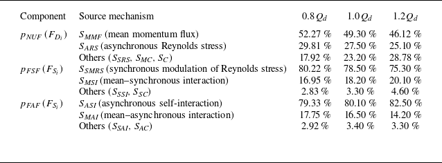
The quantitative results for all three pressure components ( $p_{\textit{NUF}}, p_{\textit{FSF}}, p_{\textit{FAF}}$ ) and their constituent sources are summarised in table 2. A consistent hierarchy of physical mechanisms is observed across the entire operating range. For the kinematic $p_{\textit{NUF}}$ component, the mean momentum flux ( $S_{\textit{MMF}}$ ) remains the primary driver, contributing between 46.12 % and 52.27 % to the local pressure asymmetry. The synchronous modulation of Reynolds stress ( $S_{\textit{SMRS}}$ ) consistently governs the dynamic $p_{\textit{FSF}}$ component with a dominant share of 75–80 %, while the asynchronous self-interaction ( $S_{\textit{ASI}}$ ) remains the principal source for the broadband $p_{\textit{FAF}}$ fluctuations.

Table 2.

Comparison of the contribution factors for $p_{\textit{NUF}}$ , $p_{\textit{FSF}}$ and $p_{\textit{FAF}}$ across different operating conditions.

Figure 16.

Spatial distribution of the NIP between source components: (a) NIP between $p_{\textit{NUF}}$ and $p_{\textit{FSF}}$ sources; (b) NIP between $p_{\textit{NUF}}$ and $p_{\textit{FAF}}$ sources. The scale identifies hotspots of physical coupling, highlighting the TLV as the common physical nexus for all components.

The systematic variations in the contribution factors further highlight the model's diagnostic utility. As the flow rate increases from $0.8Q_{{d}}$ to $1.2Q_{{d}}$ , the relative importance of $S_{\textit{MMF}}$ for $p_{\textit{NUF}}$ slightly decreases. This reflects the physical reality that at higher flow rates, the inflow becomes more aligned with the blade geometry, leading to a more uniform momentum flux distribution. Conversely, the centrifugal effect ( $S_{{C}}$ ) exhibits a relative increase in its contribution to pressure asymmetry as loading-related sources weaken. The high degree of consistency in the mechanism hierarchy indicates that the triple source model captures the fundamental, invariant features of turbomachinery unsteadiness while remaining responsive to changes in the operating state.

To address the underlying physical connection between the decomposed sources, a spatial correlation analysis based on the normalised intensity product (NIP) is performed. The NIP is defined as the product of the local source magnitudes normalised by their respective spatial means:

(4.8) \begin{equation} {\textit{NIP}}_{A,B}(\boldsymbol{x}) = \frac {|S_A(\boldsymbol{x})|}{\langle |S_A| \rangle } \times \frac {|S_B(\boldsymbol{x})|}{\langle |S_B| \rangle }. \end{equation}

This metric identifies hotspots where different mechanisms simultaneously exert high-intensity forcing on the pressure field.

Figure 16 displays the NIP maps between the kinematic source ( $p_{\textit{NUF}}$ ) and the two dynamic sources ( $p_{\textit{FSF}}$ and $p_{\textit{FAF}}$ ). A striking spatial co-location is observed: the coupling hotspots are strictly localised along the trajectory of the TLV and within the high-shear layers near the shroud. Physically, these results demonstrate that although the triple source model mathematically partitions the signal, these components share a common physical nexus. The TLV acts as the primary engine that simultaneously generates the steady pressure footprint ( $p_{\textit{NUF}}$ ), triggers the phase-locked dynamic modulations ( $p_{\textit{FSF}}$ ), and energises the stochastic fluctuations ( $p_{\textit{FAF}}$ ). The near-perfect spatial congruence at the vortex core confirms that the observed shroud unsteadiness is a multifaceted manifestation of the same underlying vortex dynamics, justifying the use of the triple source model to diagnose the distinct impacts of a single coherent structure.