1 Introduction
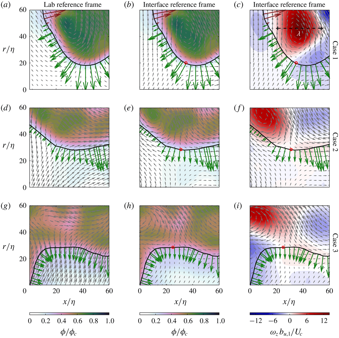
Turbulent entrainment describes the transport of unmixed or irrotational fluid across the jet boundary that separates the turbulent from the non-turbulent regions of the flow. The jet boundary can be characterised by an interfacial region known as the turbulent/non-turbulent interface, herein TNTI, whose finite thickness is of the order of the Taylor micro-scale and characterised by a jump in vorticity. The finite thickness of the TNTI also includes the viscous superlayer where the diffusion of vorticity occurs. Entrainment processes have wide-ranging implications in various scientific and engineering flow scenarios and it is therefore important to understand the mechanisms that influence the entrainment rates along the TNTI. Here we consider an axisymmetric turbulent jet in which the volume of the turbulent region grows downstream. From a time-averaged perspective, the growth of the jet is described by the classic entrainment hypothesis for which the jet entrains ambient fluid at a constant rate relative to a local velocity scale (Morton, Taylor & Turner Reference Morton, Taylor and Turner1956). However, from an instantaneous and local perspective, the jet entrains fluid elements from the non-turbulent region across the TNTI into the turbulent region and detrains fluid elements from the turbulent region into the non-turbulent region (Holzner & Lüthi Reference Holzner and Lüthi2011; Mistry et al.
Reference Mistry, Philip, Dawson and Marusic2016). As such, the velocity scale of interest is the local entrainment velocity,
 $\boldsymbol{V}$
, defined as the relative velocity between the surface propagation velocity of the TNTI,
 $\boldsymbol{u}_{s}$
, and the local fluid velocity at the interface,
 $\boldsymbol{u}_{I}$
, such that
 $\boldsymbol{V}=\boldsymbol{u}_{s}-\boldsymbol{u}_{I}$
. In the direction normal to the interface, denoted by the unit vector
 $\boldsymbol{n}$
,
 $\boldsymbol{V}=v_{n}\boldsymbol{n}$
, where the scalar quantity
 $v_{n}$
corresponds to the magnitude of the entrainment velocity normal to the TNTI.
Local entrainment or detrainment is described by the sign of the local normal entrainment velocity,
 $v_{n}$
, where
 $v_{n}\leqslant 0$
denotes entrainment and
 $v_{n}>0$
denotes detrainment. An expression for the entrainment velocity may be derived by first considering that the TNTI is identified by an isosurface of constant enstrophy (
 $\unicode[STIX]{x1D74E}^{2}$
) where the vorticity,
 $\unicode[STIX]{x1D74E}=\unicode[STIX]{x1D735}\times \boldsymbol{u}$
and
 $\boldsymbol{u}$
is the fluid velocity. The TNTI propagates according to
 $\unicode[STIX]{x2202}\unicode[STIX]{x1D74E}^{2}/\unicode[STIX]{x2202}t+\boldsymbol{u}_{s}\boldsymbol{\cdot }\unicode[STIX]{x1D735}\unicode[STIX]{x1D74E}^{2}=0,$
and in the normal direction,
 $\boldsymbol{n}=\unicode[STIX]{x1D735}\unicode[STIX]{x1D74E}^{2}/|\unicode[STIX]{x1D735}\unicode[STIX]{x1D74E}^{2}|$
. Substituting the term
 $\text{D}\unicode[STIX]{x1D74E}^{2}/\text{D}t$
using the enstrophy transport equation, Holzner & Lüthi (Reference Holzner and Lüthi2011) derived an equation for the magnitude of the entrainment velocity normal to the TNTI as:
 $$\begin{eqnarray}v_{n}=-\frac{2\unicode[STIX]{x1D714}_{i}\unicode[STIX]{x1D714}_{j}s_{ij}}{|\unicode[STIX]{x1D735}\unicode[STIX]{x1D74E}^{2}|}-\frac{\displaystyle \unicode[STIX]{x1D708}\frac{\unicode[STIX]{x2202}^{2}\unicode[STIX]{x1D714}^{2}}{\unicode[STIX]{x2202}x_{j}\unicode[STIX]{x2202}x_{j}}}{|\unicode[STIX]{x1D735}\unicode[STIX]{x1D74E}^{2}|}+\frac{\displaystyle 2\unicode[STIX]{x1D708}\left(\frac{\unicode[STIX]{x2202}\unicode[STIX]{x1D714}_{i}}{\unicode[STIX]{x2202}x_{j}}\right)^{2}}{|\unicode[STIX]{x1D735}\unicode[STIX]{x1D74E}^{2}|}.\end{eqnarray}$$
The terms on the right-hand side of this expression represent the contributions to
 $v_{n}$
from vortex stretching, diffusion and dissipation, respectively. In the viscous superlayer, the inviscid production term may be neglected (van Reeuwijk & Holzner Reference van Reeuwijk and Holzner2014), which leaves
 $v_{n}$
to be determined by the competing effects of viscous diffusion and dissipation. In a laminar flow, the expression for
 $v_{n}$
shows that only the latter two terms of (1.1) are present (see the Appendix in Philip et al. (Reference Philip, Bermejo-Moreno, Chung and Marusic2015)). An interesting and somewhat surprising result is that
 $v_{n}$
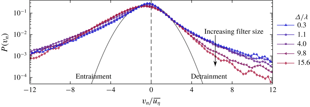
in a turbulent jet exhibits a broad probability density function (PDF)
 $P(v_{n})$
, see figure 4, and that the mean entrainment velocity (
 $\overline{v_{n}}$
) is an order of magnitude smaller than the instantaneous values of
 $v_{n}$
. We can decompose
 $\overline{v_{n}}=\int _{-\infty }^{\infty }P(v_{n})v_{n}\,\text{d}v_{n}=\int _{-\infty }^{0}P(v_{n})v_{n}\,\text{d}v_{n}+\int _{0}^{\infty }P(v_{n})v_{n}\,\text{d}v_{n}$
, where the first and second integrals correspond to entrainment and detrainment contributions to the mean respectively. Calculations based on figure 4 show that the mean entrainment is a result of about two parts of entrainment minus one part of detrainment. Thus, the exchange of fluid particles along the TNTI shows a characteristic imbalance between entrainment and detrainment reflected in a global growth rate of a turbulent axisymmetric jet.
In this paper we want to improve our understanding of the kinematics behind these processes. To do this we aim to address three broad questions: (i) How do local entrainment/detrainment rates in a high Reynolds number jet depend on the geometry of the TNTI, such as radial distance from the jet centreline and local curvature? (ii) Is there a characteristic turbulent structure that influences the local entrainment/detrainment velocity along the TNTI? (iii) Why do both entrainment and detrainment exhibit large magnitudes of
 $v_{n}$
(i.e. broad PDF of the entrainment velocity)? This is in contrast to a scenario where less entrainment and no detrainment might take place, and which still provides a net entrainment consistent with the jet growth. In answering these questions we reconcile our understanding of TNTI geometric features with the behaviour of the local entrainment velocity to achieve a description of the kinematics of the flow that improves or hinders the local entrainment rate.
Unravelling the structure of the TNTI has received considerable attention over the past two decades due to advances in experimental techniques and simulations. Beginning with Bisset, Hunt & Rogers (Reference Bisset, Hunt and Rogers2002), researchers have used reference frames aligned to the TNTI to extract an interface flow field description that cannot be achieved in the laboratory reference frame alone (Westerweel et al.
Reference Westerweel, Fukushima, Pedersen and Hunt2005, Reference Westerweel, Fukushima, Pedersen and Hunt2009; da Silva & Pereira Reference da Silva and Pereira2008; Taveira & da Silva Reference Taveira and da Silva2014; Chauhan, Philip & Marusic Reference Chauhan, Philip and Marusic2014a
; Chauhan et al.
Reference Chauhan, Philip, de Silva, Hutchins and Marusic2014b
; Gampert et al.
Reference Gampert, Boschung, Hennig, Gauding and Peters2014; Watanabe et al.
Reference Watanabe, Sakai, Nagata, Ito and Hayase2014a
; Borrell & Jiménez Reference Borrell and Jiménez2016; Mistry et al.
Reference Mistry, Philip, Dawson and Marusic2016). For example, an interface reference frame is necessary to reveal the steep jump-like profiles of vorticity and scalar concentration across the TNTI (Westerweel et al.
Reference Westerweel, Fukushima, Pedersen and Hunt2009; da Silva et al.
Reference da Silva, Hunt, Eames and Westerweel2014a
). Generally, it is understood that the thickness of the TNTI in mean-shear flows is characterised by the Taylor micro-scale
 $\unicode[STIX]{x1D706}$
(Westerweel et al.
Reference Westerweel, Fukushima, Pedersen and Hunt2005; da Silva & Taveira Reference da Silva and Taveira2010; Chauhan et al.
Reference Chauhan, Philip, de Silva, Hutchins and Marusic2014b
), whilst the wrinkled surface area of the interface is best described using a multi-scale fractal analysis (de Silva et al.
Reference de Silva, Philip, Chauhan, Meneveau and Marusic2013; Philip et al.
Reference Philip, Meneveau, de Silva and Marusic2014; Mistry et al.
Reference Mistry, Philip, Dawson and Marusic2016; Mistry, Dawson & Kerstein Reference Mistry, Dawson and Kerstein2018). Recent direct numerical simulations (DNS) of a planar shear layer and homogeneous isotropic turbulence by Silva, Zecchetto & da Silva (Reference Silva, Zecchetto and da Silva2018) have investigated the effect of higher Reynolds number on the characteristic thickness of the TNTI and found that the thickness scales with
 $\unicode[STIX]{x1D702}$
(and is of
 $O(10\unicode[STIX]{x1D702})$
) as opposed to a scaling with
 $\unicode[STIX]{x1D706}$
, although the thickness of the TNTI is close to
 $O(\unicode[STIX]{x1D706})$
. We acknowledge this may also apply to axisymmetric jets at high Reynolds number, however the measurements presented in this paper were not performed with the intention of resolving the inner structure of the TNTI and are therefore insufficient to verify
 $\unicode[STIX]{x1D702}$
-scaling.
Much of the recent work on the local entrainment velocity has focused on entrainment from a small-scale perspective, as first advocated by Corrsin & Kistler (Reference Corrsin and Kistler1955) and represents the final stage (‘mixing’) in a multi-stage entrainment process (Dimotakis Reference Dimotakis2005). Locally, viscous and molecular diffusion, also known as ‘nibbling’, are the dominant mechanisms by which vorticity and scalar concentration are transferred to non-turbulent fluid elements. For example, Holzner & Lüthi (Reference Holzner and Lüthi2011), Wolf et al. (Reference Wolf, Lüthi, Holzner, Krug, Kinzelbach and Tsinober2012, Reference Wolf, Lüthi, Holzner, Krug, Kinzelbach and Tsinober2013b
), van Reeuwijk & Holzner (Reference van Reeuwijk and Holzner2014), Watanabe et al. (Reference Watanabe, Sakai, Nagata, Ito and Hayase2014a
), Krug et al. (Reference Krug, Holzner, Lüthi, Wolf, Kinzelbach and Tsinober2015), Krug et al. (Reference Krug, Chung, Philip and Marusic2017) and Watanabe et al. (Reference Watanabe, Jaulino, Taveira, da Silva, Nagata and Sakai2017a
) have demonstrated that the diffusive (viscous) component of
 $v_{n}$
makes the greatest positive contribution to the local spreading of vorticity at the TNTI. By contrast, the inviscid contribution to
 $v_{n}$
is much smaller (Holzner & Lüthi Reference Holzner and Lüthi2011; Wolf et al.
Reference Wolf, Lüthi, Holzner, Krug, Kinzelbach and Tsinober2012, Reference Wolf, Holzner, Lüthi, Krug, Kinzelbach and Tsinober2013a
; Watanabe et al.
Reference Watanabe, Sakai, Nagata, Ito and Hayase2014a
).
Parenthetically, we note that the relatively minor contribution of inviscid terms to local
 $v_{n}$
described in the references above is not an argument to disregard the role of large-scale inviscid motions to net entrainment. Consider the net entrainment given by the expression
 $\int v_{n}\,\text{d}s=\overline{v_{n}}S$
, where
 $\text{d}s$
is the elemental length of the contorted surface area of the TNTI and
 $\overline{v_{n}}$
the average entrainment velocity that is
 $O\overline{u_{\unicode[STIX]{x1D702}}}$
, the Kolmogorov velocity. The influence of different length scales becomes evident if we spatially filter the field with a length scale
 $\unicode[STIX]{x1D6E5}$
, such that as
 $\unicode[STIX]{x1D6E5}$
becomes large we approach the mean field. It has been shown recently by Mistry et al. (Reference Mistry, Philip, Dawson and Marusic2016) in accordance with the original idea of Meneveau & Sreenivasan (Reference Meneveau and Sreenivasan1990) that
 $\overline{v_{n}}S=\overline{V}\overline{S}=V(\unicode[STIX]{x1D6E5})S(\unicode[STIX]{x1D6E5})$
, where
 $\overline{V}$
and
 $\overline{S}$
are the mean radial velocity and surface area, respectively, and
 $V(\unicode[STIX]{x1D6E5})$
,
 $S(\unicode[STIX]{x1D6E5})$
are the filtered values at the scale
 $\unicode[STIX]{x1D6E5}$
. Here,
 $\overline{V}\overline{S}$
is from the inviscid large-scale contributions (e.g. see Philip et al.
Reference Philip, Meneveau, de Silva and Marusic2014), which determines the overall entrainment rate. This is somewhat akin to the turbulent cascade process, where the rate of energy transfer is determined by the large-scale inviscid motion, and is equal to the net kinetic energy dissipation rate at the smallest scales through viscous motion. The analogy is further reinforced (Tritton Reference Tritton1988) when considering that the net axial momentum of a jet is constant, and that the velocity decays with downstream distance due to kinetic energy dissipation (as well as momentum distribution), which necessitates an increase in mass flux, i.e. a net entrainment into the jet across its boundary.
Researchers have often used the TNTI as a means to elicit features that influence the local entrainment rate. For example, the conditional local entrainment velocity is strongly linked to the local surface curvature (Wolf et al.
Reference Wolf, Lüthi, Holzner, Krug, Kinzelbach and Tsinober2012, Reference Wolf, Holzner, Lüthi, Krug, Kinzelbach and Tsinober2013a
; Philip et al.
Reference Philip, Bermejo-Moreno, Chung and Marusic2015; Jahanbakhshi & Madnia Reference Jahanbakhshi and Madnia2016; Watanabe et al.
Reference Watanabe, da Silva, Nagata and Sakai2017b
). Generally,
 $v_{n}$
is more negative (entrainment) along points where the TNTI curvature is convex towards the turbulent side, and
 $v_{n}$
is more positive (detrainment) along points where the curvature is concave. Additionally, there is some dependence of
 $v_{n}$
on orientation of the TNTI relative to the flow direction (Watanabe et al.
Reference Watanabe, Sakai, Nagata, Ito and Hayase2014a
), such as the leading or trailing edges of turbulent structures. Interestingly, Watanabe et al. (Reference Watanabe, Sakai, Nagata, Ito and Hayase2014b
), using their DNS of a planar jet, show that along the leading edges of the TNTI, the vorticity vector (which is usually parallel to the TNTI) is aligned with the stretching eigenvector direction of strain rate tensor, whereas the alignment of the vorticity vector is with the compression direction along the trailing edges of the TNTI. Ultimately, however, these studies are limited to comparing the local entrainment rate with another local flow quantity. To understand what turbulent structures are influencing the local entrainment rate we must consider the instantaneous flow field in the surrounding vicinity of the TNTI.
In this paper we implement a conditional-averaging technique in a reference frame aligned to the TNTI. The use of conditionally averaged profiles along radial coordinates or local normals to the TNTI have been used in many previous investigations (Bisset et al.
Reference Bisset, Hunt and Rogers2002; Westerweel et al.
Reference Westerweel, Fukushima, Pedersen and Hunt2009; da Silva & Taveira Reference da Silva and Taveira2010; Watanabe et al.
Reference Watanabe, Sakai, Nagata, Ito and Hayase2014a
; Chauhan et al.
Reference Chauhan, Philip, de Silva, Hutchins and Marusic2014b
). In contrast to these past studies, however, we apply conditioning of the local entrainment velocity,
 $v_{n}$
, on the geometric and flow features of the TNTI to elucidate the characteristics of the local flow field during entrainment and detrainment to compare them. In § 2 we introduce the experimental methods and techniques used to identify the TNTI and measure the local entrainment velocity along it. In § 3 we first characterise the entrainment velocity and features of the TNTI before identifying the coupling between them. Subsequently, in § 4 we evaluate mean profiles about the TNTI that are conditioned on the local entrainment velocity to compare the flow field during entrainment and detrainment, and try to identify the structure responsible for this. These findings are supported with instantaneous snapshots of the flow to qualitatively illustrate the role of Taylor micro-scale vortical structures in the local entrainment process. Finally, we summarise and conclude in § 5.
2 Experimental methods
We measured the velocity and scalar concentration fields across the radial–streamwise plane in the far field of an axisymmetric turbulent jet. The experiments were performed in a
 $7~\text{m}\times 1~\text{m}\times 1~\text{m}$
tank using water as the test medium and an aqueous solution of rhodamine 6G as the passive dye issued from a nozzle diameter
 $d=1$
cm. This provides an area ratio of the nozzle to tank of
 ${\approx}0.01\,\%$
, which is small enough to have negligible side wall effects. Furthermore, the jet was run for short durations to ensure no back flow and avoid the recirculation of dye back into the jet. The reproduction of classical scaling laws that we obtain in our jet as well as the PDF of
 $v_{n}$
we obtain (e.g. Mistry et al.
Reference Mistry, Philip, Dawson and Marusic2016) suggest that we have no noticeable effect of side walls and back flow. The Schmidt number of the scalar concentration field is
 $Sc\approx 8000$
(Crimaldi Reference Crimaldi2008). A separate reservoir was used to supply the turbulent jet with the dyed fluid and a series of pumps and valves ensured that a constant flow rate was maintained. This is confirmed with pressure measurements across an orifice plate. The Reynolds numbers of the jet are
 $Re=25\,300$
(
 $Re=u_{e}d/\unicode[STIX]{x1D708}$
) and
 $Re_{\unicode[STIX]{x1D706}}=260$
(
 $Re_{\unicode[STIX]{x1D706}}=\overline{u^{\prime 2}}^{1/2}\unicode[STIX]{x1D706}/\unicode[STIX]{x1D708}$
), where these symbols are defined in table 1. These Reynolds numbers are much higher than currently published works on local entrainment by other investigators (Holzner & Lüthi Reference Holzner and Lüthi2011; Wolf et al.
Reference Wolf, Lüthi, Holzner, Krug, Kinzelbach and Tsinober2012; Watanabe et al.
Reference Watanabe, Sakai, Nagata, Ito and Hayase2015). The streamwise, radial and spanwise coordinates are denoted by
 $x$
,
 $r$
and
 $z$
; corresponding velocities are denoted by
 $u$
,
 $v$
and
 $w$
, respectively. In this paper, we make use of a coordinate that is aligned to the TNTI contour which is denoted by
 $s$
.
Time, velocity and length scales of the turbulent jet. Quantities are measured along the jet centreline at a distance
 $50d$
downstream of the nozzle exit. The turbulence kinetic energy dissipation is defined as
 $\overline{\unicode[STIX]{x1D716}}=15\unicode[STIX]{x1D708}\overline{(\unicode[STIX]{x2202}u/\unicode[STIX]{x2202}x)^{2}}$
, the eddy turnover time is defined as
 ${\mathcal{T}}=b_{u,1/2}/U_{c}$
and the Taylor micro-scale is defined as
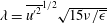 $\unicode[STIX]{x1D706}=\overline{{u^{\prime }}^{2}}^{1/2}\sqrt{15\unicode[STIX]{x1D708}/\overline{\unicode[STIX]{x1D716}}}$
and measured along the centreline at
 $x=50d$
.

Here we only provide a brief overview of the experimental measurement techniques as they are described in more detail in Mistry et al. (Reference Mistry, Philip, Dawson and Marusic2016, Reference Mistry, Dawson and Kerstein2018). Multi-scale particle image velocimetry (PIV) and planar laser-induced fluorescence (PLIF) measurements were taken about the
 $x/d=50$
streamwise location (
 $40<x/d<60$
) from the nozzle exit. This involved two high-speed PIV cameras measuring the particle fields at different resolutions and a single high-speed PLIF camera that captured the fluorescence of the passive dye. The field of view (FOV) of the coarse-resolution PIV and PLIF measurements is
 $200\times 200~\text{mm}^{2}$
and the vector spacing of this large-scale FOV (LFOV) PIV is
 $10\unicode[STIX]{x1D702}$
whilst the interrogation window size is
 $40\unicode[STIX]{x1D702}$
. An additional PIV camera was also used to measure the flow field with higher spatial resolution (small-scale FOV, SFOV), where the vector spacing is
 $3\unicode[STIX]{x1D702}$
. The scalar concentration fields were down-sampled to match the resolution of the PIV measurements. Spatial gradient quantities are evaluated using a least-squares differencing method (Raffel et al.
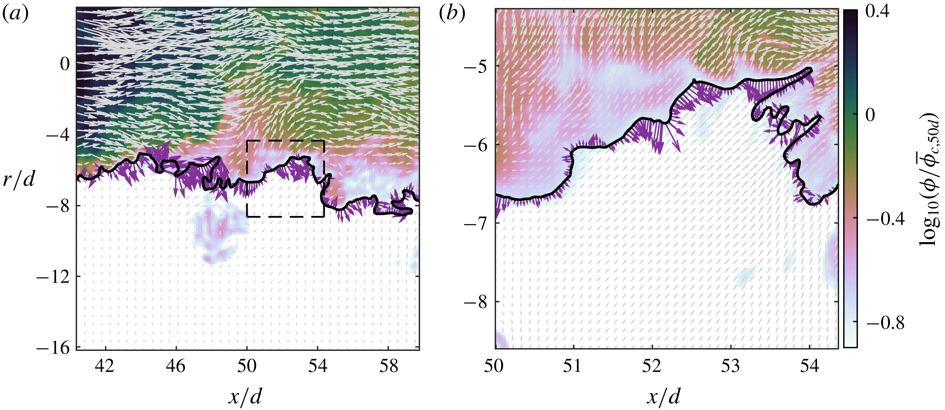
Reference Raffel, Willert, Wereley and Kompenhans1998). An example of the data captured with the PIV/PLIF set-up is presented in figure 1. The resultant data from the PIV and PLIF experiments yield
 $32\,724$
vector/scalar fields. Consecutive fields are spaced 1 ms apart, which is less than the Kolmogorov time scale,
 $\unicode[STIX]{x1D70F}_{\unicode[STIX]{x1D702}}\approx 11~\text{ms}$
, and hence capture the smallest temporal evolutions of the flow. However, we down-sample the fields to create a sample set of 1080 velocity/scalar fields that are spaced 30 ms (
 $3\unicode[STIX]{x1D70F}_{\unicode[STIX]{x1D702}}$
) apart for the calculation of mean statistics.
The instantaneous scalar concentration field in logarithmic scaling with the TNTI denoted by the black line, (a) LFOV and (b) SFOV. Instantaneous velocity vectors are superimposed in grey with every fourth velocity vector shown for clarity. Along the TNTI the local entrainment velocity,
 $\boldsymbol{V}$
, is plotted in purple. Note that the lengths of the purple
 $\boldsymbol{V}$
vectors and the grey velocity vectors are scaled differently. The dashed line box in (a) corresponds to the SFOV shown in (b).
2.1 Determination of the local entrainment velocity
Evaluating the local entrainment velocity,
 $\boldsymbol{V}=v_{n}\boldsymbol{n}$
, where
 $v_{n}$
is the magnitude of the entrainment velocity along the TNTI normal
 $\boldsymbol{n}$
, is a twofold procedure. It first requires a robust method to identify the TNTI and second the ability to track its motion in time. We only provide a brief description of the procedure as a detailed description can be found in Mistry et al. (Reference Mistry, Philip, Dawson and Marusic2016) and is similar to the ‘graphical’ approach of Wolf et al. (Reference Wolf, Lüthi, Holzner, Krug, Kinzelbach and Tsinober2012). We first identify the TNTI using isocontours of the scalar concentration field (
 $\unicode[STIX]{x1D719}$
) from a
 $Sc\gg 1$
passive scalar because planar velocity measurements cannot access the three-dimensional (3-D) vorticity field.
Following the approach of Prasad & Sreenivasan (Reference Prasad and Sreenivasan1989) and Westerweel et al. (Reference Westerweel, Hofmann, Fukushima and Hunt2002) we empirically identify a robust threshold value for scalar concentration that represents the TNTI. This is done by evaluating the conditional mean values of scalar concentration (
 $\unicode[STIX]{x1D719}$
), spanwise vorticity magnitude (
 $|\unicode[STIX]{x1D714}_{z}|$
), turbulence kinetic energy (
 $k$
) and axial velocity (
 $u$
) as a function of scalar concentration threshold,
 $\unicode[STIX]{x1D719}_{t}$
. For a given
 $\unicode[STIX]{x1D719}_{t}$
we extract all points that exceed the threshold value across all fields,
 $\unicode[STIX]{x1D719}>\unicode[STIX]{x1D719}_{t}$
. Ensemble averages are evaluated and the procedure repeated for a range of
 $\unicode[STIX]{x1D719}_{t}$
to construct profiles conditioned on the aforementioned variables. The inflection point of conditioned profiles coincides with the boundary of the turbulent field (Prasad & Sreenivasan Reference Prasad and Sreenivasan1989) which, in the current experiments, was determined to be
 $\unicode[STIX]{x1D719}/\unicode[STIX]{x1D719}_{c}=0.18$
, where
 $\unicode[STIX]{x1D719}_{c}$
is the local mean centreline scalar concentration. The TNTI is then identified by selecting the longest continuous isocontour of
 $\unicode[STIX]{x1D719}/\unicode[STIX]{x1D719}_{c}=0.18$
, an example of which is shown in figure 1 (thick black lines).
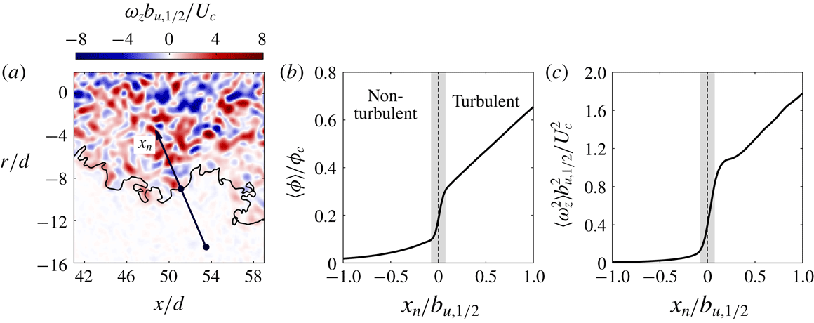
Conditionally averaged profiles are assembled in a frame of reference aligned with the TNTI in figure 2. This is done using an interface-normal vector
 $\boldsymbol{n}=(\unicode[STIX]{x1D735}\unicode[STIX]{x1D719}/|\unicode[STIX]{x1D735}\unicode[STIX]{x1D719}|)_{I}$
to generate an interface-normal coordinate
 $x_{n}$
(see figure 2
a), where subscript
 $I$
represents points along the TNTI. Note that the definition of
 $\boldsymbol{n}$
from now onwards is based on the isosurface of concentration rather than enstrophy that was used to obtain (1.1). We interpolate flow quantities onto
 $x_{n}$
using a bilinear interpolation scheme then ensemble average the data at the same normalised distance
 $x_{n}/b_{u,1/2}$
from each point along the instantaneous TNTI. Averaged quantities along
 $x_{n}$
are denoted by
 $\langle {\sim}\rangle$
. In some instances, the interface-normal coordinate may cross another point along the TNTI; this results in another transition from turbulent to non-turbulent fluid or vice versa. These points are discarded and only the points from the origin of
 $x_{n}$
up to the first crossing of the TNTI are considered. We do not consider the tangential coordinates because gradients along the interface are significantly smaller than the normal gradients (Philip et al.
Reference Philip, Meneveau, de Silva and Marusic2014). The smallest data spacing is selected to match the vector spacing in the LFOV PIV measurements and spans
 $x_{n}=0\pm b_{u,1/2}$
from the TNTI. The use of the local jet half-width,
 $b_{u,1/2}$
, ensures that the corresponding points along the
 $x_{n}$
-coordinate collapse across all measured TNTI positions.
(a) Instantaneous out-of-plane vorticity field
 $\unicode[STIX]{x1D714}_{z}$
normalised by the jet half-width
 $b_{u,1/2}$
and the mean centreline velocity
 $U_{c}$
. An example of the interface-normal coordinate
 $x_{n}$
is denoted by the black vector. (b) Mean conditionally averaged profile of scalar concentration along
 $x_{n}$
. The turbulent region is defined as
 $x_{n}>0$
and the non-turbulent region is defined as
 $x_{n}<0$
. The filled grey region represents the span across which the jump in scalar concentration occurs. (c) As for (b) but with the approximated enstrophy field
 $\unicode[STIX]{x1D714}_{z}^{2}$
.
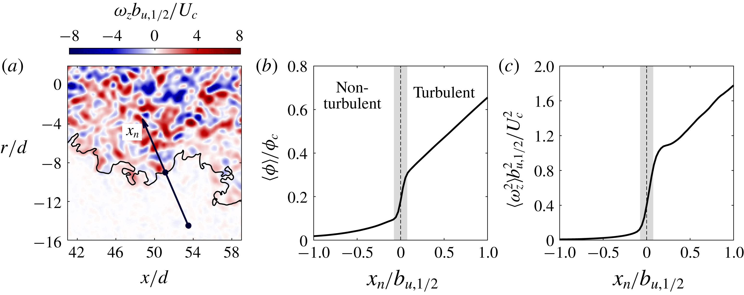
Figure 2(b,c) illustrates the jump profiles for
 $\langle \unicode[STIX]{x1D719}\rangle$
and
 $\langle \unicode[STIX]{x1D714}_{z}^{2}\rangle$
across the TNTI. These profiles, in addition to various other studies, establish that the observed jump in concentration in a
 $Sc\gg 1$
passive scalar field is well correlated with the jump in vorticity and enstrophy across the TNTI (Westerweel et al.
Reference Westerweel, Fukushima, Pedersen and Hunt2009; Watanabe et al.
Reference Watanabe, Sakai, Nagata, Ito and Hayase2015; Mistry et al.
Reference Mistry, Philip, Dawson and Marusic2016). We emphasise that the TNTI is composite in nature with a finite characteristic thickness of the order of the Taylor micro-scale which contains the viscous superlayer and whose outer boundary is identified by low values of vorticity and concentration that are challenging to resolve experimentally.
Schematic depicting the motion of the TNTI (red) between two points in time. The total motion of the TNTI between times
 $t_{0}$
(a) and
 $t_{0}+\text{d}t$
,
 $\boldsymbol{u}_{s}$
, comprises the advection (
 $\boldsymbol{u}_{I}$
) from the local fluid motion and the motion due to the local entrainment (
 $\boldsymbol{V}=v_{n}\boldsymbol{n}$
).

To evaluate
 $v_{n}$
, the motion of the TNTI needs to be decomposed into components of advection and entrainment, which is demonstrated in figure 3. Consider the motion of the TNTI over a short time interval from
 $t_{0}$
to time
 $t_{0}+\text{d}t$
. The TNTI will have moved due to (i) advection by the local fluid velocity,
 $\boldsymbol{u}_{I}$
and (ii) the growth of the turbulent region due to entrainment
 $\boldsymbol{V}=v_{n}\boldsymbol{n}$
. The local entrainment velocity at the TNTI is
 $\boldsymbol{V}=\boldsymbol{u}_{s}-\boldsymbol{u}_{I}$
. Simultaneous time-resolved measurements of the velocity and scalar fields enable us to carry out this procedure. This is done by displacing the interface at
 $t_{0}+\text{d}t$
by distance
 $-\boldsymbol{u}_{I}\,\text{d}t$
, where
 $\boldsymbol{u}_{I}$
is the local fluid velocity interpolated along the interface using a bilinear interpolation scheme. The local entrainment velocity,
 $v_{n}$
, is obtained by considering the local normal distance (
 $\text{d}\ell \boldsymbol{n}$
) from the interface at
 $t_{0}$
to the advection-subtracted interface,
 $v_{n}=\text{d}\ell /\text{d}t$
. The interface normals along the TNTI are pointing into the turbulent region, and therefore entrainment leads to the growth of the turbulent region and corresponds to a negative value,
 $v_{n}\leqslant 0$
, whereas detrainment corresponds to a shrinking of the turbulent region and a positive
 $v_{n}$
.
Previously (Mistry et al.
Reference Mistry, Philip, Dawson and Marusic2016) we applied this interface tracking technique and showed that the integral of the local entrainment velocities along the TNTI equals the global time-averaged entrainment rate demonstrating that the interface-tracking technique does not require spatial resolution down to the Kolmogorov or Bachelor length scale (
 $\unicode[STIX]{x1D702}$
) to recover the correct entrainment rate. Since we do not resolve the Kolmogorov and Batchelor scales we cannot assess whether the correlation between the jump in vorticity and scalar concentration will hold. However, additional support for the current approach is provided by Watanabe et al. (Reference Watanabe, Sakai, Nagata, Ito and Hayase2015) who recently investigated the Schmidt number dependence between the scalar concentration field and the local turbulent mixing across the viscous superlayer and the so-called turbulent sublayer. They show that the jump in scalar concentration occurs within the finite region of the TNTI for all Schmidt numbers,
 $Sc$
, evaluated (see their figure 7a) and when
 $\text{Sc}\gg 1$
, the jump in scalar concentration occurs in the turbulent sublayer providing a robust marker for the boundary between regions of high and low vorticity.
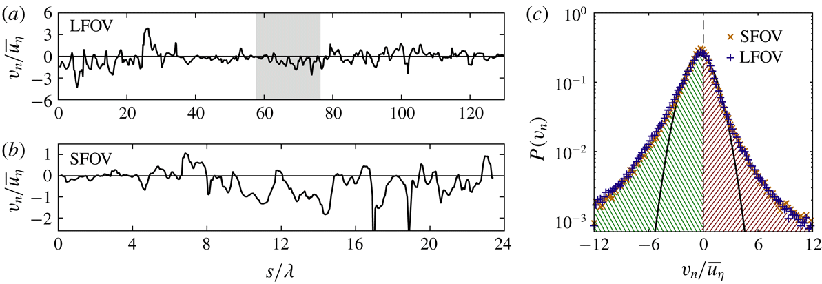
A sample instantaneous entrainment velocity profile measured along the TNTI for the LFOV (a) and SFOV (b). The coordinate
 $s$
is measured along the length of the TNTI. The grey region in the LFOV profile represents the equivalent region of the TNTI captured by the SFOV camera. (c) PDFs of the entrainment velocity for the LFOV (blue
 $+$
symbols) and SFOV data (orange
 $\times$
symbols). The thick black line indicates a Gaussian fit to
 $P(v_{n})$
for the LFOV data. Negative
 $v_{n}$
is defined as entrainment (green hatched region) and positive
 $v_{n}$
is defined as detrainment (red hatched region).

3 Statistical features of the entrainment velocity and the TNTI
3.1 Characteristics of the entrainment velocity
In this section we investigate the statistical characteristics of
 $v_{n}$
before considering conditional statistics of
 $v_{n}$
as a function of the local geometry of the TNTI. In figure 4(a,b) we present examples of instantaneous entrainment velocity profiles along the TNTI. The instantaneous
 $v_{n}$
signals along the TNTI are non-Gaussian, as evidenced by the intermittency of the profiles. The entrainment velocity is of the order of the mean Kolmogorov velocity,
 $\overline{u_{\unicode[STIX]{x1D702}}}$
, measured along the jet centreline at
 $x=50d$
. There are locations along the TNTI in which
 $v_{n}$
is typically around zero (see
 $40<s/\unicode[STIX]{x1D706}<60$
for LFOV), and other more compact sections where there is greater entrainment
 $v_{n}<-\overline{u_{\unicode[STIX]{x1D702}}}$
(noting the convention that negative
 $v_{n}$
corresponds to positive entrainment); for example see
 $0<s/\unicode[STIX]{x1D706}<20$
for LFOV. Similar behaviour is also observed in the SFOV shown in figure 4(b) which corresponds to the greyed region in (a).
The PDFs of
 $v_{n}$
for both the LFOV and SFOV are presented in figure 4(c). The distribution of
 $v_{n}$
is non-Gaussian, as made evident by the wide tails of the PDF compared to the Gaussian fit (black line), and is also qualitatively similar to the PDFs of
 $v_{n}$
for a range of turbulent flows (Holzner & Lüthi Reference Holzner and Lüthi2011; Wolf et al.
Reference Wolf, Lüthi, Holzner, Krug, Kinzelbach and Tsinober2012; Watanabe et al.
Reference Watanabe, Sakai, Nagata, Ito and Hayase2014a
; Krug et al.
Reference Krug, Holzner, Lüthi, Wolf, Kinzelbach and Tsinober2015). The mean value of the entrainment velocity along the TNTI measured from the LFOV data is
 $-\overline{v_{n}}=0.68\overline{u_{\unicode[STIX]{x1D702}}}$
, which is comparable to the results of Wolf et al. (Reference Wolf, Lüthi, Holzner, Krug, Kinzelbach and Tsinober2012), who report that
 $-\overline{v_{n}}\approx 0.7\overline{u_{\unicode[STIX]{x1D702}}}$
for an axisymmetric jet at
 $Re=5000$
, and also van Reeuwijk & Holzner (Reference van Reeuwijk and Holzner2014), who report that
 $0<-\overline{v_{n}}<\overline{u_{\unicode[STIX]{x1D702}}}$
for DNS of a temporal jet. However, it has been previously demonstrated in Mistry et al. (Reference Mistry, Philip, Dawson and Marusic2016) that
 $\overline{v_{n}}$
is dependent on the measurement resolution and follows a power-law scaling
 $-\overline{v_{n}}\sim \unicode[STIX]{x1D6E5}^{0.31}$
, where
 $\unicode[STIX]{x1D6E5}$
is the spatial resolution (or the filter size in a multi-scale analysis). In the limit of
 $\unicode[STIX]{x1D6E5}$
becoming large (of the order of the jet width), the mean entrainment velocity approaches the bulk entrainment velocity obtained from the entrainment hypothesis (Turner Reference Turner1986). Nevertheless, this resolution dependence of
 $\overline{v_{n}}$
does not change the general conclusion that the local entrainment velocity along the TNTI is non-Gaussian and has a non-zero, albeit small mean value (
 $-\overline{v_{n}}\sim \overline{u_{\unicode[STIX]{x1D702}}}$
), as first hypothesised by Corrsin & Kistler (Reference Corrsin and Kistler1955). At this point it is worth reiterating that the mean
 $\overline{v_{n}}=\int _{-\infty }^{\infty }P(v_{n})v_{n}\,\text{d}v_{n}=-0.68\overline{u_{\unicode[STIX]{x1D702}}}$
has a contribution from both entrainment (
 $\int _{-\infty }^{0}P(v_{n})v_{n}\,\text{d}v_{n}=-1.19\overline{u_{\unicode[STIX]{x1D702}}}$
) as well as from detrainment (
 $\int _{0}^{\infty }P(v_{n})v_{n}\,\text{d}v_{n}=0.51\overline{u_{\unicode[STIX]{x1D702}}}$
). This ratio of approximately two parts of entrainment for one part of detrainment is in good agreement with the viscous superlayer model derived by van Reeuwijk & Holzner (Reference van Reeuwijk and Holzner2014), as well as the laminar calculations of Philip et al. (Reference Philip, Bermejo-Moreno, Chung and Marusic2015) where the
 $2:1$
ratio of
 $\text{entrainment}:\text{detrainment}$
can be obtained analytically. It is therefore necessary to investigate both entrainment and detrainment rates for a fuller understanding of the overall entrainment rate.
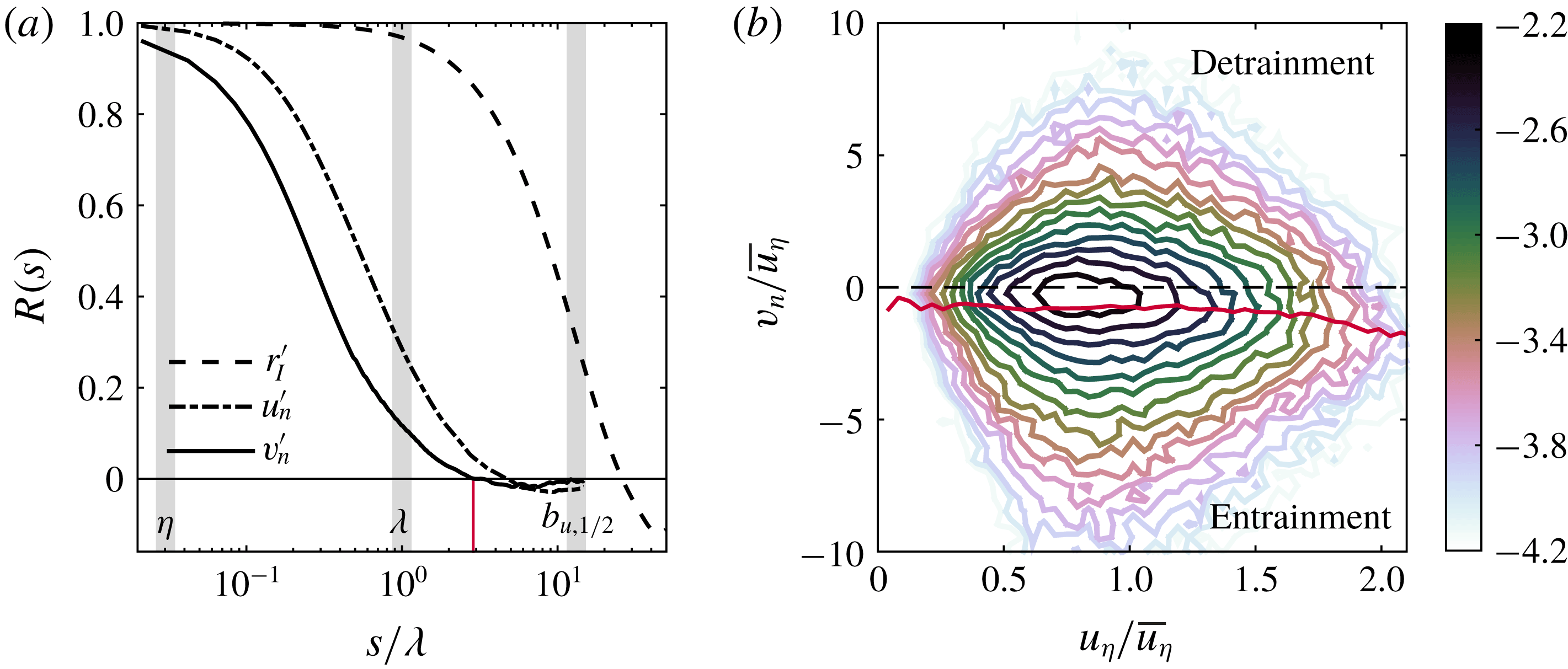
(a) The auto-correlation functions of the entrainment velocity (
 $R_{v_{n}^{\prime }v_{n}^{\prime }}$
, solid line), interface-normal velocity (
 $R_{u_{n}^{\prime }u_{n}^{\prime }}$
, dash-dot line) and the radial position of the TNTI (
 $R_{r_{I}^{\prime }r_{I}^{\prime }}$
, dashed line) in logarithmic scaling. The vertical grey bars denote the Kolmogorov length scale (
 $\unicode[STIX]{x1D702}$
), Taylor micro-scale (
 $\unicode[STIX]{x1D706}$
) and the jet half-width (
 $b_{u,1/2}$
) from left-to-right, respectively. (b) Joint PDF of the entrainment velocity,
 $v_{n}$
, and the local Kolmogorov velocity,
 $u_{\unicode[STIX]{x1D702}}=(\unicode[STIX]{x1D708}\unicode[STIX]{x1D716}_{loc})^{1/4}$
, along the TNTI. Note that
 $\unicode[STIX]{x1D716}_{loc}$
represents the approximation to the local dissipation rate
 $\unicode[STIX]{x1D716}_{loc}=15\unicode[STIX]{x1D708}(\unicode[STIX]{x2202}u/\unicode[STIX]{x2202}x)^{2}$
, whereas the mean dissipation along the jet centreline is denoted as
 $\overline{\unicode[STIX]{x1D716}}$
. The colour bar shows the logarithm of the joint PDF.
Given the presence of both entrainment and detrainment along the TNTI, we now evaluate the characteristic length scale of these features. Westerweel et al. (Reference Westerweel, Fukushima, Pedersen and Hunt2005) and Chauhan et al. (Reference Chauhan, Philip, de Silva, Hutchins and Marusic2014b
) determine the characteristic length scale of the TNTI by evaluating the auto-correlation function of axial velocity (
 $u^{\prime }$
) and interface-normal velocity fluctuations (
 $u_{n}^{\prime }$
), respectively. Here we have access to the local entrainment rate along the TNTI and can therefore directly measure the auto-correlation function of
 $v_{n}$
to identify the characteristic length scale of the local entrainment process. In figure 5(a) we present the auto-correlation function of the entrainment velocity,
 $R_{v_{n}^{\prime }v_{n}^{\prime }}(s)$
for the SFOV dataset. Here
 $v_{n}^{\prime }$
is the fluctuating entrainment velocity defined as
 $v_{n}^{\prime }=v_{n}-\overline{v_{n}}$
. We integrate
 $R_{v_{n}^{\prime }v_{n}^{\prime }}(s)$
to determine the characteristic entrainment length scale and for simplicity we only integrate up to the zero crossing of the correlation function. This gives a characteristic entrainment length scale of
 $0.48\unicode[STIX]{x1D706}$
, which is
 $O(\unicode[STIX]{x1D706})$
, and emphasises the role of
 $\unicode[STIX]{x1D706}$
-sized structures in the local entrainment process. This is also comparable to the thickness of the of the TNTI in free-shear flows which is of
 $O(\unicode[STIX]{x1D706})$
(Westerweel et al.
Reference Westerweel, Fukushima, Pedersen and Hunt2005; da Silva & Taveira Reference da Silva and Taveira2010; Chauhan et al.
Reference Chauhan, Philip and Marusic2014a
). Interestingly, we observe that the correlation function becomes negative at distance of
 $s=2.9\unicode[STIX]{x1D706}$
(see red line), which indicates that the local entrainment alternates between high and low entrainment rates at length scales of the order of the Taylor micro-scale. For comparison, we also evaluate the auto-correlation function of the interface-normal velocity fluctuations (
 $u_{n}^{\prime }$
, see figure 5
a, dash-dot line) to compare with Westerweel et al. (Reference Westerweel, Fukushima, Pedersen and Hunt2005) and Chauhan et al. (Reference Chauhan, Philip, de Silva, Hutchins and Marusic2014b
). The interface-normal velocity is determined by the dot product of the local fluid velocity along the TNTI and the local interface-normal unit vector,
 $u_{n}=\boldsymbol{u}_{I}\boldsymbol{\cdot }\boldsymbol{n}$
, and the fluctuating component is
 $u_{n}^{\prime }=u_{n}-\overline{u_{n}}$
. The characteristic length scale of
 $u_{n}^{\prime }$
is determined to be
 $0.86\unicode[STIX]{x1D706}$
, which is comparable to the entrainment velocity,
 $O(\unicode[STIX]{x1D706})$
, and consistent with Westerweel et al. (Reference Westerweel, Fukushima, Pedersen and Hunt2005) and Chauhan et al. (Reference Chauhan, Philip, de Silva, Hutchins and Marusic2014b
).
The auto-correlation function of the radial distance from the jet centreline to the TNTI,
 $R_{r_{I}^{\prime }r_{I}^{\prime }}(s)$
, is also plotted figure 5(a). A comparison with
 $R_{v_{n}^{\prime }u_{v}^{\prime }}$
and
 $R_{u_{n}^{\prime }u_{n}^{\prime }}$
, shows that the radial position of the TNTI remains correlated over longer distances that are of the order of the jet half-width,
 $0.77b_{u,1/2}$
or equivalently
 $10.1\unicode[STIX]{x1D706}$
. A length scale
 $L_{r_{I}}=O(b_{u,1/2})$
is also in agreement with observations in a turbulent boundary layer (Chauhan et al.
Reference Chauhan, Philip, de Silva, Hutchins and Marusic2014b
) where the TNTI remains correlated over distances of the order of the boundary layer thickness,
 $O(\unicode[STIX]{x1D6FF})$
(i.e. the largest characteristic length scale). The correlation of
 $R_{r_{I}^{\prime }r_{I}^{\prime }}(s)$
is a footprint of large-scale undulations of the TNTI which, in combination with the small-scale wrinkling of the TNTI observed in figure 1, demonstrates the multi-scale modulation of the TNTI surface area (Sreenivasan, Ramshankar & Meneveau Reference Sreenivasan, Ramshankar and Meneveau1989; de Silva et al.
Reference de Silva, Philip, Chauhan, Meneveau and Marusic2013; Chauhan et al.
Reference Chauhan, Philip, de Silva, Hutchins and Marusic2014b
; Mistry et al.
Reference Mistry, Philip, Dawson and Marusic2016).
An earlier study in a shear-free flow by Holzner & Lüthi (Reference Holzner and Lüthi2011) showed that along the TNTI
 $v_{n}$
is independent of
 $u_{\unicode[STIX]{x1D702}}$
, and therefore the local dissipation field (see their figure 4). The implication is that the local mass flux across the TNTI is not strongly influenced by the local small-scale turbulence. We present evidence that this is also the case for a free-shear flow at high Reynolds number in figure 5(b). Here we show the joint PDF (J-PDF) of the local entrainment velocity and the local Kolmogorov velocity,
 $u_{\unicode[STIX]{x1D702}}=(\unicode[STIX]{x1D708}\unicode[STIX]{x1D716}_{loc})^{1/4}$
, where the local dissipation rate is approximated by
 $\unicode[STIX]{x1D716}_{loc}=15\unicode[STIX]{x1D708}(\unicode[STIX]{x2202}u/\unicode[STIX]{x2202}x)^{2}$
at each point along the TNTI. Superimposed on this plot in red is the conditional mean entrainment velocity for a given value of
 $u_{\unicode[STIX]{x1D702}}$
,
 $\overline{v_{n}}|_{u_{\unicode[STIX]{x1D702}}}$
. (We will have further comments on this in § 3.3.) No discernible variation of
 $\overline{v_{n}}|_{u_{\unicode[STIX]{x1D702}}}$
with changing
 $u_{\unicode[STIX]{x1D702}}$
is observed, which suggests that locally, there is no strong correlation between the turbulent dissipation and diffusion of vorticity.
3.2 Geometric characteristics of the TNTI
In this section we provide statistical characterisation of the TNTI geometry, and although some of these results are known from the TNTI analysis of other flows they are included here because, (i) such properties are not known for a high-
 $Re$
jet, and (ii) more importantly, they are employed in the next section to investigate conditional statistics of
 $v_{n}$
. In particular, we focus on the radial distance from the centreline to the TNTI,
 $r_{I}$
, the interface curvature,
 $\unicode[STIX]{x1D705}$
, and the interface orientation,
 $\unicode[STIX]{x1D703}$
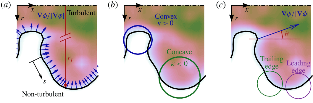
. The radial position of the interface,
 $r_{I}$
, is the distance along the radial axis from the jet centreline to the local position of the TNTI, as shown in figure 6(a). The interface curvature
 $\unicode[STIX]{x1D705}$
represents the rate of change of the interface direction, and is evaluated in two dimensions using the following parametric expression:
 $$\begin{eqnarray}\unicode[STIX]{x1D705}=\frac{\displaystyle \frac{\text{d}x}{\text{d}s}\frac{\text{d}^{2}r}{\text{d}s^{2}}-\frac{\text{d}r}{\text{d}s}\frac{\text{d}^{2}x}{\text{d}s^{2}}}{\displaystyle \left[\left(\frac{\text{d}x}{\text{d}s}\right)^{2}+\left(\frac{\text{d}r}{\text{d}s}\right)^{2}\right]^{3/2}}.\end{eqnarray}$$
Figure 6(b) illustrates the definition of convex (
 $\unicode[STIX]{x1D705}>0$
) and concave (
 $\unicode[STIX]{x1D705}<0$
) curvatures of the TNTI. The orientation of the TNTI,
 $\unicode[STIX]{x1D703}$
, is measured as the angle between the streamwise axis,
 $x$
, and the local interface-normal unit vector along the TNTI,
 $\boldsymbol{n}$
. The angular range
 $90^{\circ }\leqslant \unicode[STIX]{x1D703}\leqslant 180^{\circ }$
represents the ‘leading edge’ of the interface, and
 $0^{\circ }\leqslant \unicode[STIX]{x1D703}<90^{\circ }$
represents the ‘trailing edge’. Examples of the TNTI leading edge and trailing edge are highlighted in figure 6(c) by the purple and green circles, respectively. We evaluate the aforementioned features at each point along the TNTI and for each of the 1080 realisations of the flow.
Schematic of the geometric features of the TNTI: (a) the interface-normal unit vectors,
 $\boldsymbol{n}=(\unicode[STIX]{x1D735}\unicode[STIX]{x1D719}/|\unicode[STIX]{x1D735}\unicode[STIX]{x1D719}|)_{I}$
, the interface radial position,
 $r_{I}$
, and the coordinate along the TNTI,
 $s$
; (b) the interface curvature,
 $\unicode[STIX]{x1D705}$
; and (c) the interface angle (measured to the local normal shown in blue),
 $\unicode[STIX]{x1D703}$
. The filled contours represents the instantaneous scalar concentration field,
 $\unicode[STIX]{x1D719}$
, and the thick black line represents the TNTI.

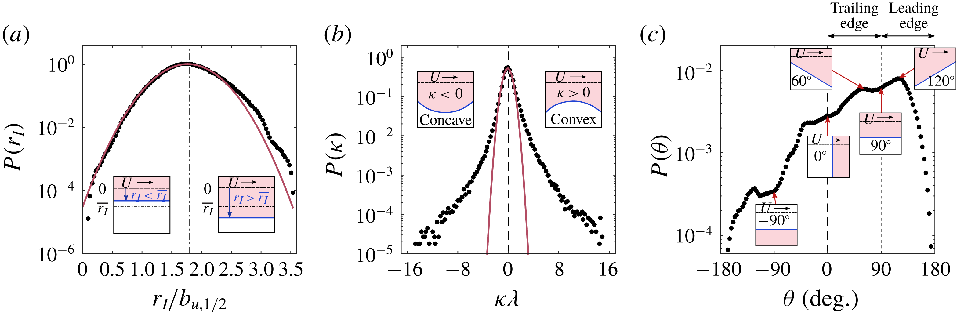
The PDFs of (a) interface radial position
 $r_{I}$
, (b) interface curvature
 $\unicode[STIX]{x1D705}$
and (c) orientation of the interface normal from the centreline
 $\unicode[STIX]{x1D703}$
. Gaussian fits to the PDFs are shown in red. The mean radial position,
 $\overline{r_{I}}=1.79b_{u,1/2}$
, is denoted by the black dash-dot line in (a). The inset plots depict the geometric features of the interface, where the dark (blue) line is the TNTI, and the pink fill denotes the turbulent region. Similar insets are presented in figure 8 for convenience.
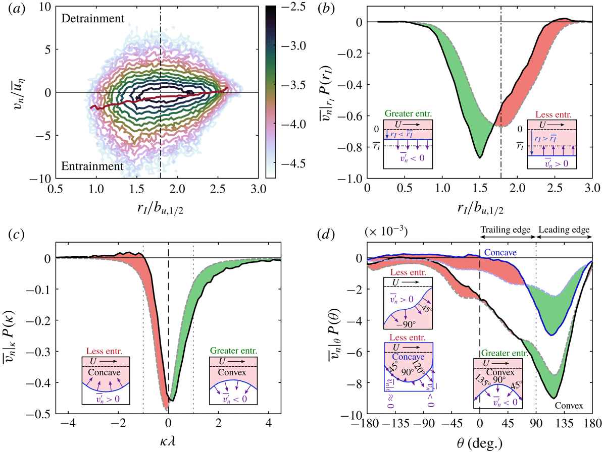
(a) J-PDF of the entrainment velocity as a function of radial position
 $r_{I}$
with the conditional mean entrainment velocity
 $\overline{v_{n}}|_{r_{I}}$
denoted by the red line. (b–d) Conditional mean entrainment velocity weighted by the local probability of the independent variables presented in figure 7 (
 $\overline{v_{n}}|_{f}P(f)$
, thick solid lines): (b) radial position
 $r_{I}$
, (c) interface curvature
 $\unicode[STIX]{x1D705}$
and (d) interface orientation
 $\unicode[STIX]{x1D703}$
. The product of the (unconditioned) mean entrainment velocity,
 $\overline{v_{n}}$
, and the probability of the independent variables is denoted by the dashed lines,
 $\overline{v_{n}}P(f)$
.

Figure 7 presents the PDFs of the geometric characteristics of TNTI; Gaussian profiles fitted to the distributions are shown in red. The PDF of the TNTI radial position is presented in figure 7(a) where
 $r_{I}$
is normalised by the local mean half-width of the jet,
 $b_{u,1/2}$
. Normalising
 $r_{I}$
in this manner yields a PDF distribution that collapses across a range of streamwise distances in an axisymmetric jet (Westerweel et al.
Reference Westerweel, Fukushima, Pedersen and Hunt2009; Mistry et al.
Reference Mistry, Philip, Dawson and Marusic2016). The distribution of
 $r_{I}$
is approximately Gaussian in agreement with the early predictions of Corrsin & Kistler (Reference Corrsin and Kistler1955) and with more recent results in a range of turbulent shear flows (Bisset et al.
Reference Bisset, Hunt and Rogers2002; Westerweel et al.
Reference Westerweel, Fukushima, Pedersen and Hunt2005; Chauhan et al.
Reference Chauhan, Philip, de Silva, Hutchins and Marusic2014b
). We note a slight asymmetry in the PDF distribution, which could be due to the jet flapping and/or convergence, and reasons are not completely clear.
The radial position of the TNTI spans several half-widths, which indicates that there are large-scale spatial fluctuations of the TNTI position. This is contrasted by the PDF of curvature in figure 7(b), which exhibits wide tails because of the presence of small-scale wrinkling along the interface. Evidence of these sharp contortions is also shown in the instantaneous TNTI example in figure 1.
The PDF of the interface orientation is presented in figure 7(c). For clarity the plot is annotated with illustrations of particular surface orientations; note that the pink fill denotes the turbulent region. The TNTI is most commonly oriented at an angle of
 $120^{\circ }$
, with a secondary peak at
 $60^{\circ }$
. These angles respectively fall within the leading (
 $90^{\circ }\leqslant \unicode[STIX]{x1D703}\leqslant 180^{\circ }$
) and trailing (
 $0^{\circ }\leqslant \unicode[STIX]{x1D703}<90^{\circ }$
) edge regions of the TNTI. The local minima near
 $90^{\circ }$
(i.e. parallel to streamwise axis,
 $x$
) suggests that the interface does not preferentially align with the jet axes. It is for this reason that in § 4 we consider the flow field in a frame of reference that is aligned to the TNTI rather than a laboratory frame of reference aligned to the jet coordinates.
3.3 Local entrainment and the TNTI
Given the TNTI geometric features identified in the previous section, we now evaluate the dependence of the local entrainment velocity on these geometric features. This is first illustrated in figure 8(a) by presenting the J-PDF between the local entrainment velocity
 $v_{n}$
and radial position
 $r_{I}$
of the TNTI. Given some value of
 $r_{I}$
, we also evaluate the conditional mean entrainment velocity,
 $$\begin{eqnarray}\overline{v_{n}}|_{r_{I}}=\frac{1}{P(r_{I})}\int P(v_{n},r_{I})v_{n}\,\text{d}v_{n}=\int P(v_{n}|r_{I})v_{n}\,\text{d}v_{n},\end{eqnarray}$$
which is the mean entrainment velocity for a given
 $r_{I}$
. This is illustrated by the solid (red) line in figure 8(a). From the J-PDF it is apparent that the local entrainment takes a wide range of values for any given radial position; however, the tilt in the
 $\overline{v_{n}}|_{r_{I}}$
line in figure 8(a) suggests that entrainment is common at smaller radial distances whereas there is a preference for detrainment further away from the centreline.
To quantify the contributions of different
 $r_{I}$
locations to the mean entrainment velocity, we now use the statistical features of
 $\overline{v_{n}}|_{r_{I}}$
. Here values of
 $\overline{v_{n}}|_{r_{I}}$
are weighted by the local probability
 $P(r_{I})$
of the conditioning variable. In general, we use
 $\overline{v_{n}}|_{f}P(f)$
, where
 $f$
is the conditioning variable, which could be
 $r_{I}$
,
 $\unicode[STIX]{x1D703}$
,
 $\unicode[STIX]{x1D705}$
, or any other variable. These are denoted by the thick solid black lines plotted in figure 8(b–d). It is understood that the area under the curve,
 $\int \overline{v_{n}}|_{f}P(f)\,\text{d}f=\overline{v_{n}}$
, is equal to the mean entrainment. For comparison, we include the product of the unconditioned mean entrainment velocity and the local probability of the independent variable,
 $\overline{v_{n}}P(f)$
, as dashed lines. If
 $v_{n}$
is independent of the variable
 $f$
then the profiles of
 $\overline{v_{n}}|_{f}P(f)$
and
 $\overline{v_{n}}P(f)$
would collapse. This approach enables us to determine when
 $\overline{v_{n}}|_{f}$
is smaller or larger than
 $\overline{v_{n}}$
, and therefore elicit the influence on entrainment from a specific geometric feature of the TNTI. For ease of interpretation we plot filled colours between the
 $\overline{v_{n}}|_{f}P(f)$
solid lines and
 $\overline{v_{n}}P(f)$
dashed lines in figure 8(b–d). The green filled area corresponds to the condition
 $\overline{v_{n}}|_{f}<\overline{v_{n}}$
(more negative), which means that there is greater entrainment for a given
 $f$
. Recall that negative
 $v_{n}$
denotes positive entrainment. Similarly, the red filled area corresponds to the condition where
 $\overline{v_{n}}|_{f}>\overline{v_{n}}$
, which means that the conditional entrainment velocity is more positive (less entrainment) for the given conditioning variable
 $f$
.
First consider the dependence of the entrainment velocity on the TNTI radial position in figure 8(b). The green area shows that greater entrainment occurs when the TNTI is closer to the centreline of the jet where there is greater streamwise momentum. Entrainment increases for radial positions less than the mean TNTI position
 $\overline{r_{I}}=1.79b_{u,1/2}$
whereas beyond
 $r_{I}\approx 2.5b_{u,1/2}$
the conditional mean entrainment velocity becomes positive. This indicates that at radial positions much greater than the mean the turbulent region detrains and the flow goes to a non-turbulent state. The radial dependence of
 $v_{n}$
highlights the importance of large-scale motions on entrainment because
 $r_{I}$
spans several jet half-widths (figure 7).
Figure 8(c) shows the dependence of entrainment velocity with local interface curvature. Entrainment is enhanced (green region) when the curvature is positive, convex to the turbulent region, and reduced (red region) when the TNTI curvature is negative, concave to the turbulent region. Along concave curvatures in the region
 $-3<\unicode[STIX]{x1D705}\unicode[STIX]{x1D706}<-1$
,
 $\overline{v_{n}}$
becomes positive, which means that the turbulent region is detraining on average. The dotted lines denote the limits
 $-\unicode[STIX]{x1D706}\leqslant \unicode[STIX]{x1D705}\leqslant \unicode[STIX]{x1D706}$
, which encapsulates 87 % of all points along the TNTI;
 $\unicode[STIX]{x1D705}<-\unicode[STIX]{x1D706}$
and
 $\unicode[STIX]{x1D705}>\unicode[STIX]{x1D706}$
account for 6 % and 7 % of points, respectively. This demonstrates that the bulk of local entrainment occurs alongside structures of
 $O(\unicode[STIX]{x1D706})$
or larger. These findings are in agreement with previous studies conducted at lower Reynolds numbers (Dopazo, Martin & Hierro Reference Dopazo, Martin and Hierro2007; Wolf et al.
Reference Wolf, Lüthi, Holzner, Krug, Kinzelbach and Tsinober2012, Reference Wolf, Holzner, Lüthi, Krug, Kinzelbach and Tsinober2013a
). It is important to note that planar measurements are limited to the principal curvature
 $k_{1}$
(Dopazo et al.
Reference Dopazo, Martin and Hierro2007) rather than the full 3-D surface curvature. Nonetheless, the component of curvature that we do capture is most likely to be shaped by the dominant streamwise shear (Bisset et al.
Reference Bisset, Hunt and Rogers2002).
The dependence of
 $\overline{v_{n}}$
conditioned on the TNTI surface orientation is depicted in figure 8(d). We apply additional conditioning of these profiles based on the local curvature. The entrainment velocity conditioned on TNTI orientation with negative curvature (concave) is denoted by the solid blue line for
 $\overline{v_{n}}|_{\unicode[STIX]{x1D703}|\unicode[STIX]{x1D705}<0}P(\unicode[STIX]{x1D703}|_{\unicode[STIX]{x1D705}<0})$
, and the light-blue dash-dot line for
 $\overline{v_{n}}|_{\unicode[STIX]{x1D705}<0}P(\unicode[STIX]{x1D703}|_{\unicode[STIX]{x1D705}<0})$
. The entrainment velocity conditioned on TNTI orientation with positive curvature (convex) is denoted by the solid black line for
 $\overline{v_{n}}|_{\unicode[STIX]{x1D703}|\unicode[STIX]{x1D705}>0}P(\unicode[STIX]{x1D703}|_{\unicode[STIX]{x1D705}>0})$
, and the grey dashed line for
 $\overline{v_{n}}|_{\unicode[STIX]{x1D705}>0}P(\unicode[STIX]{x1D703}|_{\unicode[STIX]{x1D705}>0})$
. This conditioning is more clearly illustrated by the inset schematics in figure 8(d). First consider the positive curvature profiles (black and grey lines): the conditional entrainment velocity is approximately 15 % more negative than the mean entrainment velocity in the range
 $70^{\circ }<\unicode[STIX]{x1D703}<135^{\circ }$
. Outside this region the conditional entrainment velocity is either equal to or less than the mean entrainment velocity. Thus, for convex curvatures the local entrainment velocity is only weakly dependent on the surface orientation. In contrast, there is much greater dependence on surface orientation for the concave (negative) curvature profiles (dark and light blue lines): at
 $\unicode[STIX]{x1D703}\approx 120^{\circ }$
the conditional entrainment velocity is 130 % more negative than the mean entrainment velocity for
 $\unicode[STIX]{x1D705}<0$
. Generally, for negative curvatures (concave) there is greater entrainment along leading edges and less entrainment along the trailing edges. The entrainment velocity also becomes positive (i.e. flow detrains) along concave curvatures where
 $\unicode[STIX]{x1D703}<0^{\circ }$
. These results support the work of Watanabe et al. (Reference Watanabe, Sakai, Nagata, Ito and Hayase2014a
) who also report that
 $v_{n}$
is largest along the leading edges of the TNTI and smallest along the trailing edges, but they do not evaluate the dependence on the local curvature. We show that the entrainment in regions of positive curvature (convex) is less dependent on the TNTI surface orientation, although overall more entrainment occurs in regions of convex curvature compared to concave curvature.
We may summarise the findings of figure 8 as follows: there is greater entrainment along the TNTI when the interface is nearer to the jet centreline. Entrainment is also enhanced by local curvature that is convex to the turbulent region. The entrainment velocity along convex surface curvatures is only weakly dependent on the local surface orientation of the TNTI. Along concave surface curvatures there is more positive entrainment along the leading edges of the TNTI, but also more detrainment elsewhere. These local entrainment findings are sketched in the inset plots of figure 8. It is also interesting that the conditional entrainment velocity is predominantly negative given that the PDF of
 $v_{n}$
in figure 4(c) shows only a slight skewness towards entrainment compared to detrainment. To better understand this conditional behaviour of
 $v_{n}$
we must now consider the kinematics of the flow about the TNTI, which ultimately generate these geometric features.
3.4 The conditional flow field along the TNTI
In this section we evaluate the conditional mean entrainment velocity,
 $v_{n}$
, as a function of the local fluid velocity along the TNTI with the aim of elucidating the kinematic features of local entrainment. We first consider the alignment between the local fluid velocity vector,
 $\boldsymbol{u}_{I}$
, and the local normal unit vector,
 $\boldsymbol{n}$
, defined by the cosine of the angle between them,
 $\cos (\unicode[STIX]{x1D713})$
, along the TNTI. This is illustrated in figure 9(a) which shows the unit vectors locally normal to the TNTI,
 $\boldsymbol{n}$
, (dark grey arrows) and the local fluid velocity
 $\boldsymbol{u}_{I}$
(red arrows).
The PDF of
 $\cos (\unicode[STIX]{x1D713})$
in figure 9(b) shows that
 $\boldsymbol{u}_{I}$
is preferentially aligned with
 $\boldsymbol{n}$
(
 $\cos (\unicode[STIX]{x1D713})=\pm 1$
). The left and right vertical dotted lines denote velocity vectors that make a
 $\pm \unicode[STIX]{x03C0}/4$
angle with
 $\boldsymbol{n}$
, respectively. When
 $\cos (\unicode[STIX]{x1D713})\rightarrow 1$
,
 $\boldsymbol{u}_{I}$
becomes aligned with
 $\boldsymbol{n}$
and the local flow is advecting towards the turbulent region, whereas when
 $\cos (\unicode[STIX]{x1D713})\rightarrow -1$
the local flow is advecting away from the turbulent region into the non-turbulent region. In between, velocity vectors in the range
 $-0.707\leqslant \cos (\unicode[STIX]{x1D713})\leqslant 0.707$
preferentially align tangentially to the TNTI. The PDF of
 $P[\cos (\unicode[STIX]{x1D713})]$
highlights the importance of the alignment of the interface-normal velocity in the kinematics of local entrainment.
(a) Schematic of
 $\cos (\unicode[STIX]{x1D713})$
, the alignment between the local interface-normal unit vector
 $\boldsymbol{n}$
(dark grey) and the local fluid velocity at the interface
 $\boldsymbol{u}_{I}$
(red). (b) PDF of
 $\cos (\unicode[STIX]{x1D713})$
measured along the TNTI. (c) Conditional mean entrainment velocity based on fluid vector alignment and weighted by the local probability of
 $\cos (\unicode[STIX]{x1D713})$
:
 $\overline{v_{n}}|_{cos(\unicode[STIX]{x1D713})}P[\cos (\unicode[STIX]{x1D713})]$
, solid line. The unconditioned mean entrainment velocity is denoted by the dashed line,
 $\overline{v_{n}}P[\cos (\unicode[STIX]{x1D713})]$
. Green fill indicates the values of
 $\cos (\unicode[STIX]{x1D713})$
for which the conditional mean entrainment velocity is greater than the mean entrainment velocity; red fill indicates values for which there is a reduction in entrainment.
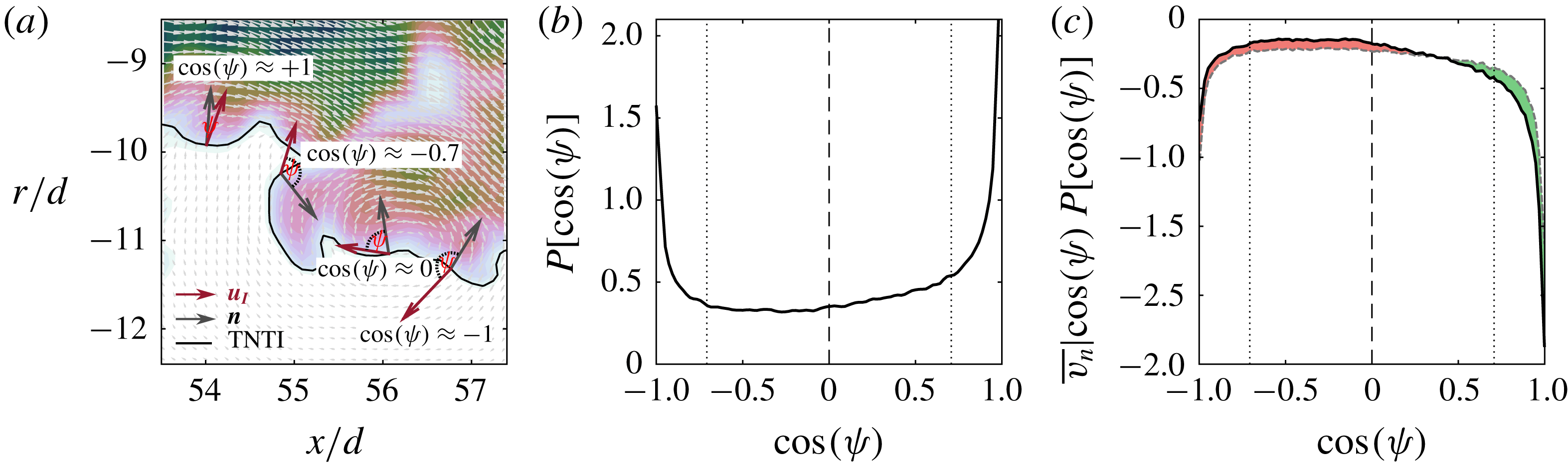
Figure 9(c) plots
 $\overline{v_{n}}$
conditioned on
 $\cos (\unicode[STIX]{x1D713})$
. The filled green area shows that the conditional entrainment velocity is enhanced when
 $\cos (\unicode[STIX]{x1D713})>0.5$
and maximised as
 $\cos (\unicode[STIX]{x1D713})\rightarrow 1$
, i.e. when local fluid vectors form an impinging flow pattern. At
 $\cos (\unicode[STIX]{x1D713})=1$
,
 $\overline{v_{n}}|_{cos(\unicode[STIX]{x1D713})=1}$
is 45 % greater than
 $\overline{v_{n}}$
. The filled red area shows that alignments of
 $\cos (\unicode[STIX]{x1D713})<0.5$
act to suppress local entrainment as the local flow field is either moving tangentially to the interface (
 $\cos (\unicode[STIX]{x1D713})\approx 0$
) or advecting normally towards the non-turbulent region (
 $\cos (\unicode[STIX]{x1D713})\rightarrow -1$
).
The observation that local advection of the TNTI towards the turbulent region corresponds with greater local entrainment rates along the interface is consistent with the TNTI geometry dependence of entrainment presented in figure 8. One can expect that a flow pattern that advects the TNTI towards the turbulent region (i.e.
 $\cos (\unicode[STIX]{x1D713})\approx 1$
) may be associated with large-scale motions that transport the TNTI nearer to the centreline of the jet (
 $r_{I}<\overline{r_{I}}$
) and also smaller-scale motions that produce convex curvatures (see figure 6). Both scenarios correspond with an increase in the local entrainment rate.
We now consider the relationship between the local fluid velocity magnitude and the local entrainment rate. For this we decompose
 $\boldsymbol{u}_{I}$
into the local normal velocity
 $u_{n}$
and the tangent velocity
 $u_{t}$
, as shown in figure 10. The normal and tangential velocity components are determined by the dot product of the local fluid velocity and the interface unit vectors,
 $$\begin{eqnarray}\displaystyle & \displaystyle u_{n}=\boldsymbol{u}\boldsymbol{\cdot }\boldsymbol{n}, & \displaystyle\end{eqnarray}$$
 $$\begin{eqnarray}\displaystyle & \displaystyle u_{t}=\boldsymbol{u}\boldsymbol{\cdot }\boldsymbol{t}. & \displaystyle\end{eqnarray}$$
 $u_{n}$
and
 $u_{t}$
along the TNTI are illustrated in figure 10(b) and exhibit approximate Gaussian behaviour as expected (Batchelor Reference Batchelor1953). This is in contrast to the non-Gaussian behaviour observed for the entrainment velocity in figure 4(c). The distributions
 $P(u_{n})$
and
 $P(u_{t})$
have positive mean values, which indicates that the mean flow is advecting the TNTI towards the turbulent region of the jet and generally along the positive streamwise direction.
(a) Schematic of the interface-normal velocity (
 $u_{n}$
, red arrows) and tangent velocity (
 $u_{t}$
, blue arrows) along the TNTI. The local interface-normal unit vector (
 $\boldsymbol{n}$
) is depicted with the grey arrows. (b) PDF of
 $u_{n}$
(red) and
 $u_{t}$
(blue) measured along the TNTI. A Gaussian distribution is shown by the dashed black line. (c) Conditionally mean entrainment velocity based on the interface-normal velocity
 $\overline{v_{n}}|_{u_{n}}P(u_{n})$
, solid line. The unconditioned mean entrainment velocity is denoted by the dashed line for
 $\overline{v_{n}}P(u_{n})$
. Green fill indicates the values of
 $u_{n,t}$
for which the conditional mean entrainment velocity is greater than the mean entrainment velocity; red fill indicates values for which there is a reduction in entrainment. (d) As for (c) but for the interface-tangent velocity
 $u_{t}$
.
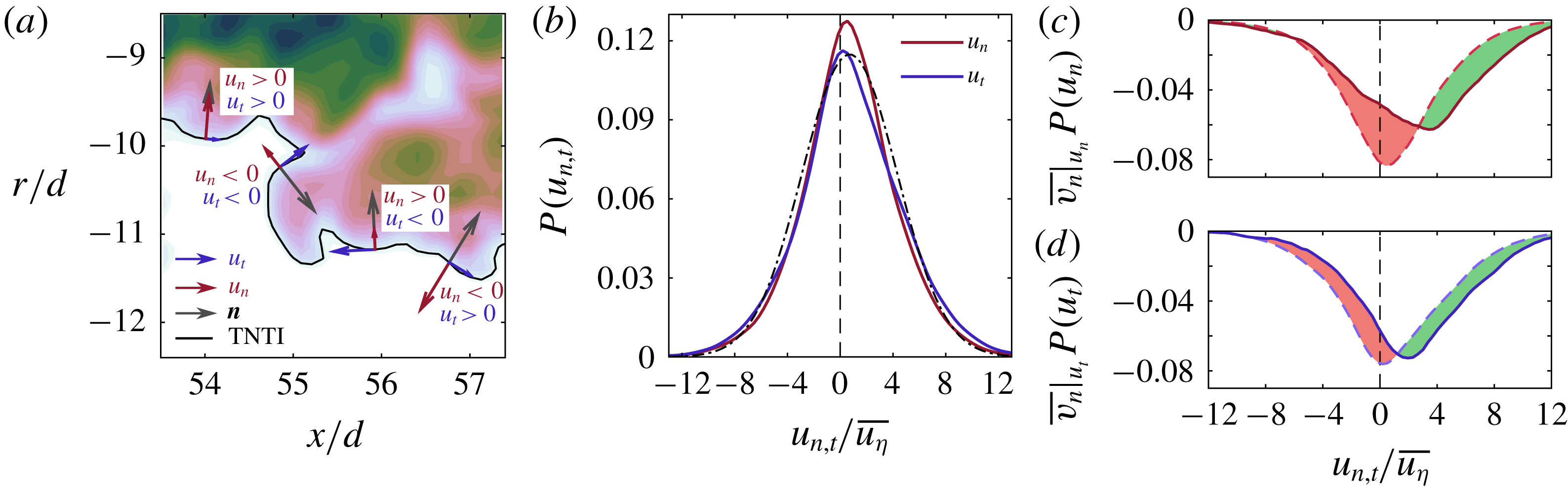
The relationship between the entrainment velocity and component velocities of
 $\boldsymbol{u}_{I}$
,
 $u_{n}$
and
 $u_{t}$
, are presented in figure 10(c,d). Generally, greater entrainment occurs when
 $u_{n}>3\overline{u_{\unicode[STIX]{x1D702}}}$
and
 $u_{t}>1\overline{u_{\unicode[STIX]{x1D702}}}$
(i.e. large and positive). The largest reduction in entrainment occurs when the local fluid momentum approaches zero (
 $u_{n}\approx 0$
and
 $u_{t}\approx 0$
). This emphasises the beneficial role local kinematics play in enhancing local entrainment because in the absence of momentum the entrainment rate is diffusion limited. The interface-normal velocity (figure 10
c) shows greater influence on the conditional mean entrainment velocity compared to the interface-tangent velocity (figure 10
d), which is similar to the conditional entrainment velocity behaviour observed in figure 9(c).
We may summarise the findings in this section as follows: the entrainment velocity has a characteristic length scale of the order of the Taylor micro-scale, which is comparable to the dominant length scale of velocity fluctuations along the TNTI. Whilst the radial position of the TNTI exhibits large-scale motions of the order of the jet half-width, the interface also exhibits very small contortions that are characterised by surface curvature. These geometric features of the TNTI influence the local entrainment velocity. Entrainment is enhanced when the TNTI is nearer to the jet centreline and in regions where the curvature is convex to the turbulent region. In addition, the local entrainment is either enhanced or suppressed depending on the alignment between the local flow and the interface normal. In particular, local entrainment is enhanced when the local fluid velocity is oriented normal to the TNTI and pointing towards the turbulent region (positive interface-normal fluid velocity,
 $u_{n}$
). Conditional averages presented in this section only consider the local geometric and flow features in the immediate vicinity of the TNTI. To gain further insight into the role of the flow kinematics on the local entrainment rate we must consider the flow fields adjacent to both sides of the TNTI; this is presented in the following section.
4 Conditional flow structures about the TNTI
4.1 Conditioning along coordinates normal to the TNTI
We now expand the analysis of the previous section and consider the local flow on either side of the TNTI to understand the kinematics associated with entrainment and detrainment rates. To do this we evaluate profiles along the interface-normal coordinate
 $x_{n}$
, as described in § 2.1. The
 $x_{n}$
-profiles presented in this section are also conditioned on the local entrainment velocity along the TNTI, which is divided into the two regimes illustrated in figure 4(c). Entrainment is defined as
 $v_{n}\leqslant 0$
and is represented by green square markers and detrainment is defined as
 $v_{n}>0$
and is represented by red triangle markers. The decomposition of the
 $x_{n}$
-profiles based on these two regimes offers insight into the features of the flow that either enhance or hinder entrainment.
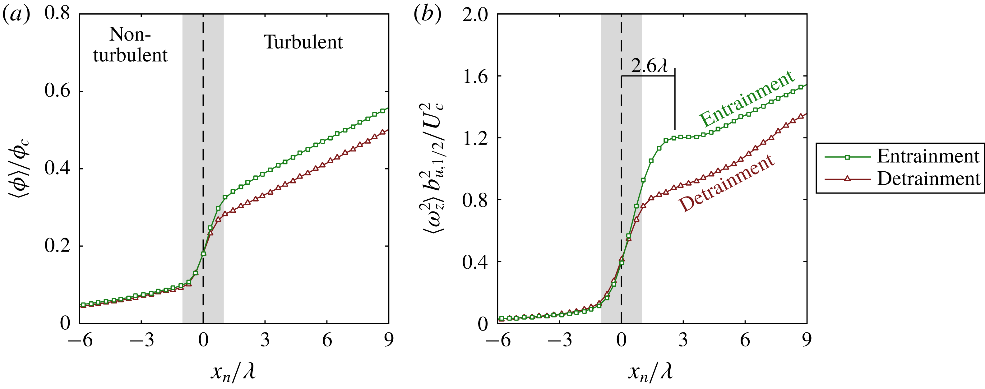
(a) Conditionally averaged profile of scalar concentration along
 $x_{n}$
. The turbulent region is defined as
 $x_{n}>0$
and the non-turbulent region is defined as
 $x_{n}<0$
. Entrainment is denoted by green squares and detrainment is denoted by red triangles. (b) As for (a) but with the enstrophy field
 $\unicode[STIX]{x1D714}_{z}^{2}$
.
(a) Graphical description of the flow quantities measured along the interface-normal coordinate,
 $x_{n}$
. Mean conditionally averaged profiles locally normal to the TNTI (black lines) for (b)
 $u_{n}$
and (c)
 $u_{t}$
. Further conditioning on the local entrainment velocity is shown by the coloured markers, as defined in figure 4(c). Positive entrainment is denoted by green squares and detrainment is denoted by red triangles. The turbulent region is defined as
 $x_{n}>0$
and the non-turbulent region is defined as
 $x_{n}<0$
. The entrainment-conditioned mean (d) interface-normal and the (e) interface-tangent velocities at the interface (
 $x_{n}=0$
).

Figure 11(a,b) shows the jump profiles for
 $\langle \unicode[STIX]{x1D719}\rangle$
and
 $\langle \unicode[STIX]{x1D714}_{z}^{2}\rangle$
across the TNTI (as shown in § 2.1) but with additional conditioning on the local entrainment velocity (coloured markers). Inside the turbulent region (
 $x_{n}>0$
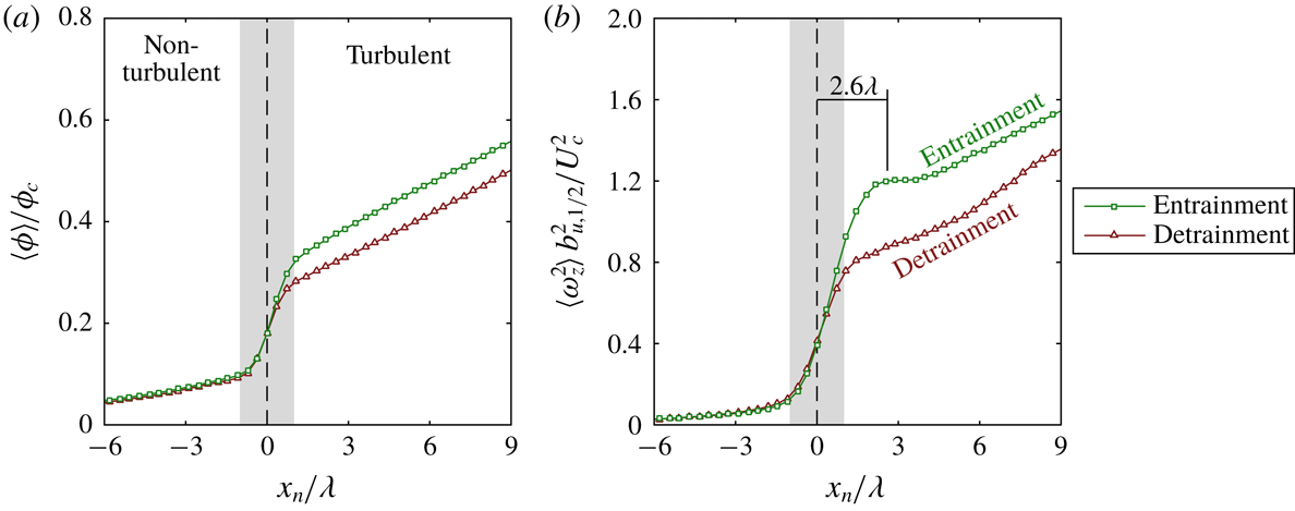
) the scalar concentration and vorticity magnitudes are greater during entrainment (green squares) compared to detrainment (red triangles). Notably, the jump in enstrophy that accompanies entrainment extends
 $x_{n}=2.6\unicode[STIX]{x1D706}$
into the turbulent region and is approximately
 $45\,\%$
larger than the enstrophy magnitude during detrainment. This increase in enstrophy that accompanies entrainment may be explained by previous observations of Taylor micro-scale vortical structures of
 $O(\unicode[STIX]{x1D706})$
in size that populate the inner edges of the TNTI (da Silva & Taveira Reference da Silva and Taveira2010). We conjecture that these high intensity vortex structures along the TNTI are correlated with the local entrainment process across the interface.
4.2 Conditional flow field about the TNTI
We now consider the flow field about the TNTI by decomposing the fluid velocity (
 $\boldsymbol{u}$
) along
 $x_{n}$
into the normal
 $u_{n}$
and tangential
 $u_{t}$
components relative to the TNTI. Figure 12(a) illustrates the component velocities along the coordinate
 $x_{n}$
. Both
 $u_{n}$
and
 $u_{t}$
are calculated at each point along
 $x_{n}$
(see (3.3)), normalised by
 $U_{c}$
and ensemble averaged across the TNTI and over all the realisations of the flow. The mean profiles of
 $\langle u_{n}\rangle$
and
 $\langle u_{t}\rangle$
correspond to the thick black lines presented in figures 12(b) and 12(c), respectively. The profiles denoted by the coloured markers will be discussed later. The filled grey region in the background spans
 $x_{n}=\pm \unicode[STIX]{x1D706}$
and represents the region over which the jump in
 $\langle \unicode[STIX]{x1D719}\rangle$
and
 $\langle \unicode[STIX]{x1D714}_{z}^{2}\rangle$
occurs (see figure 11).
Figure 12(b,c) shows the profiles of
 $\langle u_{n}\rangle -\langle u_{n}(0)\rangle$
and
 $\langle u_{t}\rangle -\langle u_{t}(0)\rangle$
, normalised by
 $U_{c}$
, along
 $x_{n}$
. Component velocities along
 $x_{n}$
are subtracted by a reference component velocity of
 $\boldsymbol{u}_{I}$
at the TNTI (
 $x_{n}=0$
) resulting in a transformation that depicts the flow field in a frame of reference moving with the local fluid velocity
 $\boldsymbol{u}_{I}$
at the TNTI. The profile of
 $\langle u_{n}\rangle -\langle u_{n}(0)\rangle$
in figure 12(b) shows (in black solid line) that relative to the TNTI
 $u_{n}$
is positive in the non-turbulent region and transports irrotational fluid towards the TNTI. In the turbulent region, relative to the TNTI fluid velocity,
 $u_{n}$
is negative corresponding to the transport of rotational fluid towards the TNTI. Similar profiles have been observed across a number of numerical an experimental studies in wakes and jets (Bisset et al.
Reference Bisset, Hunt and Rogers2002; Westerweel et al.
Reference Westerweel, Fukushima, Pedersen and Hunt2009; Watanabe et al.
Reference Watanabe, Sakai, Nagata, Ito and Hayase2014a
; da Silva, Taveira & Borrell Reference da Silva, Taveira and Borrell2014b
), however, the physical relationship between these conditionally averaged counterflow profiles, the entrainment velocity and the local kinematics about the TNTI have not been investigated. The tangential velocity profile (black line) in figure 12(c) shows the flow is reasonably quiescent in non-turbulent region and increases with
 $x_{n}$
into the turbulent region of the jet. This behaviour is qualitatively similar to observations by Westerweel et al. (Reference Westerweel, Fukushima, Pedersen and Hunt2009) (see their figure 13).
Similar to the analysis performed in figure 11, we decompose the interface-normal
 $\langle u_{n}\rangle$
and interface-tangent
 $\langle u_{t}\rangle$
velocity profiles based on the local entrainment velocity
 $v_{n}$
measured at the TNTI (
 $x_{n}=0$
). The velocity profiles in figure 12(b,c) are further conditioned on entrainment and detrainment as illustrated in figure 4(c), as denoted by the coloured lines and markers. Conditioning the interface-normal velocity profile on
 $v_{n}$
, as shown in figure 12(b), reveals substantial differences in the profiles. The entrainment and detrainment profiles rapidly diverge in the turbulent region (
 $x_{n}>0$
). Entrainment (green squares) shows a significant increase in
 $-\langle u_{n}\rangle$
in the turbulent region, which significantly enhances the transport of turbulent fluid towards the TNTI compared to the mean profile (black line). Therefore high levels of entrainment at the interface are accompanied by the greater transport of momentum, scalar and vorticity from the turbulent region towards the TNTI of the jet. This is in contrast to the detrainment profile (red triangles), which shows that
 $\langle u_{n}\rangle$
becomes positive in the turbulent region, after
 $x_{n}/\unicode[STIX]{x1D706}=5$
, as it transports fluid away from the TNTI. This is consistent with the shedding of turbulent fluid into the non-turbulent region. In addition to not exhibiting a counterflow profile about the TNTI that extends very far into the turbulent region, several other differences between the entrainment and detrainment profiles are observed. The velocity difference across the TNTI is noticeably larger for the entrainment profile and the interface-normal velocity gradient is also steeper, and extends through the turbulent region, for entrainment. This suggests that the velocity gradient in the vicinity of the TNTI may play an important role in determining the local kinematics of entrainment/detrainment across the TNTI. The characteristic flow patterns for positive entrainment and detrainment are shown in figure 12(b) and support the observations from the previous sections that show that entrainment and detrainment strongly depend on the alignment of the local velocity and the TNTI normal
 $\boldsymbol{n}$
.
The component values of
 $\boldsymbol{u}_{I}$
, the interface-normal
 $\langle u_{n}(0)\rangle$
and interface-tangent
 $\langle u_{t}(0)\rangle$
at the TNTI are plotted in figures 12(d) and 12(e), respectively. Figure 12(d) shows that there is greater inflow of non-turbulent fluid (
 $u_{n}>0$
) towards the turbulent region during entrainment compared to detrainment. The positive values signify that the fluid velocity is aligned with the interface-normal
 $\boldsymbol{n}$
in the direction of the turbulent region. The interface-tangent velocity
 $\langle u_{t}(0)\rangle$
is also larger during positive entrainment compared to detrainment. The entrainment-conditioned profiles in figure 12(c) are qualitatively similar, which suggests that the tangential shear across the TNTI is not very different during entrainment and detrainment.
Based on the conditional profiles in figures 11 and 12 we may summarise some key physical features that influence the local entrainment process as follows: (i) the larger jump in enstrophy that is correlated with entrainment compared with detrainment (figure 11 b) points to the role of intense Taylor micro-scale vortical structures in the vicinity of the TNTI (to be discussed in the next section) previously observed by da Silva & Taveira (Reference da Silva and Taveira2010), (ii) the transport of turbulent fluid towards the TNTI is enhanced during entrainment whereas turbulent fluid is advected away from the TNTI during detrainment (figure 12 b) and (iii) transport of non-turbulent fluid towards the TNTI is enhanced during entrainment compared with detrainment (figure 12 d). Features (ii) and (iii) show that increased local entrainment is associated with a distinct counterflow velocity profile about the TNTI that extends well into the turbulent region. Thus, we may now address part of the second research question posed in the introduction: is there a characteristic turbulent structure that influences the local entrainment along the TNTI?
4.3 Instantaneous entrainment
Here, we build upon previous observations that along and adjacent to the TNTI the turbulent region is populated by intense vortical structures of
 $O(\unicode[STIX]{x1D706})$
(da Silva & Taveira Reference da Silva and Taveira2010). These structures potentially offer an explanation for (i) the jump in enstrophy observed in figure 11(b) and (ii) the generation of the characteristic counterflow profile about the TNTI, both of which are correlated with increased local entrainment. Furthermore, the correlation
 $R_{v_{n}^{\prime }v_{n}^{\prime }}$
in figure 5(a) showed us that fluctuations of the entrainment velocity along the TNTI occur with spacing between them that is
 $O(\unicode[STIX]{x1D706})$
.
In figures 13 and 14 we present instantaneous snapshots of the flow in the region about the TNTI that depict these intense
 $\unicode[STIX]{x1D706}$
-scale vortical structures and the scalar fields in different reference frames to elucidate the local kinematic features of entrainment. These snapshots are extracted from the high-resolution SFOV data for which the vector spacing is
 $3\unicode[STIX]{x1D702}$
. In the first column we show instantaneous scalar concentration fields normalised by the local mean centreline concentration,
 $\unicode[STIX]{x1D719}/\unicode[STIX]{x1D719}_{c}$
, with the velocity vectors overlaid in grey in a laboratory reference frame. The TNTI is indicated by the black line and the entrainment velocity denoted by the green vectors for positive entrainment (
 $v_{n}\leqslant 0$
) and red vectors for detrainment (
 $v_{n}>0$
). In the second column the velocity field is plotted in a reference frame moving with the TNTI local fluid velocity at a point denoted by the red circle (
 $\boldsymbol{u}_{I}$
). In the third column, also in the TNTI fluid reference frame (flow velocity vectors in the middle column), the
 $\unicode[STIX]{x1D719}$
-field is replaced with the spanwise vorticity field,
 $\unicode[STIX]{x1D714}_{z}$
.
(a,d,g) Instantaneous scalar concentration field (background contours) superimposed with the TNTI (black line), local fluid vectors in a laboratory reference frame (grey vectors) and the entrainment velocity vectors along the TNTI. The entrainment velocity vectors are colour coded as per figure 4(c): green vectors denote entrainment and red vectors denote detrainment. (b,e,h) Same data as (a,d,g) but with the fluid vectors shown in a frame of reference moving with the TNTI fluid velocity at the point denoted by the red circle. (c,f,i) Same data as (b,e,h) but with the vorticity field shown in the background contours.

See caption in figure 13.

Figure 13 shows three examples of high entrainment rates. It is difficult to discern a characteristic flow pattern associated with entrainment in a laboratory reference frame, figure 13(a,d,g). By considering a frame of reference moving with the interface fluid in the second column (b,e,h), we observe a counterflow about the TNTI in which both turbulent and non-turbulent fluids converge onto the TNTI. This is consistent with the counterflow
 $u_{n}$
profiles conditioned for entrainment (green squares) shown in figure 12(b). Furthermore, these counterflow fields also coincide with vortex structures on the turbulent side of the TNTI, as shown in figure 13(c,f,i), which are located in the vicinity of the entrainment (i.e. negative
 $v_{n}$
). It is reasonable to conjecture that these vortex structures, which are
 $O(\unicode[STIX]{x1D706})$
, result in the enstrophy jump observed in the conditionally averaged
 $x_{n}$
profiles of
 $\langle \unicode[STIX]{x1D714}_{z}^{2}\rangle$
in figure 11(b).
The conditional statistics and instantaneous flow fields are evidence that these Taylor micro-scale vortex structures along the TNTI play an important role in the local entrainment process. The diameter of the vortices, which are
 $O(\unicode[STIX]{x1D706})$
, are illustrated in figure 13(c,f,i) and, to be later discussed, in figure 14(c,f,i). Although, we focus on the role of these vortex structures in the kinematics of entrainment, previous studies have shown that the thickness of the TNTI scales with their size (da Silva & Taveira Reference da Silva and Taveira2010). In addition, Taveira, da Silva & Pereira (Reference Taveira, da Silva and Pereira2011) demonstrate that these vortex cores generate a local pressure minimum and a peak in the pressure variance located
 $x_{n}=2\unicode[STIX]{x1D706}-4\unicode[STIX]{x1D706}$
into the turbulent region from the TNTI, which agrees very well with the local enstrophy peak that we measure in figure 11(b) that occurs at
 $x_{n}=2.6\unicode[STIX]{x1D706}$
, and in accordance with the
 $R_{v_{n}^{\prime }v_{n}^{\prime }}$
results in figure 5(a).
Combining these observations suggests that the pressure gradient field generated by these vortex structures acts to induce greater inflow of non-turbulent fluid towards the TNTI and generates a counterflow velocity field. The conditional profiles shown in figures 11(b) and 12(c) demonstrate that this particular kinematic description is associated with a local increase in entrainment. The work of Watanabe et al. (Reference Watanabe, Sakai, Nagata, Ito and Hayase2014b
) offers an explanation as to why a counterflow velocity profile is associated with greater entrainment. Watanabe et al. (Reference Watanabe, Sakai, Nagata, Ito and Hayase2014b
) found that the flow conditions about the TNTI that would yield alignment of the compressive strain eigenvector (
 $\unicode[STIX]{x1D6FE}$
) with the interface-normal unit vector (
 $\boldsymbol{n}$
), would also yield alignment of the extensive strain eigenvector (
 $\unicode[STIX]{x1D6FC}$
) parallel to the TNTI and also parallel to the vorticity vector (
 $\unicode[STIX]{x1D74E}$
, Gampert et al.
Reference Gampert, Boschung, Hennig, Gauding and Peters2014). Alignment of the extensive strain with the vorticity vector occurs in region of positive enstrophy production (Buxton & Ganapathisubramani Reference Buxton and Ganapathisubramani2010). Equation (1.1), supported by van Reeuwijk & Holzner (Reference van Reeuwijk and Holzner2014) and Philip et al. (Reference Philip, Bermejo-Moreno, Chung and Marusic2015), tells us that viscous dissipation is the primary source of detrainment. Thus, a strain field that intensifies the vorticity of the
 $\unicode[STIX]{x1D706}$
-scale structures along the TNTI will counter the effects of viscous dissipation and promote greater local entrainment.
Following from the arguments above, it is reasonable to expect that misalignment of
 $\unicode[STIX]{x1D6FE}$
with
 $\boldsymbol{n}$
, or simply a weaker compressive strain rate, would correspond with the destruction of enstrophy. In the absence of enstrophy production, a vortex will decay via viscous dissipation which results in detrainment. In other words, a fluid particle that once contained vorticity greater than the threshold defining the TNTI, will dissipate vorticity, which then falls below the TNTI threshold and therefore crosses from the turbulent region to the non-turbulent region. Thus
 $\unicode[STIX]{x1D706}$
-scale vortices along the TNTI are conjectured to play a key role in local entrainment and detrainment processes in turbulent shear flows, in support of past research on the TNTI (Westerweel et al.
Reference Westerweel, Fukushima, Pedersen and Hunt2005, Reference Westerweel, Fukushima, Pedersen and Hunt2009; da Silva & Taveira Reference da Silva and Taveira2010; Chauhan et al.
Reference Chauhan, Philip, de Silva, Hutchins and Marusic2014b
). In the next section, we present a series of instantaneous fields to illustrate this conjecture by considering how the entrainment kinematics can be observationally linked to the presence of adjacent vortical structures.
4.4 Instantaneous detrainment
Figure 14 illustrates three instantaneous flow snapshots of detrainment along the TNTI. In figure 14(c) we see the TNTI forms a perimeter around a vortex-pair structure. In the region about the origin of
 $x_{n}$
(red circle) in (b) the local flow is impinging onto the TNTI resulting in positive entrainment. To the left of the panels in (a,b,c) red vectors indicating detrainment occur due to the flow moving tangential to the TNTI. Again, in figure 14(e,f), we observe a local flow field where flow is advected across the TNTI resulting in detrainment. Entrainment are also observed in regions where a counterflow field is established. Finally, figure 14(g,h,i) depicts large detrainment which occupies most of the FOV. It is difficult to discern any notable flow pattern based on the laboratory reference frame flow field (grey vectors) in panel (g). However, from a frame of reference moving with the TNTI fluid at the point denoted by the red circle we observe a sweeping flow pattern on the right side of panels (h,i) in which the fluid is moving in the same direction on either side of the TNTI. This advection flow pattern results in a large detrainment rate and distinctly contrasts the clear impinging flow pattern observed in the previous entrainment cases.
Distribution of the local entrainment velocity
 $v_{n}$
as a function of spatial filter size
 $\unicode[STIX]{x1D6E5}$
. With larger filter sizes there is a reduction in detrainment (
 $v_{n}>0$
) whilst the entrainment remains relatively unchanged.

Thus, the interface-normal velocity profiles presented in figure 12(b) are evidenced in instantaneous flow patterns about the TNTI. We have shown in this section that (i) the vortical structures adjacent to the TNTI exhibit greater enstrophy during entrainment compared to detrainment, (ii) there is large-scale advection of turbulent fluid towards the TNTI during entrainment and (iii) there is greater inflow of non-turbulent fluid towards the TNTI during entrainment. These flow features are manifested as a counterflow velocity profile about the TNTI in a frame of reference moving with the TNTI fluid particle. We postulate that the strain fields that correspond with these flow patterns, and the resultant balance between enstrophy production and dissipation, is strongly coupled with the resultant local entrainment at the interface.
4.5 Remarks on the fluctuating nature of the entrainment velocity and size of entrainment/detrainment structures
It is clear from the two point correlation of the fluctuating
 $v_{n}$
along the TNTI (
 $R_{v_{n}^{\prime }v_{n}^{\prime }}$
) in figure 5(a) that the local entrainment undergoes a periodic fluctuation with a wavelength that is of
 $O(\unicode[STIX]{x1D706})$
. The physical reason for these fluctuations is the numerous
 $\unicode[STIX]{x1D706}$
-sized eddies located around along the TNTI. These eddies are observed vividly in the last columns of figures 13 and 14. To be specific, if we pick figure 14(c), we see that along the TNTI a
 $\unicode[STIX]{x1D706}$
-sized eddy promotes entrainment (green arrows) on one side and at the same time gives rise to detrainment (red arrows). The fluid particles are drawn into the turbulent region on one side and almost in tandem there is a tendency of the fluid particles to be pushed out of the turbulent region. This action of eddies at the TNTI may be the main reason for the varying entrainment and detrainment rates that occur along the TNTI.
Even though entrainment and detrainment rates are driven by eddies at the TNTI, these are heavily dependent on the local TNTI surface features (as detailed in § 3.3). In fact, there is also a length-scale dependence of entrainment and detrainment rates. Evidence of this length-scale dependence may be obtained by filtering the original velocity/scalar fields, as explained in detail in Mistry et al. (Reference Mistry, Philip, Dawson and Marusic2016). In short, the fields are box filtered with different filter sizes (
 $\unicode[STIX]{x1D6E5}$
), and entrainment velocities are recalculated using the same procedure as for the unfiltered case. The PDF of
 $v_{n}$
for different filter widths (normalised by
 $\unicode[STIX]{x1D706}$
) is shown in figure 15. With increasing filter width the smaller features are eliminated from the flow, and as evidenced in figure 15, the detrainment velocities are the most affected by the filtering. In fact, the large detrainment rates are ones to be eliminated in the filtering procedure, which implies that they are associated with smaller scales. The fact that entrainment is largely unaffected by this filtering process suggests a large-scale influence on entrainment, likely resulting from the global constraints of a constant mean axial momentum flux and energy dissipation (cf. § 1).
5 Summary and conclusions
In this paper we investigate the kinematics of local entrainment with respect to the turbulent/non-turbulent interface in the far field of an axisymmetric jet at high Reynolds number. We performed high-speed, simultaneous multi-scale PIV and PLIF measurements that allowed for the identification of the TNTI using a passive scalar and measurement of the local entrainment velocity along it. In agreement with other studies of the entrainment velocity (Holzner & Lüthi Reference Holzner and Lüthi2011; Wolf et al.
Reference Wolf, Lüthi, Holzner, Krug, Kinzelbach and Tsinober2012; Watanabe et al.
Reference Watanabe, Sakai, Nagata, Ito and Hayase2014a
; Krug et al.
Reference Krug, Holzner, Lüthi, Wolf, Kinzelbach and Tsinober2015), we show that the PDF of
 $v_{n}$
is non-Gaussian and that
 $v_{n}$
is intermittent along the TNTI. We observe that the net entrainment of non-turbulent fluid into the turbulent region is balanced by approximately two parts of entraining flow and one part of detraining flow. The integral length scale of the entrainment velocity is of
 $O(\unicode[STIX]{x1D706})$
, which supports the role of Taylor micro-scale eddies in the entrainment/detrainment process.
We characterise three features of the TNTI geometry: the radial position, the interface curvature and the surface orientation, the PDFs of which all agree well with comparable studies (Dopazo et al.
Reference Dopazo, Martin and Hierro2007; Wolf et al.
Reference Wolf, Lüthi, Holzner, Krug, Kinzelbach and Tsinober2013b
; Watanabe et al.
Reference Watanabe, Sakai, Nagata, Ito and Hayase2014a
). To understand the effect of these TNTI geometric properties on entrainment velocity, we also evaluate the conditional entrainment velocity as a function of these three variables. Generally, there is greater local entrainment along the TNTI while the interface radial position is nearer to the jet centreline, while the surface curvature is convex and along the leading edges of the interface. On the other hand, detrainment is more likely to happen when the radial location is away from the jet centreline, the TNTI surface is concave and the location is along the jet’s trailing edge. This is summarised in figure 16(a). Furthermore, there is greater entrainment when the local fluid velocity vector
 $\boldsymbol{u}_{I}$
is aligned with the local interface-normal unit vector
 $\boldsymbol{n}$
. This entrainment dependence on velocity, specifically the interface-normal velocity, goes towards explaining why there is a higher entrainment near the jet centreline and along convex curvatures.
Summary of the entrainment and detrainment relative to the TNTI geometric features. We recall that negative
 $v_{n}$
(pointing away from the TNTI) implies entrainment and an opposite sign for detrainment: (a)
 $v_{n}$
in the laboratory reference frame; (b) fluid velocity conditioned on the interface (
 $\langle u_{n}\rangle$
) relative to the TNTI location,
 $\langle u_{n}\rangle -\langle u_{n}(0)\rangle$
.
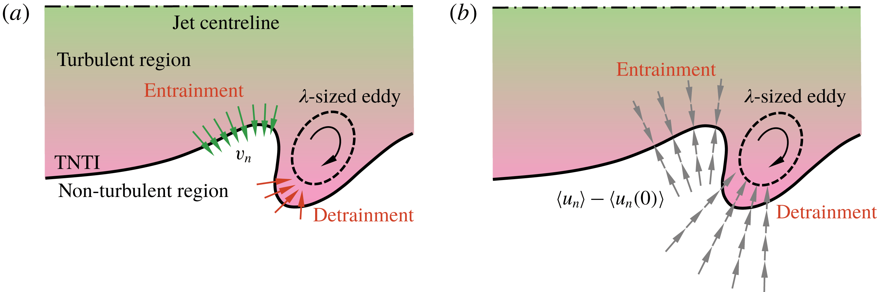
Using velocity profiles in an interface reference frame along an interface-normal coordinate
 $x_{n}$
, we determine that the velocity tangential to the TNTI does not significantly influence the local entrainment velocity. Rather, it is the interface-normal velocity that correlates well with the local entrainment. Entrainment rates correspond with a counterflow velocity profile that results in both turbulent fluid and non-turbulent fluid being simultaneously transported towards TNTI. We present evidence using instantaneous snapshots and mean profiles of enstrophy about the TNTI to demonstrate that intense
 $\unicode[STIX]{x1D706}$
-scale structures along the TNTI are responsible for the generation of a compressive strain field normal to the TNTI, which is manifested as the counterflow velocity profile that we observe. We interpret the flow kinematics by considering the local strain field and the resultant enstrophy amplification or destruction. A strong counterflow, and compressive strain, is likely to be associated with a similarly large extensive strain eigenvector that will intensify the vorticity at a rate that is faster than viscous dissipation of enstrophy. In the absence of enstrophy production, the dissipation dominates leading to the conversion of turbulent fluid to non-turbulent one, and hence local detrainment. This picture of the local entrainment/detrainment process is illustrated in the schematic in figure 16(b). Furthermore, the instantaneous flow fields clearly show the role of
 $O(\unicode[STIX]{x1D706})$
-eddies in varying the entrainment along the TNTI. In fact, it is not uncommon to see the entrainment and detrainment accompanied by each other along the TNTI wrapped around the
 $O(\unicode[STIX]{x1D706})$
-eddies. This also provides some kinematic explanation of the large entrainment and detrainment rates on a jet TNTI.
Acknowledgements
The authors wish to thank the UK Engineering and Physical Sciences Research Council (research grant no. EP/I005897/1), the Norwegian Research Council (research grant no. 244386) and the Australian Research Council for the financial support of this work. The visit of D.M. to the University of Melbourne was supported by the David Crighton Fellowship from the Department of Applied Mathematics and Theoretical Physics, Cambridge.