Introduction

Antarctica is one of the most important factors in the global climate system. It contains 90% of the world’s ice; melting all the Antarctic ice would produce a 65 m rise in sea level (Oerlemans, 1993). A loss of only 1% of the Antarctic ice volume would significantly affect sea level and hence human life. The annual snowfall on the grounded Antarctic ice is equivalent to about 5 mm a^–1 of global sea-level change (Jacobs, 1992), so yearly variations of snowfall on the Antarctic can measurably affect sea level. Many glaciologists believe that the West Antarctic marine ice sheet is potentially unstable (Weertman, 1974; Hughes, 1975; Thomas and others, 1979). There are also sections of the East Antarctic ice sheet with beds well below sea level that might be unstable (Bentley and Sheehan, 1992).

Changes in the mass of the ice sheet would result in changes in its surface elevation. A major imbalance would produce elevation changes of as much as 1 ma^–1. However, small rates of change (a few centimeters per year) could arise from other causes; in particular, isostatic or tectonic changes in the height of the ice-sheet bed and interannual variations in the snow accumulation rate. Furthermore, it is not likely that snow accumulates at a constant rate through the year; an annual cycle in precipitation would appear as an annual cycle in surface height if the amplitude of the cycle were large enough.

Radar Altimetry

Satellite-borne radar altimetry is the only practical tool available at present for measuring the Antarctic surface elevation, considering the huge area that must be covered. (A laser altimeter in a high polar orbit is slated for launch early next century.) The satellite radar altimeter is designed to measure the travel time of a pulse of electromagnetic radiation that is transmitted downward to the Earth’s surface and scattered back to the satellite. The range between the satellite and the Earth’s surface beneath it is found by converting the two-way travel time to distance. The surface elevation referenced to an ellipsoid can be derived from the range measurement and the independently determined satellite orbit.

Geosat was launched in March 1985. Its primary mission was to provide a database for determining a marine geoid with a spatial resolution of 15 km. A second mission was begun 18 months after the primary mission. For the second mission the satellite was maneuvered into a 17 d repeat orbit (Born and others, 1987). This orbit, modeled after the 17 d repeat orbit for Seasat, was designed to monitor fluctuations of the sea surface. The ground track repeated to within ± 1 km every 17 d. An exact repeat orbit allows for the direct computation of sea-level variability by examining an ensemble of repeating ground tracks; it also provides an excellent opportunity for observing the temporal variation of the polar ice sheets. The Geosat Exact Repeat Mission (ERM) lasted 35 months, from November 1986 to September 1989. Our purpose in this paper is to examine the evidence for changing heights on a section of the surface of East Antarctica over a period of 32 months, using data from Geosat ERM. With essentially continuous observations, we were able to search for both cyclic and secular changes.

Waveform Retracking

The precision of satellite radar altimetry is not ideal for ice-sheet mass-balance studies, because the altimeter was designed for ocean studies. The height of a polar ice sheet varies laterally much more rapidly than that of the ocean surface. Altimeter data over the polar ice sheets need to be post-processed to produce accurate surface elevation measurements. The range-to-the-surface detector on board the satellite cannot react quickly enough to adjust to the rapid lateral changes in the height of an ice sheet; as a result the measured range can be substantially in error. Fortunately, return echoes from the surface (“waveforms”) are preserved for later analysis. Based upon the Brown surface-scattering model (Brown, 1977), Martin and others (1983) developed an algorithm for post-processing altimeter return waveforms from continental ice sheets. This algorithm was adopted by Zwally and others (1990) at NASA’s Goddard Space Flight Center to “retrack” all Seasat and Geosat waveforms over Greenland and Antarctica.

Ridley and Partington (1988) showed that volume scattering as well as surface scattering affects the waveform over Antarctica, and that neglecting volume scattering can introduce an error in elevation as large as 3 m, depending on the retracking method and location. Davis and Moore (1993) introduced a retracking algorithm that includes a volume-scattering term. The model they used yields an algorithm that fitted the waveform better than the NASA retracking algorithm (Davis and Moore, 1993), but it does not include the curvature of the Earth or the effect of an offnadir pointing angle. Yi and Bentley (1994) first introduced an algorithm that includes the curvature of the Earth and the pointing angle in the surface-scattering model but not in the volume-scattering model, and later added those factors to the volume-scattering models (Yi and Bentley, in press). Their algorithm can yield surface elevation values for individual waveforms. At the same time, quantitative estimates of the surface roughness, the proportion of volume scattering and penetration, and the regional and seasonal variations in those parameters can be obtained. In this study, the Geosat ERM waveform data were retracked using the model developed by Yi and Bentley (in press).

The received surface-scattered power is given by

This is a Brown model (Brown, 1977) modified to include the Earth’s curvature (Rodriguez, 1988). α and β are coefficients related to the speed of light, satellite height, antenna beam width and off-nadir pointing-angle effect; A’ will be eliminated during a normalization process, σ _c is related to surface roughness, and δ ≡ t – 2h/c (Yi and Bentley, 1994).

Fig. 1.

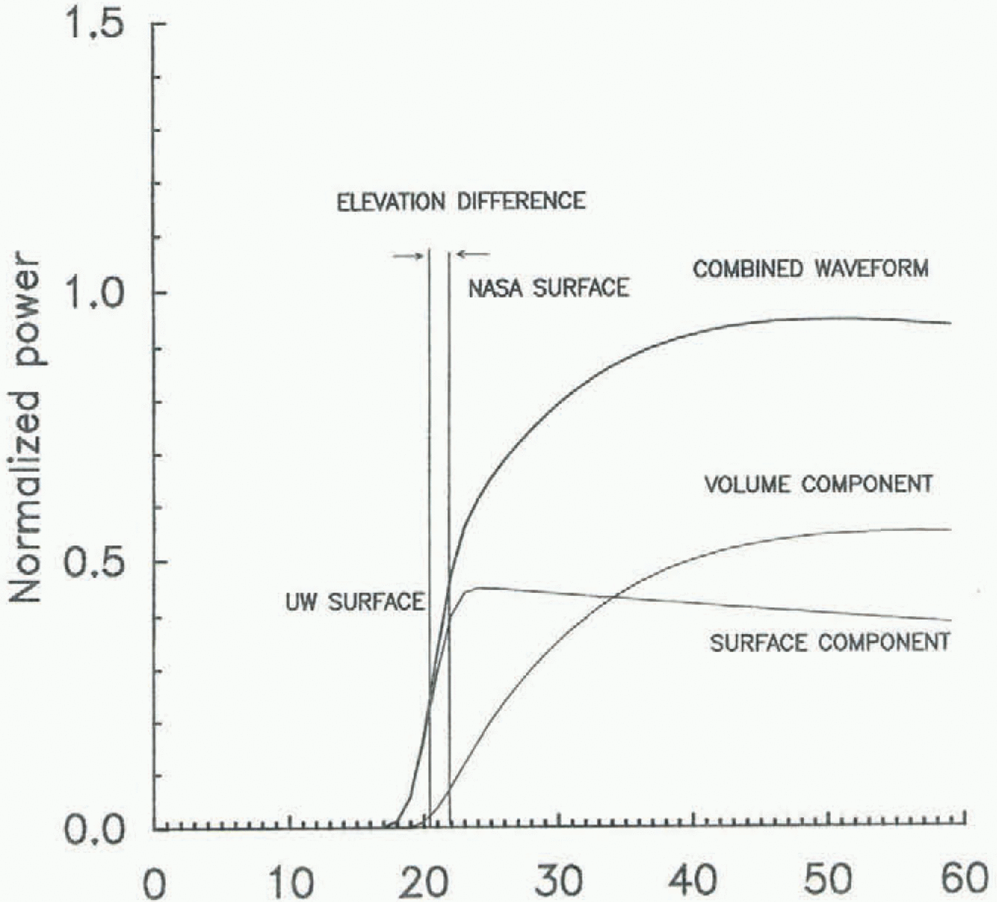
An idealized radar-altimeter echo, showing the contributions of the surface and volume components. The mean surface from our algorithm is defined by the mid-power point of the surface component (“UW surface”), whereas the NASA retracking method defines the mean surface by the mid-power point of the combined waveform (“NASA surface”). The distance corresponding to the difference between the two is the “elevation difference”. Each gate corresponds to a time interval of 3.125 ns, thus to a surface height difference of 0.47 m.

The received volume-scattered power from the depth range 0 – L is given by

where A is a constant related to snow surface and volume features, and k _e is the extinction coefficient (Yi and Bentley, in press).

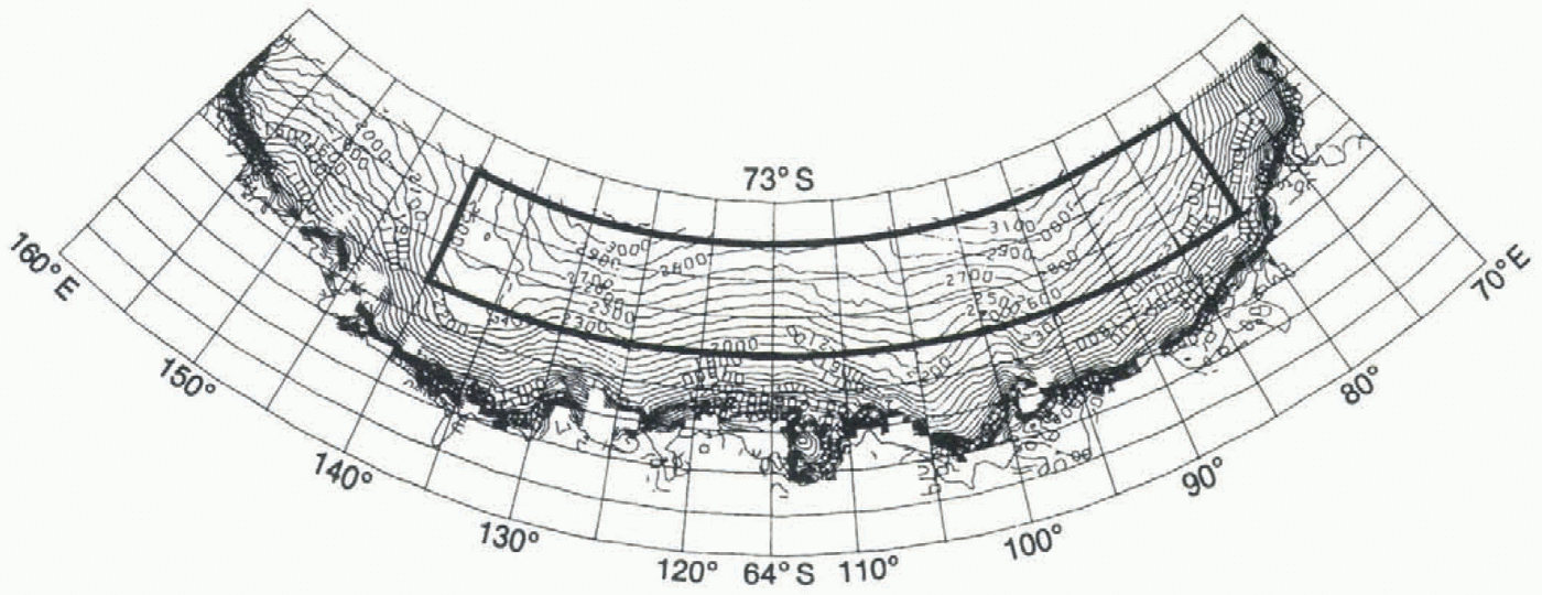
The surface-scattering and volume-scattering models were combined to fit the recorded altimeter waveforms using a non-linear least-square method. Figure 1 shows an example of a return-pulse shape according to the combined model. The model has been applied to the section of East Antarctica bounded by 80° E, 140° E, 69” S and 72.1° S. The highest 3° band of latitudes was chosen (Geosat coverage extended to 72.1 ° S) because the highest latitudes contains the densest measurements and because the surface in that band is smoother than at lower latitudes, so the waveforms are better behaved. A surface elevation map taken from Zwally and others (1983) is shown in Figure 2. Our study region is surrounded by a heavy-lined box.

Crossover Method

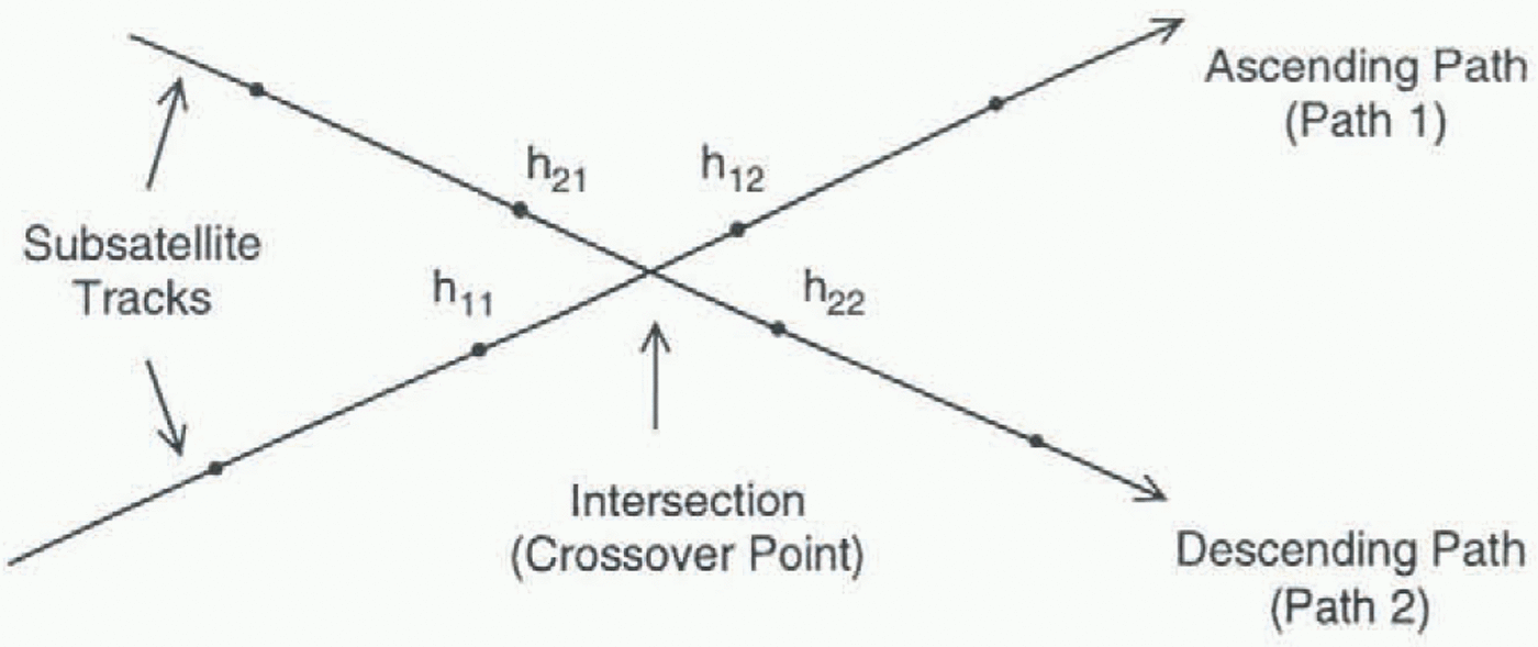
A standard crossover technique (Zwally and others, 1989; Lingle and others, 1990; Partington and others, 1991) was applied to the altimetry data for elevation-difference studies. A crossover point is a location where an ascending path (satellite traveling northward) intersects a descending path. Normally the crossover point of the two paths is not exactly at a measurement point. Figure 3 shows an example of calculating a crossover difference. If h ₁ and h ₂ are the true surface elevations at the crossover point at times t ₁ and t ₂, respectively, the measured elevation difference δh can be expressed

Fig. 2.

Map of the part of East Antarctica that includes our study area (69–72.1∘S, 80–140∘ E). The map with surface elevation contours is from Zwally and others (1983).

as δh = h ₂ – h ₁ + E, where E is a random error that includes orbit error, altimeter range measurement error and error introduced by interpolation. Normally E is larger than actual elevation changes. In order to acquire good estimates of surface elevation change, therefore, many crossover points need to be averaged to reduce E. The interpolation was carried out by assuming that the surface slopes linearly between tile two consecutive points. The absolute accuracy of the altimeter-derived elevations would increase if slope corrections were applied (since the return comes from the nearest point to the altimeter, not the point directly below it; Brenner and others, 1983), but, because we seek elevation change rather than absolute elevation, the slope correction was neglected. In the crossover procedure, we inherently assume that the pulse-limited footprint is located at the same place on the surface during successive transits, as usually is true (Zwally and others, 1989). The orbits for Geosat ERM were computed by Haines and others (1990) using the Goddard Earth Model (GEM) T2 gravitational potential field (Marsh and others, 1989). The GEM-T2 model was used rather than the newer JGM-2 model because the orbit adjustments by the latter model are not available for the last year of the ERM. The radial accuracies of the GEM-T2 orbit are estimated to be about 0.35 m rms (Haines and others, 1990).

Results

Thirty-five months of Geosat ERM data between latitudes 69∘ and 72.1∘ S and longitudes 80r∘ and 140∘ E were used in this study. Surface elevations for each month after the first

Fig. 3.

Crossover point geometry. h₁ and h₂ are heights on paths 1 and 2, respectively, at the intersection of the two paths. They are interpolated between points h₁₁ and h₁₂, and h₂₁ and h₂₂, respectively. If one of the four heights was missing, the intersection was discarded. The crossover difference δh = h₂ – h₁.

Fig. 4.

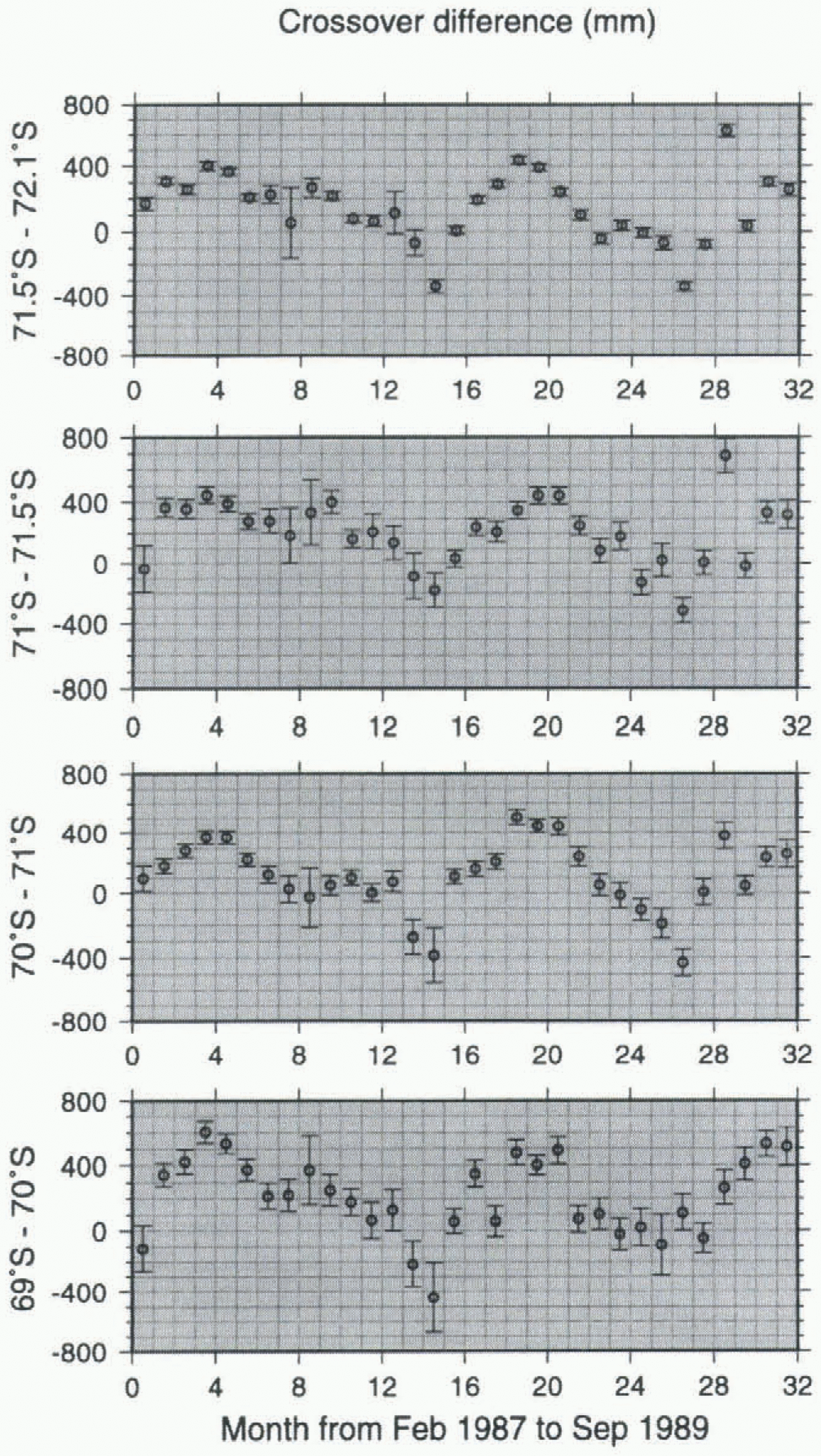
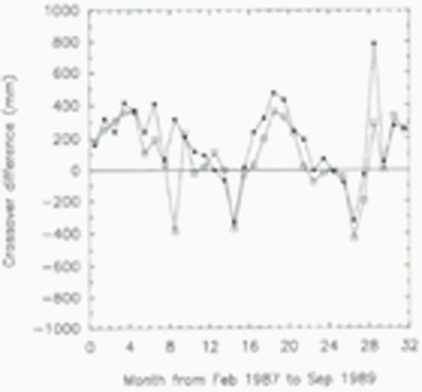
Crossover differences calculated between paths for the first 3 months and for each month thereafter; the elevation changes as a function of time are plotted. Each plotted value is a monthly average between, longitudes 80∘ and 140∘ E on the latitude band marked. The numbers on the abscissa denote the time in months from 1 February 1987. Thus the first interval represents February 1987, and the first plotted points are the averages for that month. Error bars are standard errors of the mean. 76470 crossover points were used in calculating these results.

three were compared to the average elevations for the first 3 months through a crossover method. The crossover differences were then averaged for each month over different latitude bands. Crossover differences with magnitude ?5 m (about 5% of the total) were rejected. Surface elevation as a function of time for four different latitude bands was then plotted (Fig. 4).

Secular variation

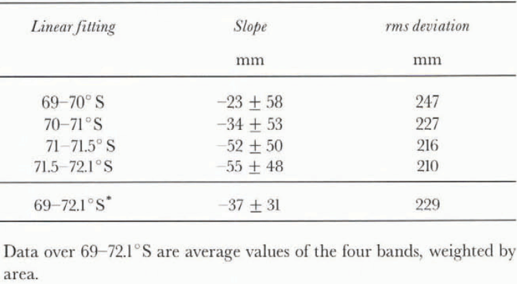
Evidence of a secular change in the average surface elevation was sought by applying linear regression analysis to the time sequences of crossover-difference data shown in Figure 4. The slopes of the fitted lines and their rms deviations are shown in Table 1. The slopes, which represent

Table 1.

Linear regression result of crossover differences in four bands in Figure 4

3 year estimates of a long-term linear trend, are not significantly different from zero. Furthermore, the strong quasiseasonal variations would mask completely any secular trend even if they were real, which they probably are not (see Discussion below).

Biases

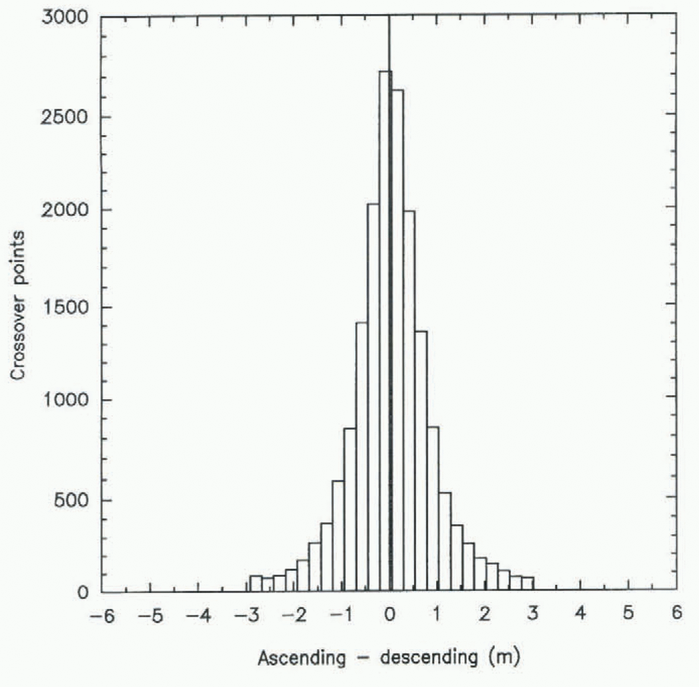
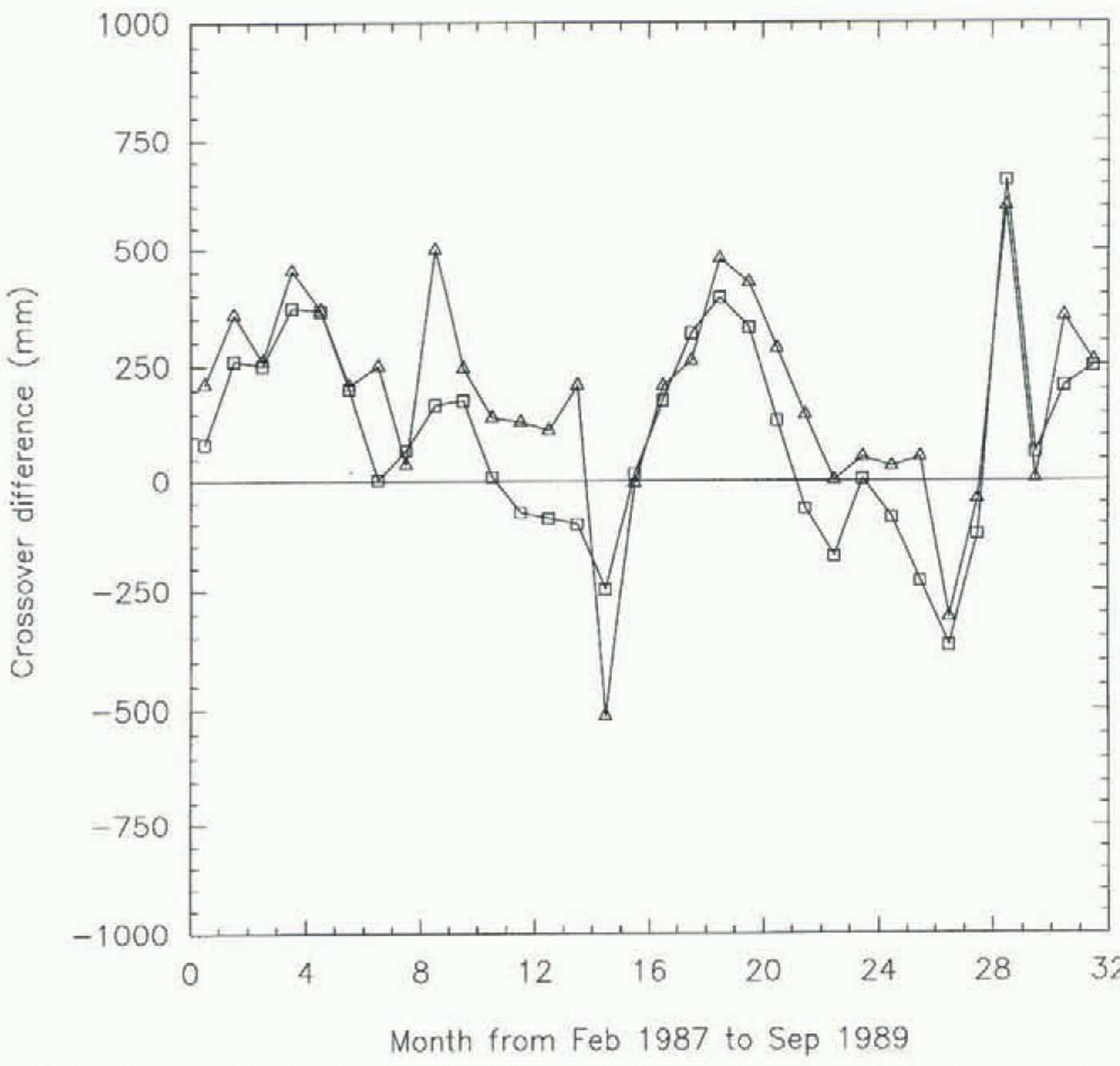
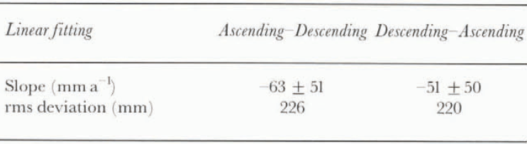
Crossover differences for ascending and descending paths during the same month were calculated for the 35 months to test for an ascending/descending bias. There are 17 623 crossover points in this calculation. Crossover differences larger than 5 m were again discarded. The histogram in Figure 5 shows an insignificant bias of 0.05 m between the ascending and descending paths (the standard deviation is l m). As another check against bias, linear trends were calculated separately from ascending–descending and descending–ascending crossover differences in the region 71.5–72.1°S, 80–140° E. The resulting surface elevations vs time

Fig. 5.

Histogram of ascending-minus-descending crossover differences for the same month for all 35 months of ERM data. Mean = 0.05 m, standard deviation = 0.99 m, 17 623 crossover points. Only crossover differences between ±f3σ were plotted.

are shown in Figure 6, and the corresponding linear regression results are in Table 2. The difference between the two is not significant.

We compared our retracking result to the result obtained by applying NASA’s retracking method. The histogram of crossover differences using data retracked by NASA’s method but applied only to the same waveforms as used to produce Figure 5 is essentially identical to that using our retracking method. (Our model corrects for the seasonal

Fig. 6.

Crossover differences calculated between paths for the first 3 months and each month thereafter over the band 71.5–72.1° S between 80° and 140° E. The numbers on the abscissa denote the time in months from 1 February 1987. Thus the first interval represents February 1987, and the first plotted points are the averages for that month. Squares: ascending minus descending; triangles: descending minus ascending.

Table 2.

Linear regression result of crossover difference in Figure 6

variation in penetration, which has an amplitude of about 0.2 m (Yi, 1996), but since the crossover points were calculated from paths during the same month, seasonal changes in penetration do not affect the result.) However, when we applied NASA’s retracking to all points that it would accept, the standard deviation increased from about 1 m to 1.6 m, a 60% increase. This presumably occurs because our model accepts only the better-shaped waveforms for retracking. In the region 71.5–72.1° S, 80–140° E, our model yields 1.87 x 10⁶ data points, whereas the NASA model gives 2.29 x 10⁶ data points.

Discussion

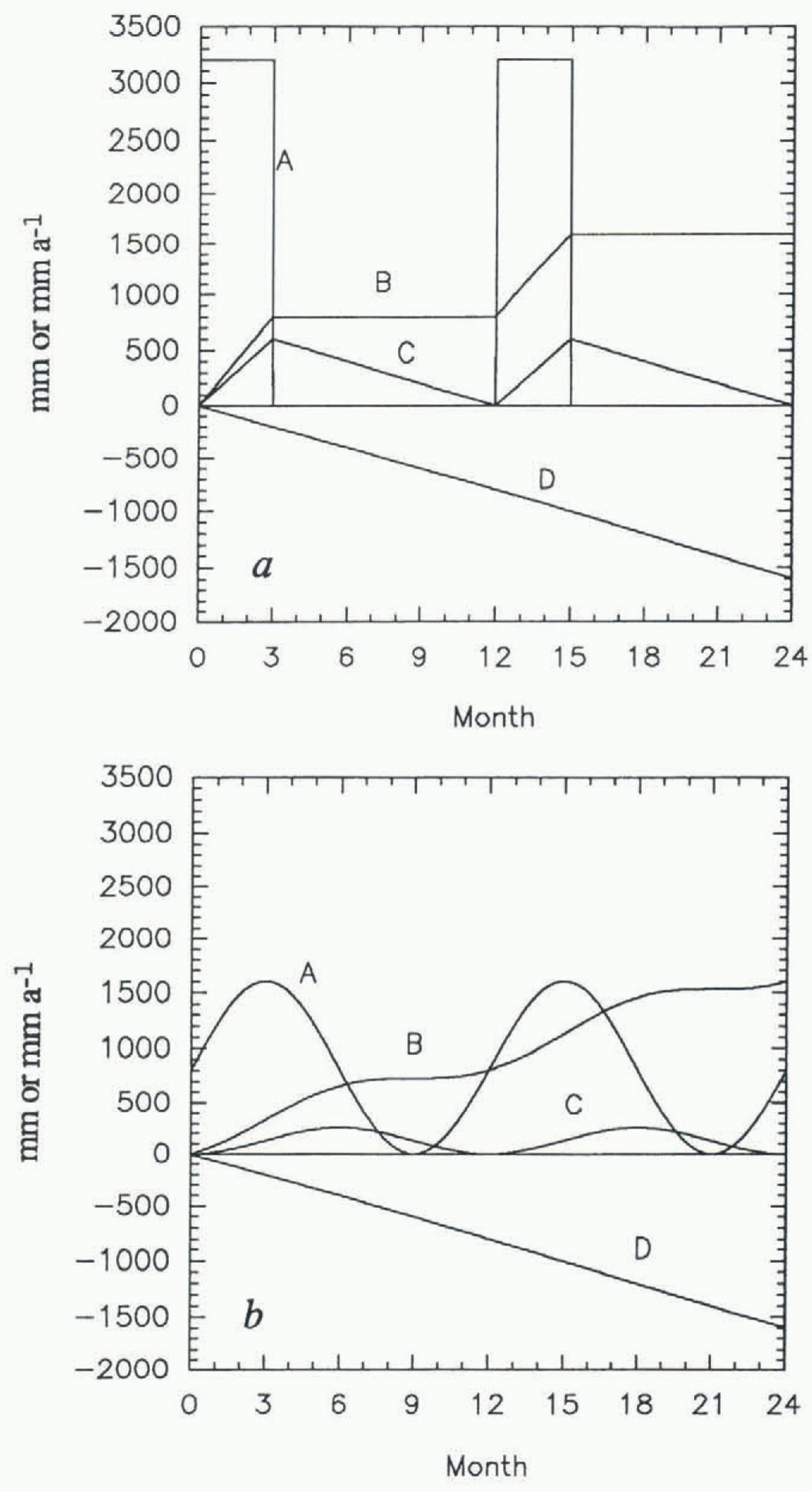
The amplitude of the periodic height change is about 600 mm, in a region where the mean annual accumulation rate is about 160 kg m^–2 a^–1 (160 mm w.e.a^–1) according to Young and others (1982). Such a large amplitude is not easy to explain, as can be seen from the following calculations. Assuming a near-surface density of 0.4 Mg m^–3, the average annual accumulated layer thickness according to Young and others (1982) should be 400 mm. If the region is in mass balance (i.e. no change in yearly averaged elevation), a particular horizon near the surface will move downward at a constant rate equal to the mean annual accumulation rate of snow (at this point we ignore densification; we consider it later). Suppose first that the accumulation rate during 1986–89 was the same as the long-term average. Let snow fall at a constant rate for 3 months, with no snowfall the rest of the year. In order to have an annual surface elevation cycle with an amplitude of 600 mm, the peak accumulation rate needs to be 3200 mm a^–1, which amounts to an annual average accumulation rate of 800 mm a^–1 of snow (Fig. 7a), twice as much as reported by Young and others (1982). If, more reasonably, the snowfall follows a sinusoidal pattern, then for the same yearly accumulation rate as in figure 7a, the yearly cycle in surface height (Fig. 7b) is only about half as much as in figure 7a, i.e. it would take an accumulation rate of 1600 mm a^–1 (snow) to produce the observed cycle.

Next, suppose that the long-term average accumulation rate is that given by Young and others (1982), but that the accumulation rate during 1986–89 was abnormally high. Lines D in Figure 7 would now slope downward at only 100 mm a^–1, not 800 mm a^–1. Consequently, curves C would now be tilted upward at a mean slope of 400 mm a^–1, meaning that the rectangular-wave model of figure 7a would imply a mean surface height increase of 400 mm a^–1, whereas the sine-wave model of figure 7b would necessitate a mean surface height increase of 1.2 m a^–1! Figure 4 shows immediately that there is no such height increase, so this model can be rejected.

Finally, we drop the assumption of long-term mass balance, but retain the average accumulation rate of Young and others (1982). The rates of surface height increase Calculated

Fig. 7.

A, modeled accumulation rates in mm a^–1; B, net surface balance in mm; D, elevation of the horizon that marks the surface at time 0; and C, the surface elevation (the sum of B and D). The snowfall follows (a) a rectangular pattern; (b) a sinusoidal pattern. The numbers on the abscissa denote the elapsed time in months.

in the previous paragraph now give the rates at which the surface would have had to be lowering during years of normal accumulation in order to show no change during the abnormally high-accumulation years, 1986–89. Rates of lowering of as much as 1 m a^–1 are known elsewhere in Antarctica (Shabtaie and others, 1988; Nishio and others, 1989), but only in association with highly active ice streams or outlet glaciers. This model is unappealing a priori, because a coincidental canceling of two independent signals with large, equal amplitudes and opposite signs is inherently extremely unlikely; furthermore, Bentley and Sheehan (1992) showed from Seasat and Geosat radar altimetry that the surface height change in the same region of East Antarctica was less than 0.2 m a^–1 between 1978 and 1987. We can reject this model also.

Because of the difficulty in explaining the large amplitude of the height variations in terms of real accumulation

Fig. 8.

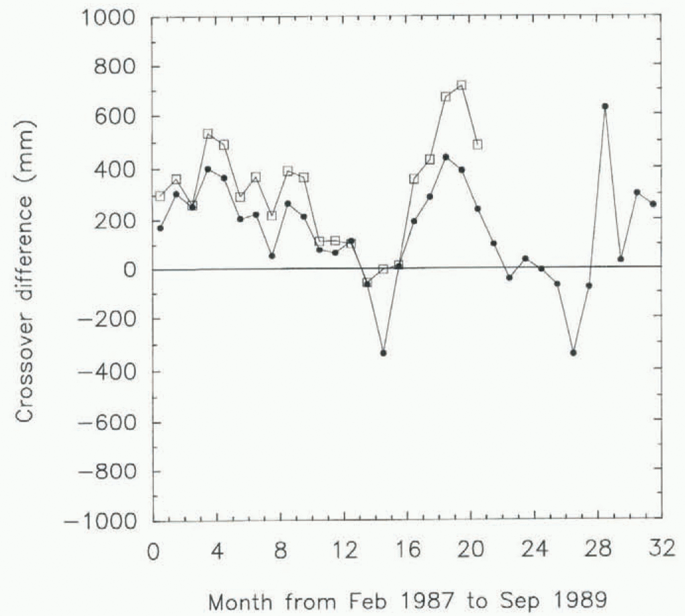
Elevation differences as a function of time in the latitude band 71.5–72.1° S separated into western (80–110° E; circles) and eastern (110–140° E; squares) halves. The numbers on the abscissa denote the time in months from 1 February 1987. Thus the first interval represents February 1987, and the first plotted points are the averages for that month.

rates, we have applied another test that takes into account the large difference in accumulation rate across our region. That difference is indicated clearly in the analysis by Budd and others (1995) of accumulation rates from moisture fluxes. According to that analysis (Budd and others, 1995, Fig. 3a) the accumulation rate should vary from less than 50 kg m^–2 a^–1 in the southwest corner of our area to some 600 kg m^–2 a^–1 at 69° S, 120° E, near the northeast corner. With such a large change in the accumulation rate one would expect a pronounced southwest–northeast gradient in the seasonal height changes if they were due to variations in accumulation. No such effect, or at most a very weak one, appears between the different latitude bands (Fig. 4). As a further check we have divided each latitude band into two halves and calculated results separately between longitudes 80° and 110° E and between 110° and 140° E. The accumulation rate given by Budd and others (1995) is two to three times greater in the more easterly half of each latitude band, so again one would expect a much larger seasonal variation in the eastern half of each band than in the western half. Instead, the patterns in the two halves are essentially identical (Figure 8 shows the comparison for the 71.5–72.1° S band). The fact that the apparent seasonal variation is completely independent of the total accumulation rate argues strongly against real seasonal variations in accumulation constituting more than a minor fraction of the observed signal.

All these difficulties and inconsistencies lead us to conclude that the apparent height variations either are not real at all or are principally due to some factor other than changes in the accumulation rate.

Consequently, we next seek possible sources of apparent change in height over a stationary surface. One conceivable source would be in the corrections that are applied to the travel time of the radar pulse to account for delays through the troposphere and the ionosphere. In the troposphere in the interior of Antarctica there are seasonal cycles of temperature (amplitude about 30°C (Stearns and others, 1993)) and mean atmospheric pressure (amplitude about 20 mbar (Steams and others, 1993)). These quantities, entered into the expression for the dry tropospheric correction that is applied to the Geosat data (Tapley and others, 1982), yield about 45 mm, which represents the magnitude of the seasonal variation in the applied correction. This is too small to point to an error here as the primary contributor to the indicated height change; the correction applied could hardly be in error by an order of magnitude.

In the case of the ionosphere, the relative change from summer to winter (i.e. sunlit to dark) is large, but the total correction is a maximum of only about 100 mm near the solar activity maximum (1989) and much less in 1987 (Musman and others, 1990; personal communication from A. Brenner, 1996); it seems highly unlikely that the correction could be in error by tens of centimeters (personal communication from D. Bilitza, 1996).

Another source to consider is orbit error. Generally speaking, orbit error is the largest source of uncertainty in calculating surface heights from radar altimetry in the polar regions; it arises principally from the extrapolation of orbits beyond the coverage or tracking stations using geopotential models that are themselves poorly constrained near the poles. However, these models (GEM-T2, in our case) are not functions of time. Significant sources of a seasonal variation in the orbit error are not obvious. Errors at the tracking station could arise from the same sort of atmospheric-delay factors already discussed, but error analyses over the ocean limit this source to a few tens of millimeters (Wagner and Cheney, 1992). Atmospheric drag could vary seasonally, but the effect of atmospheric drag is small; Wagner and Cheney (1992) show that it is less than 40 mm at lower latitudes. Since the upper atmosphere is even thinner

Fig. 9.

Elevation differences in the entire latitude hand 71.5–72.1° S based on orbits calculated, respectively, from the gravitational models GEM-T2 (circles) and JGM-2 (squares). The numbers on the abscissa denote the time in months from 1 February 1987. Thus the first interval represents February 1987, and the first plotted points are the averages for that month. Orbits based on JGM-2 are not available for the last year of the ERM.

Table 3.

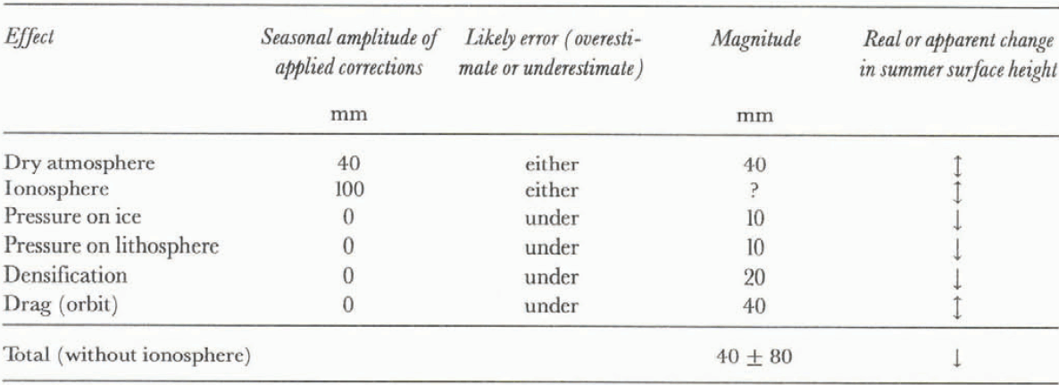
Factors that affect surface elevation

in the polar region, an error large enough to affect our result is unlikely.

To examine the likelihood of orbit error further, we have recalculated all our results for the first 2 years using orbits calculated from the JGM-2 gravitational model. JGM-2 is a major improvement over GEM-T2 because it includes the geoidal data available from TOPEX/POSEIDON radar altimetry. The 1 σ predicted orbit error is only 22 mm for JGM-2, compared with 102 mm (Nerem and others, 1995). To compare results using the two models close to Antarctica, A. Brenner (personal communication, 1996) calculated crossover differences as a function of time over the ocean south of 60° S in the same longitudes as our studies over the continent. She found variations of several tenths of a meter using GEM-T2 orbits, whereas the variations were mostly less than 0.1 m using JGM-2. In neither case were the variations periodic or correlative with those we observed.

Using JGM-2 instead of GEM-T2 yielded no significant change in our results. Variations over the first 2 years are similar (an example for the 71.5–72.1° S band is shown in Figure 9); using JGM-2 does not eliminate the quasi-seasonal variations; if anything, it makes them larger. Note, however, that differences between the two models (Fig. 9) reach several tenths of a meter. This clearly indicates that the predicted orbit errors cited above are far too small for the southernmost parts of the orbits. We believe these comparisons indicate that orbital errors of several tenths of a meter probably still remain over Antarctica, even with the best gravitational models yet available. Even though we have found no explanation for seasonal changes in the orbit error, we believe that orbit error remains a major problem.

Next, we consider effects in the ice sheet itself that might produce real variations in surface height. We note first that any seasonal variations in surface roughness and the depth of penetration should be compensated for by our retracking procedure, to the extent that our model fits the real process. Since the maximum seasonal variation in the elevation correction that we observed was only 0.2 m, and that number is not likely to be in error by a factor of 4 or 5, as would be needed to explain the indicated height changes, we discount variable penetration as an important contributor to the seasonal signal.

The seasonal variation in atmospheric pressure will cause a change in the total thickness of the ice sheet owing to differential compression. If we assume as an upper limit a mean porosity of 10% for the whole ice sheet below pore close-off (slow pressure changes will not compress the interconnected pores in the firn), the incompressibility would be about 6.6 GPa (66 kbar) (Röthlisberger, 1972, p. 17, equation 24). The 20 mbar summer/winter pressure difference then leads to a thickness difference of 10 mm, which is too small to matter.

The seasonal variation in the densification in the uppermost firn because of seasonal temperature differences and the exponential dependence of compaction rates on temperature (Bader and Kuroiwa, 1962) has also been estimated. We employ an empirical model of Herron and Langway (1980), which was developed using data from Greenland and Antarctica, including South Pole and Vostok in East Antarctica. For the low-density snow near the surface, their model gives

where T is the temperature in K, A is the accumulation rate in meters of water per year, ρ _i is the density of ice, and ρ is the density of the near-surface firn. (In Herron and Langway’s (1980) equation, A has an exponent, but the numerical value of that exponent is essentially 1.) We next suppose that the mean temperature in the uppermost 5 m of firn is 30° C warmer in the summer half of the year than in the winter half. (Below that depth the temperature differences are not only small but partly out of phase.) Using a mean annual temperature of –40°C and a near-surface density of 400 kg m^–3 leads to densification rates of 6.4 kg m^–3 a^–1 (1.6% per year) for the summer and 3.2 kg m^–3 a^–1 (0.8% per year) for the winter. Applying this to the 5 m column yields a total thinning of 40 mm for the summer half-year and 20 mm for the winter half-year, a difference of only 20 mm. The calculated total for the year is 60 mm, some 25% of the equilibrium compaction thinning of the entire firn layer, so this number can hardly be an underestimate. We conclude that this effect, like the others we have examined, is inadequate to explain the observations.

Finally, we examine the “inverted barometer” effect that arises from changing loads on the Earth’s surface associated with barometric pressure differences. The magnitude of this effect was found by MacMillan and Gipson (1994) to be about 0.5 mm mbar^–1 for continental sites not near a coast. Applying this coefficient to the mean seasonal pressure difference of 20 mbar already cited yields a height change on the order of 10 mm, again an order of magnitude too small to be important.

Even taken all together (table 3), the effects we have considered are not nearly adequate to explain the observed quasi-seasonal variation in surface height of the ice sheet. We must have either seriously undervalued or totally overlooked some disturbing factor or factors. Our suspicion rests strongly on orbit error as the culprit, but we have no “smoking gun”.

We note finally that the uncertainty in the source of the seasonal variation renders the estimates of a long-term trend meaningless.

Conclusion

A model for retracking satellite radar-altimeter waveforms that considers both surface and volume scattering has been developed and applied to data from the Geosat ERM to calculate surface elevations on a substantial section of the East Antarctic ice sheet. Using the mean indicated surface height from the first 3 months as a datum, the relative heights for each month thereafter were calculated by a crossover method. There is strong evidence for a pronounced seasonal cycle in the apparent height of the surface that is over 0.5 m in amplitude. Analysis of this height cycle in terms of the magnitude and distribution of accumulation rates in the region shows it to be unlikely that more than a small fraction of the observed changes results from real seasonal variations in the snow-accumulation rate. We believe orbit error probably is the most important contributor to the apparent changes, although we can suggest no likely source of such a large seasonal component of orbit error. Various other factors may contribute in a minor way, but none seems capable of producing an effect measured in tenths of meters.

The large quasi-periodic variations of uncertain origin preclude observing any moderate secular changes. However, there is clearly no dramatic secular increase or decrease in the surface height, such as would be associated with a major mass imbalance.