1 Introduction
One of the main challenges reinforcement learning (RL) (Sutton & Barto, Reference Sutton and Barto1998) faces is dealing with the sparsity of rewards that is present in many tasks. An RL agent will only very slowly learn to solve a task through trial and error if the feedback it receives in the form of rewards is given sparsely. This lack of feedback, and thus gradient, makes the agent explore the task uniformly at random, unless special mechanisms are implemented that guide the agent’s exploration.
One way of tackling this problem that is often taken is to include prior (heuristic) knowledge that can bias the agent towards what are a priori believed to be good states, or good behaviour. Prior knowledge can come in the form of rules defined by a domain expert (Togelius, 1994), demonstrations provided by such an expert (Schaal, Reference Schaal1997), prior learning experiences of the agent in different tasks (Taylor & Stone, Reference Taylor and Stone2009), so on.
Conversely, a second stream of thought, orthogonal to the former, tries to leverage internal knowledge and experiences in the current task to generate internal rewards to bias exploration in the absence of immediate external rewards. Approaches relying on intrinsic motivation (Bellemare et al., Reference Bellemare, Srinivasan, Ostrovski, Schaul, Saxton and Munos2016; Pathak et al., Reference Pathak, Agrawal, Efros and Darrell2017) attempt to leverage the ideas of curiosity and uncertainty to achieve more intelligent and effective ways of exploration.
This paper falls in the second category, as we develop a technique that allows the agent to bias its exploration by generating internal shaping rewards based on its own successful previous experiences in the task.
We evaluated our approach in the 4-dimensional CartPole domain and the 27-dimensional Super Mario AI domain, and the results show significant improvements in learning performance both when intrinsic RL is used on its own and when it is used in combination with human expert advice.
2 Background
In this section we introduce the background knowledge that underpins the work presented in this paper.
2.1 Reinforcement learning
RL (Sutton & Barto, Reference Sutton and Barto1998) is a paradigm that describes how an agent can improve its behaviour based on reward and punishment received from interactions with its environment. Maximizing the rewards accumulated over time equals solving the task by definition. We define an RL problem as a Markov Decision Process (MDP) 〈S, A, T, γ, R〉. S defines all environment states that can be observed, and A defines the actions an agent can take to affect this environment. T describes the dynamics of the system, defining the probability of the environment transitioning from state s to state s′, given that action a was taken: T(s′|s, a). R is the reward function that yields a numerical reward for every state transition, defining the task. Finally, γ is called the discounting factor and defines how important long-term rewards are, that is, how short- or far-sighted the agent is.
The goal of an RL agent is to find behaviour, that is, a policy π : S → A that maximizes the expected accumulation of rewards. Many approaches do not directly search the policy space, but instead estimate the quality of actions in each state, and derive a policy from these estimates. The quality of states and actions is defined by the Q-function: Q : S × A → ℝ. Temporal difference algorithms, such as Q-learning (Watkins, Reference Watkins1989), approximate the true Q-function by incrementally updating their estimates:
 $$Q(s,a) \leftarrow Q(s,a) + \alpha \delta $$
α is the learning rate, and δ is the temporal-difference error, the difference between the previous estimate and the target being tracked:
 $$\delta = R(s,a,s') + \gamma \mathop {\max }\limits_{a'} {\rm{ }}Q(s',a') - Q(s,a)$$
Q-learning is guaranteed to converge to the true Q-values, and thus an optimal policy, given certain assumptions such as a decreasing learning rate (Tsitsiklis, Reference Tsitsiklis1994).
2.2 Reward shaping
Vanilla versions of model-free RL algorithms typically require excessive amounts of interactions with the environment to learn high-quality policies, because they do not incorporate prior knowledge to guide exploration. They must therefore rely on uniformly random exploration of the state–action space in order to stumble on the typically sparse rewards. Only after enough state transitions and their associated rewards have been observed can the agent start to exploit this knowledge by biasing its action selection towards what its estimates indicate are good actions. Incorporating prior knowledge to bias initial exploration is a successful way of reducing learning time in RL, the most notable recent example being AlphaGO using expert demonstration data (Silver et al., Reference Silver, Huang, Maddison, Guez, Sifre, Van Den Driessche, Schrittwieser, Antonoglou, Panneershelvam and Lanctot2016).
Reward shaping, derived from behavioural psychology, is a popular way of including prior knowledge in the learning process in order to alleviate the random exploration problem. It provides a learning agent with extra intermediate rewards, like a dog trainer would reward a dog for completing part of a task. This extra reward can enrich a sparse base reward signal (e.g., a signal that only gives non-zero feedback when the agent reaches the goal), providing the agent with useful gradient information. This shaping reward F is added to the environment’s reward R to create a new composite reward signal that the agent uses for learning:
 $$R_F (s,a,s') = R(s,a,s') + F(s,a,s')$$
Of course, since the reward function defines the task, modifying the reward function may modify the total order over policies and make the agent converge to suboptimal policies (with respect to the environment’s reward alone).
Following Ng et al. (Reference Ng, Harada and Russell1999), we define a potential function Φ : S → ℝ over the state space and take the reward shaping function F as the difference between the new and old states’ potential. Doing that provably maintains the total order over policies and preserves any convergence guarantees (Ng et al., Reference Ng, Harada and Russell1999):
 $$F(s,a,s') = \gamma \Phi (s') - \Phi (s)$$
Prior knowledge can be numerically encoded in the potential function Φ. The effect of applying such reward shaping, which is typically denser than the sparse environment reward, is that the agent is more likely to encounter non-zero rewards, and thus its exploration will move away from uniform random much earlier in learning. Instead, it will be biased towards states with high potentials. For example, using height as a potential function in Mountain Car (Singh & Sutton, Reference Singh and Sutton1996) biases the agent to selecting actions that will increase height. Since the goal location in Mountain Car lies on top of a hill, shaping using this heuristic helps an agent solve that task faster.
The definition of F and Φ was extended by others (Wiewiora et al., Reference Wiewiora, Cottrell and Elkan2003; Devlin & Kudenko, Reference Devlin and Kudenko2012; Harutyunyan et al., Reference Brys, Harutyunyan, Suay, Chernova, Taylor and Nowé2015) to include actions and time steps, allowing for the incorporation of behavioural knowledge that reflects the quality of actions as well as states, and allowing the shaping to change over time:
 $$F(s, a, t, s', a', t') = \gamma \Phi (s', a', t') - \Phi (s, a, t)$$
These extensions also preserve the total order over policies and therefore do not change the task, given Ng’s original assumptions.
2.3 Reinforcement learning from demonstration
Reinforcement learning from demonstration (RLfD) is a term coined by Schaal (Reference Schaal1997) to denote the intersection between the fields of RL and learning from demonstration (LfD). As in RL, an agent operating in an LfD setting looks for a policy π that allows it to execute a task (Argall et al., Reference Argall, Chernova, Veloso and Browning2009). While in RL, the agent has a reward signal to evaluate behaviour, this objective evaluation metric is not present in the LfD setting (similarly for inverse RL (Ng et al., Reference Ng, Andrew and Russell2000; Suay et al., Reference Suay, Brys, Taylor and Chernova2016) and the agent must refer to expert demonstrations (sequences of state–action pairs {(s 0, a 0), …, (s n, a n)}) of the task to derive a policy that mimics and generalizes these demonstrations. This constrains the LfD agent to the behaviour the expert demonstrator exhibits (however good or bad) (Argall et al., Reference Argall, Chernova, Veloso and Browning2009). On the other hand, LfD agents are typically much more sample efficient than RL agents, requiring orders of magnitude less demonstrator samples than an RL agent needs environment interactions to learn good behaviour.
An RLfD agent, possessing both an objective reward signal and demonstrations, is able to combine the best from both fields, leveraging demonstrations to direct what would otherwise be uniform random exploration and thus speed up learning, while leaving the theoretical guarantees associated with RL in place, as the objective reward signal allows such an agent to eventually outperform a potentially suboptimal demonstrator.
Schaal (Reference Schaal1997) proposed two basic approaches for using demonstrations in an RL setting that were later developed by other researchers. One is the generation of an initial value-function for Q-learning by using the demonstrations as passive learning experiences for the RL agent. This was later built upon by Smart & Kaelbling (Reference Smart and Kaelbling2002). The other approach derives an initial policy from the demonstrations and uses that to kickstart the RL agent. This approach was picked up and further developed in Taylor et al. (Reference Taylor, Suay and Chernova2011), Brys et al. (Reference Brys, Harutyunyan, Suay, Chernova, Taylor and Nowé2015) and Suay et al. (Reference Suay, Brys, Taylor and Chernova2016). In this paper, we mainly build upon and compare with the demonstration reward shaping work from Brys et al. (Reference Brys, Harutyunyan, Suay, Chernova, Taylor and Nowé2015).
In that work, demonstrations are encoded as a reward shaping function by defining a Gaussian similarity measure over the state space:
 $$g(s,s^d ,\Sigma ) = e^{( { - {1 \over 2}(s - s^d )^T \Sigma ^{ - 1} (s - s^d )})}$$
and subsequently incorporating it in the potential function as follows:
 $$\Phi (s,a) = \mathop {\max }\limits_{(s^d ,a)} g(s,s^d ,\Sigma )$$
thus creating a Gaussian landscape that rewards the agent for mimicking the demonstrator, but allows it to deviate from the demonstrator’s example as well.
3 Principles of introspective RL
This section will describe the methodology of using the agent’s own experiences to shape the reward function in order to bias exploration and speed up RL. Typically, in complex environments, rewards must be observed many times before the agent acquires a significant behavioural bias towards pursuing those rewards. In the introspective RL approach we propose, we leverage these experiences to include a more explicit bias, by shaping the reward function, rewarding current behaviour that is similar to past behaviour that led to rewards. A different perspective on this is to say that those previous experiences that led to rewards are task demonstrations (provided by the agent itself), which can be used to bias the agent’s current exploration in the same fashion as external expert demonstrations would be used as described above in Section 2.3. If actual external expert demonstrations are available, these could even be used to initialize the introspective agent’s bias.
3.1 Collecting the experiences
Introspective RL extends RL by adding an experience filter module and addresses the reward sparsity problem using dynamic reward shaping based on the filtered experiences. The experience filter collects the agent’s exploratory behaviour that led to positive outcomes into a priority queue. These experiences are then immediately used as an exploratory bias to speed up the learning process.
Specifically, during a learning episode, every state–action–next state-reward tuple ((s t, a t, s t+1, r t)) is stored in memory. At the end of the episode, the Q-value  $\widehat {q}(s_{t}, a_{t})$ for each state–action in this episode is Monte Carlo estimated until the final time step T:
 $$\widehat {q}({s_t},{a_t}) = \sum\limits_{k = t}^T {{\gamma ^{k - t}}} {r_t}$$
The state–action pairs and their estimated Q-values are then stored in a priority queue with the estimated Q-values being the sort key of the queue. If the queue is full (defined by queue size parameter qs), only state–action pairs with a higher estimated Q-value than the smallest in the queue are added (and the smallest are consequently removed). If the queue is not full, all state–action pairs and their estimated Q-value are added.
Progressively, poorer Q-value elements of the queue will be removed, and experiences with higher estimated performance levels will remain. Thus, the exploratory bias induced by these experiences will progressively increase in quality.
Introspective RL is using prior experience to compute a reward shaping function, rather than using it to replay past experience directly (Schaul et al., Reference Schaul, Quan, Antonoglou and Silver2015). As such, our approach is closer to the automatic generation of a reward shaping function. Also, our approach does not depend on using poor performing actions in the priority queue, which is sorted by Q value (and not Temporal Difference (TD) error as in prioritized experience replay). Furthermore, dynamic reward shaping (Devlin & Kudenko, Reference Devlin and Kudenko2012), as applied to experience reuse in our approach, has been proven to conserve the convergence guarantees of the RL algorithm used, in our case Q(λ).
3.2 Defining the potential function
In the manner of Brys et al. (Reference Brys, Harutyunyan, Suay, Chernova, Taylor and Nowé2015), we encode state–action pairs as a potential function using a Gaussian similarity metric.Footnote 1 The assumption is that if in the agent’s past experience, certain state–action pairs led to high rewards, taking the same action in a similar state might lead to similarly high rewards.
When the potential function Φ(s, a) needs to be calculated in a certain state–action pair (s, a), first the agent must look in the priority queue for the recorded state–action pair that is most similar to the current, using Equation (2). Then the potential function is defined as follows:
 $$\Phi (s,a) = \rho \mathop {\max }\limits_{(s^d ,a)} g(s,s^d ,\Sigma )\widehat {q} (s^d ,a)$$
which is a modification of Equation (3), incorporating the actual estimated quality of that state–action pair  $\widehat {q}$ and a scaling factor ρ to control the strength of the exploratory bias induced. The update rule of introspective Q-learning is as follows:
 $$Q(s_t ,a_t ) \leftarrow (1 - \alpha )Q(s_t ,a_t ) + \alpha (r_t + F(s_t ,a_t ,t,s_{t + 1} ,a_{t + 1} ,t + 1) + \gamma {\rm{ }}\mathop {\max }\limits_b {\rm{ }}Q(s_{t + 1} ,b)$$
F(s t, a t, t, s t+1, a t+1, t + 1) is the reward shaping function defined in Equation (1), a gap of potential between current state–action and the nearest state–action in priority Q defined by Equation (2).
Since the agent progressively collects more and more experiences, in principle of higher and higher quality, the potential function will change from episode to episode, making this potential function a dynamic one. Note that theoretical guarantees, that is, that the optimal policy does not change, hold for dynamic potential-based advice (Harutyunyan et al., Reference Brys, Harutyunyan, Suay, Chernova, Taylor and Nowé2015), and that no modification to the policy needs to be made given that the initial Q-function is all zeroes.
3.3 Initializing the priority queue with demonstrations of external agents
Even though the introspective RL idea is focused on using the agent’s own experiences to bias its learning, it is also completely amenable to receiving an a priori-bias from demonstrations provided by an external agent. Such demonstrations can easily be incorporated by putting them through the same process of estimating Q-values and storing them in the priority queue as the experiences collected by the agent itself. When qualitatively good, these demonstrations can prevent the agent from initially filling the priority queue with whatever low-quality random trajectories it executes first, allowing it to be positively guided from the first episode.
Specifically, demonstration data from external agents will be collected as a set of episodes, that is, sequences of state–action pairs that terminate in an end-state. Monte Carlo estimation of the Q-value  $\widehat {q} ({s_i, a_i})$ is performed, and the individual state–action pairs, augmented with the estimated Q-value, are inserted into the priority queue. If the demonstration data do not include the reward signal, a viable solution may be to set the reward to 1 for all (s n, a n). The RLfD work we base ourselves successfully deals with this problem in the same way (Brys et al., Reference Brys, Harutyunyan, Suay, Chernova, Taylor and Nowé2015).
3.4 Pulling it together
The pseudo-code in Algorithms 1 and 2 describes a Q-learning agent employing the introspective technique to shape its exploration, showing how all components interact on an algorithmic scale.
Introspective Q-learning
 $\widehat { q _ { t } } \leftarrow \widehat { q _ { t } } + \gamma ^ { i } r _ { t + i }$
 $( \lt {s_t},\,{a_t},\,\widehat {q_t} > ,PQ)$
Filter high Q-value experience
 $( \lt {s_t},\,{a_t},\,\widehat {q_t} \gt ,PQ)$
 $\widehat {q_{t}}$>)
 $\widehat {q_{e}}$> ← the last element of PQ
 $\widehat{q}_{t} > \widehat {q}_{e}$ then
 $\widehat {q_{e}}$>) from PQ
 $\widehat {q_{t}}$>)
4 Experimental validation
Two domains, CartPole and Super Mario, were selected to demonstrate the strength of the proposed approach in this paper. Q(λ)-learning and RLfD (Brys et al., Reference Brys, Harutyunyan, Suay, Chernova, Taylor and Nowé2015) were used as benchmarks to be compared with the learning curve of the proposed approach. In CartPole and Super Mario, 10 and 20 trial demonstrations from human experts were used, respectively, to initialize the priority queue and shape the RLfD agent.
The results of all curves show the average of 30 runs and have passed a t-test. The t-test was conducted for every hundredth time step, and all the presented empirical results are statistically significant with p < 0.05.
4.1 CartPole
In the CartPole domain (Michie & Chambers, Reference Michie and Chambers1968), the RL agent controls a cart with a pole at its centre connected by a mechanical coupling. The RL agent learns to keep the pole balanced by pushing the cart to the left or the right. The observation consists of four features: the Cart’s velocity, its position, the angle of the pole and its angular velocity.
In the experiments, Q(λ)-learning and RLfD were used as the benchmarks to be compared to introspective RL with and without demonstrations, to show the advantages of introspection. We set all parameters following Brys et al. (Reference Brys, Harutyunyan, Suay, Chernova, Taylor and Nowé2015) with whose RLfD method we will compare: learning rate  $\alpha = \frac { 0.25 } { 16 }$ discount rate γ = 1.0, λ = 0.25 and an ∊-greedy exploration strategy with ∊ = 0.05. Tile coding was used as the function approximation with 16 10 × 10 tilings. Additionally, the potential function scaling parameter ρ = 0.2.
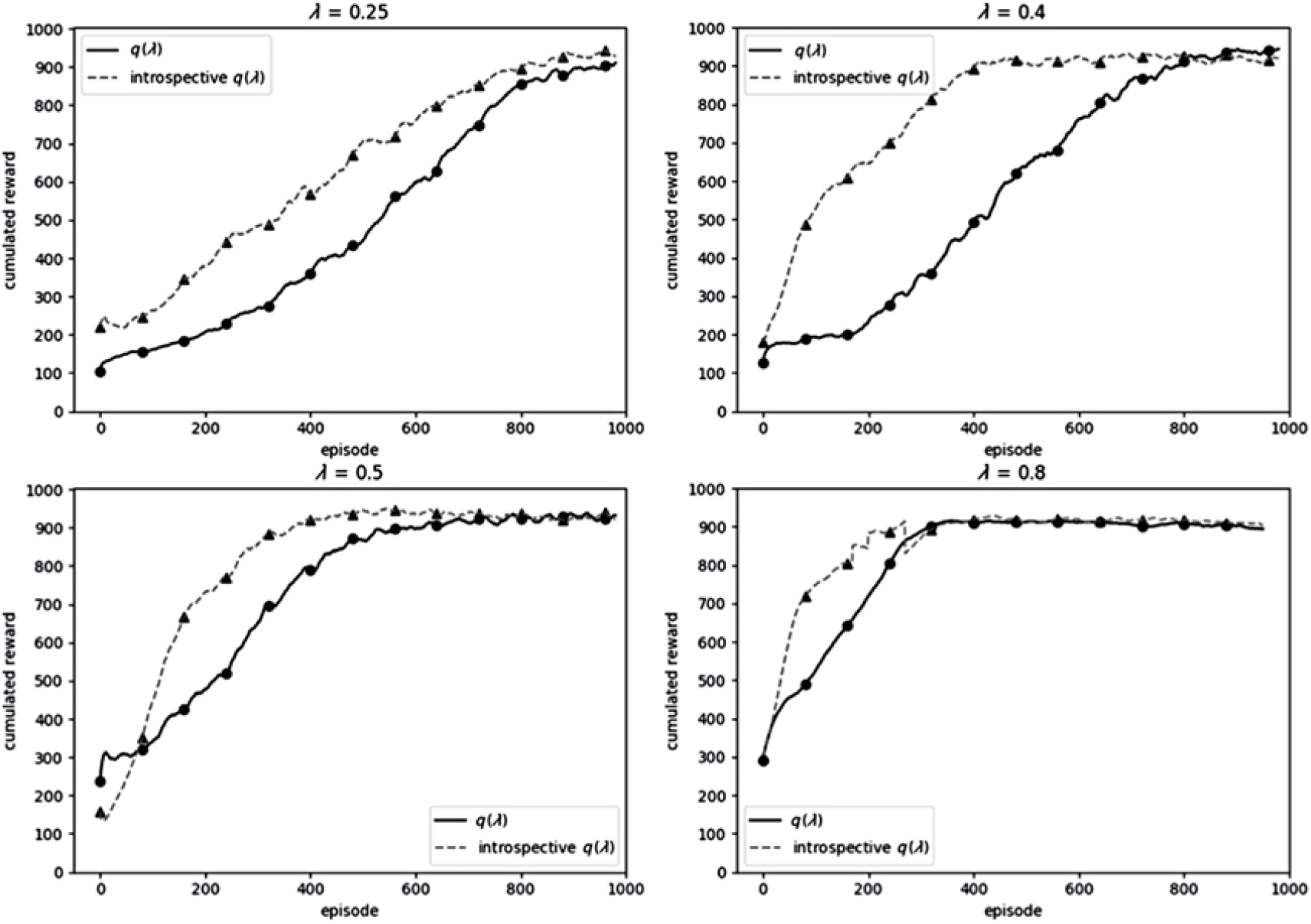
Figure 1 shows the results of comparing plain Q(λ)-learning with introspective RL (without demonstrations). While both methods converge to optimal behaviour, the results show that introspection leads the agent to learn significantly faster than the regular Q(λ)-learning agent. Since the λ parameter chosen in Brys et al. (Reference Brys, Harutyunyan, Suay, Chernova, Taylor and Nowé2015) and adopted by us is quite low, we show experiments with two higher λ ∈ {0.4, 0.8} in Figure 2. For higher λ, convergence for both methods is significantly faster, but the introspection advantage remains. In Figure 3, we show the effect of external demonstrations on the learning processes. We compare the baseline Q(λ)-learning without demonstrations, with the RLfD approach provided with 10 different demonstrations, and our introspective Q(λ) agent using the same 10 demonstrations to seed the experience queue. The external demonstrations have sub-optimal performance between 450 and 700 steps of keeping the pole up. The results show that while leveraging demonstrations can help, giving RLfD a jumpstart compared to the vanilla Q(λ)-learner and the introspective agent, the introspective agent very quickly outperforms both other agents. Since the use of demonstrations and the introspective mechanism are orthogonal to each other, we see here that they can be combined to provide a more powerful learner. Furthermore, the introspective mechanism will replace the potentially sub-optimal external demonstrations’ exploratory bias as the agent discovers better trajectories by itself. In the static RLfD case, the suboptimal bias remains throughout the learning process. Even though theoretical guarantees for convergence apply to both the dynamic introspective case and the static RLfD case, it is clearly better to dynamically change the bias to include higher and higher quality experiences.
CartPole learning curves of Q(λ)-learning and introspective reinforcement learning without any external demonstrations

CartPole learning curves of Q(λ)-learning and introspective reinforcement learning for λ ∈ {0.25, 0.4, , 0.5, 0.8}

CartPole learning curves of Q(λ)-learning, reinforcement learning from demonstration and introspective reinforcement learning with demonstrations

4.2 Super Mario AI competition benchmark
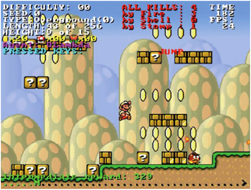
Super Mario Bros is a famous 2D side-scrolling video game first released by Nintendo in 1985. Karakovskiy & Togelius (Reference Karakovskiy and Togelius2012) converted this game into an AI algorithm competition benchmark as shown on Figure 4. The goal of the game is for the agent to maximize its points. Points are earned for collecting coins, killing enemies and finishing a game level, while points are subtracted for getting hurt and dying. The game ends when the agent is killed by an enemy, drops from a cliff, runs out of time or finishes the level. The RL agent’s reward corresponds to the points collected in the Super Mario game (e.g., for collecting coins or killing enemies) and to a large extent on being able to complete the level. Negative rewards are given for getting hurt by enemies or falling off a cliff.
A Super Mario screen shot

The actions available for the Mario agent correspond to the buttons on the original game controller, which are (left, right, no direction), (jump, don’t jump) and (run/fire, don’t run/fire). One action from each of these groups can be taken simultaneously, resulting in 12 distinct combined actions. We use the same state-space as described in Brys (Reference Suay, Brys, Taylor and Chernova2016), which involves 27 discrete state features:
1 is Mario able to jump? (Boolean)
2 is Mario on the ground? (Boolean)
3 is Mario able to shoot fireballs? (Boolean)
4–5 Mario’s direction in the horizontal and vertical planes ( {−1, 0, 1})
6–9 is there an obstacle in one of the four vertical grid cells in front of Mario? (Boolean)
10–17 is there an enemy within one grid cell removed from Mario in one of eight different directions (left, up-left, up, up-right, etc.) (Boolean)
18–25 as the previous, but for enemies within two to three grid cells (Boolean)
26–27 the relative horizontal and vertical positions of the closest enemy (( −10, 10), measured in grid cells, plus one value indicating an absence of enemies)
Similar to the CartPole domain, we used Q(λ)-learning and RLfD as benchmarks. The parameters were taken from Brys (Reference Suay, Brys, Taylor and Chernova2016), with the learning rate α = 0.001, discount factor γ = 0.9, ∊-greedy exploration with ∊ = 0.05, λ = 0.5 with the additional σ = 0.5 for RLfD.
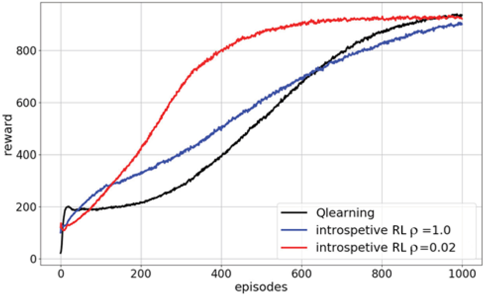
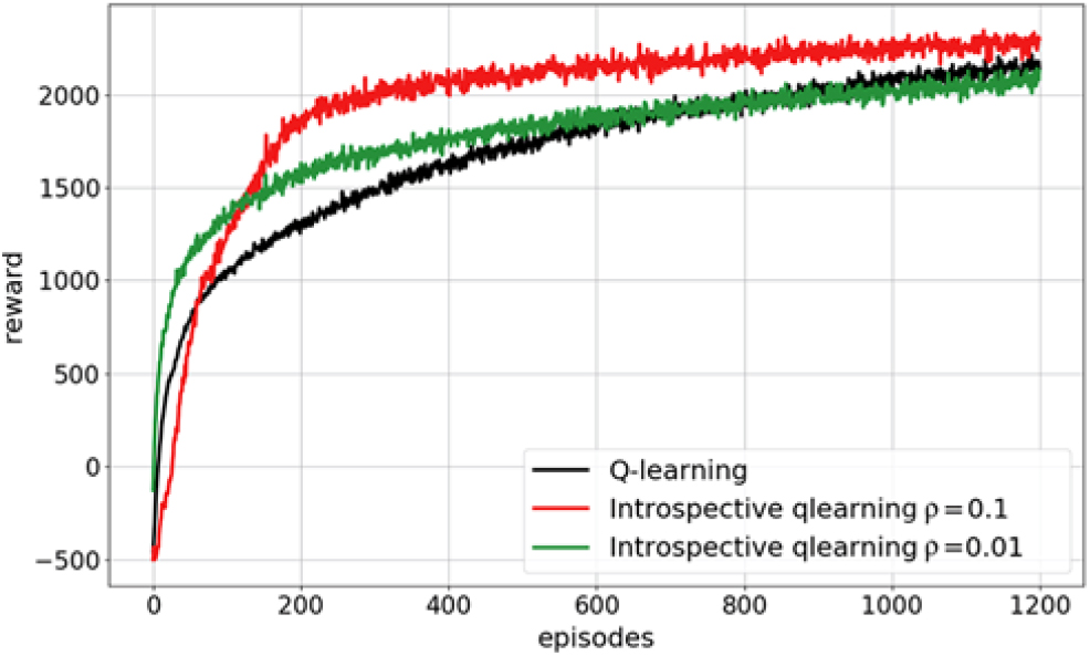
Figure 5 shows the learning curves of Q(λ)-learning and the introspective RL agent without demonstrations in the Super Mario domain. We show results for two different values of the potential function scaling factor ρ. The results are similar to the CartPole domain in that the learning performance of the introspective RL agent without demonstrations significantly improves over that of Q(λ)-learning and reaches the asymptotic performance level earlier.
Super Mario domain learning curves of Q(λ)-learning and introspective reinforcement learning without demonstration

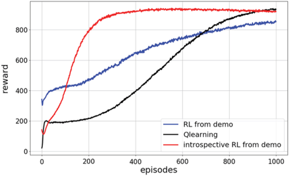
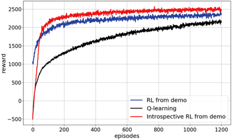
In another set of experiments, shown in Figure 6, 20 demonstration episodes from a human player (all with a performance score between 400 to 650) are used to initialize the priority queue for introspective RL. The results show that also in this highly complex domain, introspective RL with demonstrations outperforms both RLfD and regular Q(λ)-learning.
Super Mario Domain learning curves of Q(λ)-learning, reinforcement learning from demonstration and introspective reinforcement learning with demonstration

5 Conclusion and future work
In this paper, we presented the idea of introspective RL which takes inspiration from learning by demonstration. However, instead of using external expert demonstration to guide the learning, the RL agent uses its own experiences that have produced high rewards in the past. The agent keeps a priority queue to record the most successful experiences as tuples of the form 〈s, a,  $\widehat {q}$ 〉, where the Q value is obtained by Monte Carlo estimation. When the agent executes an action that is the same as the action of the most similar state in the priority queue, a reward based on the product of ρ,
 $\widehat {q}$ and the degree of similarity is added, where ρ is the hyper parameter that controls the weight of the reward shaping signal. Human experts’ demonstrations can be used by injecting the corresponding state–action–q triples into the priority queue. In this way, introspective RL can be complementary to RLfD.
We empirically evaluated our introspective RL approach on two domains, namely the CartPole domain with 4 continuous features and the Super Mario domain with 27 discrete features. The results showed that the introspective RL agent surpasses regular Q(λ)-learning performance significantly and reaches the asymptotic performance much earlier. Furthermore, introspective RL with demonstrations significantly improves performance in both domains compared to state-of-the-art RLfD. The empirical results also show that while introspective RL can use up more computational time per learning step, this loss is counterbalanced by a reduced sample complexity, which is generally more critical than computational complexity.
In future work, we intend to apply introspective RL to deep Q learning. For example, the similarity of parameters in high layers of the Q-value neural network may be considered to represent the similarity of state in a high-level concept and could be used for reward shaping. Another promising area of investigation is the optimization of the balance between the extra reward signals and the real rewards from the environment. A more sophisticated control of the parameter ρ (e.g., decay over time) could help to improve the learning performance.