


1 Introduction
Generally speaking, Fourier transforms exhibit an oscillatory behaviour, fluctuating between positive and negative values infinitely often. While the transforms of several cases of elementary functions are nonoscillatory, this should be viewed, rather, as an exceptional case. Furthermore, when dealing with nonoscillatory Fourier transforms, it appears that general results for determining the sign of the Fourier sine or cosine transform of a given real-valued function are currently lacking.
The issue of establishing the positivity (or the negativity) of a given Fourier transform is still an open question, and very few contributions can be found in the current literature (see, for example, [Reference Giraud and Peschanski6, Reference Tuck15]). In [Reference Tuck15], Tuck showed that every function strictly decreasing on
 $\mathbb {R}_0^+$
has an everywhere positive sine transform. He also proved that every function convex on
 $\mathbb {R}_0^+$
has a positive cosine transform for all
 $\omega> 0$
.
This paper focuses on establishing the positivity or negativity of a given Fourier sine or cosine transform, in general, only for suitably large values of
 $\omega $
, say
 $\omega> \omega _0$
, also providing an estimate for
 $\omega _0$
. Establishing the sign of a given sine or cosine transform only under such a restriction was envisaged in [Reference Tuck15]. We restrict to smooth functions and leave out the case of functions with integrable singularities.
It should be kept in mind that the plain positivity of a given function,
 $f(t)$
, is very different from its positive-definiteness. While the former property merely refers to the fact that
 $f(t)$
takes real positive values, a function
 $f:\mathbb {R}\rightarrow \mathbb {C}$
is called positive-definite if, for all real numbers
 $t_1,t_2,\ldots ,t_n$
, the
 $n \times n$
matrix
 $A := \{f(t_i - t_j)\}_{i,j}^n$
is positive definite, that is, for any real numbers
 $t_1,\ldots ,t_k$
and complex numbers
 $\xi _1,\ldots ,\xi _k$
, one has
 $\sum _{j,k=1}^n f(t_k-t_j) \, \xi _j \bar {\xi }_k \geq 0$
. Hermitian matrices have this property. It follows that it is necessary (but not sufficient) that such functions obey the conditions
 $f(0) \geq 0$
and
 $|f(t)| \leq |f(0)|$
.
Positive-definiteness is indeed encountered within the theory of Fourier transforms. By a theorem of Bochner [Reference Bochner4], the Fourier transform of a continuous positive function is positive-definite. However, positive-definiteness does not imply plain positivity.
In [Reference Giraud and Peschanski6], constraints and properties of real-valued functions with positive Fourier transforms were considered, motivated by various problems in physics and applied mathematics. In two dimensions, the positivity of the Fourier transform is relevant in particle physics, condensed matter physics, quantum chromodynamics and probability theory. In [Reference Giraud and Peschanski6], the authors used Hermite–Fourier functions and Sturm sequences to obtain constraints to ensure that a given function and its Fourier transform are both real-valued and positive. The method is constructive and based on the algebra of Hermite polynomials. However, it appears that this approach cannot be effectively applied in general cases. A connection with Bochner’s theorem was discussed and some simple analytic algorithms presented for checking positivity of the Fourier transform in some instances of positive functions. In [Reference Giraud and Peschanski9], the authors discuss more specifically positive Fourier transforms in the context of quantum chromodynamics.
Since, in some special cases, monotonicity of functions can play a role as in [Reference Tuck15], we note that in [Reference Boas2], the weighted Lebesgue integrability of the sine transform of monotonic functions was discussed. Earlier, in [Reference Boas and Kac3], several inequalities for the Fourier transform of nonnegative functions were established and some results for the zeros of such transforms were obtained.
In Theorem 2.1, we show that any suitably regular function,
 $f(t)$
, with
 $f(0) = 0$
but
 $f"(0) \neq 0$
, has a Fourier sine transform,
 $\mathcal{F}_S[f(t)](\omega )$
, with the opposite sign to
 $f"(0)$
, at least for
 $\omega>\omega _0$
, where
 $\omega _0$
can be estimated. The same result holds if
 $f(0) = f"(0) = \cdots = f^{(2k-2)}(0) = 0$
, while
 $f^{(2k)}(0) \neq 0$
for some given
 $k \in \mathbf {N}$
.
These outcomes have a counterpart for cosine transforms and derivatives of odd order: if
 $f'(0) = 0$
and
 $f"'(0) \neq 0$
, the cosine transform of
 $f(t)$
has the same sign as
 $f"'(0)$
and the same holds true if
 $f'(0) = f"'(0) = \cdots = f^{(2k-1)}(0) = 0$
, while
 $f^{(2k+1)}(0) \neq 0$
; if
 $f'(0) \neq 0$
, then the cosine transform has the opposite sign to
 $f'(0)$
, at least for
 $\omega $
sufficiently large (see Theorem 2.2). Unlike Tuck’s findings, these results do not rely on any assumption of monotonicity or convexity, although they generally hold only for sufficiently large values of
 $\omega $
.
As explained in Example 4.3, our theorems cannot explain the different behaviour of similar ‘bell-shaped’ functions, an issue deserving to be clarified, as pointed out in [Reference Tuck15]. In fact, such functions are even and hence their derivatives of all odd orders vanish at zero, so that we cannot infer anything on the sign of their cosine transform from Theorem 2.2.
Our proofs are in Section 2. In the short Section 3, we discuss the effects of a perturbation on the sign of the sine or cosine transform of a given function. A limited number of examples, mostly rather simple but illustrative, are given in Section 4. Several more examples are contained in a separate document of supplementary material. Some computations were performed using Mathematica [19].
2 Establishing the sign of Fourier sine and cosine transforms
The normalisation constants of the various Fourier integrals do not affect their sign and, hence, we will set them equal to one, unless explicitly stated otherwise. In some examples, we adopt the normalisations (see [Reference Abramowitz and Stegun1], [Reference Olver, Olde Daalhuis, Lozier, Schneider, Boisvert, Clark, Miller, Saunders, Cohl and McClain12, Tables 1.14.2, 1.14.3])
 $$ \begin{align*} \mathcal{F}_C[f(t)](\omega) = \sqrt{\frac{2}{\pi}} \int_0^{+\infty} f(t) \cos \omega t \, dt, \quad \mathcal{F}_S[f(t)](\omega) = \sqrt{\frac{2}{\pi}} \int_0^{+\infty} f(t) \sin \omega t \, dt. \end{align*} $$
Recall that
 $f \in AC[a,b]$
implies that
 $f'$
exists almost everywhere (a.e.) and
 ${f' \in L^1([a,b])}$
;
 $f \in AC^n[a,b]$
means that
 $f^{(n-1)} \in AC[a,b]$
, so that
 $f^{(n)}$
exists a.e. and
 $f^{(n)} \in L^1([a,b])$
. Here,
 $f^{(n)}$
denotes the nth derivative of f. In Theorems 2.1 and 2.2, we require
 $f \in AC^n_{\mathrm {loc}}(\mathbb {R}_0^+)$
and
 $f^{(n)} \in L^1(\mathbb {R}^+)$
for some
 $n \in \mathbb {N}$
.
Theorem 2.1 (On the sign of SINE transforms).
Let
 $f(t)$
be a real-valued function defined on the real half-line
 $\mathbb {R}^+_0$
, with
 $f^{(2j-2)}(0) = 0$
for
 $j = 1,2,\ldots ,k$
,
 ${f^{(2k)}(0) \neq 0}$
, for some
 $k \in \mathbb {N}$
, and
 $f \in \mathit {AC}_{\mathrm {loc}}^{2k+1}(\mathbb {R}_0^+)$
,
 $f^{(2k+2)} \in L^1(\mathbb {R}^+)$
and
 $f^{(j)}(+\infty ) = 0$
for
 $j=0,1,\ldots ,2k+1$
. Then, the Fourier sine transform of
 $f(t)$
has the opposite sign to
 $f^{(2k)}(0)$
, at least for
 $$ \begin{align} \omega> \omega_0 := \frac{1}{|f^{(2k)}(0)|} \, \int_0^{+\infty} |f^{(2k+2)}(t)| \, dt. \end{align} $$
If
 $f(0) \neq 0$
,
 $f(+\infty ) = f'(+\infty ) = 0$
and
 $f' \in \mathit {AC}_{\mathrm {loc}}(\mathbb {R}_0^+)$
,
 $f" \in L^1(\mathbb {R}^+)$
, then the Fourier sine transform of
 $f(t)$
has the same sign as
 $f(0)$
, at least for
 $$ \begin{align*} \omega> \omega_0 := \frac{1}{|f(0)|} \, \int_0^{+\infty} |f"(t)| \, dt. \end{align*} $$
Theorem 2.2 (On the sign of COSINE transforms).
Let
 $f(t)$
be a real-valued function defined on the real half-line
 $\mathbb {R}^+_0$
, with
 $f^{(2j-1)}(0) = 0$
for
 $j=1,2,\ldots ,k-1$
,
 $f^{(2k-1)}(0) \neq 0$
, for some
 $k \in \mathbb {N}$
and
 $f \in \mathit {AC}_{\mathrm {loc}}^{2k}(\mathbb {R}_0^+)$
,
 $f^{(2k+1)} \in L^1(\mathbb {R}^+)$
and
 $f^{(j)}(+\infty ) = 0$
for
 $j=0,1,\ldots ,2k$
. Then, the Fourier cosine transform of
 $f(t)$
has the same sign as
 $f^{(2k-1)}(0)$
, at least for
 $$ \begin{align} \omega> \omega_0 := \frac{1}{|f^{(2k-1)}(0)|} \, \int_0^{+\infty} |f^{(2k+1)}(t)| \, dt. \end{align} $$
If
 $f'(0) \neq 0$
,
 $f^{(j)}(+\infty ) = 0$
for
 $j= 0, 1, 2$
, and
 $f" \in \mathit {AC}_{\mathrm {loc}}(\mathbb {R}_0^+)$
,
 $f"' \in L^1(\mathbb {R}^+)$
, then the Fourier cosine transform of
 $f(t)$
has the opposite sign to
 $f'(0)$
, at least for
 $$ \begin{align*} \omega> \omega_0 := \frac{1}{|f'(0)|} \, \int_0^{+\infty} |f"'(t)| \, dt. \end{align*} $$
Remark 2.3. If
 $f(t)$
vanishes along with all its even order derivatives at
 $t=0$
(as in case of odd functions), then nothing can be inferred from Theorem 2.1 on the sign of its sine transform. Similarly, if all odd order derivatives of
 $f(t)$
vanish at
 $t=0$
(as in case of even functions), then nothing can be inferred from Theorem 2.2 on the sign of its cosine transform. In these cases, the Fourier sine or cosine transform is
 $o(\omega ^{-k})$
for any
 $k \in \mathbf {N}$
.
In the simple case of
 $f(t)\!=\!e^{-t}$
,
 $$ \begin{align} \int_0^{+\infty} e^{-t} \sin \omega t \, dt = \frac{\omega}{(1 + \omega^2)}, \quad \int_0^{+\infty} e^{-t} \cos \omega t \, dt = \frac{1}{1 + \omega^2} \end{align} $$
([Reference Olver, Olde Daalhuis, Lozier, Schneider, Boisvert, Clark, Miller, Saunders, Cohl and McClain12, Tables 2, 1.14.2, 1.14.3], [Reference Kreyszig, Kreyszig and Norminton11, Tables I, II, pages 534–535]). Hence,
 ${\mathcal{F}_S[f(t)](\omega )> 0}$
for all
 $\omega> 0$
, while Theorem 2.1 predicts that
 $\mathcal{F}_S[f(t)](\omega )> 0$
at least for
 $\omega> \omega _0 := (f(0))^{-1} \int _0^{+\infty } |f"(t)| \, dt = \int _0^{+\infty } e^{-t} dt = 1$
.
The cosine transform, shown in (2.3), is also positive for all
 $\omega> 0$
, while Theorem 2.2 predicts that this result holds at least for
 $$ \begin{align*}\omega> \omega_0 = {|f'(0)|^{-1}} \int_0^{+\infty} |f"'(t)| \, dt = 1. \end{align*} $$
As a further illustration, consider
 $g(t) := t e^{-t}$
, for which
 $$ \begin{align} \int_0^{+\infty} t e^{-t} \sin \omega t \, dt = \frac{2 \omega}{(1+\omega^2)^2}, \quad \int_0^{+\infty} t e^{-t} \cos \omega t \, dt = \frac{1 - \omega^2}{(1 + \omega^2)^2} \end{align} $$
([Reference Olver, Olde Daalhuis, Lozier, Schneider, Boisvert, Clark, Miller, Saunders, Cohl and McClain12, Table 1.14.3], [Reference Kreyszig, Kreyszig and Norminton11, Tables I, II, pages 534–535]). The first is positive for all
 $\omega> 0$
, the second is negative for
 $\omega> 1$
. The transforms in (2.4) could be obtained by differentiating both sides of the transforms in (2.3) with respect to
 $\omega $
. Theorem 2.1 ensures that
 $\mathcal {F}_S[g(t)](\omega )$
has the opposite sign to
 $g"(0)$
, that is, positive, at least for
 $$ \begin{align*} \omega> \omega_0 = \frac{1}{|g"(0)|} \int_0^{+\infty} |g^{(\mathit{iv})}(t)| \, dt = \frac{1}{2} \, (4 + 2 \, e^{-4}) = 2 + e^{-4} \approx 2.018. \end{align*} $$
Similarly, since
 $g'(0) = 1$
, Theorem 2.2 guarantees that
 $\mathcal {F}_S[g(t)](\omega )$
is negative for
 $$ \begin{align*} \omega> \omega_0 = \frac{1}{|g'(0)|} \int_0^{+\infty} |g"'(t)| \, dt = \int_0^{+\infty} |3 - t | \, e^{-t} dt \approx 2.099. \end{align*} $$
Proof of Theorem 2.1.
To integrate
 $\int _a^b u v'\,dt$
by parts, it suffices that
 $u \in AC([a,b])$
and
 $v' \in L^1((a,b))$
; if
 $(a,b)$
is replaced by
 $\mathbb {R}^+$
, we require that
 $u \in AC_{\mathrm {loc}}(\mathbb {R}^+_0)$
and
 ${f' \in L^1(\mathbb {R}^+)}$
.
We consider first the case of sine transforms and start with
 $k=1$
. For the function f sufficiently smooth as above, vanishing at
 $+\infty $
along with the necessary derivatives up to order 3, and with
 $f(0) = 0$
,
 $f"(0) \neq 0$
, repeated integrations by parts yields
 $$ \begin{align*} & \sqrt{\frac{\pi}{2}} \, \mathcal{F}_S[f(t)](\omega) = \int_0^{+\infty} f(t) \sin \omega t \, dt = \bigg[-\frac{\cos \omega t}{\omega} \, f(t) \bigg]_0^{+\infty} + \frac{1}{\omega} \int_0^{+\infty} f'(t) \, \cos \omega t \, dt \notag \\ &\quad = \frac{1}{\omega} \int_0^{+\infty} f'(t) \, \cos \omega t \, dt = \frac{1}{\omega} \bigg\{\bigg[\frac{\sin \omega t}{\omega} \, f'(t) \bigg]_0^{+\infty} - \frac{1}{\omega} \int_0^{+\infty} f"(t)\, \sin \omega t \, dt\bigg\} \notag \\ &\quad = - \frac{1}{\omega^2} \int_0^{+\infty} f"(t) \sin \omega t \, dt = - \frac{1}{\omega^2} \bigg\{\bigg[- \frac{\cos \omega t}{\omega} f"(t) \bigg]_0^{+\infty} + \frac{1}{\omega} \!\int_0^{+\infty} f"'(t) \cos \omega t \, dt \bigg\} \notag \\ &\quad = - \frac{1}{\omega^2} \bigg\{\frac{f"(0)}{\omega} + \frac{1}{\omega} \int_0^{+\infty} f"'(t) \, \cos \omega t\, dt\bigg\} \notag \\ & \quad = - \frac{1}{\omega^3} \bigg\{f"(0) + \bigg[\frac{\sin \omega t}{\omega} f"'(t) \bigg]_0^{+\infty} - \frac{1}{\omega} \int_0^{+\infty} f^{(\mathit{iv})}(t) \, \sin \omega t \, dt\bigg\} \notag \\ &\quad = - \frac{1}{\omega^3} \bigg\{f"(0) - \frac{1}{\omega} \int_0^{+\infty} f^{(\mathit{iv})}(t) \, \sin \omega t \, dt \bigg\}. \end{align*} $$
Since
 $f"(0) \neq 0$
by assumption, we can see that
 $\mathcal{F}_S[f(t)](\omega )$
has the opposite sign to
 $f"(0)$
at least for
 $$ \begin{align*} \omega> \omega_0 := \frac{1}{|f"(0)|} \, \int_0^{+\infty} |f^{(\mathit{iv})}(t)| \, dt. \end{align*} $$
Of course, in view of the Riemann–Lebesgue lemma, the sine transform of
 $f^{(\mathit {iv})}(t)$
, typically, will be (much) smaller than the integral of
 $|f^{(\textit {iv})}(t)|$
for large
 $\omega $
, but this is all that can be done without more information on
 $|f^{(\textit {iv})}(t)|$
. If
 $k>1$
, the pattern is clear: all terms containing the derivatives, as well as all terms containing
 $\sin \omega t$
, vanish at zero.
If
 $f(0) \neq 0$
, the first two integrations by parts yield
 $$ \begin{align*} & \int_0^{+\infty} f(t) \, \sin \omega t \, dt = \bigg[-\frac{\cos \omega t}{\omega} \, f(t) \bigg]_0^{+\infty} + \frac{1}{\omega} \int_0^{+\infty} f'(t) \, \cos \omega t \, dt \notag \\ & \quad= \frac{f(0)}{\omega} + \frac{1}{\omega} \int_0^{+\infty} f'(t) \, \cos \omega t \, dt \notag \\ &\quad = \frac{f(0)}{\omega} + \frac{1}{\omega} \bigg\{\bigg[\frac{\sin \omega t}{\omega} f'(t) \bigg]_0^{+\infty} - \frac{1}{\omega} \int_0^{+\infty} f"(t) \, \sin \omega t \, dt\bigg\} \notag \\ & \quad = \frac{1}{\omega} \bigg\{f(0) - \frac{1}{\omega} \int_0^{+\infty} f"(t) \, \sin \omega t \, dt\bigg\}, \end{align*} $$
and hence, it is clear that
 $\mathcal{F}_S[f(t)](\omega )$
now has the same sign as
 $f(0)$
at least for
 ${\omega> \int _0^{+\infty } |f"(t)| \, dt/|f(0)|}$
.
Proof of Theorem 2.2.
Similarly, if
 $f'(0) = 0$
but
 $f"'(0) \neq 0$
,
 $$ \begin{align*} & \sqrt{\frac{\pi}{2}} \, \mathcal{F}_C [f(t)](\omega) \equiv \int_0^{+\infty} f(t) \cos \omega t \, dt = \bigg[\frac{\sin \omega t}{\omega} \, f(t) \bigg]_0^{+\infty} - \frac{1}{\omega} \int_0^{+\infty} f'(t) \, \sin \omega t \, dt \\ &\quad = -\frac{1}{\omega} \int_0^{+\infty} f'(t) \, \sin \omega t \, dt = - \frac{1}{\omega} \bigg\{\bigg[- \frac{\cos \omega t}{\omega} \, f'(t) \bigg]_0^{+\infty} + \frac{1}{\omega} \int_0^{+\infty} f"(t)\, \cos \omega t \, dt\bigg\} \\ &\quad = - \frac{1}{\omega^2} \int_0^{+\infty} f"(t) \, \cos \omega t \, dt = - \frac{1}{\omega^2} \bigg\{\bigg[\frac{\sin \omega t}{\omega} \, f"(t)\bigg]_0^{+\infty} - \frac{1}{\omega} \int_0^{+\infty} f"'(t) \, \sin \omega t \, dt \bigg\} \\ &\quad = \frac{1}{\omega^3} \int_0^{+\infty} f"'(t) \, \sin \omega t\, dt = \frac{1}{\omega^3} \bigg\{\bigg[- \frac{\cos \omega t}{\omega} \, f"'(t) \bigg]_0^{+\infty} + \frac{1}{\omega} \int_0^{+\infty} f^{(\mathit{iv})}(t) \, \cos \omega t \, dt \bigg\} \\ &\quad = \frac{1}{\omega^4} \bigg\{f"'(0) + \int_0^{+\infty} f^{(\mathit{iv})}(t) \, \cos \omega t \, dt \bigg\} \\ &\quad = \frac{1}{\omega^4} \bigg\{f"'(0) + \bigg[\frac{\sin \omega t}{\omega} \, f^{(\mathit{iv})}(t) \bigg]_0^{+\infty} - \frac{1}{\omega} \int_0^{+\infty} f^{(\mathit{v})}(t) \, \cos \omega t \, dt \bigg\} \\ &\quad = \frac{1}{\omega^4} \bigg\{f"'(0) - \frac{1}{\omega} \int_0^{+\infty} f^{(\mathit{v})}(t) \, \cos \omega t \, dt \bigg\}, \end{align*} $$
which shows that
 $\mathcal{F}_C [f(t)](\omega )$
has the same sign as
 $f"'(0)$
at least for
 $$ \begin{align*} \omega> \frac{1}{|f"'(0)|} \, \int_0^{+\infty} |f^{(\mathit{v})}(t)| \, dt, \end{align*} $$
provided that
 $f"'(0) \neq 0$
, as we assumed. As in the case of the sine transform, an extension of this result with
 $f"'(0)$
replaced by
 $f^{(2k-1)}(0)$
and
 $f^{(\mathit {v})}(t)$
with
 $f^{(\mathrm {2k+1})}(t)$
is straightforward.
If, instead,
 $f'(0) \neq 0$
,
 $$ \begin{align*} & \sqrt{\frac{\pi}{2}} \, \mathcal{F}_C [f(t)](\omega) = \int_0^{+\infty} f(t) \cos \omega t \, dt = \bigg[\frac{\sin \omega t}{\omega} \, f(t) \bigg]_0^{+\infty} - \frac{1}{\omega} \int_0^{+\infty} f'(t) \, \sin \omega t \, dt \notag \\ & \quad = -\frac{1}{\omega} \int_0^{+\infty} f'(t) \, \sin \omega t \, dt = - \frac{1}{\omega} \bigg\{\bigg[- \frac{\cos \omega t}{\omega} \, f'(t) \bigg]_0^{+\infty} + \frac{1}{\omega} \int_0^{+\infty} f"(t)\, \cos \omega t \, dt\bigg\} \notag \\ &\quad = - \frac{1}{\omega} \bigg\{\frac{f'(0)}{\omega} + \frac{1}{\omega} \int_0^{+\infty} f"(t) \, \cos \omega t \, dt\bigg\} \notag \\ &\quad = - \frac{1}{\omega^2} \bigg\{f'(0) + \bigg[\frac{\sin \omega t}{\omega} \, f"(t)\bigg]_0^{+\infty} - \frac{1}{\omega} \int_0^{+\infty} f"'(t) \, \sin \omega t \, dt \bigg\} \notag \\ & \quad = - \frac{1}{\omega^2} \bigg\{f'(0) - \frac{1}{\omega} \int_0^{+\infty} f"'(t) \, \sin \omega t\, dt\bigg\}, \end{align*} $$
from which it is clear that
 $\mathcal{F}_C [f(t)](\omega )$
has the opposite sign to
 $f'(0)$
at least for
 ${\omega> \int _0^{+\infty } |f"'(t)| \, dt/|f'(0)|}$
. The extension replacing
 $f'(0)$
with
 $f^{(2k-1)}(0)$
and
 $f"'(t)$
with
 $f^{(2k+1)}(t)$
is straightforward.
Remark 2.4. These results may be explained as follows. It may seem surprising that only the behaviour of the function at
 $t = 0$
matters. Indeed, its value or that of some of its derivatives at zero determines the sign of its transform, at least on some half-line.
By the Riemann–Lebesgue lemma, the Fourier transform of every
 $L^1(\mathbb {R}^+)$
function tends to zero, irrespective of the specific form taken by the function on the full half-line
 $\mathbb {R}_0^+$
. This is usually illustrated as a geometric effect of amplitude-modulated functions, since the contribution to the Fourier integral of each half-wave is essentially compensated by that of the following one. Therefore, it is not implausible that the sign of the transform is dictated by the value, like the ‘mass’, concentrated at the starting point.
3 Effect of perturbing the functions being transformed
A legitimate question to ask is whether the sign of a given Fourier sine or cosine transform persists under perturbations. Indeed, transforms of functions close to each other, for example, in the
 $L^1$
norm, are close but may not have the same sign.
Theorems 2.1 and 2.2 show that (apart from some smoothness requirements), the sign of a sine transform only depends on that of
 $f^{(2j)}(0)$
, where j is the lowest value of j,
 $j =0,1,2, \ldots ,$
such that
 $f^{(2j)}(0) \neq 0$
. Similarly, the sign of a cosine transform only depends on that of
 $f^{(2j-1)}(0)$
, j being the lowest value of j,
 $j = 1,2, \ldots ,$
for which
 $f^{(2j-1)}(0) \neq 0$
.
Consequently, it follows that the sign of the sine (or cosine) transform of a perturbed function
 $f(t) + \varepsilon (t)$
will be the same as that of
 $f(t)$
if
 $\varepsilon (0)$
has any value and the same sign as
 $f(0)$
, or if
 $|\varepsilon ^{(2j)}(0)| < |f^{(2j)}(0)|$
for the sine transform (or
 $|\varepsilon ^{(2j-1)}(0)| < |f^{(2j-1)}(0)|$
for the cosine transform). This conclusion holds provided that
 $\varepsilon (t)$
satisfies the same assumptions as
 $f(t)$
in the statement of the theorems in Section 2. In such cases, the only difference is the half-line over which the sign persists under the additive perturbation by
 $\varepsilon (t)$
, since the conditions (2.1) and (2.2) should be replaced respectively by the conditions:
 $$ \begin{align*} \omega> \omega_0 := \frac{1}{\, |f^{(2k)}(0) + \varepsilon^{(2k)}(0)| } \, \int_0^{+\infty} |f^{(2k+2)}(t) + \varepsilon^{(2k+2)}| \, dt, \end{align*} $$
 $$ \begin{align*} \omega> \omega_0 := \frac{1}{|f^{(2k-1)}(0) + \varepsilon^{(2k-1)}(0)|} \, \int_0^{+\infty} |f^{(2k+1)}(t) + \varepsilon^{(2k+1)}(t)| \, dt. \end{align*} $$
4 Examples
Here, we present a few significant examples. For some transforms, we refer to [Reference Abramowitz and Stegun1, page 302, (7.4.6)] and [Reference Olver, Olde Daalhuis, Lozier, Schneider, Boisvert, Clark, Miller, Saunders, Cohl and McClain12, Tables 1.14.2, 1.14.3].
Example 4.1. The transforms of
 $f(t) := t^2 e^{-t}$
are [Reference Kreyszig, Kreyszig and Norminton11, Ch. 11, Tables I, II, pages 534–535]
 $$ \begin{align} \mathcal{F}_S[f(t)](\omega) &= \sqrt{\frac{2}{\pi}} \, \frac{\omega \, (3 - \omega^2)}{(\omega^2 + 1)^3} < 0 \quad \mbox{for}\ \, \omega> \sqrt{3} \approx 1.73, \end{align} $$
 $$ \begin{align} \mathcal{F}_C[f(t)](\omega) &= \sqrt{\frac{2}{\pi}} \, \frac{(1 - 3 \omega^2)}{(\omega^2 + 1)^3} < 0 \quad \mbox{for} \ \omega> \frac{1}{\sqrt{3}} \approx 0.577. \end{align} $$
Since
 $f(0) = 0$
but
 $f"(0) = 2> 0$
, Theorem 2.1 predicts that
 $\mathcal {F}_S[f(t)] < 0$
, at least for
 $\omega> \omega _0 := |f"(0)|^{-1} \int _0^{+\infty }|f^{(\mathit {iv})}(t)| \, dt = \tfrac 12 \int _0^{+\infty } |12-8t+t^2| \, e^{-t}(t)| \approx 3.285$
(compare with (4.1)). Similarly, since
 $f'(0) = 0$
but
 $f"'(0) = -6 < 0$
, Theorem 2.2 predicts that
 $\mathcal {F}_C[f(t)] < 0$
, at least for
 $\omega> \omega _0 := \tfrac 16 \int _0^{+\infty } |f^{(\mathit {v})}(t)| \, dt = \tfrac 16 \int _0^{+\infty } |-20+10t-t^2| \, e^{-t}\,dt \approx 12.321/6 \approx 2.053$
(compare with (4.2)).
Example 4.2. The sine transform of
 $ f(t) = (1 + t) e^{-t^2}$
is
 $$ \begin{align*} \sqrt{\frac{\pi}{2}} \mathcal{F}_S[(1 + t) \, e^{-t^2}] & = \int_0^{+\infty} e^{-t^2} \sin \omega t \, dt + \int_0^{+\infty} t e^{-t^2} \sin \omega t \, dt \\ & = D\bigg(\frac{\omega}{2}\bigg) + \frac{\sqrt{\pi}}{2} \, \omega \, e^{- \omega^2/4} = e^{- \omega^2/4}\!\!\int_0^{\omega/2} e^{t^2} dt + \frac{\sqrt{\pi}}{4} \, \omega \, e^{- \omega^2/4} \end{align*} $$
([Reference Abramowitz and Stegun1, Ch. 7, page 302, 7.4.7], [Reference Kreyszig, Kreyszig and Norminton11, Table II, page 535]), where
 $$ \begin{align*} D(x) := e^{- x^2}\!\!\int_0^{x} e^{t^2}\,dt \end{align*} $$
is the Dawson integral (or function) ([Reference Abramowitz and Stegun1, Ch. 7, Section 1, page 298], [Reference Olver13, Ch. 2, Section 4.1, pages 43–44], [Reference Abramowitz and Stegun1, Ch. 7, page 302, 7.4.6, 7.4.7] and also [Reference Temme, Olver, Lozier, Boisvert and Clark14, Reference Weisstein16, 18]).
Dawson’s integral,
 $D(\omega )$
, is positive for all
 $\omega> 0$
. However, since
 ${f(0) = 1> 0}$
, Theorem 2.1 implies that
 $\mathcal {F}_S[(1 + t) e^{-t^2}]> 0$
, at least for
 $\omega> \int _0^{+\infty } |f"(t)| \, dt = \int _0^{+\infty } |-2-6t+4t^2+4t^3| e^{-t^2} \, dt = 1 + 6/e \approx 3.207$
.
As for the cosine transform,
 $$ \begin{align*} \sqrt{\frac{\pi}{2}} \mathcal{F}_C[(1 + t) e^{-t^2}] & = \int_0^{+\infty} e^{-t^2} \cos \omega t \, dt + \int_0^{+\infty} t e^{-t^2} \cos \omega t \, dt \\ & = \frac{\sqrt{\pi}}{2} e^{- \omega^2/4} + \frac{1}{2} - \frac{\omega}{2} e^{- \omega^2/4}\!\!\int_0^{\omega/2} e^{t^2} dt \end{align*} $$
([Reference Abramowitz and Stegun1, Ch. 7, page 302, 7.4.6], [Reference Kreyszig, Kreyszig and Norminton11, Table I, page 534]). The cosine transform of
 $t e^{-t^2}$
can be obtained by differentiating the sine transform of
 $e^{-t^2}$
with respect to
 $\omega $
. Since
 $$ \begin{align*} D(x) := e^{- x^2}\!\!\int_0^x e^{t^2} \, dt = \frac{1}{2 x} + \frac{1}{4 x^3} + \frac{3}{8 x^5}+ \frac{15}{16 x^7} + \cdots \quad \mbox{as} \ x \to +\infty, \end{align*} $$
(see [Reference Temme, Olver, Lozier, Boisvert and Clark14, Reference Weisstein16, 18]),
 $$ \begin{align*} \frac{1}{2} - \frac{\omega}{2} e^{- \omega^2/4} \int_0^{\omega/2} e^{t^2} \,dt \sim - \frac{1}{\omega^2}, \end{align*} $$
and hence,
 $$ \begin{align*} \frac{\sqrt{\pi}}{2} e^{- \omega^2/4} + \frac{1}{2} - \frac{\omega}{2} e^{- \omega^2/4} \int_0^{\omega/2} e^{t^2} \,dt \sim \frac{\sqrt{\pi}}{2} e^{- \omega^2/4} - \frac{1}{\omega^2} \sim - \frac{1}{\omega^2}, \end{align*} $$
which shows that
 $\mathcal {F}_C[(1 + t) \, e^{-t^2}]$
is negative for
 $\omega $
sufficiently large. However, Theorem 2.2 only implies that
 $\mathcal {F}_C[(1 + t) \, e^{-t^2}]$
must have the opposite sign to
 $f'(0) = 1$
, at least for
 $$ \begin{align*} \omega> \int_0^{+\infty} |f"'(t)| \, dt = \int_0^{+\infty} |-6 + 12 t + 24 t^2 - 8 t^3 - 8 t^4| e^{-t^2} \,dt \approx 6.528. \end{align*} $$
Example 4.3. In [Reference Tuck15], Tuck observed that bell-shaped functions, though ‘looking similar’, may have cosine transforms which behave very differently. For instance,
 $$ \begin{align*} f(t) := \frac{1}{\, 1 + t^2 \,} \end{align*} $$
has
 $\mathcal {F}_C[f(t)] = \tfrac 12 \pi e^{-\omega }$
([Reference Olver, Olde Daalhuis, Lozier, Schneider, Boisvert, Clark, Miller, Saunders, Cohl and McClain12, Table 1.14.2], [Reference Gradshteyn, Ryzhik, Jeffrey and Zwillinger10, 17.34, page 1126]), positive for all
 $\omega $
, while
 $$ \begin{align*} g(t) := \frac{1}{\, 1 + t^4/4 \,} \end{align*} $$
has
 $\mathcal {F}_C[g(t)] = \sqrt {\pi } \, e^{-\omega } \sin (\omega + {\pi }/{4}) = \tfrac 12 \pi e^{-\omega } (\cos \omega + \sin \omega )$
(which can be computed by the residue theorem, see also [Reference Olver, Olde Daalhuis, Lozier, Schneider, Boisvert, Clark, Miller, Saunders, Cohl and McClain12, Table 1.14.2]) and is clearly oscillatory. Theorem 2.2 gives no information, since the evenness of both functions implies that all their odd order derivatives vanish at
 $t=0$
.
For their sine transforms, Theorem 2.1 ensures that both are positive since
 $f(0) = g(0) = 1$
, at least for
 $$ \begin{align*} \omega> \int_0^{+\infty} |f"(t)| \, dt = \int_0^{+\infty} 2 \frac{|3 t^2 - 1|}{ (1 + t^2)^3 } \, dt = \frac{3 \sqrt{3}}{4} \approx 1.299 \end{align*} $$
and
 $$ \begin{align*} \omega> \int_0^{+\infty} |g"(t)| \, dt = \int_0^{+\infty} 16 t^2 \frac{|12 - 5 t^4|}{ (4 + t^4)^3 } \, dt \approx 1.506. \end{align*} $$
The numerical results were computed with Mathematica. The precise sine transforms can be obtained, the first in terms of exponential integrals [Reference Gradshteyn, Ryzhik, Jeffrey and Zwillinger10, Table 17.33, page 1123], the second by the residue theorem. The latter is quite involved, and it may be preferable to infer the positivity of
 $\mathcal {F}_S[g(t)]$
proceeding directly as in the proof of Theorem 2.1 by integrating it by parts.
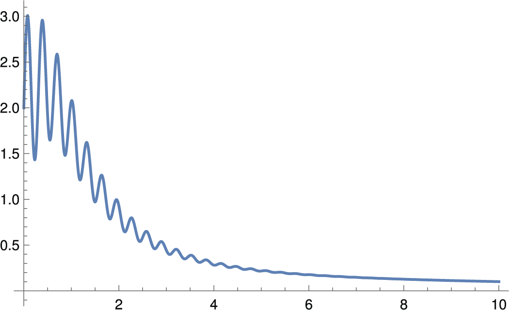
Example 4.4 (An example of an ‘oscillating’ but positive sine transform).
The sine transform of
 $$ \begin{align*} f(t):\!&= (1 + t) e^{-t} + \frac{2 t}{1 + t^2} + \frac{80 t}{(1 + (20 - t)^2) (1 + (20 + t)^2)} \\ &= (1 + t) e^{-t} + \frac{2 t}{1 + t^2} + \frac{1}{2} \bigg[\frac{1}{1 + (20 - t)^2} - \frac{1}{ 1 + (20 + t)^2)}\bigg] \end{align*} $$
can be evaluated directly and is given, apart from the normalisation constant, by
 $$ \begin{align*} g(\omega) = \frac{\omega}{1 + \omega^2} + \frac{2 \omega}{(1 + \omega^2)^2} + e^{-\omega} (2 + \sin(20 \, \omega)). \end{align*} $$
A plot of
 $g(\omega )$
is shown in Figure 1.
An ‘oscillating’ (not ‘oscillatory’) sine transform.

Since
 $f(0) = 1$
, Theorem 2.1 guarantees that the sine transform of
 $f(t)$
is indeed positive, at least for
 $$ \begin{align*} \omega> \int_0^{+\infty} |f"(t)| \, dt \approx 5.739. \end{align*} $$
These calculations were made by Mathematica.
Supplementary material
The supplementary material for this article can be found at https://doi.org/10.1017/S0004972725100403.
Acknowledgement
This work was carried out in the framework of the GNFM of the Italian INdAM.