2 Governing equations

The flow ( $\boldsymbol{u},p$ ) is governed by the incompressible Navier–Stokes equations expressed in non-dimensional form as:

(2.1) $$\begin{eqnarray}\displaystyle & \displaystyle \unicode[STIX]{x1D735}\boldsymbol{\cdot }\boldsymbol{u}=0, & \displaystyle\end{eqnarray}$$

(2.2) $$\begin{eqnarray}\displaystyle & \displaystyle \frac{\unicode[STIX]{x2202}\boldsymbol{u}}{\unicode[STIX]{x2202}t}+(\boldsymbol{u}\boldsymbol{\cdot }\unicode[STIX]{x1D735})\boldsymbol{u}=-\unicode[STIX]{x1D735}p+\frac{1}{Re}\unicode[STIX]{x1D6FB}^{2}\boldsymbol{u}. & \displaystyle\end{eqnarray}$$

Here, $\boldsymbol{u}$ , $p$ and $Re$ denote velocity, pressure and Reynolds number, respectively. The physical length and velocity scales have been non-dimensionalized using the chord length ( $c$ ) and free-stream speed ( $U_{\infty }$ ), respectively. The equation system (2.1)–(2.2) is accompanied by initial and boundary conditions. We adopt a perturbative approach wherein the flow is decomposed into base flow and disturbance quantities:

(2.3a,b ) $$\begin{eqnarray}\boldsymbol{u}=\boldsymbol{U}+\boldsymbol{u}^{\prime },\quad p=P+p^{\prime }.\end{eqnarray}$$

The base flow ( $\boldsymbol{U},P$ ) is the steady solution of equation system (2.1)–(2.2). On substituting (2.3) in equation system (2.1)–(2.2) and subtracting from it the equation for base flow, we get the following equation system that governs the evolution of the perturbation

(2.4) $$\begin{eqnarray}\displaystyle & \displaystyle \unicode[STIX]{x1D735}\boldsymbol{\cdot }\boldsymbol{u}^{\prime }=0, & \displaystyle\end{eqnarray}$$

(2.5) $$\begin{eqnarray}\displaystyle & \displaystyle \frac{\unicode[STIX]{x2202}\boldsymbol{u}^{\prime }}{\unicode[STIX]{x2202}t}+(\boldsymbol{U}\boldsymbol{\cdot }\unicode[STIX]{x1D735})\boldsymbol{u}^{\prime }+(\boldsymbol{u}^{\prime }\boldsymbol{\cdot }\unicode[STIX]{x1D735})\boldsymbol{U}+(\boldsymbol{u}^{\prime }\boldsymbol{\cdot }\unicode[STIX]{x1D735})\boldsymbol{u}^{\prime }=-\unicode[STIX]{x1D735}p^{\prime }+\frac{1}{Re}\unicode[STIX]{x1D6FB}^{2}\boldsymbol{u}^{\prime }. & \displaystyle\end{eqnarray}$$

Equation system (2.4)–(2.5) is accompanied by an initial condition for the perturbation and homogeneous boundary conditions. For infinitesimal perturbation analysis, the nonlinear term in the equation system (2.4)–(2.5) is dropped. In this situation, the perturbation evolution is governed by the linearized disturbance equations

(2.6) $$\begin{eqnarray}\displaystyle & \displaystyle \unicode[STIX]{x1D735}\boldsymbol{\cdot }\boldsymbol{u}^{\prime }=0, & \displaystyle\end{eqnarray}$$

(2.7) $$\begin{eqnarray}\displaystyle & \displaystyle \frac{\unicode[STIX]{x2202}\boldsymbol{u}^{\prime }}{\unicode[STIX]{x2202}t}+(\boldsymbol{U}\boldsymbol{\cdot }\unicode[STIX]{x1D735})\boldsymbol{u}^{\prime }+(\boldsymbol{u}^{\prime }\boldsymbol{\cdot }\unicode[STIX]{x1D735})\boldsymbol{U}=-\unicode[STIX]{x1D735}p^{\prime }+\frac{1}{Re}\unicode[STIX]{x1D6FB}^{2}\boldsymbol{u}^{\prime }. & \displaystyle\end{eqnarray}$$

3 Optimization

We seek an initial disturbance to the base flow that would maximize the gain of perturbation kinetic energy over a given time horizon $T$ . The kinetic energy of the perturbation at any time instant is defined as

(3.1) $$\begin{eqnarray}E(t)=\int _{\unicode[STIX]{x1D6FA}}\boldsymbol{u}^{\prime }(t)\boldsymbol{\cdot }\boldsymbol{u}^{\prime }(t)\,\text{d}\unicode[STIX]{x1D6FA},\end{eqnarray}$$

where the integration is carried out over the full computational domain ( $\unicode[STIX]{x1D6FA}$ ). Owing to the length and velocity scales used for non-dimensionalization, perturbation energy scales as $U_{\infty }^{2}c^{3}$ . The energy gain ( $G$ ) associated with a given initial perturbation and $T$ is given by

(3.2) $$\begin{eqnarray}G=\frac{E(T)}{E(0)}.\end{eqnarray}$$

Optimization is carried out in the linear framework where the perturbation evolution is governed by the equation system (2.6)–(2.7). The method of Lagrange multipliers is used for the computation of linear optimal perturbation/gain. This approach is similar to that described/used in Farrell (Reference Farrell1988), Corbett & Bottaro (Reference Corbett and Bottaro2000), Zuccher et al. (Reference Zuccher, Bottaro and Luchini2006), Schmid (Reference Schmid2007), Cherubini et al. (Reference Cherubini, De Palma, Robinet and Bottaro2011), Cherubini & De Palma (Reference Cherubini and De Palma2013), Schmid & Brandt (Reference Schmid and Brandt2014) and Kerswell (Reference Kerswell2018). Full details of the method were presented in our earlier article (Navrose et al. Reference Navrose, Brion, Jacquin and Robinet2018). We briefly describe it here. A Lagrangian functional ( ${\mathcal{L}}$ ) is formed with $G$ as the objective function and linearized disturbance equation system (2.6)–(2.7) as the constraint. The latter introduces adjoint variables in the Lagrangian formulation. For the optimal initial condition, the gradient of ${\mathcal{L}}$ vanishes. Setting to zero the variation of ${\mathcal{L}}$ with respect to its arguments gives the (i) direct equation (2.6)–(2.7), (ii) adjoint equation, (iii) compatibility condition between direct and adjoint variables at $t=T$ and (iv) optimality condition at $t=0$ . An iterative procedure is employed to find the optimal initial perturbation starting from a random perturbation field. In the first step of an iteration loop, the direct equation is solved from $t=0$ to $T$ . The adjoint equation is initialized using the compatibility condition and is then solved backwards in time from $t=T$ to 0. Finally, the optimality condition is used to update the initial condition for the direct equation. The direct–adjoint iterative procedure is carried on until adequate convergence is achieved.

4 Problem set-up, boundary conditions and spectral mesh

The set-up consists of a rectangular wing placed in a cuboidal domain with uniform velocity at the inlet boundary. The origin of the Cartesian coordinate system lies on the mid-plane of the wing and at the leading edge. The mid-plane coincides with the plane $y=0$ . The $x$ -axis of the coordinate system is along the direction of the incoming flow (also referred to as the streamwise direction). The $y$ - and $z$ -axes are along the spanwise and vertical directions, respectively. The streamwise length of the computational domain is $64c$ : $4c$ upstream and $60c$ downstream from the leading edge. In the spanwise direction, the side boundaries have been placed at a distance of $8c$ from the respective wing tips. The vertical position of the wing is such that its leading edge is located at a distance of $10c$ from the top and bottom boundaries. Two cross-sections of the wing have been considered: a flat plate with uniform thickness of $0.02c$ and a NACA0012 airfoil. The angle of attack of the wing with respect to the incoming flow is denoted by $\unicode[STIX]{x1D6FC}$ . Aspect ratio ( $AR$ ) of the rectangular wing is defined as the ratio between the wing span and chord length. Owing to the symmetry of the set-up about the mid-plane, computations have been carried out for a half-domain with the symmetry condition imposed on the mid-plane. We would like to note that the symmetry condition restricts optimization to perturbations that are symmetric about the mid-plane of the wing. A general perturbation to the base flow can be written as a linear combination of symmetric and anti-symmetric perturbations. It can be shown that within the linear framework, symmetric and anti-symmetric perturbations evolve independently of each other. In his seminal work, Crow (Reference Crow1970) found that the fastest growing instability in a counter-rotating vortex system is symmetric about the mid-plane. Since the major motivation for the present work was to identify a perturbation that can hasten the onset of the so-called Crow instability, which in turn, is expected to expedite the decay of tip vortices, using a symmetry condition on the mid-plane seemed a reasonable approach. An alternate approach to compute the symmetric (anti-symmetric) optimal perturbation is to carry out a computation in the full domain and use symmetric (anti-symmetric) perturbation as the initial guess for optimization. This approach would require much larger computational resources than a half-domain computation.

The rest of the boundary conditions are as follows. Free-stream values for the velocity are assigned at the inflow boundary. At the top, bottom, outflow and side boundaries (opposite to the symmetry plane) the stress vector is set to zero. No-slip condition is specified on the surface of the wing. NEK5000 (Fischer, Lottes & Kerkemeier Reference Fischer, Lottes and Kerkemeier2008), an open source spectral element solver, is used for the computations. The computational domain is divided into many spectral elements. Each spectral element is further discretized using Gauss–Lobato–Legendre (GLL) points. The spatial resolution of the domain is varied by changing the number of GLL points within each element. The number of grid points (including GLL decomposition) for the computation ranges from ${\sim}10$ to ${\sim}130$ million. Such spatial resolution is required to capture the flow accurately near the wing as well as its wake. Figure 1(a) shows the full sectional view of a spectral mesh in the $x{-}z$ plane. Figures 1(b) and 1(c) show a zoom-in view of the mesh near the flat plate and NACA0012 wing, respectively. The computations have been carried out in parallel utilizing 948–4096 cores. In general, for computing the flow up to 80 time units, around 40 000 CPU hours are spent (per case). Due to the constraints of computational resources, we have limited the time horizon for optimization study to $T\leqslant 15$ . It is shown later in the paper that although the value of optimal gain increases with $T$ , the general shape of the optimal perturbation remains nearly the same for $T\geqslant 5$ . Detailed mesh convergence tests have been performed to establish the adequacy of the mesh employed for the computations. The results for mesh convergence are presented later in the paper (§§ 6 and 8) along with the main results.

Figure 1.

Flow past a finite span wing: (a) sectional view ( $x{-}z$ plane) of a spectral mesh used for computations, (b) and (c) zoom-in view of the mesh ( $x{-}z$ plane) near the flat plate and NACA0012 wing, respectively.

5 Base flow description

Figure 2.

$Re=1000$ flow past a flat plate wing with $AR=6$ and $\unicode[STIX]{x1D6FC}=5^{\circ }$ : isosurface of total vorticity ( $|\unicode[STIX]{x1D714}|=0.1$ ). The direction of the incoming flow is along the $x$ -axis and is shown using a thick arrow. For the purpose of illustration, the isosurface has been shown for the full wing by reflecting the flow about the mid-plane. In the insets, spanwise ( $\unicode[STIX]{x1D714}_{y}=\pm 0.1$ ) and streamwise ( $\unicode[STIX]{x1D714}_{x}=0.1$ ) vorticity in the $y{-}z$ plane at distances of $5c$ , $10c$ , $25c$ , $35c$ , $45c$ and $55c$ from the leading edge of the wing are shown. The left part of each inset shows the spanwise vorticity, and the right part shows the streamwise vorticity. The tail of each arrow (with broken line) marks the streamwise location of the station and head points to the corresponding vorticity field.

The base flow for carrying out optimization is the fully developed flow past the finite wing. Figure 2 shows the isosurface of total vorticity for the $Re=1000$ flow. For illustration, the isosurface has been reflected about the symmetry plane so that the full wing span can be shown. The streamwise and spanwise components of vorticity at different streamwise locations are shown as insets in figure 2. Unless stated otherwise, results have been presented for a flat plate wing with $AR=6$ and $\unicode[STIX]{x1D6FC}=5^{\circ }$ . For $Re=1000$ , the fully developed flow in the computational domain is steady. Just downstream of the wing, the flow has a strong spanwise vorticity resulting from the no-slip condition imposed on the wing surface. In addition, a layer of streamwise vorticity exists in the near wake as well. The latter is attributed to finiteness of the lifting surface that allows the flow to go around the tip. The strength of the streamwise vorticity layer is largest near the tip of the wing and decreases to zero at the symmetry plane. The streamwise vorticity layer rolls up in the wake to form tip vortex. The roll-up occurs for a distance of approximately $15c$ from the leading edge. Beyond the roll-up distance, the wake can be divided into two parts based on the distribution of vorticity and streamwise velocity. The two parts are indicated in figure 2. One part corresponds to the tip vortex. This part is dominated by the streamwise component of vorticity and has a nearly axisymmetric deficit of streamwise velocity. The other part of the wake contains primarily spanwise vorticity. The streamwise velocity deficit in the second part of the wake is similar to that for the two-dimensional flow past a flat plate. Following Edstrand et al. (Reference Edstrand, Davis, Schmid, Taira and Cattafesta2016, Reference Edstrand, Schmid, Taira and Cattafesta2018), we refer to the second part of the wake as the trailing edge wake. The downwash induced by the wing and tip vortex separates the two parts of the wake. The separation increases with increase in downstream distance from the wing.

Figure 3.

Flow past a flat plate wing with $AR=6$ and $\unicode[STIX]{x1D6FC}=5^{\circ }$ : variation of (a) vertical and, (b) spanwise position of the centre of the tip vortex with downstream distance from the leading edge for various $Re$ .

Next, we present the downstream evolution of tip-vortex characteristics. Figure 3 shows the vertical and spanwise positions of the vortex centre at different downstream locations in the wake. The vortex centre, for a given streamwise location, is defined as the position of maximum streamwise vorticity in the corresponding $y{-}z$ plane. This position nearly coincides with the location of minimum pressure and the barycentre of the streamwise vorticity on the same plane. It is observed that, with respect to the streamwise direction, the tip vortex is inclined in the vertical direction. This is attributed to the velocity imposed by the counter-rotating vortex present on the other side of the symmetry plane. Beyond the vortex roll-up distance ( $x\gtrsim 15c$ ), the vertical inclination of the tip vortex is nearly constant. Using a least squares linear fit of the data points between $x=20c$ and $50c$ in figure 3(a) for $Re=1000$ , we calculate the inclination angle in the $x{-}z$ plane as ${\sim}0.42^{\circ }$ . The tip vortex is also inclined in the spanwise direction; the inclination is relatively large near the trailing edge of the wing and decreases with downstream distance. The spanwise inclination of the tip vortex occurs because the barycentre of the axial vorticity layer formed over the wing surface is not at the wing tip but slightly in towards the wing root. The location of the barycentre moves towards the wing root during the roll-up process (Krasny Reference Krasny1987). Least squares linear fitting of data points between $x=30c$ and $50c$ for $Re=1000$ in figure 3(b) yields a spanwise inclination of the vortex axis of ${\sim}0.17^{\circ }$ . The relatively low value of the two inclination angles makes it reasonable to assume that the axis of the tip vortex is along the streamwise direction. This assumption allows identification of the tip vortex using the isosurface of streamwise vorticity.

A rough estimate of the vertical inclination of the tip vortex can also be made from the value of circulation ( $\unicode[STIX]{x1D6E4}$ ) of the tip vortex and the spanwise separation between it and its counter-rotating image. For a two-dimensional (2-D) counter-rotating vortex pair with strength $\unicode[STIX]{x1D6E4}$ and vortex separation distance $b$ , the velocity of the vertical descent of the vortex pair estimated using a point vortex model is $v_{d}=\unicode[STIX]{x1D6E4}/(2\unicode[STIX]{x03C0}b)$ . In free-stream conditions, the 2-D vortex pair will get convected in the streamwise direction as it descends vertically. The angle of vertical inclination between the original streamwise position of the vortex and that at a later time instant is $\tan ^{-1}(v_{d}/U_{\infty })$ . For the flow computed at $Re=1000$ (figure 2), the vertical inclination calculated using the value of circulation and vortex separation distance at $x=20c$ is ${\sim}0.33^{\circ }$ . The angle so obtained is similar to that calculated earlier via linear fitting of the data points of figure 3(a): $0.42^{\circ }$ .

Figure 4.

Flow past a flat plate wing with $AR=6$ and $\unicode[STIX]{x1D6FC}=5^{\circ }$ : variation of (a) square of the tip-vortex radius and, (b) strength of the tip vortex with downstream distance from the leading edge for various $Re$ .

Figure 4(a) shows the variation of the square of the vortex dispersion radius ( $a$ ) with streamwise distance from the leading edge. It is obtained using the relation

(5.1) $$\begin{eqnarray}a^{2}=\frac{\displaystyle \int _{\unicode[STIX]{x1D734}}r^{2}\unicode[STIX]{x1D714}\,\text{d}\unicode[STIX]{x1D734}}{\unicode[STIX]{x1D6E4}},\end{eqnarray}$$

where $r$ is the distance measured from the vortex centre, $\unicode[STIX]{x1D714}$ is the axial vorticity and $\unicode[STIX]{x1D6E4}$ is the circulation associated with the vortex at the corresponding streamwise location. The value of circulation is given by

(5.2) $$\begin{eqnarray}\unicode[STIX]{x1D6E4}=\int _{\unicode[STIX]{x1D734}}\unicode[STIX]{x1D714}\,\text{d}\unicode[STIX]{x1D734}.\end{eqnarray}$$

The domain of integration in (5.1)–(5.2) is taken to be the region in the $y{-}z$ plane where the value of $\unicode[STIX]{x1D714}$ is greater than 5 % of the maximum axial vorticity. It is observed that for a given $Re$ , $a^{2}$ increases almost linearly with streamwise distance from the wing. Earlier works have shown that the vortex dispersion radius of an isolated 2-D Lamb–Oseen ( $a_{LO}$ ) increases with time due to viscous dissipation, and that $\unicode[STIX]{x0394}a_{LO}^{2}$ for a given Reynolds number is directly proportional to the time interval (Saffman Reference Saffman1992). Here, the $\unicode[STIX]{x1D6E5}$ symbol represents change in the corresponding quantity. Lamb–Oseen vortex is a popular 2-D vortex model used in the study of the dynamics of vortex systems. If the Lamb–Oseen vortex convects in the streamwise direction under free-stream conditions, then $a_{LO}^{2}$ will increase in proportion to the streamwise distance, and hence, its variation will be similar to that shown in figure 4(a). This suggests that the downstream increase in the dispersion radius of the tip vortex obtained via the present numerical simulation can be attributed to viscous dissipation. With an increase in $Re$ , the effect of viscosity decreases. Consequently, the slope of the $a^{2}$ curve decreases with $Re$ . Figure 4(b) shows the variation of circulation with streamwise distance for various $Re$ . The circulation remains nearly constant with distance for a given $Re$ . This is in line with the prediction made from inviscid analysis of the flow past a finite wing (Saffman Reference Saffman1992). With an increase in $Re$ , the strength of the tip vortex (measured by circulation) increases. For $Re=3000$ , the trailing edge wake becomes unsteady with significant axial vorticity contained in it. Hence, while carrying out integration of (5.2), some region of the trailing edge wake is also included in the domain of integration. This results in an increase in the value of circulation for $Re=3000$ as shown in figure 4(b).

Figure 5.

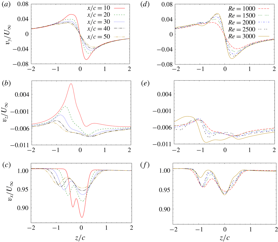
Flow past a flat plate wing with $AR=6$ and $\unicode[STIX]{x1D6FC}=5^{\circ }$ : variation of (a,d) spanwise, (b,e) vertical and (c,f) streamwise component of velocity at a given streamwise location along a line parallel to the $z$ -axis and passing through the vortex centre. (a–c) Shows results for $Re=1000$ and different streamwise locations. (d–f) Shows results for $x=40c$ and different $Re$ .

For further characterization of the tip vortex, we extract, at a given streamwise location, the velocity along a line that is parallel to the $z$ -axis and passes through the respective vortex centre. We denote such a line by $l_{vc}$ (where the subscript $vc$ means vortex centre). The reference point for defining the position along $l_{vc}$ is the vortex centre. Figure 5(a) shows the variation of the spanwise component of velocity ( $v_{y}$ ) along $l_{vc}$ for $Re=1000$ at different streamwise locations. Since the vortex axis is nearly aligned in the streamwise direction, the distribution of spanwise velocity along $l_{vc}$ gives an approximate distribution of the azimuthal velocity of the tip vortex; $v_{y}$ is nearly zero at the vortex centre for all streamwise locations. For positive $z$ , the direction of spanwise velocity is towards the symmetry plane. For negative $z$ , spanwise velocity is directed towards the wing tip. In the vicinity of the vortex centre, the variation of $v_{y}$ along $l_{vc}$ is linear. Beyond the linear regime, the magnitude of $v_{y}$ ( $|v_{y}|$ ) reaches a peak value on either side of the vortex centre, and then decreases with an increase in distance from the vortex centre. The distance between the two peaks gives an estimate of the size of the vortex core. It is observed that the diameter of the vortex core increases downstream. Concomitantly, the peak value of streamwise vorticity within the vortex core decreases (in accordance with Helmholtz’s first theorem: circulation of a vortex tube is constant along its length). At relatively large distance from the vortex core, $|v_{y}|$ decreases almost inversely with distance from the vortex centre ( $|v_{y}|\sim 1/z$ ). In this flow region, the tip vortex can be assumed to be irrotational. Figure 5(b) shows the variation of the vertical component of velocity ( $v_{z}$ ) along $l_{vc}$ . The prominent negative value of $v_{z}$ is in line with the downward motion of the tip vortex under the effect of its counter-rotating pair. Since $v_{z}$ varies within the vortex core, the tip vortex experiences stretching in the vertical direction. As a result, the tip vortex takes a slightly elliptical shape. The streamwise velocity ( $v_{x}$ ) variation along $l_{vc}$ (figure 5 c) shows two peaks: one is associated with the velocity deficit within the vortex, and the other corresponds to the deficit in the trailing edge wake. The distance between the two peaks increases downstream. At sufficiently large distance from the wing, the streamwise velocity deficit within the vortex core becomes close to axisymmetric.

Figure 6.

Flow past a flat plate wing with $AR=6$ and $\unicode[STIX]{x1D6FC}=5^{\circ }$ : isosurface of total vorticity for (a) $Re=2500$ , (b) $Re=3000$ and (c) $Re=5000$ . For illustration, the isosurfaces are shown for the full wing by reflecting the flow about the mid-plane. The location of the wing is shown in blue colour at the top left corner of each frame.

With an increase in $Re$ , the flow remains steady up to $Re=2500$ (figure 6 a). The evolution of the vortex centre with downstream distance (figure 3 a,b), and velocity distribution within the tip vortex (figure 5 d–f) is found to be similar for $1000\leqslant Re\leqslant 2500$ . For $Re=3000$ , the flow becomes unsteady (figure 6 b) and a Kármán vortex street is observed in the trailing edge wake. For $Re=5000$ , the trailing edge wake seems to transition to a turbulent state (figure 6 c). The tip vortex, however, retains its laminar behaviour at $Re=5000$ .

6 Optimal gain and perturbation

Figure 7.

$Re=1000$ flow past a flat plate wing with $\unicode[STIX]{x1D6FC}=5^{\circ }$ and $AR=6$ : (a) variation of linear optimal gain with time horizon and (b) isosurface of spanwise vorticity ( $\pm 0.2$ ) for $T=10$ linear optimal perturbation. The wing root lies on the plane of symmetry of the geometrical set-up.

Figure 8.

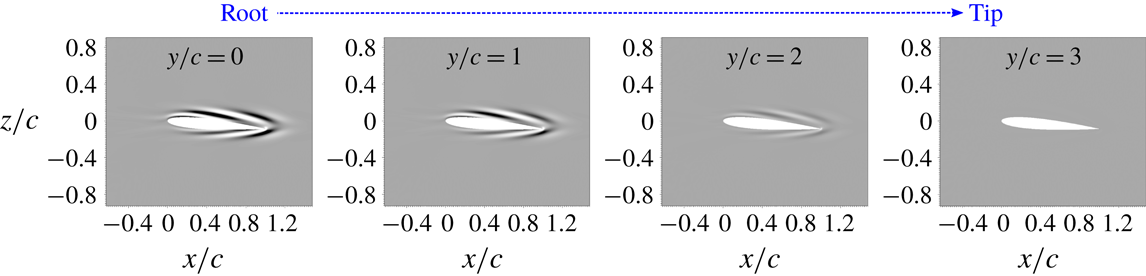
$Re=1000$ flow past a flat plate wing with $\unicode[STIX]{x1D6FC}=5^{\circ }$ and $AR=6$ : sectional view of (a) spanwise vorticity ( $\pm 0.2$ ) and (b) streamwise vorticity ( $\pm 0.01$ ) for $T=10$ linear optimal perturbation in different spanwise planes (from root to the wing-tip).

Table 1.

Effect of polynomial order of spectral element on the value of linear optimal gain for various time horizons.

Optimization has been carried out in the flow regime where the fully developed flow is steady. Figure 7(a) shows the variation of linear optimal gain ( $G$ ) with time horizon for $Re=1000$ , $AR=6$ , $\unicode[STIX]{x1D6FC}=5^{\circ }$ and a flat plate wing. The values of gain for different $T$ reported in figure 7(a) are obtained after rigorous mesh convergence tests. The results of the mesh convergence study are summarized in table 1. The order of the polynomial (related to the number of GLL points in a spectral element) required to adequately capture the evolution of the perturbation depends on the time horizon over which optimization has been carried out. For example, for $T=5$ , $p=6$ is sufficient, while for $T=15$ , at least $p=12$ is needed for adequate resolution. This is because of the nature of the evolution of the optimal perturbation, and the use of a non-uniform mesh in capturing it (discussed in detail in § 8). It is observed that $G$ increases monotonically with $T$ up to the largest time horizon that has been investigated. The shape of the linear optimal perturbation, on the other hand, does not change significantly with $T$ . Optimal perturbation is located near the wing surface (figure 7 b) and is dominated by the spanwise component of vorticity. All three components of vorticity are arranged as spanwise parallel sheets of alternate sign that are inclined to the surface of the wing. The strength of the spanwise vorticity sheets is largest at the root of the wing and decreases along the wing span to become negligible at the tip (figure 8 a). The streamwise and vertical components of vorticity are relatively weaker than the spanwise component. Both the components are absent near the root and the tip of the wing (figure 8 b).

The shape of the optimal perturbation shown in the $x{-}z$ plane (figure 8 b) resembles that for the 2-D flow past a flat plate (Akervik et al. Reference Åkervik, Ehrenstein, Gallaire and Henningson2008). In the 2-D set-up, the transient growth of energy occurs via two concurrent mechanisms: downstream motion of the perturbation wavepacket, and increase in the energy of the wavepacket via the Orr mechanism (Orr Reference Orr1907). Since the optimal perturbation is located away from the wing tip, the initial evolution of the optimal perturbation is not affected by the flow modification arising because of the wing tip. The initial growth of energy, therefore, occurs via the 2-D Orr mechanism (in the $x{-}z$ plane). At later stages, due to the strong three-dimensionality of the flow resulting from the roll-up of the axial vorticity layer, the perturbation gets transferred to the tip-vortex region (discussed in detail in §§ 7 and 8), and the evolution deviates from the 2-D evolution via the Orr mechanism.

The location of the optimal perturbation is quite interesting as it brings focus to the role of the near wake region in amplifying the disturbance in a trailing vortex system. Within the streamwise distance where the optimal perturbation is located, the tip vortex has either not formed, or is in a nascent stage of its formation. As shown in the next section, the perturbation introduced near the wing surface gets transferred in the tip-vortex region during its evolution, and results in vortex deformation several chord lengths downstream of the wing. Vortex deformation, in turn, may expedite the decay of tip vortices via various mechanisms, for example, earlier onset of the Crow instability (Crow Reference Crow1970) in the far wake.

Another feature of the optimal perturbation brought out by figures 7(b) and 8 is that the optimal perturbation can introduce significant modification to the flow around the wing. This is reflected in the difference in the values of the aerodynamic coefficients without and with optimal perturbation. We take the example of $T=10$ linear optimal perturbation with $E(0)=10^{-4}$ . Since energy is non-dimensionalized using $U_{\infty }^{2}c^{3}$ , $E(0)=10^{-4}$ represents a relatively small fraction of the free-stream flow energy. For unperturbed flow, the values of the lift ( $C_{L}$ ) and drag coefficients ( $C_{D}$ ) are 0.96 and 0.36, respectively. If the optimal perturbation is added to the base flow, the instantaneous values of $C_{L}$ and $C_{D}$ change to $-0.005$ and 0.22, respectively. As the perturbation evolves with time, the values of the aerodynamic coefficients relax toward those of the unperturbed flow. Thus, when employing the optimal perturbation for control of an aircraft trailing vortex system, the instantaneous change in the value of the aerodynamic coefficients due to the addition of the optimal perturbation can be an important consideration. Strong initial perturbation (large $E(0)$ ) can introduce large disturbance to the wake but might result in significant loss of instantaneous lift. Weak perturbation (small $E(0)$ ) may not affect aerodynamic coefficients significantly, but it might turn out to be ineffective for controlling the wake.

Table 2.

Effect of flow and geometry parameters on the value of linear optimal gain. Aerodynamic coefficients are for the corresponding base flow that is used for optimization.

Parametric exploration is carried out over $Re$ , aspect ratio ( $AR$ ), angle of attack ( $\unicode[STIX]{x1D6FC}$ ) and shape of the airfoil, to study their effects on the linear optimal gain and perturbation. The time horizon is fixed as $T=10$ . We select $Re=1000$ , $AR=6$ , $\unicode[STIX]{x1D6FC}=5^{\circ }$ and the flat plate wing as the base case about which the parameters are varied one at a time. The parametric study brings out several important features of the optimal perturbation and its results are summarized in table 2. First, optimal gain increases exponentially with increase in $Re$ . Using least-squares curve fitting, this dependence is found as $G\sim \text{e}^{(0.0062Re)}$ . Second, with increase in $AR$ , the value of optimal gain increases. The fraction of the wing surface over which the flow is noticeably affected by finiteness of the wing is expected to decrease with an increase in $AR$ . The parametric variation of $G$ with $AR$ suggests that the lower is the fraction, the higher is the amplification of the initial perturbation energy. Optimal gain, therefore, would be largest for infinite span (nominally two-dimensional) wing. Our computations show that 2-D optimal gain is indeed higher than the gain obtained for finite wing. Third, $G$ increases with increase in $\unicode[STIX]{x1D6FC}$ . Finally, modifying the wing cross-section from a flat plate to the NACA0012 airfoil has a severe effect on optimal gain: the value for NACA0012 is an order higher than the flat plate. The change in $G$ may be attributed to the difference in the base flow for the two wing geometries. The difference is evident in the value of aerodynamic coefficients associated with the two base flows (table 2). Since the perturbation derives energy from the base flow, modification to the base flow will have an effect on the amplification of initial energy.

Figure 9.

$Re=1000$ flow past NACA0012 rectangular wing with $\unicode[STIX]{x1D6FC}=5^{\circ }$ and $AR=6$ : spanwise vorticity associated with $T=10$ linear optimal perturbation at various spanwise locations (from the root to the wing tip). The wing root lies on the plane of symmetry of the geometrical set-up.

Despite linear optimal gain being sensitive to the change in the parameters, the general shape of the linear optimal perturbation is similar over the entire parameter space that has been explored (for example, compare figures 9 and 8 a). This result is desirable from the perspective of flow control as the optimal perturbation computed for one set of parameters can be utilized for controlling flow over a wide parameter space.

7 Nonlinear evolution of linear optimal perturbation

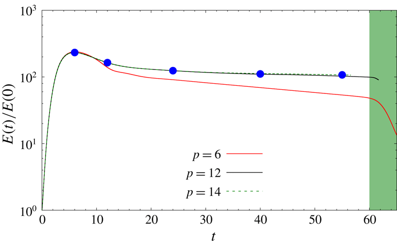
Direct time integration of the equations governing the nonlinear evolution of perturbation (2.4)–(2.5) is carried out using the $T=10$ linear optimal perturbation as the initial condition. Computations are carried out for $Re=1000$ , $AR=6$ , $\unicode[STIX]{x1D6FC}=5^{\circ }$ and the flat plate wing. The initial energy of the perturbation is set to $E(0)=10^{-4}$ . Figure 10 shows the variation of energy gain with time obtained using spectral elements of polynomial orders $p=6$ , 12 and 14. Energy gain is nearly insensitive to the spatial resolution of the mesh beyond $p=12$ . In addition, the evolution of of the shape of the perturbation is found to be nearly the same for $p\geqslant 12$ . We, therefore, present results obtained using $p=12$ . Figure 11(a,c,e,g,i) shows the spanwise component of perturbation vorticity on the symmetry plane at various time instants during the flow evolution. The perturbation vorticity at $t=0$ is shown earlier in the paper, in figure 8(a). It is observed that the perturbation evolves as a downstream travelling wavepacket. The speed of the wavepacket is nearly constant and is close to the free-stream speed. This is evident from the approximate matching of the streamwise location of the perturbation wavepacket and corresponding normalized time in figure 11(a,c,e,g,i). The energy of the wavepacket increases with time initially, reaches a peak value at $t\sim 5$ and then starts to decrease (figure 10). The value of the energy gain at $t=10$ is an order lower than linear energy gain corresponding to $T=10$ optimal perturbation (figure 7 a). For $25<t<60$ , the rate of energy decrement is reduced significantly as compared to that at smaller time. In this time interval, energy of the perturbation wavepacket appears to be nearly constant. We refer to the time interval as a quasi-steady interval. For $t\sim 59$ , the wavepacket reaches the outflow boundary, and later gets convected out of the computational domain. The energy gain, therefore, decreases rapidly beyond $t\sim 59$ .

Figure 10.

$Re=1000$ flow past a flat plate wing with $\unicode[STIX]{x1D6FC}=5$ and $AR=6$ : variation of energy gain with time for nonlinear evolution of $T=10$ linear optimal perturbation. Initial energy of the perturbation is $E(0)=10^{-4}$ . Energy curves obtained using different polynomial orders ( $p$ ) for the spectral element are shown in different colours. The blue coloured filled circles correspond to the time instants at which the flow is shown in figure 11. In the shaded time interval the perturbation is either leaving or has moved out of the computational domain.

Figure 11.

$Re=1000$ flow past a flat plate wing with $\unicode[STIX]{x1D6FC}=5$ and $AR=6$ : perturbation vorticity at various time instants obtained using $T=10$ linear optimal perturbation as initial condition for direct time integration of nonlinear equations (2.4)–(2.5). Each row corresponds to the flow at a time instant. (a,c,e,g,i) Shows spanwise vorticity ( $\pm 0.2$ ) on the symmetry plane ( $y=0$ ) and (b,d,f,h,j) shows the corresponding isosurface of streamwise vorticity ( $\pm 0.1$ ). The time instant is indicated on the top right corner of the frame that shows the spanwise vorticity. The position of the base flow tip vortex is indicated using a dotted outline in the last frame of right column.

Figure 12.

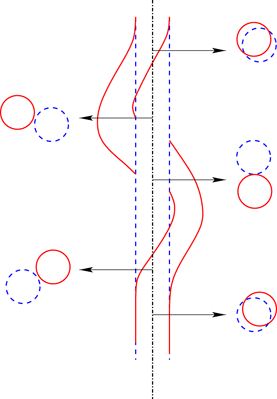
Flow past a finite $AR$ flat plate wing: schematic of the unperturbed (blue broken line) and perturbed tip vortex (red solid line) in the $x{-}y$ plane. The perturbation corresponds to the nonlinear wavepacket generated by $T=10$ linear optimal perturbation at $t=55$ (shown in figure 11). The unperturbed vortex axis is shown as the dashed-dotted line. Shown alongside on either side is the view of the unperturbed and perturbed vortices in the $x{-}z$ plane at different streamwise locations (shown via arrow) along the vortex axis.

Figure 13.

$Re=1000$ flow past a flat plate wing with $\unicode[STIX]{x1D6FC}=5$ and $AR=6$ : instantaneous signal of spanwise ( $v$ ) and transverse ( $w$ ) component of velocity along the axis of the tip vortex as the perturbation wavepacket travels downstream. (a) $t=10$ , (b) $t=20$ , (c) $t=30$ , (d) $t=40$ , (e) $t=50$ and (f) $t=60$ .

Figure 14.

(a) $Re=1000$ flow past a flat plate wing with $\unicode[STIX]{x1D6FC}=5$ and $AR=6$ : trajectory traced by the vortex centre in the $y{-}z$ plane at three streamwise locations as the perturbation wavepacket passes through the three locations. The initial perturbation is the $T=10$ linear optimal perturbation with $E(0)=10^{-4}$ . (b) Vortex position in the cross-flow plane at various time instants obtained via experiment by Roy & Leweke (Reference Roy and Leweke2008). The thick red line in (b) corresponds to the average motion of the vortex centre.

The existence of a quasi-steady interval in the evolution of the linear optimal perturbation brings out two important features of the flow past a finite wing: a perturbation generated near the wing surface can disturb the flow several chord lengths downstream of the wing, and, the downstream wavepacket is stronger than the initial perturbation near the wing surface. For example, for $E(0)=10^{-4}$ , the energy of the perturbation wavepacket in the quasi-steady interval is two orders of magnitude higher than the initial perturbation energy. Beyond the vortex roll-up distance ( $x\gtrsim 15c$ ), the wavepacket within the tip-vortex region is structured as two elongated strands of streamwise vorticity, one positive and the other negative, intertwined helically along the streamwise direction (figure 11 b,d,f,h,j). The structure is redolent of the $m=1$ bending mode that is associated with the deformation of an isolated vortex column (Fabre, Sipp & Jacquin Reference Fabre, Sipp and Jacquin2006). The effect of the bending mode is to displace the vortex column from its unperturbed location (Antkowiak & Brancher Reference Antkowiak and Brancher2004; Pradeep & Hussain Reference Pradeep and Hussain2006). Therefore, the perturbation wavepacket causes a shift in the position of the tip vortex beyond $x\sim 15c$ . A schematic of the unperturbed and perturbed tip vortices is shown in figure 12. To further analyse the deformation of the tip vortex as the perturbation wavepacket travels through it, we record the velocity along the centreline of the tip vortex at various time instants. The signal for the spanwise ( $v$ ) and vertical ( $w$ ) components of the velocity is shown in figure 13. The downstream movement of the perturbation wavepacket can be seen from the top to the bottom frame of the figure. Within the wavepacket, the two velocity signals have a phase difference of between $0^{\circ }$ and $180^{\circ }$ . 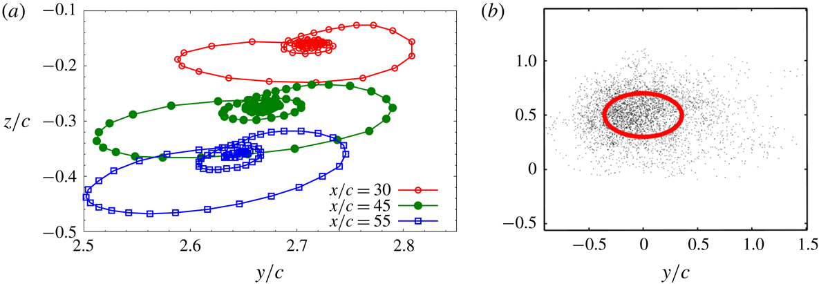Accordingly, as the wavepacket passes a given streamwise location, vortex centre traces elliptical trajectories in the $y{-}z$ plane. Figure 14(a) shows the vortex centre trajectory at three streamwise locations. The rotation of the axes of the ellipse suggests that the perturbation wavepacket within the tip vortex rotates about the axis of tip vortex.

Figure 15.

$Re=1000$ flow past a flat plate wing with $\unicode[STIX]{x1D6FC}=5$ and $AR=6$ : variation of energy gain with time for linearized simulation carried out using different polynomial orders of spectral elements. Initial condition for the simulation is $T=10$ linear optimal perturbation. In the shaded time interval the perturbation is either leaving or has moved out of the computational domain. For comparison, the energy gain curve obtained via the $p=12$ nonlinear simulation is also shown.

8 Comparison of linear and nonlinear evolution of perturbation

It is observed that the value of energy gain obtained via nonlinear simulation (figure 10) at $t=10$ is an order of magnitude lower than the value of $T=10$ linear optimal gain. Nonlinear terms, therefore, can have significant effect on the evolution of the linear optimal perturbation even with relatively low $E(0)$ . To further explore the effect of the nonlinear terms, direct time integration of the linearized disturbance equations (2.6)–(2.7) is carried out and the results are compared with those obtained via nonlinear simulation. Reynolds number, initial condition and geometrical parameters for the linearized computation are the same as in § 7. Similar to the nonlinear simulation, the perturbation evolves like a downstream travelling wavepacket in the linearized simulation. Figure 15 shows the variation of linear energy gain with time computed using different values of $p$ for the spectral element. As noted before, the linear energy gain reaches a higher peak value than the nonlinear energy gain. Two additional observations are made. First, the linear simulation requires a higher spatial resolution of the spectral mesh than the nonlinear simulation. Close to the wing, the density of spectral elements is relatively high. In this flow region, $p=6$ accurately captures the evolution of the linear optimal perturbation in both linear and nonlinear simulations. This is evident from overlapping of the energy gain curves for $p\geqslant 6$ at short times (figures 10 and 15). The density of spectral elements decreases downstream, and therefore, higher-order polynomial is needed for accurate resolution of the perturbation wavepacket as it travels downstream. For nonlinear simulation, $p=12$ maintains adequate spatial resolution up to the outflow boundary. On the other hand, for the linear simulation, $p=12$ is insufficient once the perturbation wavepacket has travelled beyond $x\sim 30c$ . The difference in the linear energy gain curve for $p=12$ and 14 beyond $t\sim 30$ in figure 15 shows the inadequacy of the $p=12$ linearized simulation. We could not carry out a computation for $p>14$ because of the constraint of computational resources and time. Hence, we cannot ascertain if even $p=14$ accurately captures the linearized evolution of perturbation wavepacket up to the outflow boundary. Second, saturation of the perturbation energy (quasi-steady interval) is not apparent in the linear energy gain curve. In the nonlinear simulation, the quasi-steady interval starts at approximately $t=25$ . On the other hand, for the linearized simulation, energy gain continues to decrease beyond $t=25$ . The aforementioned observations bring out the importance of nonlinear effects in the near wake dynamics of the wing and in maintaining the energy of perturbation within the vortex core up to large streamwise distances from the wing rather than decay as suggested by the linear simulation.

Figure 16.

$Re=1000$ flow past a flat plate wing with $\unicode[STIX]{x1D6FC}=5$ and $AR=6$ : spanwise vorticity in the $x{-}z$ and $x{-}y$ planes, and isosurface of streamwise vorticity for the perturbation wavepacket obtained via linear and nonlinear simulations at two similar time instants. The left column shows results from the linear simulation and the right column shows results from the nonlinear simulation. In (a) perturbation wavepacket is located in the near wake region ( $x\sim 5c$ ), and in (b) it is located beyond the vortex roll-up distance ( $x\sim 21c$ ).

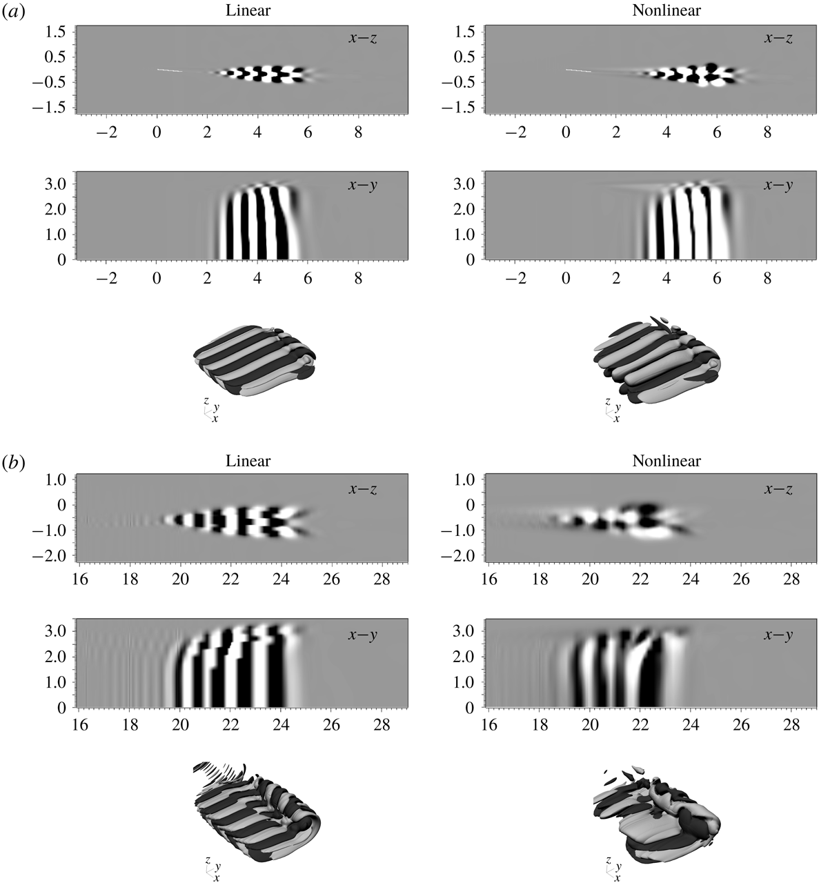
Figure 16 shows vorticity components for the linear and nonlinear perturbation wavepackets at two similar time instants: one corresponds to the situation when the wavepacket is relatively close to the wing, and the other when the wavepacket has travelled beyond the vortex roll-up distance. Close to the wing, the shape of the perturbation wavepacket obtained via the linear and nonlinear simulations is largely similar (figure 16 a). The vorticity components are arranged as spanwise rows of chevron-like pattern with alternate signs that extend from the trailing edge wake to the tip-vortex region. The chevron-like pattern is similar to that observed during the evolution of linear optimal perturbation in 2-D flow past a flat plate wherein the energy growth occurs by the Orr mechanism (Akervik et al. Reference Åkervik, Ehrenstein, Gallaire and Henningson2008). Beyond the vortex roll-up distance, the chevron-like pattern is maintained in the trailing edge wake for the linearized simulation (figure 16 b, left column). Within the tip-vortex region, the linearly evolved perturbation wavepacket appears as if the chevron pattern has been rolled-up. The sharp variation in vorticity isosurface might be attributed to inadequacy of the $p=14$ polynomial to capture the wavepacket at the corresponding streamwise location. In the nonlinear simulation, the chevron-like arrangement is not discernible in the trailing edge part of the wake (figure 16 b, right column). In the tip-vortex region, streamwise vorticity for the nonlinear perturbation wavepacket appears as two streamwise elongated strands that are wound helically around each other. The nonlinear wavepacket, as discussed earlier in § 7, results in displacement of the tip vortex. The linear wavepacket, despite having higher energy than the nonlinear wavepacket, causes no perceptible displacement of the tip vortex.

Figure 17.

$Re=1000$ flow past a flat plate wing with $\unicode[STIX]{x1D6FC}=5$ and $AR=6$ : variation of energy gain with time for the case where initially nonlinear terms are present in the disturbance equations and then later they are switched off. The initial disturbance corresponds to $T=10$ linear optimal perturbation with $E(0)=10^{-4}$ . The time instant when the switch-off occurs ( $t=20$ ) is shown on the energy gain curve by the blue dot. The part of the curve prior to the switch-off is shown by the solid line, and after switch-off is shown by the broken line. For comparison, the energy gain curve for the simulation where nonlinear terms are not switched off is shown using a solid line after $t=20$ .

The results presented in the preceding paragraphs show that within the vortex roll-up distance, the nonlinear term modifies the energy and shape of the perturbation wavepacket. Beyond the vortex roll-up distance, the general shape of the linear and nonlinear wavepackets does not change with time. To investigate the effect of nonlinear terms on the energy of the perturbation wavepacket beyond the vortex roll-up distance, we carry out direct time integration of the disturbance equations in two stages. In the first stage, using $T=10$ linear optimal perturbation ( $E(0)=10^{-4}$ ) as the initial condition, the perturbation is allowed to evolve nonlinearly up to $t=20$ . At $t=20$ , the nonlinear perturbation wavepacket has travelled beyond the vortex roll-up distance and is located at $x\sim 20c$ . In the second stage of the simulation, the nonlinear term is switched off, and the perturbation wavepacket evolves linearly beyond $t=20$ . Figure 17 shows the variation of energy gain with time for the two stages of the simulation: nonlinear stage (before switch-off) is shown using the solid line and the linear stage (after switch-off) is shown using the broken line. The time instant of switch-off is marked by the solid circle on the energy gain curve. It is observed that in the linear stage the energy gain decreases initially (inset of figure 17) and then increases monotonically with time until the perturbation wavepacket has reached the outflow boundary. The monotonic increase in energy gain is in agreement with recent results by Edstrand et al. (Reference Edstrand, Schmid, Taira and Cattafesta2018) on linear stability of the wake behind a finite wing for $Re=1000$ . By carrying out a local analysis of the wake at different streamwise locations, they showed that the wake is spatially unstable to downstream travelling perturbation waves. Therefore, the linear asymptotic analysis suggests that a general perturbation to the wake may grow downstream. We observe that in the linear stage of the simulation, the energy of the perturbation wavepacket indeed grows after an initial decrement. The initial dip in the energy gain (inset of figure 17) may be attributed to transient effects that are not accounted for in the asymptotic analysis. If nonlinear terms are kept switched on in the second stage of the simulation, energy gain does not increase after $t=20$ (solid line in figure 17). Since the value of $E(0)$ is set to $10^{-4}$ and the energy gain after transient effects is ${\sim}10^{-2}$ , we deduce that a perturbation wavepacket with energy ${\sim}\mathit{O}(10^{-2})$ is strong enough to deviate the flow evolution from that predicted by linear analysis. We would like to note that since the typical peak azimuthal velocity inside the tip vortex is an order lower than the free-stream speed, non-dimensional energy based on former will be two orders higher than that based on latter. Hence, a perturbation wavepacket with energy of the order of unity (based on peak azimuthal velocity of the tip vortex) will result in significant flow modification via nonlinear effects.

9 Vortex meandering

9.1 Steady base flow regime $(Re\leqslant 2500)$

Nonlinear simulation of linear optimal perturbation shows that the perturbation wavepacket causes movement of the vortex core. The motion occurs in such a way that the vortex centre traces elliptical trajectories. Once the perturbation wavepacket has passed a given streamwise location, the vortex centre at that location returns to its unperturbed position. In a situation where the linear optimal perturbation is injected periodically into the flow (as a method for flow control), it is expected that the vortex centre at all streamwise location would trace elliptical trajectories periodically. Furthermore, if the optimal perturbation is injected aperiodically, it will result in seemingly random motion of the vortex. The motion of the tip vortex, in this situation, will resemble the phenomenon of vortex meandering that has been observed in wind tunnel experiments of tip vortices (Roy & Leweke Reference Roy and Leweke2008). Figure 14(b), taken from Roy & Leweke (Reference Roy and Leweke2008), shows the ensemble of the positions of the vortex centre at different time instants for a fixed streamwise location. Atop the ensemble, the region where the vortex centre is located with a given probability is shown by the thick red line. The region is an ellipse that has similar orientation of its axes as that of the vortex motion induced by the linear optimal perturbation (see figure 14 a). Based on this observation, we propose, in addition to spatial instability (Edstrand et al. Reference Edstrand, Schmid, Taira and Cattafesta2018) and response to stochastic forcing (Fontane et al. Reference Fontane, Fabre and Brancher2008), another possible mechanism behind vortex meandering. That the perturbation generated near the wing surface gets amplified in the near wake region owing to transient effects, and is subsequently transferred to the tip-vortex region during the roll-up process. During these stages, nonlinear terms play a crucial role in shaping up the perturbation wavepacket. As the nonlinear wavepacket travels downstream, it causes a motion of the tip vortex that resembles meandering.

In the absence of an externally forced perturbation, the optimal perturbation can arise if the flow system is receptive to naturally occurring disturbances like free-stream sound waves or vortical structures. We make this conjecture based on the results of Fontane et al. (Reference Fontane, Fabre and Brancher2008) and Schrader, Brandt & Henningson (Reference Schrader, Brandt and Henningson2009). Fontane et al. (Reference Fontane, Fabre and Brancher2008) studied the response of a Lamb–Oseen vortex column to stochastic forcing. The motivation behind using stochastic forcing was to mimic uncontrolled (in space and time) ambient fluctuations like background turbulence. They found that optimal perturbations can be naturally activated by the background noise present in uncontrolled conditions. Schrader et al. (Reference Schrader, Brandt and Henningson2009) investigated receptivity mechanisms in the boundary layer and suggested that free-stream turbulence can interact with a steady perturbation source like surface roughness and result in unsteady disturbances in the boundary layer, thereby, triggering natural instability of the flow. The length scales of the unsteady disturbance will be governed by the roughness elements. Since optimal perturbation for the flow in our set-up is located near the wing surface, which is where the boundary layer is present, it is reasonable to expect that free-stream turbulence coupled with steady perturbation source (like surface roughness) might activate it. Another possible source for exciting optimal perturbation can be deformation of the wing under high aerodynamic loading. This suggestion is based on the fact that both wing deformation and injection of optimal perturbation have a similar effect on flow past the wing – they both modify lift and drag force experienced by the wing.

Figure 18.

$Re=1000$ flow past a flat plate wing with $\unicode[STIX]{x1D6FC}=5$ and $AR=6$ : (a) variation of perturbation energy and (b) energy gain obtained via nonlinear evolution of perturbation. Random perturbation with different values of $E(0)$ is used as initial condition for the computation.

The shape and energy of the initial perturbation near the wing surface are important factors in the evolution of the perturbation wavepacket and in the vortex meandering phenomenon. Two initial perturbations with the same energy but different shapes might have a different effect on the tip vortex. If computation is initiated with an $E(0)=10^{-4}$ linear optimal perturbation (LOP), vortex meandering is observed (figure 14 a). 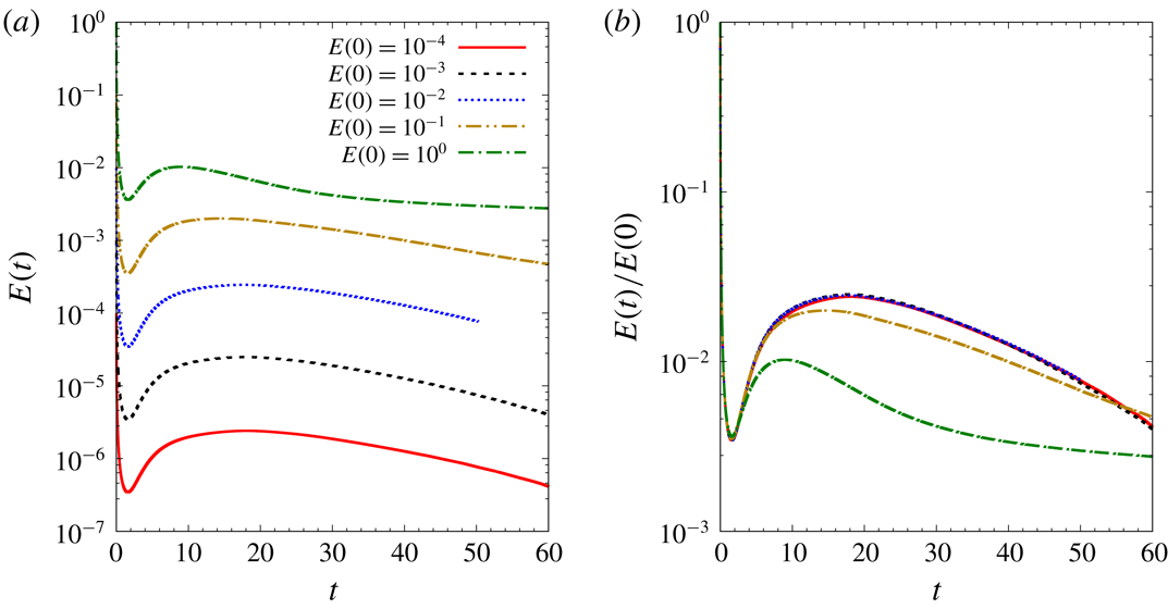If, on the other hand, the computation is initiated with a random perturbation that is localized in a similar spatial region of the computational domain as the LOP, and has initial energy $E(0)=10^{-4}$ , a different flow evolution is obtained. Figure 18(a) shows the variation of perturbation energy with time for a simulation initiated with an $E(0)=10^{-4}$ random perturbation. The energy initially decreases, exhibits transient growth for some time and then decreases monotonically with time. The level of perturbation energy is relatively low during the entire flow evolution. We recall from § 8 that the appearance of a helical displacement mode in the tip-vortex region is attributed to nonlinear effects. Because of low perturbation energy levels for a computation initiated with $E(0)=10^{-4}$ random perturbation, nonlinear effects are not significant. This is apparent in the absence of a helical perturbation inside the tip vortex (compare 19 a and bottom right panel of figure 16). Hence, for an $E(0)=10^{-4}$ random perturbation, no perceptible meandering of the vortex core occurs. With an increase in the value of $E(0)$ , nonlinear terms play an increasing role in modifying the shape of the perturbation (figure 19 b–e). For $E(0)\geqslant 0.01$ , the perturbation wavepacket within the tip-vortex region takes a helical shape (figure 19 c–e). In these situations, vortex displacement occurs. For $E(0)\leqslant 0.1$ , the energy of the perturbation wavepacket decreases as it travels downstream; no quasi-steady interval is observed. For higher $E(0)$ , the energy of the perturbation wavepacket appears to saturate in the wake (see energy gain curve for $E(0)=1.0$ in figure 18 a for $t\gtrsim 30$ ). The saturation is more apparent if we compare the plots of energy gain for different $E(0)$ random perturbations (figure 18 b).

To summarize, a random perturbation close to the wing leads to similar motion as the linear optimal perturbation, albeit with much higher initial energy. The role of the nonlinear process in shaping the perturbation wavepacket within the tip vortex is central to the occurrence of vortex displacement (which may be linked to the phenomenon of vortex meandering). Linear optimal perturbation extracts energy from the base flow in the most optimal way, and therefore, a nonlinear process is triggered with a relatively low value of initial energy as compared to a random perturbation.

9.2 Unsteady base flow regime

Figure 19.

$Re=1000$ flow past a flat plate wing with $\unicode[STIX]{x1D6FC}=5$ and $AR=6$ : isosurface of streamwise vorticity for the perturbation wavepacket obtained via nonlinear simulation. Random perturbation is used as the initial condition for the computation. The value of initial energy is (a) $E(0)=0.0001$ (b) $E(0)=0.001$ , (c) $E(0)=0.01$ , (d) $E(0)=0.1$ and (e) $E(0)=1.0$ . The position of the base flow tip vortex is indicated using dotted outline in (e).

The mechanism of vortex meandering proposed above is based on results in the flow regime where the base flow is steady ( $Re\leqslant 2500$ for the flat plate wing). We argue that the proposal holds even beyond the steady flow regime. In support of our argument, we consider the $Re=3000$ flow past a flat plate wing. For $Re=3000$ , the steady wake behind the wing is unstable. A Kármán vortex street exists in the wake up to a distance of ${\sim}20c$ from the leading edge of the wing (figure 6 b). Beyond $x\sim 20c$ , vortex shedding is suppressed and the flow becomes steady. We place a velocity probe inside the tip-vortex region at various streamwise locations. The velocity signal is recorded for a sufficiently large time so that the mean value of the signal becomes statistically invariant. The mean value is subtracted from the velocity signal, to obtain the time history of velocity fluctuation. Figure 20(a) shows spanwise velocity fluctuation at $x=15c$ . The frequency of fluctuation is found to be the same as the frequency of vortex shedding in the trailing edge wake. This suggests that velocity fluctuations within the tip vortex are linked to vortex shedding activity in the trailing edge wake. The fluctuation level decreases with streamwise distance. For $x=35c$ and $50c$ , fluctuations are negligible (figure 20 b,c). A numerical experiment is carried out where external perturbation is added periodically at an interval of 48 time units to $Re=3000$ flow. The perturbation is random and localized in the vicinity of the wing surface, and has relatively low initial energy ( $E(0)\sim 10^{-8}$ ). As for the unperturbed case, we record the velocity signal at various downstream locations and calculate its fluctuation about the mean. Figures 20(d)–20(f) show the spanwise velocity fluctuations at $x=15c$ , $35c$ and $50c$ , respectively for the situation where the perturbation is externally added. Periodic bursts are observed in the signal of velocity fluctuations. They are shown with broken rectangles in the three figures. The time period of the burst matches the period of addition of external perturbation to the flow. Each burst originates near the wing and travels downstream with a speed nearly the same as the free-stream speed. The relatively large value of the velocity fluctuation during the bursts suggests amplification of the initial perturbation which otherwise has small energy. The phase difference between spanwise and transverse components of the velocity fluctuation suggests that each burst is associated with elliptical motion of the tip vortex. Hence, similar to the steady flow regime, for the unsteady flow also, the perturbation near the wing surface amplifies in the near wake and travels downstream like a wavepacket causing displacement of tip vortices.

Figure 20.

$Re=3000$ flow past a flat plate with $\unicode[STIX]{x1D6FC}=5$ and $AR=6$ : time signal of spanwise velocity fluctuation at (a,d) $x=15c$ , (b,e) $x=35c$ and (c,f) $x=50c$ . The top row corresponds to the situation with no external perturbation, and the bottom row is for the case when perturbation is injected periodically into the flow near the wing surface. The bursts in the velocity signal arising from the addition of an external perturbation are shown by broken rectangles in (d–f).

We observe that the level of initial energy for a random perturbation to result in vortex meandering at $Re=3000$ is much lower than that at $Re=1000$ (figure 19). The reason may be attributed to an increase in the amplification of the initial perturbation energy with $Re$ . This has been shown to be the case in the steady flow regime where energy gain for LOP increases exponentially with $Re$ (table 2). We speculate that unsteadiness (laminar) does not affect the mechanism of amplification of initial perturbation energy. Consequently, the amplification of initial energy for $Re=3000$ is expected to be significantly higher than $Re=1000$ . Another observation that we make is that the presence of unsteadiness in the near wake (in the form of Kármán vortex shedding) alone does not result in perceptible meandering of the tip vortices. Therefore, the location of the perturbation is important for vortex motion (that resembles the phenomenon of vortex meandering).

10 Conclusions and perspectives

Optimal perturbation analysis for a trailing vortex system has been carried out in the linear framework using a direct–adjoint iterative procedure. While earlier studies have mostly considered a pair of counter-rotating vortices, our analysis takes into account, in addition to the tip vortex, the flow over the wing surface and the region of roll-up of the axial vorticity layer. From the computational point of view, the latter approach requires much larger resources owing to the requirement of adequate flow resolution in a large part of the wake that includes the vortex roll-up, unsteadiness (Kármán vortex street) and fully developed tip vortex. It is observed that beyond the vortex roll-up distance, the wake can be broadly divided into two parts: trailing edge wake (dominated by the spanwise component of vorticity), and tip vortex (dominated by the streamwise component of vorticity). The separation between the two parts of the wake increases downstream. With increase in $Re$ , the trailing edge wake becomes unsteady and then undergoes transition to a turbulent state. For a rectangular flat plate wing with $AR=6$ and $\unicode[STIX]{x1D6FC}=5^{\circ }$ , the trailing edge wake becomes turbulent between $3000<Re<5000$ . A more detailed analysis is required to determine the critical $Re$ for the onset of turbulence in this case. The tip vortex retains its laminar characteristics up to a much higher $Re$ than the trailing edge wake. For the aforementioned rectangular flat plate wing, the tip vortex is found to remain laminar up to $Re=5000$ .

Optimization has been carried out in the regime where the fully developed flow within the computational domain is steady. The study reveals that the steady base flow can support significant transient growth of the perturbation. Parametric exploration over $T$ , $Re$ , $AR$ and $\unicode[STIX]{x1D6FC}$ yields that the general shape of linear optimal perturbation (LOP) remains the same. LOP is found to be located near the wing surface and its shape suggests that the initial transient growth occurs via the Orr mechanism. The strength of LOP is largest near the symmetry plane. It decreases in the spanwise direction and is nearly zero at the wing-tip. For a given time horizon, linear optimal gain is found to increase with $Re$ , $AR$ and $\unicode[STIX]{x1D6FC}$ . A change in the sectional geometry from flat plate to NACA0012 (keeping $T$ , $Re$ , $AR$ and $\unicode[STIX]{x1D6FC}$ fixed) increases the value of linear optimal gain by an order of magnitude.

Long time evolution of a linear optimal perturbation is studied by direct time integration of the disturbance equations. Both linear and nonlinear evolution is simulated. In both situations, the perturbation evolves like a downstream travelling wavepacket whose energy increases in the near wake region via the Orr mechanism. It is found that nonlinear terms can have a significant effect on the evolution of the perturbation even with a relatively small value of the initial perturbation energy. The nonlinear wavepacket results in an elliptical motion of the tip vortex in the transverse plane. The linear wavepacket, on the other hand, does not cause any perceptible shift in the location of the vortex core. In the nonlinear simulation the energy of the perturbation wavepacket saturates beyond a certain streamwise location.

Nonlinear evolution of a random perturbation that is localized in the same spatial region as LOP is simulated and its results are compared with that obtained for nonlinear evolution of LOP. It is observed that the perturbation wavepacket generated via random initial perturbation requires a much higher value of initial energy than LOP to cause perceptible motion of the vortex core. LOP, therefore, extracts energy from the base flow in the most optimal way that can cause movement of the vortex core with a relatively low value of the initial energy. When the flow becomes unsteady, it is observed that a random perturbation near the wing surface with relatively low initial energy can trigger vortex displacement. Our results highlight the high sensitivity of the vortex motion to perturbations located at the wing surface. In particular, our analysis suggests that near wake energy amplification and nonlinear effects might be central to the phenomenon of vortex meandering.

The fact that LOP is localized near the wing is desirable from the point of view of wake control as the wing provides a physical surface for placing the control actuators. This, coupled with the observation that during its evolution LOP can displace the tip vortex in the transverse plane, suggests that LOP may be useful in designing control strategies for hastening the onset of the Crow instability in a trailing vortex system. A proposal in this direction is periodic injection of LOP with a frequency corresponding to the wavelength of the Crow instability.

The significance of nonlinear effects on the evolution of perturbation provides a motivation to carry out nonlinear optimization for the flow past a finite wing. In a recent work (Navrose et al. Reference Navrose, Brion, Jacquin and Robinet2018), we have shown that a nonlinear optimal perturbation can result in significantly higher gain than the linear optimal gain for a 2-D isolated vortex and counter-rotating vortex pair. The flow evolution obtained using the nonlinear optimal perturbation as the initial condition, brings out new and interesting dynamics of the flow system, for example the appearance of a non-axisymmetric vortex state. Compared to linear optimization, nonlinear optimization is more demanding on computational resources. This is because, unlike linear optimization, nonlinear optimization using a direct–adjoint iterative technique requires information of direct variables to be saved at each time step of an iteration. This not only increases the requirement of disk space, but also increases the computational time owing to reading and writing of data on the disks. Another challenging aspect of nonlinear optimization is its slow convergence as compared to linear simulation. Typically, the number of iterations required for nonlinear optimization is an order of magnitude higher than that for linear optimization. Kerswell (Reference Kerswell2018) has summarized some of the challenges involved in nonlinear optimization of large problems. With ongoing development of computational tools and resources, nonlinear optimization using the full flow field can be attempted in the future. The nonlinear framework is also expected to reveal the significance of interaction between symmetric and anti-symmetric perturbation.

The evolution of LOP as a nonlinear wavepacket that results in displacement of the vortex core has been proposed as a possible mechanism behind vortex meandering. The role of LOP is to cause optimal amplification of initial perturbation that allows suitable modification of the shape of the perturbation wavepacket via nonlinear effects. A question that arises here is: what is the source of LOP is experiments? Fontane et al. (Reference Fontane, Fabre and Brancher2008) studied the dynamics of a vortex column in the presence of stochastic forcing and showed that the most receptive flow structure resembles the optimal perturbation for an isolated vortex. The justification for using stochastic forcing was to emulate the effect of external noise that is generally present is experiments. Schrader et al. (Reference Schrader, Brandt and Henningson2009) investigated receptivity mechanisms in boundary layer and suggested that free-stream turbulence can interact with a steady perturbation source like surface roughness and trigger natural instability of the flow. We speculate that perturbation sources near the wing (for example, turbulence at the wing boundary layer, surface macro-roughness and/or wing deformation) might excite disturbances resembling LOP.

We close this section with a note on the applicability of the results presented in this paper. The numerical simulations have been carried out for an $Re$ -range ( $1000\leqslant Re\leqslant 3000$ ) that is several orders of magnitude lower than that encountered in practical situations ( $Re\sim \mathit{O}(10^{6})$ ). A question then arises is, are the results presented in the paper practically significant? To this, we point out that in many practical scenarios the wing-tip vortex has a laminar core (Cotel & Breidenthal Reference Cotel and Breidenthal1999) and its structure is similar to that obtained in the present work. A comparison between the velocity profile of the tip vortex obtained via numerical simulation and large- $Re$ laminar vortex models is presented in the Appendix. The similarity in the structure of low- and large- $Re$ vortices suggests that the dynamics of the wing-tip vortex brought out in the present work might be observed in practice as well. This serves as a motivation for carrying out transient growth analysis in the large- $Re$ flow regime. Since the trailing edge wake becomes turbulent with an increase in $Re$ , a different technique than the one used in the present work might be needed, for example, using mean flow as the base solution for optimization. Transient growth analysis using mean flow has been carried out in the past for turbulent flow systems like channel and boundary layer flow (del Álamo & Jiménez Reference del Álamo and Jiménez2006; Cossu, Pujals & Depardon Reference Cossu, Pujals and Depardon2009). The mean flows in such works have mostly been obtained via RANS (Reynolds-averaged Navier–Stokes) simulation. However, the standard turbulence models employed for RANS simulations might be inadequate for flows with curvature like wing-tip vortex, and hence require correction (Dacles-Mariani et al. Reference Dacles-Mariani, Zilliac, Chow and Bradshaw1995; Shur et al. Reference Shur, Strelets, Travin and Spalart2000). The validity of RANS models in simulation of trailing vortices up to large distances from the wing, as attempted in the present study, has received less attention as compared to other flows. Two works in this direction are by Zeman (Reference Zeman1995) and Czech et al. (Reference Czech, Miller, Crouch and Strelets2004). Czech et al. (Reference Czech, Miller, Crouch and Strelets2004), in particular, validated RANS model by comparing numerical results obtained using parabolized simulations with experimental data. Another approach for obtaining the mean flow could be large eddy simulation (LES) for the flow past a wing. This, however, might present challenges in terms of computational cost, especially if a parametric study, as carried out in the present work, is undertaken.