1. Introduction
In many shallow coastal environments, sediment transport is often due to the combined action of surface waves and steady currents. The oscillatory flow induced by wave propagation contributes substantially to the pick-up of sediment from the bottom. Then, even though a net flux of sediment can also be induced by the waves because of the steady streaming effects and the possible asymmetry of the velocity oscillations, the largest contribution to the sediment transport is possibly induced by the currents, which steadily drag the sediment in their direction.
In the modelling of the sediment transport a major role is played by accurate evaluation of the bottom shear stress and flow in the bottom boundary layer (Blondeaux & Vittori Reference Blondeaux and Vittori1999). Hence, a large number of studies have been devoted to the study of flow in the boundary layer generated close to the bottom by the interaction of a wave train and a steady current. Attention has been focused on the turbulent regime, and turbulence models of different complexity have been used. Some of them are described in the review paper by Soulsby et al. (Reference Soulsby, Hamm, Klopman, Myrhaug, Simons and Thomas1993), who summarize the results obtained in the framework of a research project funded by the EU. Turbulent stresses are usually evaluated by introducing an eddy viscosity and using either analytical models or numerical approaches to solve momentum and continuity equations. The most common models assume that the turbulence characteristics depend on either one or two scalar quantities which are evaluated by solving advection–diffusion equations. Let us mention the models of Grant & Madsen, (Reference Grant and Madsen1979, Reference Grant and Madsen1986), Fredsøe (Reference Fredsøe1984), Davies, Soulsby & King (Reference Davies, Soulsby and King1988) and the more recent paper by Olabarrieta, Medina & Castanedo (Reference Olabarrieta, Medina and Castanedo2010), where other recent contributions to the study of wave–current interaction are presented and discussed.
However, in shallow sedimentary environments characterized by a very fine sediment, significant sediment concentrations are also found far from the bottom, and knowledge of the flow in the entire water column is quite important to the quantification of the sediment transport rate (Vittori Reference Vittori2003). Hence, it is crucial to understand the interaction between waves and currents not only close to the bottom but also far from it.
The experimental investigations of wave–current interaction show significant reduction of the current velocity near the free surface when the waves propagate in the direction of the current, whereas the current velocity increases near the free surface when the waves propagate in the opposite direction; see, among others, Kemp & Simons (Reference Kemp and Simons1982, Reference Kemp and Simons1983), Klopman (Reference Klopman1994, Reference Klopman1997), Umeyama (Reference Umeyama2005) and references therein.
In order to study wave–current interaction theoretically, the hydrodynamic problem can be formulated using either an Eulerian approach or a Lagrangian approach (Dingemans et al. Reference Dingemans, Van Kester, Radder and Uittenbogaard1996; Groeneweg & Klopman Reference Groeneweg and Klopman1998; Groeneweg & Battjes Reference Groeneweg and Battjes2003). Using an Eulerian model, Nielsen & You (Reference Nielsen and You1996) introduced several ad hoc assumptions and proposed an eddy viscosity model which allowed them to obtain fair results, even though, as pointed out by Huang & Mei (Reference Huang and Mei2003), the agreement between the experimental data and theoretical predictions was not entirely satisfactory. More recently, interaction between waves and current was studied by Huang & Mei (Reference Huang and Mei2003), who quantified the turbulent stresses by using an algebraic turbulence model which provides the eddy viscosity directly from the flow variables. However, the analysis of Huang & Mei (Reference Huang and Mei2003) is not simple to apply, since it is based on a perturbation approach which splits the fluid domain into an inviscid core region and viscous boundary layers and relates the order of magnitude of some quantities (e.g. the shear velocities, the bottom roughness, and the components of the stress tensor) to the wave steepness. Moreover, the approach requires us to consider vorticity dynamics within the core region, where the vorticity distribution depends on a balance between viscous and convective effects. This makes it hard to extend the analysis to currents that form an arbitrary angle with the direction of wave propagation.
The hydrodynamic problem was also solved by Olabarrieta et al. (Reference Olabarrieta, Medina and Castanedo2010) by means of a numerical approach. The numerical solution is able to take into account nonlinear terms without assuming small values of the wave steepness. Moreover, the introduction of time-dependent coordinate stretching allows the boundary condition to be applied exactly at the free surface. However, some approximation has to be introduced in any case (e.g. nonlinear effects in the vertical component of momentum equations are neglected), and the numerical solution implies high computational costs which, in this case too, make it quite hard to consider arbitrary angles between the direction of the current and that of wave propagation.
Quite often, the depth-averaged velocity due to the current has the same order of magnitude as the amplitude of the velocity oscillations induced by the wave propagation, and both velocities can be assumed to be much smaller than the wave celerity. It follows that the flow field generated by the wave–current interaction can be determined by expanding it using the wave steepness
 $a$
as a small parameter. The problems which should be solved at different orders of approximation are characterized by a further small parameter
 ${\it\delta}_{T}$
, which can be thought of as the ratio between the order of magnitude of the viscous effects and that of the local acceleration term. The small values of
 ${\it\delta}_{T}$
would suggest the use of an inviscid approach to the study of wave propagation, and the introduction of bottom and surface boundary layers to allow the wave solution to satisfy all the boundary conditions. However, as already pointed out, such an approach is difficult to apply when the direction of the wave propagation forms an arbitrary angle with the direction of the current. Moreover, this approach makes it necessary to introduce further simplifying assumptions.
In the present analysis, to avoid the decomposition of the fluid domain into an inviscid core region and viscous boundary layers, we propose an approach which provides the flow field generated by the interaction of waves and currents in the entire water column. We consider a coastal region characterized by a constant finite depth, and we assume the depth-averaged velocity of the steady current to be of the same order of magnitude as the amplitude of the velocity oscillations induced by the wave propagation, and both velocities to be much smaller than the wave celerity. Reynolds stresses are quantified by introducing the Boussinesq model and an eddy viscosity which is assumed to depend on the shear velocity and on the distance from the bottom and the free surface. Even though one can criticize this simple turbulence model when it is applied to oscillatory flows, comparison of the results it provides with the laboratory measurements of Kemp & Simons (Reference Kemp and Simons1982, Reference Kemp and Simons1983), Klopman (Reference Klopman1994, Reference Klopman1997) and Umeyama (Reference Umeyama2005) shows that the model can provide a reliable description of the phenomenon. Moreover, the reader should take into account that the analysis can be easily modified by introducing other turbulence models.
The next section describes the hydrodynamic problem. Then, § 3 summarizes the procedure employed to solve the problem. The results are presented and discussed in § 4. Finally, § 5 is devoted to the conclusions.
2. Formulation of the problem
Let us consider a coastal region of constant water depth
 $h^{\ast }$
, characterized by the presence of a monochromatic surface gravity wave of angular frequency
 ${\it\omega}^{\ast }$
, which propagates in the negative
 $x^{\ast }$
direction, and by a steady current which forms an arbitrary angle with the
 $x^{\ast }$
direction (a star denotes dimensional quantities while the same symbol without the star indicates its dimensionless counterpart). Let us complete the definition of the Cartesian coordinate system by introducing the vertical
 $z^{\ast }$
axis, which points upward, so that
 $z^{\ast }=0$
describes the still water level.
At this stage, it is convenient to introduce dimensionless variables. The quantities
 $1/k^{\ast }=L^{\ast }/2{\rm\pi}$
and
 $1/{\it\omega}^{\ast }=T^{\ast }/2{\rm\pi}$
are used as spatial and temporal scales, respectively,
 $L^{\ast }$
and
 $T^{\ast }$
being the length and the period of the surface waves, which are provided by the linear Stokes theory and satisfy the dispersion relation
 ${\it\omega}^{\ast 2}=g^{\ast }k^{\ast }\tanh (k^{\ast }h^{\ast })$
. Moreover, the quantity
 $U_{0}^{\ast }=a^{\ast }{\it\omega}^{\ast }/\text{sinh}(k^{\ast }h^{\ast })$
is used as velocity scale and
 $a^{\ast }$
denotes the amplitude of the waves:
 $$\begin{eqnarray}\displaystyle \left.\begin{array}{@{}c@{}}\displaystyle (x,y,z)=k^{\ast }(x^{\ast },y^{\ast },z^{\ast }),\quad t={\it\omega}^{\ast }t^{\ast },\quad (u,v,w)=\frac{(u^{\ast },v^{\ast },w^{\ast })}{U_{0}^{\ast }},\\ \displaystyle P=\frac{P^{\ast }k^{\ast }S}{{\it\rho}^{\ast }a^{\ast }{\it\omega}^{\ast 2}},\quad {\it\eta}=\frac{{\it\eta}^{\ast }}{a^{\ast }}.\end{array}\right\} & & \displaystyle\end{eqnarray}$$
Here
 ${\it\rho}^{\ast }$
denotes the fluid density,
 $(u^{\ast },v^{\ast },w^{\ast })$
are the Reynolds-averaged velocity components in the
 $(x^{\ast },y^{\ast },z^{\ast })$
directions, respectively,
 ${\it\eta}^{\ast }$
is the free surface elevation, and the modified pressure
 $P^{\ast }$
is defined by
 $P^{\ast }=p^{\ast }+{\it\rho}^{\ast }g^{\ast }z^{\ast }$
,
 $p^{\ast }$
being the actual pressure in the fluid. Moreover,
 $S$
denotes the quantity
 $\sinh (k^{\ast }h^{\ast })$
.
The dimensionless hydrodynamic problem is posed by the continuity and momentum equations
 $$\begin{eqnarray}\displaystyle & & \displaystyle \frac{\partial u}{\partial x}+\frac{\partial v}{\partial y}+\frac{\partial w}{\partial z}=0\end{eqnarray}$$
 $$\begin{eqnarray}\displaystyle & & \displaystyle \frac{\partial u}{\partial t}+a\left[u\frac{\partial u}{\partial x}+v\frac{\partial u}{\partial y}+w\frac{\partial u}{\partial z}\right]=-\frac{\partial P}{\partial x}+\,\frac{{\it\delta}_{T}^{2}}{2}\left\{\frac{\partial }{\partial x}\left[2({\it\nu}+{\it\nu}_{T})\frac{\partial u}{\partial x}\right]\right.\nonumber\\ \displaystyle & & \displaystyle \qquad +\left.\frac{\partial }{\partial y}\left[({\it\nu}+{\it\nu}_{T})\left(\frac{\partial u}{\partial y}+\frac{\partial v}{\partial x}\right)\right]+\frac{\partial }{\partial z}\left[({\it\nu}+{\it\nu}_{T})\left(\frac{\partial u}{\partial z}+\frac{\partial w}{\partial x}\right)\right]\right\}\end{eqnarray}$$
 $$\begin{eqnarray}\displaystyle & & \displaystyle \frac{\partial v}{\partial t}+a\left[u\frac{\partial v}{\partial x}+v\frac{\partial v}{\partial y}+w\frac{\partial v}{\partial z}\right]=-\frac{\partial P}{\partial y}+\frac{{\it\delta}_{T}^{2}}{2}\left\{\frac{\partial }{\partial x}\left[({\it\nu}+{\it\nu}_{T})\left(\frac{\partial u}{\partial y}+\frac{\partial v}{\partial x}\right)\right]\right.\nonumber\\ \displaystyle & & \displaystyle \qquad +\left.\frac{\partial }{\partial y}\left[2({\it\nu}+{\it\nu}_{T})\frac{\partial v}{\partial y}\right]+\frac{\partial }{\partial z}\left[({\it\nu}+{\it\nu}_{T})\left(\frac{\partial v}{\partial z}+\frac{\partial w}{\partial y}\right)\right]\right\}\end{eqnarray}$$
 $$\begin{eqnarray}\displaystyle & & \displaystyle \frac{\partial w}{\partial t}+a\left[u\frac{\partial w}{\partial x}+v\frac{\partial w}{\partial y}+w\frac{\partial w}{\partial z}\right]=-\frac{\partial P}{\partial z}+\frac{{\it\delta}_{T}^{2}}{2}\left\{\frac{\partial }{\partial x}\left[({\it\nu}+{\it\nu}_{T})\left(\frac{\partial u}{\partial z}+\frac{\partial w}{\partial x}\right)\right]\right.\nonumber\\ \displaystyle & & \displaystyle \qquad +\left.\frac{\partial }{\partial y}\left[({\it\nu}+{\it\nu}_{T})\left(\frac{\partial v}{\partial z}+\frac{\partial w}{\partial y}\right)\right]+\frac{\partial }{\partial z}\left[2({\it\nu}+{\it\nu}_{T})\frac{\partial w}{\partial z}\right]\right\},\end{eqnarray}$$
 ${\it\nu}={\it\nu}^{\ast }/\hat{{\it\nu}}_{T0}^{\ast }$
denotes the dimensionless kinematic viscosity of the water, and the dimensionless eddy viscosity
 ${\it\nu}_{T}={\it\nu}_{T}^{\ast }/\hat{{\it\nu}}_{T0}^{\ast }$
is introduced to quantify the Reynolds stresses. The quantity
 $\hat{{\it\nu}}_{T0}^{\ast }$
, which is used to scale the eddy viscosity, is assumed to be equal to
 ${\it\kappa}\sqrt{f_{cw}/2}U_{0}^{\ast }h^{\ast }$
, where
 ${\it\kappa}=0.4$
is the von Kármán constant and
 $f_{cw}$
is a friction coefficient. To obtain the results discussed below, the friction coefficient is quantified by using either the procedure described in Soulsby (Reference Soulsby1997) for the wave–current case or the empirical relationship proposed by Marchi (Reference Marchi1961a
,Reference Marchi
b
), which provides
 $C=\sqrt{2/f_{cw}}$
as a function of the bottom roughness and the Reynolds number, for currents alone. The velocity profiles turn out to be indistinguishable. Indeed, the value of the friction coefficient does not affect the velocity profile but only the pressure gradient needed to drive the steady current. However, since no measurement of the free surface slope is available to compare with, it is not possible to single out the best formula to predict
 $f_{cw}$
. This finding is similar to what is found for steady currents without waves: if the eddy viscosity is assumed to scale with the friction velocity and the water depth and its vertical profile is fixed, the velocity profile, once scaled with the friction velocity, does not depend on the bottom roughness. In other words, the roughness size affects only the surface slope needed to drive the given flow rate.
In (2.2)–(2.5), two parameters appear, namely
 $$\begin{eqnarray}\displaystyle a=\frac{a^{\ast }k^{\ast }}{S},\quad {\it\delta}_{T}=\sqrt{\frac{2\hat{{\it\nu}}_{T0}^{\ast }k^{\ast 2}}{{\it\omega}^{\ast }}}. & & \displaystyle\end{eqnarray}$$
Moreover, the forcing terms
 $-\partial P/\partial x$
,
 $-\partial P/\partial y$
and
 $-\partial P/\partial z$
should have a steady part, which drives the steady current, and an oscillatory part, which is generated by the propagation of the surface wave.
At the bottom, described by
 $z=-h=-k^{\ast }h^{\ast }$
, the no-slip condition forces the vanishing of the velocity components. At the free surface, described by
 $z=aS{\it\eta}(x,y,t)$
, the dimensionless kinematic boundary condition reads
 $$\begin{eqnarray}\displaystyle \frac{\partial {\it\eta}}{\partial t}+a\left[u\frac{\partial {\it\eta}}{\partial x}+v\frac{\partial {\it\eta}}{\partial y}\right]-\frac{w}{S}=0, & & \displaystyle\end{eqnarray}$$
while the dynamic boundary conditions force the tangential stresses to vanish and the normal stress to balance the atmospheric pressure, since the surface tension effects are neglected by assuming that the Weber number of the phenomenon is sufficiently large.
To close the problem, it is necessary to introduce a turbulence model to provide the value of the eddy viscosity. To keep the analysis as simple and transparent as possible, the eddy viscosity
 ${\it\nu}_{T}^{\ast }$
is assumed to depend on the distance from the bottom only. Indeed, even though the actual eddy viscosity depends on time because of the fluid oscillations, two-equation turbulence models (e.g. Blondeaux Reference Blondeaux1987) show that the oscillations of the viscosity are significantly smaller than its time-averaged value and a time-independent value of
 ${\it\nu}_{T}^{\ast }$
provides a reasonable description of the turbulent mixing.
Laboratory observations show that the eddy viscosity increases almost linearly with
 $z^{\ast }$
when the region close to the bottom is considered (see for example the book by Nielsen Reference Nielsen1992). Then, moving far from the bottom, the growth of
 ${\it\nu}_{T}^{\ast }$
slows down and a maximum value is attained in the upper part of the water column. Indeed,
 ${\it\nu}_{T}^{\ast }$
decreases and tends to vanish moving towards the free surface, even when a steady current is present (Bakker and Van Doorn Reference Bakker and Van Doorn1978; Kim et al.
Reference Kim, O’Conner, Park and Lee2001; Nezu & Rodi Reference Nezu and Rodi1986).
Following previous algebraic models of turbulence generated by the interaction of waves and currents (see for example the book by Fredsøe & Deigaard Reference Fredsøe and Deigaard1992), in the present analysis, different values are given to
 ${\it\nu}_{T}^{\ast }$
in the bottom boundary layer and in the core region. In the bottom boundary layer the eddy viscosity is assumed to be proportional to the amplitude of the shear velocity oscillations. Outside the boundary layer, the eddy viscosity is assumed to be proportional to the time-averaged shear velocity
 $$\begin{eqnarray}\displaystyle {\it\nu}_{T} & = & \displaystyle \frac{F({\it\zeta})}{2\sqrt{f_{cw}/2}}\left\{\sqrt{{\it\tau}_{max}}\left[1-\tanh \left(\frac{c_{3}({\it\zeta}-{\it\delta}_{w})}{{\it\delta}_{w}}\right)\right]\right.\nonumber\\ \displaystyle & & \displaystyle +\,\left.\sqrt{{\it\tau}_{steady}}\left[1+\tanh \left(\frac{c_{3}({\it\zeta}-{\it\delta}_{w})}{{\it\delta}_{w}}\right)\right]\right\},\end{eqnarray}$$
where
 $$\begin{eqnarray}\displaystyle F({\it\zeta})=c_{1}{\it\zeta}\left[1-\text{exp}\left(-c_{2}\left(1-{\it\zeta}\right)\right)\right]\quad \text{with }{\it\zeta}=1+\frac{z}{h}. & & \displaystyle\end{eqnarray}$$
Moreover,
 ${\it\delta}_{w}=2{\it\kappa}a\sqrt{{\it\tau}_{max}}$
is a measure of the thickness of the oscillatory boundary layer,
 ${\it\kappa}$
is the von Kármán constant,
 ${\it\tau}_{max}$
is the maximum value of the bottom shear stress induced during the wave cycle and
 ${\it\tau}_{steady}$
is the time-averaged value of the bottom shear stress. The value of
 ${\it\delta}_{w}$
is obtained by assuming that
 ${\it\delta}_{w}^{\ast }=(2\hat{{\it\nu}}_{T}^{\ast }/{\it\omega}^{\ast })^{1/2}$
, where
 $\hat{{\it\nu}}_{T}^{\ast }$
is given by
 ${\it\kappa}({\it\tau}_{max}^{\ast }/{\it\rho}^{\ast })^{1/2}{\it\delta}_{w}^{\ast }$
. The constant
 $c_{1}=2.65$
is chosen in such a way that
 $\int _{0}^{1}F({\it\zeta})\,\text{d}{\it\zeta}=1$
. Indeed,
 $F({\it\zeta})$
should describe only the dependence of the eddy viscosity on the vertical coordinate, while its magnitude is provided by
 $\hat{{\it\nu}}_{T0}^{\ast }$
. The constant
 $c_{2}$
is set equal to
 $7$
in such a way that the maximum value of
 $F$
is attained at about a quarter of the water depth, as in Olabarrieta et al. (Reference Olabarrieta, Medina and Castanedo2010). Finally,
 $c_{3}$
is fixed equal to
 $10$
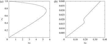
in such a way that the eddy viscosity assumes the vertical profile previously described and sketched in figure 1, but it is not discontinuous at the top of the boundary layer. The value of the constant
 $c_{3}$
has no significant effect on the results as long as its value ensures the smoothness of
 ${\it\nu}_{T}(z)$
. At this stage it is worth pointing out that small variations of
 $F({\it\zeta})$
do not significantly affect the results described below. In particular, values different from zero can be given to
 $F(1)$
as long as
 $F(1)$
is relatively small.
Vertical profile of the eddy viscosity for
 ${\it\tau}_{max}=0.055,{\it\tau}_{steady}=0.03,f_{cw}=0.00535,a=0.096$
, which are the values of the parameter characteristics of Klopman’s (Reference Klopman1994) experiments with regular waves. Only the enlargement of the region close to the bottom (b) clarifies the differences between the eddy viscosity within the bottom boundary layer and the eddy viscosity outside the bottom boundary layer.

3. The solution
If the amplitude
 $a^{\ast }$
of the wave is assumed to be much smaller than its wavelength, and the velocity induced by the current is assumed to be of the same order of magnitude as the amplitude of the velocity oscillations induced by wave propagation (or equivalently the celerity of the surface wave is assumed to be much larger than both the velocity oscillations induced by the waves and the current velocity), the solution can be expanded in the form
 $$\begin{eqnarray}\displaystyle (u,v,w,P,{\it\eta})=(u_{0},v_{0},w_{0},P_{0},{\it\eta}_{0})+a(u_{1},v_{1},w_{1},P_{1},{\it\eta}_{1})+O(a^{2}). & & \displaystyle\end{eqnarray}$$
The hydrodynamic problems, which are obtained at order
 $a^{0}$
and at order
 $a^{1}$
, are characterized by the presence of the parameter
 ${\it\delta}_{T}$
, which a preliminary estimation (based on typical values of the parameters for sea waves) shows to be much smaller than one and also smaller than the wave steepness
 $a$
. If the velocity field is divided into a steady part and an oscillatory part, the presence of the small parameter
 ${\it\delta}_{T}$
, which multiplies the highest derivatives appearing in problems for the oscillatory velocity component, would suggest solution by considering the inviscid momentum equations far from the bottom, and matching the inviscid solutions with solutions that are valid in ‘viscous’ bottom boundary layers close to the bottom and close to the free surface. Moreover, the determination of the steady velocity component, induced by wave propagation, in the inviscid region would require us to consider the time average of the vorticity equation, which gives rise to a balance between convective and viscous effects and provides results that depend on the ratio between
 $a$
and
 ${\it\delta}_{T}$
. However, the appendix of the paper by Blondeaux & Vittori (Reference Blondeaux and Vittori1994) shows that keeping the viscous
 $O({\it\delta}_{T}^{2})$
terms in momentum equations and integrating the equations from the bottom up to the free surface is equivalent to a formal matched asymptotic expansion. Hence, the problems are solved as described as follows.
First, the variables
 $\tilde{u} _{0},\tilde{w}_{0},\tilde{{\it\eta}}_{0},\tilde{u} _{1},\tilde{w}_{1},\tilde{{\it\eta}}_{1}$
are introduced such that
 $$\begin{eqnarray}\displaystyle \tilde{u} _{0}=u_{0}-\hat{u} _{0},\quad \tilde{w}_{0}=w_{0}-{\hat{w}}_{0},\quad \tilde{P}_{0}=P_{0}-\hat{P}_{0},\quad \tilde{{\it\eta}}_{0}={\it\eta}_{0}-\hat{{\it\eta}}_{0}, & & \displaystyle\end{eqnarray}$$
 $$\begin{eqnarray}\displaystyle \tilde{u} _{1}=u_{1}-\hat{u} _{1},\quad \tilde{w}_{1}=w_{1}-{\hat{w}}_{1},\quad \tilde{P}_{1}=P_{1}-\hat{P}_{1},\quad \tilde{{\it\eta}}_{1}={\it\eta}_{1}-\hat{{\it\eta}}_{1}, & & \displaystyle\end{eqnarray}$$
where
 $$\begin{eqnarray}\displaystyle (\hat{u} _{0},{\hat{w}}_{0},\hat{P}_{0},\hat{{\it\eta}}_{0})=(\cosh (z+h),-\text{i}\sinh (z+h),-\cosh (z+h),-1){\textstyle \frac{1}{2}}\text{e}^{i(t+x)}+\text{c.c.}, & & \displaystyle\end{eqnarray}$$
 $$\begin{eqnarray}\displaystyle (\hat{u} _{1},{\hat{w}}_{1},\hat{{\it\eta}}_{1}) & = & \displaystyle (-3\cosh [2(z+h)],3\text{i}\sinh [2(z+h)],\cosh (h)[2+\cosh (2h)])\nonumber\\ \displaystyle & & \displaystyle \times \,\frac{\text{e}^{2\text{i}(t+x)}}{8S^{2}}+\text{c.c.},\end{eqnarray}$$
 $$\begin{eqnarray}\displaystyle \hat{P}_{1}=(3\cosh [2(z+h)]-S^{2})\frac{\text{e}^{2\text{i}(t+x)}}{8S^{2}}+\frac{1}{8}(1-\cosh [2(z+h)])+\text{c.c.} & & \displaystyle\end{eqnarray}$$
are the solutions of the inviscid equations (
 $\text{c.c.}$
stands for the complex conjugate of the previous term) and describe the irrotational flow field generated by a surface wave propagating over a constant water depth. In particular, (3.4) describes a linear Stokes wave and (3.5)–(3.6) take into account nonlinear effects in the propagation of the wave.
Then, the variable
 ${\it\theta}=t+x$
, which is known as wave phase, is introduced.
Assuming that the velocity field does not depend on
 $y$
and neglecting terms of order
 ${\it\delta}_{T}$
and
 ${\it\delta}_{T}^{2}$
, substitution of (3.1) into continuity and momentum equations leads to two hydrodynamic problems at
 $O(a^{0})$
and
 $O(a)$
. In these problems the quantities
 ${\it\nu}_{T0}$
and
 ${\it\nu}_{T1}$
appear, which can be obtained by expanding, in terms of the parameter
 $a$
, the values of
 ${\it\tau}_{max}$
and
 ${\it\tau}_{steady}$
, computed by means of the constitutive relationship, and then the value of
 ${\it\nu}_{T}$
provided by (2.8). Since the procedure is long and tedious but straightforward, the details of the procedure are not given here, for brevity. Let us only point out that
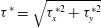 ${\it\tau}^{\ast }=\sqrt{{\it\tau}_{x}^{\ast 2}+{\it\tau}_{y}^{\ast 2}}$
and the components
 ${\it\tau}_{x}^{\ast }$
and
 ${\it\tau}_{y}^{\ast }$
of the bottom shear stress turn out to be equal to
 ${\it\mu}^{\ast }\partial u^{\ast }/\partial z^{\ast }|_{z^{\ast }=0}$
and
 ${\it\mu}^{\ast }\partial v^{\ast }/\partial z^{\ast }|_{z^{\ast }=0}$
, because of the vanishing of the eddy viscosity at the bottom. Hence,
 ${\it\tau}_{x0}^{\ast }={\it\mu}^{\ast }\partial u_{0}^{\ast }/\partial z^{\ast }|_{z^{\ast }=0}$
,
 ${\it\tau}_{x1}^{\ast }={\it\mu}^{\ast }\partial u_{1}^{\ast }/\partial z^{\ast }|_{z^{\ast }=0}$
,
 ${\it\tau}_{y0}^{\ast }={\it\mu}^{\ast }\partial v_{0}^{\ast }/\partial z^{\ast }|_{z^{\ast }=0}$
,
 ${\it\tau}_{y1}^{\ast }={\it\mu}^{\ast }\partial v_{1}^{\ast }/\partial z^{\ast }|_{z^{\ast }=0}$
. Then, the maximum value of the bottom shear stress and its time-averaged value can be easily determined once the flow field is known.
3.1.
 $O(a^{0})$
problem

At the leading order of approximation, the momentum equation in the direction of wave propagation becomes
 $$\begin{eqnarray}\displaystyle \frac{\partial \tilde{u} _{0}}{\partial {\it\theta}}=-\frac{\partial \tilde{P}_{0}}{\partial {\it\theta}}+\frac{{\it\delta}_{T}^{2}}{2}\frac{\partial }{\partial z}\left[\left({\it\nu}+{\it\nu}_{T0}\right)\frac{\partial \left(\hat{u} _{0}+\tilde{u} _{0}\right)}{\partial z}\right], & & \displaystyle\end{eqnarray}$$
while the momentum equation in the
 $y$
direction becomes
 $$\begin{eqnarray}\displaystyle \frac{\partial v_{0}}{\partial {\it\theta}}=-\frac{\partial \tilde{P}_{0}}{\partial y}+\frac{{\it\delta}_{T}^{2}}{2}\frac{\partial }{\partial z}\left[\left({\it\nu}+{\it\nu}_{T0}\right)\frac{\partial v_{0}}{\partial z}\right]. & & \displaystyle\end{eqnarray}$$
Even though, as already pointed out,
 ${\it\delta}_{T}$
is assumed to be much smaller than
 $a$
, the viscous terms in (3.7) and (3.8) are retained because they turn out to be significant within the bottom and surface boundary layers. Incidentally, let us point out that the viscous boundary layer at the free surface is neglected since, as pointed out by Huang & Mei (Reference Huang and Mei2003), it is much weaker than that at the bottom. Equations (3.7) and (3.8) are solved numerically by means of a finite difference approach to obtain
 $\tilde{u} _{0}$
and
 $v_{0}$
, once a constant value is given to
 $\partial \tilde{P}_{0}/\partial {\it\theta}$
and
 $\partial \tilde{P}_{0}/\partial y$
to drive the steady current (
 $\partial \tilde{P}_{0}/\partial {\it\theta}=S_{x},\partial \tilde{P}_{0}/\partial y=S_{y}$
).
As already pointed out, the diffusive terms in the horizontal directions
 $x$
and
 $y$
are neglected because of the small values of the parameter
 ${\it\delta}_{T}$
, while diffusive terms in the vertical direction are retained because the large velocity gradient, which characterizes the velocity profile close to the bottom, making them significant and as large as the other terms appearing in (3.7) and (3.8) when the region close to the bottom is considered.
A second-order central finite difference scheme is used to approximate the derivatives along a new coordinate
 $Z(z)=\text{arctanh}[c_{4}(2z/h+1)]$
, which is introduced to stretch the regions close to the bottom and the free surface, where the velocity gradient is expected to be larger (
 $c_{4}$
is a constant which should be properly chosen). The function
 $\tilde{u} _{0}$
turns out to depend on the wave phase
 ${\it\theta}$
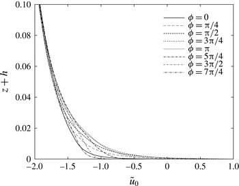
only in the viscous boundary layers close to the bottom and the free surface, where it turns out to be a periodic function. Figure 2 shows
 $\tilde{u} _{0}$
in the region close to the bottom for different values of the wave phase
 ${\it\theta}$
, the parameters being fixed equal to those characterizing Klopman’s (Reference Klopman1994) experiments with a monochromatic wave. The reader should notice that
 $\tilde{u} _{0}$
does not vanish at the bottom but oscillates between
 $-1$
and
 $1$
, since
 $\tilde{u} _{0}$
is the actual velocity minus the irrotational velocity induced by the wave propagation.
Values of
 $\tilde{u} _{0}$
for different wave phases in the region close to the bottom. The values of the parameters are equal to those of Klopman’s (Reference Klopman1994) experiments with a monochromatic wave, i.e.
 $h^{\ast }=0.5~\text{m}$
,
 $a^{\ast }=6~\text{cm}$
,
 $T^{\ast }=1.44~\text{s}$
.

Then the determination of the function
 $\tilde{w}_{0}$
can be made at each wave phase by means of numerical integration with finite differences of the continuity equation
 $$\begin{eqnarray}\displaystyle \frac{\partial \tilde{u} _{0}}{\partial {\it\theta}}+\frac{\partial \tilde{w}_{0}}{\partial z}=0. & & \displaystyle\end{eqnarray}$$
However, the determination of
 $\tilde{w}_{0}$
can be avoided since
 $\tilde{w}_{0}$
turns out to be of order
 ${\it\delta}_{T}$
because, as already pointed out,
 $\tilde{u} _{0}$
depends on
 ${\it\theta}$
only in the bottom and surface boundary layers, the thickness of which is
 $O({\it\delta}_{T})$
.
Finally, it can be verified that the momentum equation in the vertical direction,
 $$\begin{eqnarray}\displaystyle \frac{\partial \tilde{w}_{0}}{\partial {\it\theta}}=-\frac{\partial \tilde{P}_{0}}{\partial z}+{\it\delta}_{T}^{2}\frac{\partial }{\partial z}\left[\left({\it\nu}+{\it\nu}_{T0}\right)\frac{\partial \left({\hat{w}}_{0}+\tilde{w}_{0}\right)}{\partial z}\right], & & \displaystyle\end{eqnarray}$$
implies that
 $\partial \tilde{P}_{0}/\partial {\it\theta}$
differs from a constant value only because of negligible terms of
 $O({\it\delta}_{T})$
, thus justifying the assumption
 $\partial \tilde{P}_{0}/\partial {\it\theta}=S_{x}=\text{constant}$
. Of course, the value of
 $S_{x}$
should be chosen to obtain the desired value of the flow rate and an iterative procedure should be used.
3.1.1.
$O(a^{1})$
problem

At order
 $a$
, the momentum equations in the
 $x$
and
 $y$
directions read
 $$\begin{eqnarray}\displaystyle \frac{\partial \tilde{u} _{1}}{\partial {\it\theta}} & = & \displaystyle -\frac{\partial \tilde{P}_{1}}{\partial {\it\theta}}+\frac{{\it\delta}_{T}^{2}}{2}\frac{\partial }{\partial z}\left[\left({\it\nu}+{\it\nu}_{T0}\right)\frac{\partial \left(\hat{u} _{1}+\tilde{u} _{1}\right)}{\partial z}+{\it\nu}_{T1}\frac{\partial \left(\hat{u} _{0}+\tilde{u} _{0}\right)}{\partial z}\right]\nonumber\\ \displaystyle & & \displaystyle -\,\left[\tilde{u} _{0}\frac{\partial \tilde{u} _{0}}{\partial {\it\theta}}+\hat{u} _{0}\frac{\partial \tilde{u} _{0}}{\partial {\it\theta}}+\tilde{u} _{0}\frac{\partial \hat{u} _{0}}{\partial {\it\theta}}+{\hat{w}}_{0}\frac{\partial \tilde{u} _{0}}{\partial z}\right],\end{eqnarray}$$
 $$\begin{eqnarray}\displaystyle \frac{\partial v_{1}}{\partial {\it\theta}}=\frac{{\it\delta}_{T}^{2}}{2}\frac{\partial }{\partial z}\left[\left({\it\nu}+{\it\nu}_{T0}\right)\frac{\partial v_{1}}{\partial z}+{\it\nu}_{T1}\frac{\partial v_{0}}{\partial z}\right]-{\hat{w}}_{0}\frac{\partial v_{0}}{\partial z}, & & \displaystyle\end{eqnarray}$$
where the convective terms
 $-\tilde{w}_{0}(\partial \tilde{u} _{0}/\partial z+\partial \hat{u} _{0}/\partial z)$
and
 $-\tilde{w}_{0}(\partial v_{0}/\partial z)$
do not appear because they are of
 $O({\it\delta}_{T})$
and hence much smaller than the other nonlinear terms. Once again, the viscous terms are retained in (3.11) and (3.12) because they are significant within the viscous boundary layer close to the bottom.
Equation (3.11) can be solved to determine a first contribution
 $\tilde{u} _{1}^{(1)}$
to
 $\tilde{u} _{1}$
by fixing
 $\partial \tilde{P}_{1}/\partial {\it\theta}=0$
and following the numerical procedure previously outlined. Then, continuity equation at order
 $a$
allows the determination of
 $\tilde{w}_{1}^{(1)}$
:
 $$\begin{eqnarray}\displaystyle \frac{\partial \tilde{u} _{1}^{(1)}}{\partial {\it\theta}}+\frac{\partial \tilde{w}_{1}^{(1)}}{\partial z}=0. & & \displaystyle\end{eqnarray}$$
Finally, a straightforward analysis of the order of magnitude of the different terms appearing in the momentum equation in the vertical direction shows that the only significant terms that balance
 $\partial \tilde{P}_{1}^{(1)}/\partial z$
are
 $\partial \tilde{w}_{1}^{(1)}/\partial {\it\theta}$
and
 $\tilde{u} _{0}(\partial {\hat{w}}_{0}/\partial {\it\theta})$
. Hence, the values of
 $\tilde{P}_{1}^{(1)}$
can be obtained by the numerical integration of
 $$\begin{eqnarray}\displaystyle \frac{\partial \tilde{P}_{1}^{(1)}}{\partial z}=-\frac{\partial \tilde{w}_{1}^{(1)}}{\partial {\it\theta}}-\tilde{u} _{0}\frac{\partial {\hat{w}}_{0}}{\partial {\it\theta}}. & & \displaystyle\end{eqnarray}$$
The pressure
 $\tilde{P}_{1}^{(1)}$
provided by (3.14) induces a further contribution
 $\tilde{u} _{1}^{(2)}$
to
 $\tilde{u} _{1}$
, which can be determined by means of the numerical integration of an equation similar to (3.11) and turns out to have a vanishing time average because
 $P_{1}^{(1)}$
is a periodic function of
 ${\it\theta}$
characterized by a vanishing time average.
Finally, the integration of (3.12) provides the value of
 $v_{1}$
, which turns out to oscillate with the same angular frequency as the propagating wave and does not contribute to the steady current.
Let us conclude the description of the numerical procedure used to solve the hydrodynamic problems at order
 $a^{0}$
and
 $a^{1}$
, noting that the approach used here is advantageous compared to other approaches, because it reduces the problem to the solution of one-dimensional equations.
4. The results
To ascertain the ability of the model to describe the flow induced by the interaction between waves and currents, we run the present model for values of the parameters characterizing a few laboratory experiments and compared the model results with the experimental measurements. However, the comparison between the theoretical predictions and the experimental data can be made only for waves which propagate along the direction of wave propagation or in the opposite direction. Indeed, experiments with currents orthogonal to the direction of wave propagation do exist (e.g. Musumeci et al.
Reference Musumeci, Cavallaro, Foti, Scandura and Blondeaux2006), but the experimental facilities generate currents characterized by a finite width which is not constant, and the steady velocity component depends on the
 $x$
and
 $y$
coordinates as well as the vertical coordinate.
Comparison of the steady velocity profiles predicted by the model for
 $h^{\ast }=0.5~\text{m}$
,
 $a^{\ast }=6~\text{cm}$
,
 $T^{\ast }=1.44~\text{s}$
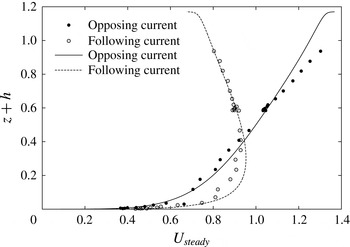
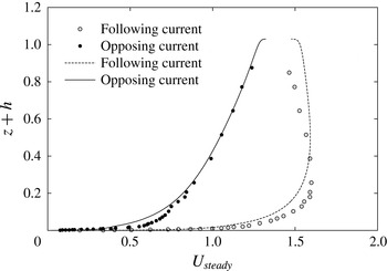
and those measured by Klopman (Reference Klopman1994) for both opposing and following currents. The sign of the steady velocity component has been reversed for the following current case to allow easy evaluation of the results.

Comparison of the steady velocity profiles predicted by the model for
 $h^{\ast }=0.2~\text{m}$
,
 $T=0.9~\text{s}$
,
 $a^{\ast }=0.9~\text{cm}$
and
 $a^{\ast }=0.875~\text{cm}$
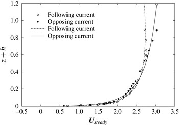
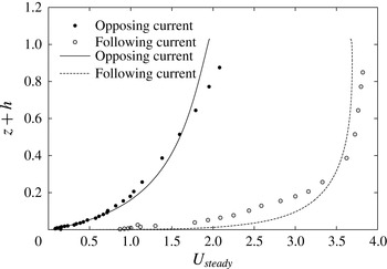
(runs WCA1 and WCF1, respectively) and those measured by Umeyama (Reference Umeyama2005) for both opposing and following currents. The sign of the steady velocity component has been reversed for the following current case to allow easy evaluation of the results.

First, we considered the experiments of Klopman (Reference Klopman1994). Figure 3 shows a comparison between the theoretical results and the measurements of the steady velocity component made by Klopman (Reference Klopman1994) for a monochromatic wave propagating either in the direction of the current or opposite to it. The reader should notice that the waves propagate in the negative
 $x$
direction and, to allow easier evaluation of the results, the steady velocity component in the figures is reversed for the following current case. As indicated by the experimental data, the model shows that the steady velocity near the free surface is increased with respect to the case of a current alone, when the waves propagate in the direction opposite to the direction of the current. On the other hand, the velocity is decreased near the free surface when the waves follow the current. Moreover, the agreement between the model results and the laboratory measurements is not only qualitative but also quantitative, even though small discrepancies are observed mainly close to the free surface for the opposing current case and close to the bottom for the following current case.
A further comparison between theoretical results and experimental measurements is shown in figure 4, where the data by Umeyama (Reference Umeyama2005) are considered. In particular, the figure shows the cases named WCA1 and WCF1 by Umeyama (Reference Umeyama2005), which are for an opposing and a following current, respectively. Also in this case the agreement between the predictions and the experimental data is satisfactory and supports the present analysis.
Since the experiments of Klopman (Reference Klopman1997) were made for a rough bottom but the experiments of Umeyama (Reference Umeyama2005) were made for a smooth bottom, it appears that the model provides reliable predictions for both smooth and rough bottoms.
Comparison of the steady velocity profiles predicted by the model for
 $h^{\ast }=0.2~\text{m}$
,
 $T^{\ast }=1.0~\text{s}$
,
 $a^{\ast }=2.28~\text{cm}$
and
 $a^{\ast }=2.22~\text{cm}$
(runs WDA3 and WCA5, respectively) and those measured by Kemp & Simons (Reference Kemp and Simons1982, Reference Kemp and Simons1983) for both opposing and following currents. The sign of the steady velocity component has been reversed for the following current case to allow easy evaluation of the results.

Comparison of the steady velocity profiles predicted by the model for
 $h^{\ast }=0.2~\text{m}$
,
 $T^{\ast }=1.0~\text{s}$
,
 $a^{\ast }=1.395~\text{cm}$
and
 $a^{\ast }=1.135~\text{cm}$
(runs WDR1 and WCR1, respectively) and those measured by Kemp & Simons (Reference Kemp and Simons1982, Reference Kemp and Simons1983) for both opposing and following currents. The sign of the steady velocity component has been reversed for the following current case to allow easy evaluation of the results.

However, there are experiments which are not well reproduced by the model. To give an example, figure 5 shows a comparison between the model results and the data of Kemp & Simons (Reference Kemp and Simons1982, Reference Kemp and Simons1983) for tests WCA5 and WDA3, which are for a smooth bottom and a following and an opposing current, respectively. In the former case, the agreement is fair even though, close to the bottom, the model slightly underpredicts the steady velocity component. For the opposing wave case, a significant discrepancy can be observed both close to the bottom and in the core region, up to the free surface. Moreover, the maximum value of the steady velocity measured by Kemp & Simons (Reference Kemp and Simons1982) is closer to the bottom than the value predicted by the model. Figure 6 shows a further comparison between the model predictions and the laboratory data of tests WDR1 and WCR1 of Kemp & Simons (Reference Kemp and Simons1982) and Kemp & Simons (Reference Kemp and Simons1983), respectively. In particular, figure 6 shows two cases which are for a following and an opposing current as in figure 5, but for a rough bottom. Discrepancies can be detected in this case too. In the following current case, a significant deviation of the model predictions from the experimental measurements is observed close to the free surface, while in the opposing current case a significant discrepancy appears close to the bottom. However, the qualitative influence of the waves on the current profile is well predicted by the model for all the cases.
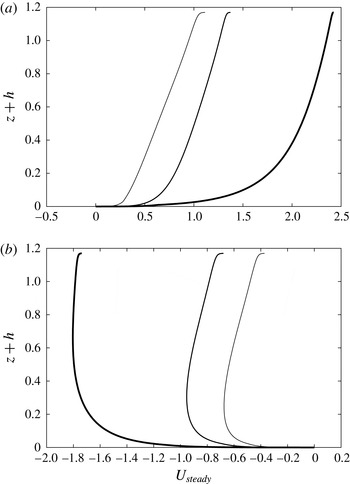
Dimensionless steady velocity component predicted by the model for
 $h^{\ast }=0.5~\text{m}$
,
 $T^{\ast }=1.44~\text{s}$
and
 $a^{\ast }=9~\text{cm}$
(thin line),
 $a^{\ast }=6~\text{cm}$
(intermediate line),
 $a^{\ast }=3~\text{cm}$
(thick line) and both (a) opposing and (b) following current. The dimensional flow rate is kept fixed and equal to that of Klopman’s (Reference Klopman1994) experiments.

At this stage, it is worth pointing out that the Reynolds number
 $R_{{\it\delta}}=U_{0}^{\ast }\sqrt{2}/\sqrt{{\it\omega}^{\ast }{\it\nu}^{\ast }}$
of the oscillatory boundary layer in the experiments is not high – less than
 $100$
for Kemp & Simons’ (Reference Kemp and Simons1982, Reference Kemp and Simons1983) and Umeyama’s (Reference Umeyama2005) experiments – and it might be that the flow relaminarizes during the accelerating phases of the cycle, thus providing a possible justification for the differences between the experimental measurements and the model results obtained by considering a fully turbulent flow.
Altogether, it is possible to conclude that the model provides an acceptable description of the wave–current interaction and it can be used to investigate the influence of the problem parameters on the velocity profile.
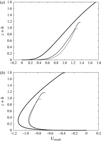
Figure 7 shows the steady velocity profile predicted by the model for values of the parameters equal to those of the experiments of Klopman (Reference Klopman1994) but for different values of the wave amplitude. In particular, the amplitude of the propagating wave is doubled and halved but the dimensional flow rate is kept fixed. This explains why the quantity
 $(\int _{0}^{2{\rm\pi}}\int _{-h}^{0}u\,\text{d}z\,\text{d}{\it\theta})/2$
, which is the dimensionless flow rate, assumes different values. Indeed, the reader should recall that the horizontal velocity component
 $u^{\ast }$
is scaled with
 $a^{\ast }{\it\omega}^{\ast }/S$
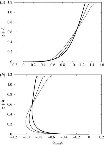
. Figure 8 shows the results for the same parameters as in figure 7 but keeping the dimensionless flow rate fixed.
In both cases, it appears that an increase in the wave amplitude leads to larger values of the velocity near the free surface for an opposing current and to smaller values for a following current. However, this qualitative trend can be recognized more easily when the dimensionless rather than the dimensional flow rate is kept constant.
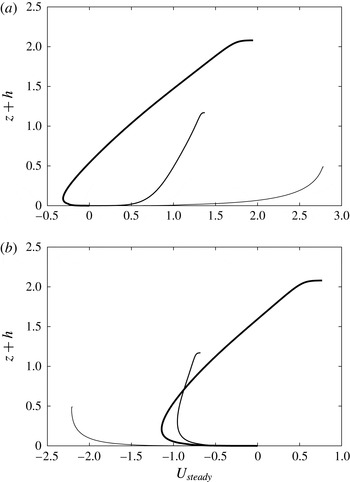
To give an idea of the effects that a variation of the water depth has on the results, figure 9 shows the profile of the horizontal steady velocity component when the value of
 $h^{\ast }$
is 0.375, 0.5 and 0.875 m and the other parameters are kept equal to those characterizing Klopman’s (Reference Klopman1994) experiments but the flow rate is changed to have a constant depth-averaged velocity. Of course, the variation of
 $h^{\ast }$
implies simultaneous variations of the parameters
 $a,h^{\ast }k^{\ast }$
and
 ${\it\delta}_{T}$
. It follows that a direct comparison of the dimensionless results is not straightforward. However, the analysis of figure 9 shows that the interaction between currents and waves is not qualitatively affected by variations of
 $h^{\ast }$
, which have only a quantitative influence on the results.
Dimensionless steady velocity component predicted by the model for
 $h^{\ast }=0.5~\text{m}$
,
 $T^{\ast }=1.44~\text{s}$
and
 $a^{\ast }=9~\text{cm}$
(thin line),
 $a^{\ast }=6~\text{cm}$
(intermediate line),
 $a^{\ast }=3~\text{cm}$
(thick line) and both (a) opposing and (b) following current. The dimensionless flow rate is kept fixed and equal to that of Klopman’s (Reference Klopman1994) experiments.

Dimensionless steady velocity component predicted by the model for
 $T^{\ast }=1.44~\text{s}$
,
 $a^{\ast }=6~\text{cm}$
and
 $h^{\ast }=37.5~\text{cm}$
(thin line),
 $h^{\ast }=50~\text{cm}$
(intermediate line),
 $h^{\ast }=87.5~\text{cm}$
(thick line) and both (a) opposing and (b) following current. For the opposing current, the dimensionless flow rate is equal to
 $0.99$
,
 $1.20$
and
 $1.83$
, respectively, while for the following current it is equal to
 $-0.85$
,
 $-1.01$
and
 $-1.55$
, respectively.

Finally, figure 10 shows the steady velocity profile for different values of the wave period (namely 1.00, 1.44,
 $3.00~\text{s}$
) but with the other parameters kept equal to those of the experiments of Klopman (Reference Klopman1994). Moreover, the dimensionless flow rate is kept fixed. Hence, since an increase of
 $T^{\ast }$
leads to longer waves and smaller values of the dimensionless water depth
 $h$
, the depth-averaged velocity increases and the effects of the waves on the current velocity profile decrease. In particular, for the longest period, the current profile seems only marginally affected by the presence of the waves even though the oscillatory velocity components affect the steady velocity profile, as can be verified by comparing the thin lines of figures 10(a,b).
Dimensionless steady velocity component predicted by the model for
 $h^{\ast }=0.5~\text{m}$
,
 $a^{\ast }=6~\text{cm}$
and
 $T^{\ast }=3.0~\text{s}$
(thin line),
 $T^{\ast }=1.44~\text{s}$
(intermediate line),
 $T^{\ast }=1.0~\text{s}$
(thick line) and both (a) opposing and (b) following current. The dimensionless flow rate is kept fixed and equal to
 $1.19$
for the opposing currents and
 $-1.01$
for the following currents.

As pointed out in § 1, the model can also be easily applied to the study of the interaction between waves and currents when the direction of wave propagation forms an arbitrary angle with the current direction. In this case, to characterize the current, two different independent parameters are needed: either the strength of the current and the angle formed by the direction of the current with the direction of wave propagation, or the depth-averaged values
 $U_{steady}$
and
 $V_{steady}$
of the
 $x$
and
 $y$
components of the steady velocity (
 $U_{steady}=h^{-1}\int _{0}^{h}u\,\text{d}z$
,
 $V_{steady}=h^{-1}\int _{0}^{h}v\,\text{d}z$
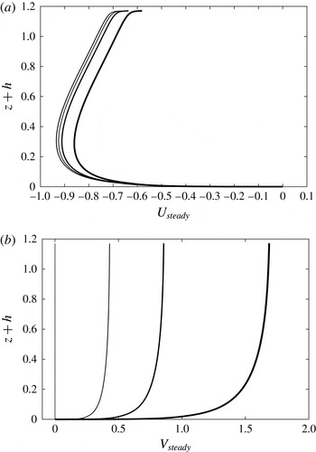
). It follows that an exhaustive investigation of the phenomenon in the parameter space is difficult. Figure 11 shows the steady velocity profile obtained by considering values of the parameters equal to those of Klopman’s (Reference Klopman1994) experiments for the following current case (in particular, the value of the pressure gradient (free surface slope) in the
 $x$
direction is kept fixed) and different values of the pressure gradient in the
 $y$
direction, in order to generate increasing values of the
 $y$
component of the depth-averaged steady velocity component.
The results show that the velocity profile in the transverse direction is close to a logarithmic profile and an increase of
 $V_{steady}$
leads to a small decrease in the
 $x$
component of the depth-averaged steady velocity component
 $U_{steady}$
, even though the velocity profile does not change significantly.
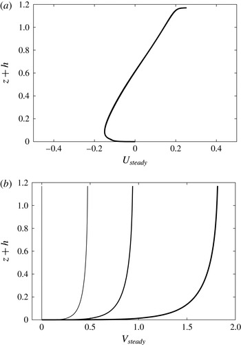
The most interesting case is when the current is orthogonal to the direction of wave propagation, i.e. when the depth-averaged value of the steady velocity component in the direction of wave propagation vanishes.
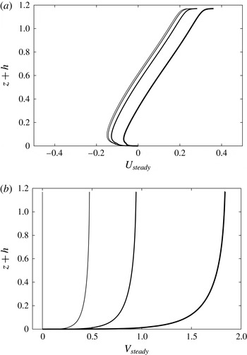
Figure 12 shows the steady velocity profile obtained by considering values of the pressure gradient (free surface slope) along the
 $x$
and
 $y$
directions which generate vanishing values of both
 $U_{steady}$
and
 $V_{steady}$
(see the thinnest lines in figure 12). In the same figure we also plot the velocity profiles obtained by keeping the pressure gradient fixed along the
 $x$
direction and increasing the pressure gradient along the
 $y$
direction. Of course, when the transverse pressure gradient does not vanish, a significant value of
 $V_{steady}$
is observed, which increases for increasing values of
 $\partial \tilde{P}_{0}/\partial y$
. Simultaneously, because of the interaction between the current and the waves, a non-vanishing value of
 $U_{steady}$
is generated, which is not negligible. Indeed, figure 12 shows that an almost constant velocity component in the direction opposite to the direction of wave propagation is generated by an increase in
 $V_{steady}$
.
Of course, vanishing values of
 $U_{steady}$
can be recovered by modifying the streamwise pressure gradient, i.e. the streamwise surface slope, as shown by figure 13. This finding seems to suggest that, in the surf region where the depth- and time-averaged value of the cross-shore velocity should vanish because of the presence of a beach, the interaction between the waves and the longshore current slightly modifies the set-up value, which is determined neglecting this interaction.
Dimensionless steady velocity component predicted by the model for
 $h^{\ast }=0.5~\text{m}$
,
 $a^{\ast }=6~\text{cm}$
,
 $T^{\ast }=1.44~\text{s}$
and different values of the pressure gradient in the transverse
 $y$
direction and a vanishing value of the pressure gradient in the
 $x$
direction. The thinnest line is for a vanishing value of the pressure gradient in the
 $y$
direction and thicker lines are for increasing values, to give rise to
 $V_{steady}=0,0.40,0.80,1.57$
. (a) The
 $x$
component of the velocity; (b) the
 $y$
component.

Dimensionless steady velocity component predicted by the model for
 $h^{\ast }=0.5~\text{m}$
,
 $a^{\ast }=6~\text{cm}$
,
 $T^{\ast }=1.44~\text{s}$
and different values of the pressure gradient in the transverse
 $y$
direction. The pressure gradient in the
 $x$
direction is fixed and equal to the value which generates a vanishing value of
 $U_{steady}$
when there is no steady current in the
 $y$
direction. The thinnest line is for a vanishing value of the pressure gradient in the
 $y$
direction and thicker lines are for increasing values, to give rise to
 $V_{steady}=0,0.44,0.88,1.71$
. (a) The
 $x$
component of the velocity; (b) the
 $y$
component.

Dimensionless steady velocity component predicted by the model for
 $h^{\ast }=0.5~\text{m}$
,
 $a^{\ast }=6~\text{cm}$
,
 $T^{\ast }=1.44~\text{s}$
and different values of the pressure gradient in the transverse
 $y$
direction. The thinnest line is for a vanishing value of the pressure gradient in the
 $y$
direction and thicker lines are for increasing values, to give rise to
 $V_{steady}=0,0.44,0.88,1.71$
. The pressure gradient in the
 $x$
direction is chosen in such a way that
 $U_{steady}$
vanishes. Because of this choice, in (a) the results for different values of the transverse pressure gradient are coincident. (a) The
 $x$
component of the velocity; (b) the
 $y$
component.

5. Concluding remarks
A model is proposed to analyse the effects that wave–current interaction has on the steady velocity profile. The model considers waves of small steepness and mean current velocities of the same order of magnitude as the amplitude of the velocity oscillations induced by wave propagation. Moreover, viscous effects are assumed to be small and mainly confined to the bottom and surface boundary layers. The bottom boundary layer is fully resolved but the boundary layer at the free surface is not considered, since its effect on the current is very weak and can be safely ignored. Moreover, assuming that the parameter
 ${\it\delta}_{T}$
is smaller than the wave steepness, the damping of the wave amplitude is neglected as well.
The model is rather simple and can be easily applied. However, a comparison of the theoretical results with the experimental measurements of different authors supports the validity of the model.
At the leading order of approximation, the interaction between the waves and the current takes place mainly in the bottom boundary layer because of the small values assumed by the ratio between the boundary layer thickness and the length of the wave. At the second order of approximation, the waves modify the mean current profile because of the mean momentum flux induced by the velocity oscillations. As pointed out by Huang & Mei (Reference Huang and Mei2003), it turns out that the mean shear stresses close to the free surface are opposite to the direction of wave propagation. It follows that the mean current is reduced for the following current but increased for the opposing current.
When the current forms an arbitrary angle with the direction of wave propagation, the profile of the velocity component orthogonal to the direction of wave propagation turns out to be close to the logarithmic profile, and the wave–current interaction seems to significantly affect only the velocity component parallel to the direction of wave propagation. In particular, increasing values of
 $V_{steady}$
lead to a reduction of the
 $x$
component of the steady velocity near the free surface. If external conditions force vanishing values of
 $U_{steady}$
, the wave–current interaction turns out to affect the free surface slope.
Acknowledgements
The authors wish to thank Professor Simons, who kindly provided some of the experimental data used to test the predictions of the model. This study was funded by the ‘Ministero dell’Istruzione, dell’Università e della Ricerca’ under research project 2012BYTPR5, ‘Hydro-morphodynamic modelling of coastal processes for engineering purposes’, coordinated by Professor E. Foti (University of Catania) and by the Office of Naval Research (US) under research project N6290914PR00165. Support by the University of Genoa is also acknowledged.