1 Introduction
Vertical mixing in the stably stratified ocean influences the fluxes of heat, carbon, nutrients and other important tracers, and couples with the global overturning circulation (Wunsch & Ferrari Reference Wunsch and Ferrari2004; Kuhlbrodt et al. Reference Kuhlbrodt, Griesel, Montoya, Levermann, Hofmann and Rahmstorf2007). Turbulence and mixing in the stably stratified ocean interior has traditionally been associated with instability of the shear associated with internal waves generated via the action of tides interacting with seafloor bathymetry and winds blowing over the sea surface. Under certain circumstances, such stratified shear flows may be susceptible to a Kelvin–Helmholtz-type instability, leading to a burst of enhanced mixing and dissipation (Garrett Reference Garrett2003; Smyth & Moum Reference Smyth and Moum2012). Regions of turbulence in the ocean are unsteady in time and inhomogeneous in space, leading to difficulties in measuring and quantifying mixing (Ivey, Winters & Koseff Reference Ivey, Winters and Koseff2008).
The Miles–Howard theorem quantifies the stability of parallel inviscid steady shear flows to linear instability via the gradient Richardson number,
 $Ri_{g}=N^{2}/S^{2}$
, which is the ratio between the stabilizing effects of stratification (represented by the buoyancy frequency
 $N$
) and the destabilizing effects of shear (given by
 $S$
, the vertical shear). Flows with
 $Ri_{g}\geqslant 1/4$
everywhere are stable to linear normal-mode perturbations in a steady flow; having
 $Ri_{g}<1/4$
somewhere in the flow is a necessary (though not sufficient) condition for the Kelvin–Helmholtz (KH) instability (Howard Reference Howard1961; Miles Reference Miles1961). In flows which do exhibit instabilities such as the canonical ‘Kelvin–Helmholtz’ instability of inflectional shear layers, typically the initial perturbations grow and saturate, become susceptible to secondary instabilities and eventually break down into small-scale turbulence and mixing via a ‘zoo’ of secondary instabilities (see e.g. Peltier & Caulfield Reference Peltier and Caulfield2003; Mashayek & Peltier Reference Mashayek and Peltier2012). However, it is very important to appreciate that for such free shear layers, the turbulence which arises is inherently transient. Due to the enhanced dissipation associated with the turbulence, these flows inevitably relaminarize eventually, even in the limit as
 $Ri_{g}\rightarrow 0$
unless the shear is reinforced by some external mechanism.
Mixing is an inherently small-scale process, not resolved in large-scale circulation models, and so mixing parameterizations are required. Often, these parameterizations employ a critical Richardson number, below which the effects of turbulence are turned on. For example, a critical value of
 $1/4$
, corresponding to the Miles–Howard stability criterion, is sometimes employed (Mellor & Yamada Reference Mellor and Yamada1982; Price, Weller & Pinkel Reference Price, Weller and Pinkel1986; Kunze, Williams III & Briscoe Reference Kunze, Williams and Briscoe1990). However, the most appropriate choice of this critical value, and indeed whether such a critical value exists at all, is unclear (Polzin Reference Polzin1996). In particular, despite the correlation between enhanced dissipation with low-
 $Ri$
flows, there is observational (Polzin Reference Polzin1996; Mack & Schoeberlein Reference Mack and Schoeberlein2004), experimental (Augier et al.
Reference Augier, Billant, Negretti and Chomaz2014) and numerical evidence (Riley & deBruynKops Reference Riley and deBruynKops2003) indicating that increased dissipation may also be found at higher Richardson numbers. It should be noted that these higher dissipation values are not necessarily in violation of the Miles–Howard theorem, owing to differences between the idealized flow considered in deriving the theorem and the more complicated flows possible in the ocean and laboratory, as well as limitations in measurements. However, they may also suggest that mechanisms other than the classical normal-mode instabilities may be at play in triggering transition to turbulence and mixing in stably stratified fluids.
More recent work has shown that it is possible for disturbances to grow in stratified flows even if the Miles–Howard stability criterion is met and all normal-mode perturbations are stable (Farrell & Ioannou Reference Farrell and Ioannou1993b
; Kaminski, Caulfield & Taylor Reference Kaminski, Caulfield and Taylor2014). Owing to the non-normality of the Navier–Stokes equations, it is possible for perturbations to grow at finite times and then subsequently decay in these ostensibly ‘stable’ flows (Trefethen et al.
Reference Trefethen, Trefethen, Reddy and Driscoll1993; Farrell & Ioannou Reference Farrell and Ioannou1993a
). These ‘optimal perturbations’ (i.e. the perturbations associated with maximum energy growth over some finite time horizon) are able to exploit linear transient growth mechanisms such as the Orr mechanism (Orr Reference Orr1907) and the lift-up mechanism (Ellingsen & Palm Reference Ellingsen and Palm1975) to amplify perturbation amplitude over finite time horizons. Even in flows which admit a normal-mode instability, the perturbation which grows the most at finite times may not be the predicted normal mode (Tearle Reference Tearle2004; Arratia, Caulfield & Chomaz Reference Arratia, Caulfield and Chomaz2013). Farrell & Ioannou (Reference Farrell and Ioannou1993b
), in investigating a uniformly stratified constant shear flow, found that at finite time perturbations were able to grow even for flows stable in the Miles–Howard sense. In fact, though the maximum perturbation growth decreased with increasing stratification, no particular significance was associated with the critical value of
 $Ri=1/4$
. More recently, as reported in Kaminski et al. (Reference Kaminski, Caulfield and Taylor2014), we computed the linear optimal perturbations of a flow with uniform background stratification and hyperbolic tangent shear. We showed that while unstable normal-mode perturbations dominated at long target times, at shorter target times the perturbations leading to maximum growth were not necessarily the normal modes predicted by the Taylor–Goldstein equation. Additionally,
 $O(10{-}100)$
linear perturbation energy gain could be attained even in flows with no predicted unstable normal modes. As we will show here, higher Reynolds numbers can lead to even larger transient growth.
In addition to linear non-normal growth, it is also possible to find nonlinear optimal perturbations for a given base flow. Nonlinear optimal perturbations have been found for a variety of unstratified flows, including plane Couette flow (Rabin, Caulfield & Kerswell Reference Rabin, Caulfield and Kerswell2012; Duguet et al. Reference Duguet, Monokrousos, Brandt and Henningson2013), pipe flow (Pringle & Kerswell Reference Pringle and Kerswell2010) and boundary layers (Cherubini, De Palma & Robinet Reference Cherubini, De Palma and Robinet2015). Recently, nonlinear optimal perturbations have also been identified for stably stratified plane Couette flow, where the presence of stratification is shown to lead to altered structures compared to their unstratified counterparts (Eaves & Caulfield Reference Eaves and Caulfield2015). In general, the structure of the nonlinear optimal perturbations closely matches that of the linear optimal perturbations at small initial amplitude, and becomes increasingly localized in space as the initial perturbation amplitude is increased, until some critical amplitude at which transition to turbulence is able to occur. Nonlinear optimal perturbations have been shown to unpack and grow via a sequence of essentially linear transient growth mechanisms which communicate via nonlinearity as described in Duguet et al. (Reference Duguet, Monokrousos, Brandt and Henningson2013) and Kerswell, Pringle & Willis (Reference Kerswell, Pringle and Willis2014).
In free shear flows at high Reynolds number which are susceptible to primary instabilities of ‘Kelvin–Helmholtz’ type, highly disordered motions with substantially enhanced dissipation are commonly observed to occur due to the development and subsequent break down of secondary instabilities on the primary Kelvin–Helmholtz billow (Caulfield & Peltier Reference Caulfield and Peltier2000). However such a turbulent phase in such flows is inevitably transient, as the enhanced dissipation extracts energy from the background flow, leading to eventual laminarization in the absence of any mechanisms by which the background shear is reinforced. Nevertheless, the onset of such transient turbulence is commonly referred to as ‘transition’ in such flows, and is associated in stratified shear flows at sufficiently high
 $Re$
with the most dynamically significant irreversible mixing of the density field.
Given the substantial linear perturbation growth predicted for finite times, it is natural to question what the fate of these perturbations would be if allowed to evolve in a fully nonlinear fashion. In particular, we are interested in whether the transient growth mechanisms may allow a transition to (inevitably transient) turbulence even when the flow is sufficiently strongly stratified such that the transition is not mediated by the growth of a linear instability. Since the concept of being ‘strongly stratified’ is associated with
 $Ri_{g}$
being sufficiently large everywhere in the flow domain, we shall refer to such a transition as an ‘
 $Ri$
-subcritical transition’, relying as it does on the eventual development of a finite-amplitude perturbation sufficient to trigger transient turbulent motions. It is important to stress that this is not to be confused with the concept of subcritical transition in bounded unstratified shear flows such as pressure-driven flows in pipes or in plane Poiseuille flow, or plane Couette flow between two parallel relatively moving planes, where the ensuing flow is sustained in a statistically steady turbulent state through the continued forcing.
Exploring this key issue of
 $Ri$
-subcritical transition is the central aim of this paper. We find that the degree to which nonlinear effects are important in the evolution of the linear optimal perturbations is increased for higher
 $\mathit{Re}$
, higher initial perturbation amplitude
 $E_{0}$
and lower
 $Ri_{b}$
. In some cases, the perturbations can grow sufficiently large to trigger the onset of secondary instabilities and break down into transient turbulent motions, characterized by markedly enhanced dissipation rates despite the base flow being linearly stable to a primary Kelvin–Helmholtz instability, and so we can indeed observe an
 $Ri$
-subcritical transition to turbulence, in the above-defined sense.
The remainder of the paper is organized as follows. In § 2, we describe the method by which the linear optimal perturbations are computed for a range of Richardson and Reynolds numbers. The resulting linear optimal perturbations for different
 $\mathit{Re}$
are presented in § 3.1. These perturbations are then given finite initial amplitude and used as initial conditions for fully nonlinear direct numerical simulations. A qualitative description of the computed nonlinear flow evolution is presented in § 3.2, and the evolution of mean quantities and turbulent energetics are presented in §§ 3.3 and 3.4, respectively. We discuss our results and draw conclusions in § 4.
2 Formulation
The base flow we consider is a stably stratified shear flow with velocity
 $U^{\ast }(z^{\ast })$
and buoyancy
 $B^{\ast }(z^{\ast })$
given by
 $$\begin{eqnarray}U^{\ast }(z^{\ast })=U_{0}^{\ast }\tanh \left(\frac{z^{\ast }}{h^{\ast }}\right),\quad B^{\ast }(z^{\ast })=N_{0}^{\ast 2}z^{\ast },\end{eqnarray}$$
in which
 $z^{\ast }$
is the vertical coordinate,
 $N_{0}^{\ast }$
is the (uniform) buoyancy frequency, and dimensional quantities are denoted by an asterisk. To non-dimensionalize, we scale lengths by the half-shear-layer width
 $h^{\ast }$
, velocities by
 $U_{0}^{\ast }$
, times by the advective time scale
 $h^{\ast }/U_{0}^{\ast }$
and buoyancy by
 $N_{0}^{\ast 2}h^{\ast }$
. This gives the non-dimensional base flow
 $$\begin{eqnarray}U(z)=\tanh (z),\quad B(z)=z.\end{eqnarray}$$
Using these scales, along with the fluid viscosity
 $\unicode[STIX]{x1D708}^{\ast }$
and (buoyancy) diffusivity
 $\unicode[STIX]{x1D705}^{\ast }$
, three non-dimensional parameters which control the flow evolution can be formed, namely the Reynolds number
 $\mathit{Re}$
, Prandtl number
 $\mathit{Pr}$
and bulk Richardson number
 $Ri_{b}$
, defined as
 $$\begin{eqnarray}\mathit{Re}=\frac{U_{0}^{\ast }h^{\ast }}{\unicode[STIX]{x1D708}^{\ast }},\quad \mathit{Pr}=\frac{\unicode[STIX]{x1D708}^{\ast }}{\unicode[STIX]{x1D705}^{\ast }},\quad Ri_{b}=\frac{N_{0}^{\ast 2}h^{\ast 2}}{U_{0}^{\ast 2}}.\end{eqnarray}$$
For the background flow described by (2.2), the minimum gradient Richardson number occurs at the centre of the shear layer and is equivalent to the value of the bulk Richardson number, i.e.
 $Ri_{g,min}=Ri_{g}(z=0)=Ri_{b}$
. We always choose
 $\mathit{Pr}=1$
for computational simplicity (as higher values of
 $\mathit{Pr}$
require higher resolution of the scalar field).
2.1 Linear optimal perturbations
The behaviour of linear perturbations to the background flow given by (2.2) is described by the Boussinesq Navier–Stokes equations, conservation of buoyancy, and mass continuity linearized about the base flow. In non-dimensional form, the perturbation governing equations are given by
 $$\begin{eqnarray}\displaystyle & \displaystyle \frac{\unicode[STIX]{x2202}u_{i}}{\unicode[STIX]{x2202}t}+u_{j}\frac{\unicode[STIX]{x2202}U_{i}}{\unicode[STIX]{x2202}x_{j}}+U_{j}\frac{\unicode[STIX]{x2202}u_{i}}{\unicode[STIX]{x2202}x_{j}}=-\frac{\unicode[STIX]{x2202}p}{\unicode[STIX]{x2202}x_{i}}+Ri_{b}b\unicode[STIX]{x1D6FF}_{i3}+\frac{1}{\mathit{Re}}\frac{\unicode[STIX]{x2202}^{2}u_{i}}{\unicode[STIX]{x2202}x_{j}\unicode[STIX]{x2202}x_{j}}, & \displaystyle\end{eqnarray}$$
 $$\begin{eqnarray}\displaystyle & \displaystyle \frac{\unicode[STIX]{x2202}b}{\unicode[STIX]{x2202}t}+u_{j}\frac{\unicode[STIX]{x2202}B}{\unicode[STIX]{x2202}x_{j}}+U_{j}\frac{\unicode[STIX]{x2202}b}{\unicode[STIX]{x2202}x_{j}}=\frac{1}{\mathit{Re}\,Pr}\frac{\unicode[STIX]{x2202}^{2}b}{\unicode[STIX]{x2202}x_{j}\unicode[STIX]{x2202}x_{j}}, & \displaystyle\end{eqnarray}$$
 $$\begin{eqnarray}\displaystyle & \displaystyle \frac{\unicode[STIX]{x2202}u_{i}}{\unicode[STIX]{x2202}x_{i}}=0, & \displaystyle\end{eqnarray}$$
where
 $\boldsymbol{u}$
,
 $b$
and
 $p$
are the velocity, buoyancy and pressure perturbations, respectively.
We seek the linear optimal perturbations
 $\boldsymbol{u}_{0}(x,y,z,t)$
and
 $b_{0}(x,y,z,t)$
for the background flow (2.2), i.e. the perturbations which grow the most over a finite time horizon. As described in Kaminski et al. (Reference Kaminski, Caulfield and Taylor2014), the problem may be treated as an optimization problem for total perturbation energy gain,
 $$\begin{eqnarray}G(T)=\frac{{\textstyle \frac{1}{2}}(\langle \boldsymbol{u},\boldsymbol{u}\rangle +Ri_{b}\langle b,b\rangle )}{{\textstyle \frac{1}{2}}(\langle \boldsymbol{u}_{0},\boldsymbol{u}_{0}\rangle +Ri_{b}\langle b_{0},b_{0}\rangle )},\end{eqnarray}$$
over the finite time interval 0 to
 $T$
, in which the angle brackets denote the inner product over the volume,
 $\langle \boldsymbol{f},\boldsymbol{g}\rangle =1/V\int _{V}\boldsymbol{f}\boldsymbol{\cdot }\boldsymbol{g}\,\text{d}V$
. An augmented Lagrangian can be established which constrains perturbation evolution to follow the governing equations, defined as
 $$\begin{eqnarray}\displaystyle {\mathcal{L}} & = & \displaystyle \frac{\langle \boldsymbol{u}(T),\boldsymbol{u}(T)\rangle +Ri_{b}\langle b(T),b(T)\rangle }{\langle \boldsymbol{u}_{0},\boldsymbol{u}_{0}\rangle +Ri_{b}\langle b_{0},b_{0}\rangle }\nonumber\\ \displaystyle & & \displaystyle -\,[\unicode[STIX]{x2202}_{t}u_{i}+u_{j}\unicode[STIX]{x2202}_{j}U_{i}+U_{j}\unicode[STIX]{x2202}_{j}u_{i}+\unicode[STIX]{x2202}_{i}p-Re^{-1}\unicode[STIX]{x2202}_{j}\unicode[STIX]{x2202}_{j}u_{i}-Ri_{b}b\unicode[STIX]{x1D6FF}_{i3},v_{i}]\nonumber\\ \displaystyle & & \displaystyle -\,[\unicode[STIX]{x2202}_{t}b+u_{j}\unicode[STIX]{x2202}_{j}B+U_{j}\unicode[STIX]{x2202}_{j}b-(Re\,Pr)^{-1}\unicode[STIX]{x2202}_{j}\unicode[STIX]{x2202}_{j}b,\unicode[STIX]{x1D711}]-[\unicode[STIX]{x2202}_{i}u_{i},q]\nonumber\\ \displaystyle & & \displaystyle -\,\langle u_{i}(0)-u_{0i},v_{0i}\rangle -\langle b(0)-b_{0},\unicode[STIX]{x1D711}_{0}\rangle .\end{eqnarray}$$
In the above, the square brackets denote the spatio-temporal inner product,
 $[\,\boldsymbol{f},\boldsymbol{g}]=\int _{0}^{T}\langle \boldsymbol{f},\boldsymbol{g}\rangle \,\text{d}t$
. Variations of (2.8) with respect to the forward or ‘direct’ state variables
 $\boldsymbol{u}$
,
 $b$
, and
 $p$
yield the corresponding adjoint equations,
 $$\begin{eqnarray}\displaystyle & \displaystyle \frac{\unicode[STIX]{x2202}v_{i}}{\unicode[STIX]{x2202}t}=v_{j}\frac{\unicode[STIX]{x2202}U_{j}}{\unicode[STIX]{x2202}x_{i}}-\frac{\unicode[STIX]{x2202}}{\unicode[STIX]{x2202}x_{j}}(U_{j}v_{i})+\unicode[STIX]{x1D711}\frac{\unicode[STIX]{x2202}B}{\unicode[STIX]{x2202}x_{i}}-\frac{\unicode[STIX]{x2202}q}{\unicode[STIX]{x2202}x_{i}}-\frac{1}{Re}\frac{\unicode[STIX]{x2202}^{2}v_{i}}{\unicode[STIX]{x2202}x_{j}\unicode[STIX]{x2202}x_{j}}, & \displaystyle\end{eqnarray}$$
 $$\begin{eqnarray}\displaystyle & \displaystyle \frac{\unicode[STIX]{x2202}\unicode[STIX]{x1D711}}{\unicode[STIX]{x2202}t}=-\frac{\unicode[STIX]{x2202}}{\unicode[STIX]{x2202}x_{j}}(U_{j}\unicode[STIX]{x1D711})-Ri_{b}v_{3}-\frac{1}{Re\,Pr}\frac{\unicode[STIX]{x2202}^{2}\unicode[STIX]{x1D711}}{\unicode[STIX]{x2202}x_{j}\unicode[STIX]{x2202}x_{j}}, & \displaystyle\end{eqnarray}$$
 $$\begin{eqnarray}\displaystyle & \displaystyle \frac{\unicode[STIX]{x2202}v_{i}}{\unicode[STIX]{x2202}x_{i}}=0, & \displaystyle\end{eqnarray}$$
which govern the evolution of the adjoint velocity
 $\boldsymbol{v}$
, adjoint buoyancy
 $\unicode[STIX]{x1D711}$
and adjoint pressure
 $q$
, as well as conditions to be satisfied at times
 $t=0$
and
 $t=T$
. The direct or forward equations (2.4)–(2.6) and adjoint equations (2.9)–(2.11) are then used in a direct-adjoint looping (DAL) framework to solve for the linear optimal perturbations (see Kaminski et al. (Reference Kaminski, Caulfield and Taylor2014) for more details of the algorithmic approach).
The flow domain used to compute the linear optimal perturbations has non-dimensional size
 $(L_{x},L_{y},L_{z})=(9.44,15.0,60.0)$
, with a double hyperbolic-tangent shear layer velocity profile and uniform stable background stratification. This corresponds to the base flow described in (2.2), with an additional shear layer of the opposite sign added above in order to impose periodicity for computational convenience (see also (2.2) of Kaminski et al.
Reference Kaminski, Caulfield and Taylor2014). Accordingly, the vertical extent for this calculation is twice that used in the fully nonlinear simulations described below. The two shear layers are sufficiently separated that they may be considered independent. The horizontal extent is chosen to be one wavelength of the most unstable mode predicted by the Taylor–Goldstein equation for
 $Ri_{b}=0.20$
. We choose this extent as our base choice for two reasons. First, consistently with the previous related studies of Tearle (Reference Tearle2004), Arratia et al. (Reference Arratia, Caulfield and Chomaz2013) and Kaminski et al. (Reference Kaminski, Caulfield and Taylor2014), for sufficiently long target times in a flow with a linear instability, the optimal perturbation has the same streamwise extent as the most unstable normal mode. Second, our focus is to determine whether the nonlinear time-dependent evolution arising from linear optimal perturbations can trigger (transient) transition. Therefore, it seems natural for ease of comparison to choose the same streamwise extent as
 $Ri_{b}$
is varied. Additional optimal perturbations are computed with larger horizontal and spanwise extents as shown in appendix A, in order to ascertain the importance of domain size on the computed gain. Particular attention is paid to the optimal perturbations computed for the case with
 $Ri_{b}=0.30$
and the larger horizontal extent
 $(L_{x},L_{y},L_{z})=(12.6,15.0,60.0)$
based on two wavelengths of the perturbation structure identified to have optimal linear gain at this value of
 $Ri_{b}$
as described in Kaminski et al. (Reference Kaminski, Caulfield and Taylor2014).
2.2 Fully nonlinear simulations
Direct numerical simulations are carried out by solving the full nonlinear Boussinesq Navier–Stokes and buoyancy conservation equations. The temporal discretization employs a third-order mixed Runge–Kutta–Wray/Crank–Nicolson scheme, in which the viscous terms are treated semi-implicitly and the advective terms are treated explicitly (as described in Taylor Reference Taylor2008). The horizontal directions are periodic and treated pseudospectrally. In the vertical direction, a second-order finite-difference discretization is used, and the grid points are clustered around the shear layer in the centre of the domain. Sponge layers are used at the top and bottom of the domain to mimic open boundaries.
Linear optimal perturbations are computed as described above, and the structure from the bottom shear layer is subsequently interpolated onto the clustered grid. These perturbations are then given a finite initial amplitude, added onto the background flow (2.2) and used as an initial condition for the direct numerical simulations. Noise with one tenth the initial perturbation amplitude is also added in order to allow for the possible development of secondary instabilities, and is centred on the shear layer with a Gaussian profile in
 $z$
. The noise is white up to a cutoff wavenumber corresponding to the maximum wavenumber of the smallest grid in table 1, so as to use the same noise spectrum across all simulations.
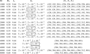
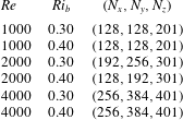
Table 1 gives the details of the simulations considered throughout this paper. The Prandtl number is set to
 $\mathit{Pr}=1$
for all simulations, while
 $\mathit{Re}$
and
 $Ri_{b}$
are varied. The initial perturbation amplitude
 $E_{0}$
(non-dimensionalized by
 $U_{0}^{\ast 2}$
) ranges from
 $5\times 10^{-6}$
to
 $5\times 10^{-5}$
. The grid spacing is determined by the minimum Kolmogorov scale
 $\unicode[STIX]{x1D702}_{min}$
such that
 $\unicode[STIX]{x0394}x_{min}\leqslant 2.1\unicode[STIX]{x1D702}_{min}$
, as suggested by Pope (Reference Pope2000). The domain size is set to
 $(L_{x},L_{y},L_{z})=(9.44,15.0,30.0)$
(except for the case
 $Ri_{b}=0.30$
, in which a domain of size
 $(L_{x},L_{y},L_{z})=(12.6,15.0,30.0)$
is also considered).

3 Results
3.1 Linear optimal perturbations
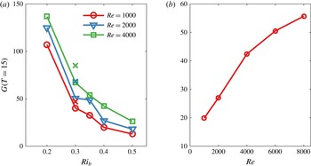
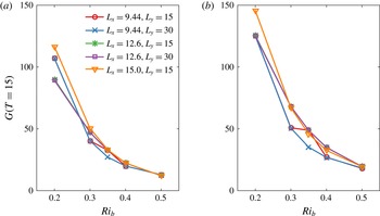
Linear optimal perturbations are computed for
 $Re=1000{-}8000$
,
 $Ri_{b}=0.20$
, 0.30, 0.35, 0.40, 0.50 and
 $Pr=1$
, with a target time of
 $T=15$
, as shown in figure 1. We choose to focus on this particular value of
 $T$
as it is to the target time for which maximum transient growth occurs as shown in Kaminski et al. (Reference Kaminski, Caulfield and Taylor2014). Crucially and conveniently, at this target time, the optimal perturbations are two-dimensional with a horizontal structure corresponding to one or two wavelengths of the domain chosen here. The perturbations take the form of rolls tilted against the background shear which subsequently exploit the Orr mechanism for transient growth as they are tilted upwards over the time interval
 $(0,T)$
(Orr Reference Orr1907). Some of the perturbation energy may be seen in wave-like structures outside of the shear layer for more strongly stratified background flows. The total perturbation energy gain decreases with increasing
 $Ri_{b}$
, as seen by Farrell & Ioannou (Reference Farrell and Ioannou1993a
) and Kaminski et al. (Reference Kaminski, Caulfield and Taylor2014), although
 $O(10^{1}{-}10^{2})$
energy growth is observed even for the flows with no normal-mode instability. In addition, the optimal perturbation gain increases with increasing
 $\mathit{Re}$
; for
 $Ri_{b}=0.40$
, the optimal gain at
 $T=15$
more than doubles between
 $\mathit{Re}=1000$
and
 $\mathit{Re}=4000$
. This is consistent with the optimal gains computed for unstratified shear flows, in which maximum gain increased markedly with
 $\mathit{Re}$
(Arratia et al.
Reference Arratia, Caulfield and Chomaz2013).
Figure 1 also shows that the maximum gain is sensitive to the domain size; the gains corresponding to
 $Ri_{b}=0.30$
in the larger domain (
 $L_{x}=12.6$
) are higher than those for the standard domain (
 $L_{x}=9.44$
). This increase in gain is due to the quantization of the perturbation structure – only discrete wavelengths may fit into the domain, and so the optimal structure (across all streamwise wavenumbers) may be suppressed by the imposed periodicity (associated with the most unstable linear normal mode at
 $Ri_{b}=0.2$
). Thus, it is important to note that there may be structures in different-sized domains that would give somewhat larger (essentially linear) perturbation energy gain compared to the perturbations computed here, although once again we are principally interested in the ensuing inherently nonlinear dynamics. Appendix A shows the result of varying the horizontal and spanwise domain sizes in more detail. However, the fact remains that the transient growth mechanism leads to at least the
 $O(10^{1}{-}10^{2})$
energy gain shown in figure 1, with the possibility of higher growth attainable for different-sized domains.
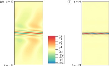
The structure of the linear optimal perturbations for
 $Ri_{b}=0.40$
and
 $\mathit{Re}=1000$
and 4000 is shown in figure 2. The same colour scale is used for both
 $\mathit{Re}$
values for comparison purposes. Both perturbations have the same initial energy, though the energy and corresponding velocity amplitudes themselves are arbitrary as these are linear solutions. While the perturbation in both cases takes the form of rolls tilted against the background shear described above, the lower-
 $\mathit{Re}$
case shows evidence of wave-like structures outside of the shear layer as described in Kaminski et al. (Reference Kaminski, Caulfield and Taylor2014). For the higher-
 $\mathit{Re}$
case, the rolls have a smaller horizontal scale and the wave-like structures are absent. Increasing the Reynolds number changes the structure of the linear optimal perturbation in addition to the maximum gain attained at the target time.
Optimal linear gain for a target time of
 $T=15$
for (a) varying
 $Ri_{b}$
and (b) varying
 $\mathit{Re}$
with
 $Ri_{b}=0.40$
. The
 $\times$
symbols in (a) denote the gains associated with the optimal perturbations with a larger value of
 $L_{x}$
.

Vertical velocity of linear optimal perturbations for
 $Ri_{b}=0.40$
,
 $T=15$
and (a)
 $\mathit{Re}=1000$
and (b)
 $\mathit{Re}=4000$
. The same colour scheme is used for both and the values in (b) saturate the colour bar.

3.2 Nonlinear evolution for
 $\mathit{Re}=4000$
,
$Ri_{b}=0.40$
and
$E_{0}=2\times 10^{-5}$


We now shift our focus to the fully nonlinear results. For the nonlinear simulations, we consider the evolution of the mean quantities, given by the horizontally averaged fields
 $\overline{\boldsymbol{u}}(z,t)$
and
 $\overline{b}(z,t)$
, and the fluctuations away from the mean,
 $\boldsymbol{u}^{\prime }(x,y,z,t)=(u^{\prime },v^{\prime },w^{\prime })$
and
 $b^{\prime }(x,y,z,t)$
. The horizontal average, denoted by an overbar, is defined as
 $$\begin{eqnarray}\overline{f}=\frac{1}{L_{x}}\frac{1}{L_{y}}\int _{0}^{L_{y}}\int _{0}^{L_{x}}f\,\text{d}x\,\text{d}y.\end{eqnarray}$$
If the perturbations evolve entirely linearly, we expect the mean terms to correspond to the background expressions
 $\boldsymbol{U}$
and
 $B$
, defined in (2.2), and the evolution of
 $\boldsymbol{u}^{\prime }$
and
 $b^{\prime }$
to corrspond to the linear optimal perturbations
 $\boldsymbol{u}$
and
 $b$
described above. Conversely, as nonlinear effects become important,
 $\overline{\boldsymbol{u}}$
,
 $\overline{b}$
,
 $\boldsymbol{u}^{\prime }$
and
 $b^{\prime }$
are expected to deviate from their linear counterparts.
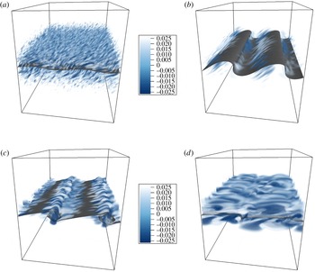
In order to gain a qualitative understanding of how nonlinearity may affect the evolution of the optimal perturbations, figure 3 shows an isosurface of total buoyancy,
 $\overline{b}(z,t)+b^{\prime }(x,y,z,t)$
, at the centre of the shear layer as well as the vertical component of vorticity,
 $\unicode[STIX]{x1D714}_{z}=\unicode[STIX]{x2202}v^{\prime }/\unicode[STIX]{x2202}x-\unicode[STIX]{x2202}u^{\prime }/\unicode[STIX]{x2202}y$
, for
 $\mathit{Re}=4000$
,
 $Ri_{b}=0.40$
and
 $E_{0}=2\times 10^{-5}$
at four times. At early times (figure 3
a), the additive noise obscures the small-amplitude two-dimensional rolls of the optimal perturbation. The rolls are tilted upwards by the mean shear, and if sufficient growth is attained they develop into ‘billows’ (figure 3
b). The billow structure then becomes susceptible to secondary instabilities as highlighted by the oblique structures in vorticity in figure 3(c), and the flow breaks down into small scales which then dissipate and mix the mean flow (figure 3
d). The billows and subsequent break down into turbulence are reminiscent of the nonlinear evolution of the classical Kelvin–Helmholtz instability: formation of two-dimensional billows (e.g. Thorpe Reference Thorpe1973) followed by subsequent onset of secondary instabilities leading to (inherently transient) turbulence onset (e.g. Mashayek & Peltier Reference Mashayek and Peltier2012). However, it should be emphasized that the development of the billows observed in figure 3 arise not due to a classical normal-mode instability as the base flow is linearly stable, but rather through a transient Orr-type growth triggering the development of inherently nonlinear, yet still recognisably billow-like structures.
Evolution of total buoyancy
 $\overline{b}(z,t)+b^{\prime }(x,y,z,t)$
through centre of shear layer (isosurface) and vorticity
 $\unicode[STIX]{x1D714}_{z}=\unicode[STIX]{x2202}v^{\prime }/\unicode[STIX]{x2202}x-\unicode[STIX]{x2202}u^{\prime }/\unicode[STIX]{x2202}y$
(colour) for
 $\mathit{Re}=4000$
,
 $Ri_{b}=0.40$
and
 $E_{0}=2\times 10^{-5}$
. Snapshots of the flow are shown at (a)
 $t=6.0$
, (b)
 $t=12.2$
, (c)
 $t=24.4$
and (d)
 $t=36.7$
. The region shown is
 $z=-2.5$
to
 $z=2.5$
and the aspect ratio has been stretched by a factor of two in the vertical to highlight the detail of the evolving flow.

3.3 Evolution of mean quantities
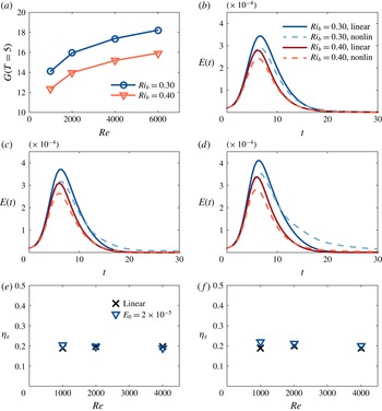
We now consider the total perturbation energy evolution,
 $$\begin{eqnarray}E(t)=\frac{\langle \boldsymbol{u}^{\prime }(t),\boldsymbol{u}^{\prime }(t)\rangle +Ri_{b}\langle b^{\prime }(t),b^{\prime }(t)\rangle }{2},\end{eqnarray}$$
with respect to time, where the angle brackets denote the same inner product as in (2.7). Figure 4 shows the fully nonlinear perturbation energy evolution as well as corresponding energy evolution for a perturbation with the same initial amplitude evolving in an entirely linear manner (as in the computation of the linear optimal perturbations, described above). The simulations shown in figure 4 have
 $Ri_{b}=0.30$
,
 $L_{x}=12.6$
, corresponding to perturbations which experience large gain on a base flow which is relatively close to the Miles–Howard criterion, and
 $Ri_{b}=0.40$
,
 $L_{x}=9.44$
, corresponding to perturbations growing on a more strongly stratified base flow. The initial perturbation amplitude is
 $E_{0}=2\times 10^{-5}$
, and a range of Reynolds numbers,
 $\mathit{Re}=1000$
, 2000 and 4000 are shown. These parameters are chosen in order to highlight a range of different behaviours across the various simulations described in table 1.
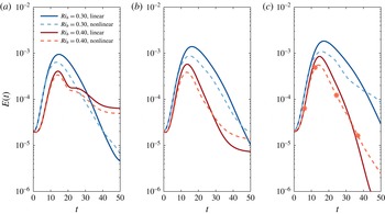
The higher gains predicted by figure 1 can be seen in the energy evolution shown in figure 4. In general, the nonlinear flow evolution begins with a decrease in perturbation amplitude as the additive noise decays. This is followed by a period of linear perturbation energy growth, in which the perturbations extract energy from the background shear flow via the stratified Orr mechanism, as described by Kaminski et al. (Reference Kaminski, Caulfield and Taylor2014). Eventually, nonlinear effects become important and the nonlinear perturbation energy saturates, reaching a lower peak amplitude than the purely linear energy evolution. The energy decays at later times in both the linear and nonlinear cases.
In general, the cases with lower initial amplitude
 $E_{0}$
, lower
 $\mathit{Re}$
and higher
 $Ri_{b}$
more closely follow the linear flow evolution of the computed optimal perturbations. Conversely, cases with higher
 $E_{0}$
, higher
 $\mathit{Re}$
and lower
 $Ri_{b}$
generally show a more dramatic deviation from the linear case, with nonlinear saturation happening earlier in the flow evolution. The comparison between the linear and nonlinear energy evolution indicates when nonlinear effects start to become important, both in terms of initial amplitude and time. It should be emphasized that even in cases in which nonlinear saturation is significant (e.g. figure 4
c), this saturation only occurs after an extended period of quasi-linear perturbation growth, indicating that it is the linear growth mechanism leading to the growth in perturbation energy, rather than some nonlinear response to a large perturbation.


We can examine further the evolution of the optimal perturbation and the subsequent secondary instabilities by considering different components of the perturbation energy. For instance, we can consider the relative contributions of two-dimensional (spanwise-averaged) motions, associated with the optimal perturbations, and of inherently three-dimensional motions, associated with the observed secondary instabilities and subsequent small-scale features which arise. By writing the fluctuation velocity and buoyancy as
 $$\begin{eqnarray}\boldsymbol{u}^{\prime }=\boldsymbol{u}_{2D}^{\prime }+\boldsymbol{u}_{3D}^{\prime }\quad \text{and}\quad b^{\prime }=b_{2D}^{\prime }+b_{3D}^{\prime },\end{eqnarray}$$
where
 $\boldsymbol{u}_{2D}^{\prime }=1/L_{y}\int _{0}^{L_{y}}\boldsymbol{u}^{\prime }\,\text{d}y$
and
 $b_{2D}^{\prime }=1/L_{y}\int _{0}^{L_{y}}b^{\prime }\,\text{d}y$
, we can then define
 $$\begin{eqnarray}E_{2D}=\frac{\langle \boldsymbol{u}_{2D}^{\prime },\boldsymbol{u}_{2D}^{\prime }\rangle +Ri_{b}\langle b_{2D}^{\prime },b_{2D}^{\prime }\rangle }{2}\quad \text{and}\quad E_{3D}=\frac{\langle \boldsymbol{u}_{3D}^{\prime },\boldsymbol{u}_{3D}^{\prime }\rangle +Ri_{b}\langle b_{3D}^{\prime },b_{3D}^{\prime }\rangle }{2}\end{eqnarray}$$
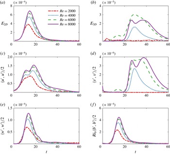
as the energy contributions from two- and three-dimensional motions, respectively. Figure 5(a,b) shows the time evolution of
 $E_{2D}$
and
 $E_{3D}$
for the cases with
 $Ri_{b}=0.40$
,
 $E_{0}=2\times 10^{-5}$
and
 $\mathit{Re}=2000$
–8000. In the case of
 $\mathit{Re}=2000$
, almost all of the perturbation energy is contained in the two-dimensional motions. However, for higher values of
 $\mathit{Re}$
, there is a clear onset of three-dimensional motion beginning at times around
 $t\sim 20$
, when the secondary instabilities themselves onset (as seen qualitatively in figure 3
b).
The observed three-dimensionalization of the flow is further supported by decomposing the fluctuation energy budget into terms corresponding to the streamwise, spanwise and vertical velocities, as well as the buoyancy, i.e.
 $$\begin{eqnarray}E=\frac{\langle \boldsymbol{u}^{\prime },\boldsymbol{u}^{\prime }\rangle +Ri_{b}\langle b^{\prime },b^{\prime }\rangle }{2}=\frac{\langle u^{\prime },u^{\prime }\rangle }{2}+\frac{\langle v^{\prime },v^{\prime }\rangle }{2}+\frac{\langle w^{\prime },w^{\prime }\rangle }{2}+\frac{Ri_{b}\langle b^{\prime },b^{\prime }\rangle }{2}.\end{eqnarray}$$
Figure 5(c–f) shows the contribution of each of these components to the overall energy evolution. It is clear that as
 $E_{3D}$
increases, so does the component owing to the spanwise fluctuation velocity for
 $\mathit{Re}\geqslant 4000$
– the flow is becoming increasingly three-dimensional both in spatial structure and in velocity component. This three-dimensionalization of the flow has been identified as an important step in the transition process for stratified shear flows (Caulfield & Peltier Reference Caulfield and Peltier2000).
Perturbation energy by component for
 $Ri_{b}=0.40$
,
 $E_{0}=2\times 10^{-5}$
and varying
 $\mathit{Re}$
. (a) Two-dimensional component of energy,
 $E_{2D}(t)$
. (b) Three-dimensional component of energy,
 $E_{3D}(t)$
. (c) Streamwise velocity component,
 $\langle u^{\prime },u^{\prime }\rangle /2$
. (d) Spanwise velocity component,
 $\langle v^{\prime },v^{\prime }\rangle /2$
. (e) Vertical velocity component,
 $\langle w^{\prime },w^{\prime }\rangle /2$
. (f) Potential energy component,
 $Ri_{b}\langle b^{\prime },b^{\prime }\rangle /2$
.

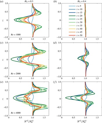
Figure 6 shows the evolution of the mean squared buoyancy frequency, defined as
 $$\begin{eqnarray}\frac{N^{\ast 2}}{N_{0}^{\ast 2}}=\frac{\unicode[STIX]{x2202}\overline{b}}{\unicode[STIX]{x2202}z},\end{eqnarray}$$
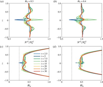
in the vicinity of the shear layer at a series of times over the course of the flow evolution. The cases shown correspond to the same nonlinear simulations as those shown in figure 4. For
 $\mathit{Re}=1000$
and
 $Ri_{b}=0.40$
(figure 6
b), there is very little modification of the background stratification, consistent with the energy evolution shown in figure 4(a): the linear and nonlinear simulations evolve very similarly, indicating that the perturbation evolution in this case is primarily linear. Thus, little modification of the mean flow would be expected in this case, as observed.
For all other cases shown in figure 6, the evolution of the mean stratification shows the signature of localized mixing. A layer of decreased stratification is surrounded by layers of enhanced stratification. The layered structure is similar to that resulting from classical Kelvin–Helmholtz instability (Klaassen & Peltier Reference Klaassen and Peltier1985; Smyth, Moum & Caldwell Reference Smyth, Moum and Caldwell2001; Salehipour, Caulfield & Peltier Reference Salehipour, Caulfield and Peltier2016). The layer structure is strongest at
 $t=15{-}25$
(at which time the flow has noticeably deviated from the linear evolution in figure 4), after which further flow evolution and diffusion act to remove the layer structure and return the mean flow to its initial uniform stratification. For
 $\mathit{Re}=1000$
and
 $Ri_{b}=0.30$
(figure 6
a) and for
 $\mathit{Re}=2000$
and
 $Ri_{b}=0.40$
(figure 6
d), the mean stratification evolves smoothly and is relatively symmetric in the vertical at later times. For the higher-
 $\mathit{Re}$
flows shown in figure 6(c,e,f), not only is the layering much more pronounced, but the structure of the mean stratification becomes much more complicated at later times as a result of the more vigorous secondary instabilities seen in these flows.
Time evolution of scaled mean buoyancy frequency,
 $N^{\ast 2}/N_{0}^{\ast 2}=\unicode[STIX]{x2202}\overline{b}/\unicode[STIX]{x2202}z$
, in the vertical region centred on the shear layer. (a,c,e) Corresponds to
 $Ri_{b}=0.30$
and (b,d,f) corresponds to
 $Ri_{b}=0.40$
. (a,b)
 $\mathit{Re}=1000$
. (c,d)
 $\mathit{Re}=2000$
. (e,f)
 $\mathit{Re}=4000$
. Note that
 $E_{0}=2\times 10^{-5}$
for all cases shown here.

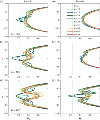
Next, we examine the mean gradient Richardson number of the flow, defined as
 $$\begin{eqnarray}Ri_{g}=\frac{\unicode[STIX]{x2202}\overline{b}/\unicode[STIX]{x2202}z}{(\unicode[STIX]{x2202}\overline{u}/\unicode[STIX]{x2202}z)^{2}},\end{eqnarray}$$
where the overbar denotes the horizontal average used in (3.1). While the local gradient Richardson number,
 $N^{2}/S^{2}$
, varies spatially, this mean quantity gives an overall picture of the stability of the shear layer as the initial perturbation evolves. Figure 7 shows the evolution of the mean gradient Richardson number around the centre of the shear layer for the same simulations as considered in figures 4 and 6.
In the
 $\mathit{Re}=1000$
,
 $Ri_{b}=0.40$
case, where very little modification of the background stratification was observed, the mean gradient Richardson number gradually increases as the mean flow diffuses outwards. In all other cases the evolution of the mean gradient Richardson number is more complicated. This is particularly true for the higher-
 $\mathit{Re}$
cases in which more vigorous secondary instabilities lead to
 $Ri_{g}$
profiles of increasing complexity at later times. Of note are the local minima observed at the centres of the shear layers. These minima approximately coincide with the time of strongest layering in figure 6,
 $t\sim 15{-}20$
, and in most cases fall well below the classical Miles–Howard ‘critical’ value of
 $1/4$
– even in the case
 $Ri_{b}=0.40$
and
 $\mathit{Re}=4000$
(figure 7
f). That is, the nonlinear evolution of the non-normal modes is able to drive the flow towards a mean state which may be unstable in a normal-mode sense, despite starting from an initial background state which is linearly stable.
Evolution of mean gradient Richardson number (defined by (3.7)), in region around shear layer. (a,c,e) Corresponds to
 $Ri_{b}=0.30$
and (b,d,f) corresponds to
 $Ri_{b}=0.40$
. The dotted line denotes
 $Ri_{g}=0.25$
. (a,b)
 $\mathit{Re}=1000$
. (c,d)
 $\mathit{Re}=2000$
. (e,f)
 $\mathit{Re}=4000$
. Note that
 $E_{0}=2\times 10^{-5}$
for all cases shown here.

3.4 Turbulent energetics and mixing
In the previous subsection, we observed that linear transient growth may lead to a large increase in the perturbation energy. Subsequently, departure from the linear evolution may be observed, and the resulting nonlinear effects modify the mean density and
 $Ri_{g}$
profiles. In this section, we will examine the details of the turbulent energetics and mixing in greater detail.
We construct energy budgets for the perturbation kinetic energy
 $k=u_{j}^{\prime }u_{j}^{\prime }/2$
and potential energy
 $\unicode[STIX]{x1D719}=Ri_{b}b^{\prime 2}/2$
from the equations governing conservation of momentum and buoyancy. Applying the same average as in (3.1), the horizontally averaged perturbation kinetic and potential energy budgets are given by
 $$\begin{eqnarray}\displaystyle \frac{\unicode[STIX]{x2202}\overline{k}}{\unicode[STIX]{x2202}t}=-\underbrace{\frac{\unicode[STIX]{x2202}\overline{p^{\prime }w^{\prime }}}{\unicode[STIX]{x2202}z}}_{\text{pressure transp.}}-\underbrace{\frac{\unicode[STIX]{x2202}\overline{kw^{\prime }}}{\unicode[STIX]{x2202}z}}_{\text{turbulent transp.}}+\underbrace{Ri_{b}\overline{b^{\prime }w^{\prime }}}_{\text{buoyancy flux}}-\underbrace{\overline{u^{\prime }w^{\prime }}\frac{\unicode[STIX]{x2202}\overline{u}}{\unicode[STIX]{x2202}z}}_{\text{shear prod.}}+\underbrace{\frac{1}{\mathit{Re}}\frac{\unicode[STIX]{x2202}^{2}\overline{k}}{\unicode[STIX]{x2202}z^{2}}}_{\text{viscous transp.}}-\underbrace{\unicode[STIX]{x1D700}_{k}}_{\text{KE diss.}},\end{eqnarray}$$
and
 $$\begin{eqnarray}\frac{\unicode[STIX]{x2202}\overline{\unicode[STIX]{x1D719}}}{\unicode[STIX]{x2202}t}=-\underbrace{\frac{\unicode[STIX]{x2202}\overline{\unicode[STIX]{x1D719}w^{\prime }}}{\unicode[STIX]{x2202}z}}_{\text{turbulent transp.}}-\underbrace{Ri_{b}\overline{b^{\prime }w^{\prime }}\frac{\unicode[STIX]{x2202}\overline{b}}{\unicode[STIX]{x2202}z}}_{\text{buoyancy flux}}+\underbrace{\frac{1}{\mathit{Re}\mathit{Pr}}\frac{\unicode[STIX]{x2202}^{2}\overline{\unicode[STIX]{x1D719}}}{\unicode[STIX]{x2202}z^{2}}}_{\text{diffusive transp.}}-\underbrace{\unicode[STIX]{x1D700}_{p}}_{\text{PE diss.}},\end{eqnarray}$$
respectively. The strictly positive terms
 $\unicode[STIX]{x1D700}_{k}$
and
 $\unicode[STIX]{x1D700}_{p}$
represent sinks of perturbation kinetic energy via viscous dissipation and perturbation potential energy via diffusion, respectively and are defined as
 $$\begin{eqnarray}\unicode[STIX]{x1D700}_{k}=\frac{1}{\mathit{Re}}\overline{\frac{\unicode[STIX]{x2202}u_{i}^{\prime }}{\unicode[STIX]{x2202}x_{j}}\frac{\unicode[STIX]{x2202}u_{i}^{\prime }}{\unicode[STIX]{x2202}x_{j}}}\quad \text{and}\quad \unicode[STIX]{x1D700}_{p}=\frac{Ri_{b}}{\mathit{Re}\,\mathit{Pr}}\overline{\frac{\unicode[STIX]{x2202}b^{\prime }}{\unicode[STIX]{x2202}x_{j}}\frac{\unicode[STIX]{x2202}b^{\prime }}{\unicode[STIX]{x2202}x_{j}}}.\end{eqnarray}$$
The shear production term,
 $-\overline{u^{\prime }w^{\prime }}\,\unicode[STIX]{x2202}\overline{u}/\unicode[STIX]{x2202}z$
, describes the interaction between the perturbation kinetic energy and the mean shear, while the vertical buoyancy flux terms
 $Ri_{b}\overline{b^{\prime }w^{\prime }}$
and
 $Ri_{b}\overline{b^{\prime }w^{\prime }}\,\unicode[STIX]{x2202}\overline{b}/\unicode[STIX]{x2202}z$
describe the conversion between kinetic and potential energy as well as interaction with the mean stratification. The remaining terms describe turbulent transport of kinetic and potential energy within the domain (
 $\unicode[STIX]{x2202}\overline{kw^{\prime }}/\unicode[STIX]{x2202}z$
and
 $\unicode[STIX]{x2202}\overline{\unicode[STIX]{x1D719}w^{\prime }}/\unicode[STIX]{x2202}z$
), viscous and diffusive transport (
 $1/\mathit{Re}\,\unicode[STIX]{x2202}^{2}\overline{k}/\unicode[STIX]{x2202}z^{2}$
and
 $Ri_{b}/\mathit{Re}\,\mathit{Pr}\,\unicode[STIX]{x2202}^{2}\overline{\unicode[STIX]{x1D719}}/\unicode[STIX]{x2202}z^{2}$
) and pressure transport (
 $\unicode[STIX]{x2202}\overline{p^{\prime }w^{\prime }}/\unicode[STIX]{x2202}z$
).
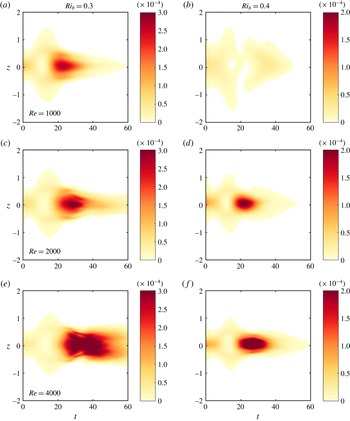
The evolution of the horizontally averaged turbulent dissipation,
 $\unicode[STIX]{x1D700}_{k}$
, is shown as a function of time
 $t$
and the vertical coordinate
 $z$
in figure 8. The simulations shown correspond to those from figure 4. After a short initial period in which the added noise perturbation decays (
 $t\sim 0{-}5$
), the dissipation is fairly low and slightly offset from the centre of the shear layer, corresponding to the edges of the rolls as they are tilted upward by the mean shear. As the rolls lead to the billow structure and smaller-scale secondary instabilities onset, a period of significantly enhanced dissipation is observed in most cases (corresponding to those which exhibited strong nonlinear effects in figures 6 and 7). This enhanced dissipation is confined to a narrow region around the centre of the shear layer. The observed dissipation decreases with increasing
 $Ri_{b}$
, and increases with increasing
 $\mathit{Re}$
, as might be expected based on the increasingly complex structure observed for e.g. figure 6(e,f), indicative of vigorous small-scale structures that would lead to higher dissipation. Also in accordance with figures 6 and 7, in the case of
 $Ri_{b}=0.40$
and
 $\mathit{Re}=1000$
(figure 8
b),
 $\unicode[STIX]{x1D700}_{k}$
remains low as the flow remains quasi-linear throughout the evolution of the perturbations.


In order to assess the relative importance of the various terms in the perturbation energy budgets throughout the domain, we can integrate (3.8) and (3.9) in a control volume defined by the vertical extents
 $z_{1}$
and
 $z_{2}$
. The kinetic and potential energy budgets then become
 $$\begin{eqnarray}\frac{\unicode[STIX]{x2202}}{\unicode[STIX]{x2202}t}\int _{z_{1}}^{z_{2}}\overline{k}\,\text{d}z=\left[-\overline{kw^{\prime }}-\overline{p^{\prime }w^{\prime }}-\frac{1}{\mathit{Re}}\frac{\unicode[STIX]{x2202}\overline{k}}{\unicode[STIX]{x2202}z}\right]_{z_{1}}^{z_{2}}+\int _{z_{1}}^{z_{2}}\left(Ri_{b}\overline{b^{\prime }w^{\prime }}-\overline{u^{\prime }w^{\prime }}\frac{\unicode[STIX]{x2202}\overline{u}}{\unicode[STIX]{x2202}z}-\unicode[STIX]{x1D700}_{k}\right)\text{d}z\end{eqnarray}$$
and
 $$\begin{eqnarray}\frac{\unicode[STIX]{x2202}}{\unicode[STIX]{x2202}t}\int _{z_{1}}^{z_{2}}\overline{\unicode[STIX]{x1D719}}\,\text{d}z=\left[-\overline{\unicode[STIX]{x1D719}w^{\prime }}-\frac{1}{\mathit{Re}\mathit{Pr}}\frac{\unicode[STIX]{x2202}\overline{\unicode[STIX]{x1D719}}}{\unicode[STIX]{x2202}z}\right]_{z_{1}}^{z_{2}}+\int _{z_{1}}^{z_{2}}\left(-Ri_{b}\overline{b^{\prime }w^{\prime }}\frac{\unicode[STIX]{x2202}\overline{b}}{\unicode[STIX]{x2202}z}-\unicode[STIX]{x1D700}_{p}\right)\text{d}z\end{eqnarray}$$
respectively. For a control volume with vertical extents outside of the shear layer, we might expect that the shear production, buoyancy flux terms and sinks owing to dissipation are important, as in the purely linear case (Kaminski et al. Reference Kaminski, Caulfield and Taylor2014), and that the energy flux associated with the viscous and advective transport terms would be small. The pressure transport term may be important if waves are generated during the flow evolution.
In order to assess the relative importance of the two sinks
 $\unicode[STIX]{x1D700}_{k}$
and
 $\unicode[STIX]{x1D700}_{p}$
, we consider a control volume with boundaries at
 $z_{1}=-6$
and
 $z_{2}=6$
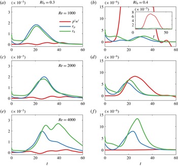
. As figure 8 shows, these vertical extents are well separated from the region of high dissipation occurring near the centre of the shear layer. The results presented here are relatively insensitive to the vertical extent of the control volume provided the boundaries are away from the shear layer and evolving perturbation. Figure 9 shows the evolution of integrated dissipation in the control volume as a function of time for the
 $E_{0}=2\times 10^{-5}$
, as in the previous figures. In general, as
 $\mathit{Re}$
increases, the total dissipation of both kinetic and potential energy in the control volume reaches a higher maximum value. For
 $Ri_{b}=0.30$
and
 $\mathit{Re}=1000$
and 2000 (figure 9
a,c), the peak values in dissipation of kinetic and potential energy occur at approximately the same time, and have approximately the same magnitude. However, at the higher Reynolds number
 $\mathit{Re}=4000$
, shown in figure 9(e), the kinetic energy dissipation reaches a larger maximum value and remains elevated for a much longer period of time than the potential energy dissipation, suggesting that ‘mixing’ of potential energy and dissipation of kinetic energy are not necessarily well time correlated (see e.g. Mashayek, Caulfield & Peltier Reference Mashayek, Caulfield and Peltier2013). A similar trend can be seen when comparing the dissipation rates for
 $Ri_{b}=0.40$
(figure 9
b,d,e): as
 $\mathit{Re}$
increases, the kinetic energy dissipation increases relative to the potential energy dissipation. In the specific case of
 $Ri_{b}=0.40$
and
 $\mathit{Re}=1000$
, for which the flow evolution is quasi-linear (as shown in figures 6 and 7), the amount of dissipation in the control volume is quite low in comparison to the other cases shown in figure 9. In all cases, the peak values of
 $\unicode[STIX]{x1D700}_{k}$
and
 $\unicode[STIX]{x1D700}_{p}$
occur after nonlinear effects have become important in the flow, as discussed in the previous section.
In addition to dissipation of kinetic and potential energy via viscosity and diffusion, energy may also leave the control volume through the effect of internal waves. Given the internal waves observed for the linear scenario in Kaminski et al. (Reference Kaminski, Caulfield and Taylor2014), it is natural to question how significant the transport of energy by waves is when compared with the dissipative terms. We quantify the flux of energy through the edges of the control volume by the pressure transport
 $\overline{p^{\prime }w^{\prime }}|_{z_{1}}^{z_{2}}$
. Away from the shear layer, where the flow is stratified and quasi-linear, we expect the effects of internal waves to dominate the pressure transport. We plot
 $\overline{p^{\prime }w^{\prime }}|_{z_{1}}^{z_{2}}$
as a function of time in figure 9 in order to quantify the importance of the flux via waves relative to the dissipative sink terms.
For
 $Ri_{b}=0.30$
(figure 9
a,c,e),
 $\overline{p^{\prime }w^{\prime }}|_{z_{1}}^{z_{2}}$
is significantly lower than that of the sinks
 $\int _{z_{1}}^{z_{2}}\unicode[STIX]{x1D700}_{k}\,\text{d}z$
and
 $\int _{z_{1}}^{z_{2}}\unicode[STIX]{x1D700}_{p}\,\text{d}z$
, and arises from the localized evolution of the perturbation in the shear layer rather than from internal waves propagating away from the centre of the domain. However, when
 $Ri_{b}=0.40$
, the role of internal waves is potentially very different. While the dissipative terms are still the dominant terms when
 $Ri_{b}=0.40$
and
 $\mathit{Re}=4000$
(figure 9
f), similarly to the cases with
 $Ri_{b}=0.30$
, for
 $\mathit{Re}=2000$
(figure 9
d) the magnitude of the wave flux term is comparable to and in fact slightly larger than the peak values in the dissipative terms, and for
 $\mathit{Re}=1000$
(the nearly linear case discussed above (figure 9
b)) the flux of energy via internal waves is much larger than the dissipation of both kinetic and potential energy. In general, there is a shift from an internal wave-dominated regime to one in which turbulent dissipation is dominant as
 $\mathit{Re}$
increases and
 $Ri_{b}$
decreases.
Evolution of
 $\int _{z_{1}}^{z_{2}}\unicode[STIX]{x1D700}_{k}\,\text{d}z$
,
 $\int _{z_{1}}^{z_{2}}\unicode[STIX]{x1D700}_{p}\,\text{d}z$
and
 $\overline{p^{\prime }w^{\prime }}|_{z_{1}}^{z_{2}}$
, where
 $z_{1}$
and
 $z_{2}$
correspond to the control volume shown in figure 8, as a function of time. The simulations are the same as those in figures 6 and 7.

As seen in figure 5, for higher-
 $\mathit{Re}$
flows there is a clear three-dimensionalization of the flow as secondary instabilities set in on the primarily two-dimensional optimal perturbation. In order to assess the energetics corresponding to these three-dimensional structures, we construct spectral energy budgets from the nonlinear perturbation governing equations (as with the spatial energy budgets (3.8) and (3.9), above). We first Fourier transform the governing equations in the
 $x$
and
 $y$
directions, denoting transformed variables with a caret. Then, by multiplying the governing equations by the complex conjugates of velocity and buoyancy (denoted here by an asterisk), we obtain the spectral form of the kinetic energy budget,
 $$\begin{eqnarray}\frac{\unicode[STIX]{x2202}}{\unicode[STIX]{x2202}t}\text{Re}\left[\frac{\hat{\boldsymbol{u}}^{\prime \ast }\boldsymbol{\cdot }\hat{\boldsymbol{u}}^{\prime }}{2}\right]=\text{Re}\left[-\hat{\boldsymbol{u}}^{\prime \ast }\boldsymbol{\cdot }(\widehat{\boldsymbol{u}^{\prime }\boldsymbol{\cdot }\unicode[STIX]{x1D735}\boldsymbol{u}^{\prime }})-\hat{u} ^{\prime \ast }{\hat{w}}^{\prime }\frac{\unicode[STIX]{x2202}\overline{u}}{\unicode[STIX]{x2202}z}-\hat{\boldsymbol{u}}^{\prime \ast }\boldsymbol{\cdot }\widehat{\unicode[STIX]{x1D735}p}+Ri_{b}{\hat{w}}^{\prime \ast }\hat{b}^{\prime }+\frac{\hat{\boldsymbol{u}}^{\prime \ast }\boldsymbol{\cdot }\widehat{\unicode[STIX]{x1D6FB}^{2}\boldsymbol{u}^{\prime }}}{\mathit{Re}}\right],\end{eqnarray}$$
and the spectral form of the potential energy budget,
 $$\begin{eqnarray}\frac{\unicode[STIX]{x2202}}{\unicode[STIX]{x2202}t}\text{Re}\left[\frac{Ri_{b}\hat{b}^{\prime \ast }\cdot \hat{b}^{\prime }}{2}\right]=\text{Re}\left[-Ri_{b}\hat{b}^{\prime \ast }(\widehat{\boldsymbol{u}^{\prime }\boldsymbol{\cdot }\unicode[STIX]{x1D735}b^{\prime }})-Ri_{b}\hat{b}^{\prime \ast }{\hat{w}}^{\prime }\frac{\unicode[STIX]{x2202}\overline{b}}{\unicode[STIX]{x2202}z}+\frac{Ri_{b}\hat{b}^{\prime \ast }\cdot \widehat{\unicode[STIX]{x1D6FB}^{2}b^{\prime }}}{\mathit{Re}\,\mathit{Pr}}\right].\end{eqnarray}$$
Equations (3.13) and (3.14) allow us to examine the evolution of specific length scales in the flow. We define
 $$\begin{eqnarray}{\mathcal{P}}_{low}=\iint _{|\boldsymbol{k}|<k_{c}}\left(-\hat{u} ^{\prime \ast }{\hat{w}}^{\prime }\frac{\unicode[STIX]{x2202}\overline{u}}{\unicode[STIX]{x2202}z}\right)\text{d}k_{x}\,\text{d}k_{y},\quad {\mathcal{P}}_{high}=\iint _{|\boldsymbol{k}|>k_{c}}\left(-\hat{u} ^{\prime \ast }{\hat{w}}^{\prime }\frac{\unicode[STIX]{x2202}\overline{u}}{\unicode[STIX]{x2202}z}\right)\text{d}k_{x}\,\text{d}k_{y}\end{eqnarray}$$
as the low- and high-wavenumber contributions to the shear production,
 $$\begin{eqnarray}{\mathcal{B}}_{low}=\iint _{|\boldsymbol{k}|<k_{c}}(Ri_{b}{\hat{w}}^{\prime \ast }\hat{b}^{\prime })\,\text{d}k_{x}\,\text{d}k_{y},\quad {\mathcal{B}}_{high}=\iint _{|\boldsymbol{k}|>k_{c}}(Ri_{b}{\hat{w}}^{\prime \ast }\hat{b}^{\prime })\,\text{d}k_{x}\,\text{d}k_{y}\end{eqnarray}$$
as the low- and high-wavenumber contributions to the buoyancy flux and
 $$\begin{eqnarray}{\mathcal{T}}_{low}=\iint _{|\boldsymbol{k}|<k_{c}}(-\hat{\boldsymbol{u}}^{\prime \ast }\boldsymbol{\cdot }(\widehat{\boldsymbol{u}^{\prime }\boldsymbol{\cdot }\unicode[STIX]{x1D735}\boldsymbol{u}^{\prime }}))\,\text{d}k_{x}\,\text{d}k_{y},\quad {\mathcal{T}}_{high}=\iint _{|\boldsymbol{k}|>k_{c}}(-\hat{\boldsymbol{u}}^{\prime \ast }\boldsymbol{\cdot }(\widehat{\boldsymbol{u}^{\prime }\boldsymbol{\cdot }\unicode[STIX]{x1D735}\boldsymbol{u}^{\prime }}))\,\text{d}k_{x}\,\text{d}k_{y}\end{eqnarray}$$
as the nonlinear transfer terms for low- and high-wavenumber motions, respectively. In the above definitions,
 $\boldsymbol{k}=(k_{x},k_{y})$
and
 $k_{c}$
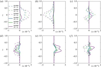
is a cutoff wavenumber. We plot these terms in figure 10 for
 $Ri_{b}=0.40$
,
 $E_{0}=2\times 10^{-5}$
and
 $\mathit{Re}=4000$
, 6000 and 8000 at the approximate times when growth rates of
 $E_{2D}$
and
 $E_{3D}$
are largest (i.e.
 $t\sim 7$
for (a–c) and
 $t\sim 25$
for (d–f)). The cutoff wavenumber is chosen to be
 $k_{c}=2$
.
We observe that, consistent with the results of Kaminski et al. (Reference Kaminski, Caulfield and Taylor2014), the initial two-dimensional energy growth is largely due to shear production, with buoyancy flux acting to convert kinetic energy into potential energy. At later times when the three-dimensional motions are growing, shear production is acting to decrease energy, while buoyancy flux is leading to conversion of potential energy into kinetic energy, consistent with the development of convectively unstable regions of the flow (see figure 3). In addition, there is a net transfer of energy from larger to smaller scales via the nonlinear transfer term. The down-scale energy transfer is seen at earlier times for the case with
 $\mathit{Re}=8000$
. Altogether, the spectral energetics suggest that the secondary instabilities and subsequent three-dimensionalization arise as a result of the nonlinear development of the linear optimal perturbation itself, rather than due to linear instability arising on the nonlinearly modified base flow shown in figures 6 and 7. In fact, at the time when the mean
 $Ri_{g}$
first drops below
 $1/4$
, the shear production term is negative for both the low- and high-wavenumber components of the flow.
High- and low-wavenumber contributions to perturbation energy growth when growth of
 $E_{2D}$
(a–c) and
 $E_{3D}$
(d–f) are maximum, for
 $Ri_{b}=0.40$
,
 $E_{0}=2\times 10^{-5}$
and
 $\mathit{Re}=4000$
, 6000 and 8000. (a,d) Shear production terms,
 ${\mathcal{P}}_{low}$
and
 ${\mathcal{P}}_{high}$
. (b,e) Buoyancy flux terms,
 ${\mathcal{B}}_{low}$
and
 ${\mathcal{B}}_{high}$
. (c,f) Nonlinear transfer terms
 ${\mathcal{T}}_{low}$
and
 ${\mathcal{T}}_{high}$
. For the cases plotted here, the cutoff wavenumber is chosen to be
 $k_{c}=2$
.

Mixing efficiency is an important metric characterizing the proportion of energy expended by a fluid in mixing the density field to the total energy lost to mixing and dissipation (Peltier & Caulfield Reference Peltier and Caulfield2003). One way to consider this is by comparing the dissipation of potential energy to the total dissipation (see e.g. Brucker & Sarkar Reference Brucker and Sarkar2007). Defining the time- and domain-integrated (perturbation) dissipations
 ${\mathcal{E}}_{k}=\int _{0}^{t_{f}}\int _{0}^{L_{z}}\unicode[STIX]{x1D700}_{k}\,\text{d}z\,\text{d}t$
and
 ${\mathcal{E}}_{p}=\int _{0}^{t_{f}}\int _{0}^{L_{z}}\unicode[STIX]{x1D700}_{p}\,\text{d}z\,\text{d}t$
, where
 $t_{f}$
is the end time of the simulation, we can quantify the relative importance of potential energy dissipation to total dissipation via a ‘mixing efficiency’, which we define as
 $$\begin{eqnarray}\unicode[STIX]{x1D702}_{\unicode[STIX]{x1D700}}=\frac{{\mathcal{E}}_{p}}{{\mathcal{E}}_{k}+{\mathcal{E}}_{p}}.\end{eqnarray}$$
In the above,
 $t_{f}$
denotes the end time of the simulation, where the end of the simulation occurs when the fluctuation energy as well as the kinetic and potential energy dissipation terms are small, and the transient turbulence has relaminarized, as is characteristic of such free shear flows. In all cases,
 $\text{d}{\mathcal{E}}_{k}/\text{d}t<0.005{\mathcal{E}}_{k}$
and
 $\text{d}{\mathcal{E}}_{p}/\text{d}t<0.005{\mathcal{E}}_{p}$
by time
 $t_{f}$
.
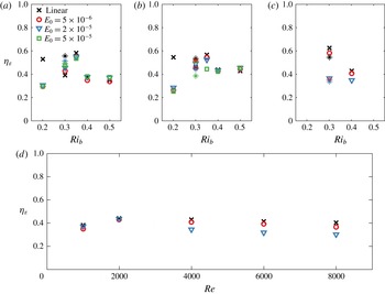
Figure 11 shows this mixing efficiency calculated for a range of
 $\mathit{Re}$
,
 $Ri_{b}$
, and initial amplitude
 $E_{0}$
. It also shows the mixing efficiency as calculated for a purely linear flow evolution; it should be noted that as the linear quantities are ratios of very small numbers associated with quantities, the ratio itself may be relatively high despite the magnitudes of the perturbation dissipation rates being quite low. The linear mixing efficiencies in figure 11 show that, for
 $Ri_{b}\leqslant 0.35$
,
 $\unicode[STIX]{x1D702}_{\unicode[STIX]{x1D700}}\sim 0.5{-}0.6$
, and
 $\unicode[STIX]{x1D702}_{\unicode[STIX]{x1D700}}\sim 0.4$
for
 $Ri_{b}>0.35$
; these values are not strongly dependent on
 $\mathit{Re}$
. In general, across the range of
 $Ri_{b}$
considered here, it is expected that the kinetic and potential energy dissipations will be of similar magnitudes in the case of purely linear flow evolution.
For the direct numerical simulations, the mixing efficiency deviates from the linear values as nonlinear effects become increasingly important. For the lower-
 $\mathit{Re}$
cases (figure 11
a,b), the curves collapse to the linear value for
 $Ri_{b}\geqslant 0.40$
. For
 $Ri_{b}<0.40$
, the mixing efficiency approaches the linear value as
 $Ri_{b}$
increases and
 $E_{0}$
decreases; conversely, for high
 $E_{0}$
and low
 $Ri_{b}$
, nonlinear effects become much more important and mixing efficiency becomes substantially lower than the linear value. The exception to this trend is for
 $Ri_{b}=0.30$
in the smaller domain (
 $L_{x}=9.44$
) at
 $\mathit{Re}=1000$
and 2000, for which the mixing efficiency increases slightly with
 $E_{0}$
due to an increase in
 ${\mathcal{E}}_{p}$
relative to
 ${\mathcal{E}}_{k}$
. We find that
 ${\mathcal{E}}_{p}$
reaches a maximum (
 $\text{d}{\mathcal{E}}_{p}/\text{d}t\approx 0$
) around the time at which the turbulent kinetic energy reaches its maximum value. While there is no evidence of transition to turbulence for these Reynolds numbers, as
 $E_{0}$
is increased the perturbation evolution does lead to some local modification of the background flow, strengthening buoyancy gradients and consequently leading to the observed increase in
 ${\mathcal{E}}_{p}$
. For
 $Ri_{b}=0.20$
, where the initial condition gives rise to the Kelvin–Helmholtz instability and becomes nonlinear for all initial perturbation amplitudes considered here, the resulting mixing efficiency is also significantly lower (
 $\unicode[STIX]{x1D702}_{\unicode[STIX]{x1D700}}\sim 0.30$
) than the value predicted by the purely linear flow evolution. Similar results are seen at
 $\mathit{Re}=4000$
, with a decrease in mixing efficiency seen even for
 $Ri_{b}=0.40$
and
 $E_{0}=2\times 10^{-5}$
, where nonlinear effects are significant, as shown in figures 3, 6 and 7 – the mixing efficiency in this case drops to approximately
 $\unicode[STIX]{x1D702}_{\unicode[STIX]{x1D700}}\sim 0.35$
, as does the mixing efficiency calculated for
 $Ri_{b}=0.30$
and
 $\mathit{Re}=4000$
for both domain sizes
 $L_{x}$
. At higher values of
 $\mathit{Re}$
, the mixing efficiency tends towards a value of approximately 0.30, and the nonlinear values begin to deviate more from the linear values at lower initial amplitudes (figure11
d). While lower than the mixing efficiency in the linear cases, these values of the mixing efficiency are still quite large when compared to the commonly used value of
 $1/6$
, but consistent with Mashayek et al. (Reference Mashayek, Caulfield and Peltier2013) and the more recent results of Maffioli, Brethouwer & Lindborg (Reference Maffioli, Brethouwer and Lindborg2016) and Venayagamoorthy & Koseff (Reference Venayagamoorthy and Koseff2016).
For all of the flows considered, the region of elevated kinetic energy dissipation is localized in the vertical around the centre of the shear layer, as seen in figure 8. The decrease in mixing efficiency seen in figure 11 is associated with flows that experience significant nonlinearity and therefore an elevated kinetic energy dissipation relative to potential energy dissipation as seen in figure 9. In these flows, figure 6 shows that the centre of the shear layer becomes less stratified than the surrounding fluid as the perturbations evolve. While more kinetic energy is being dissipated by the strongly nonlinear flows, comparing figures 6 and 8 shows that the bulk of the dissipation is occurring in a weakly stratified region of fluid, and so the resulting mixing is less efficient than if it were occurring in a more strongly stratified flow.
Mixing efficiency
 $\unicode[STIX]{x1D702}_{\unicode[STIX]{x1D700}}$
, as defined in (3.18), as a function of
 $Ri_{b}$
for different initial amplitudes
 $E_{0}$
and (a)
 $\mathit{Re}=1000$
, (b)
 $\mathit{Re}=2000$
and (c)
 $\mathit{Re}=4000$
. Open symbols correspond to simulations with
 $L_{x}=9.44$
; asterisks denote mixing efficiencies from simulations with
 $L_{x}=12.6$
and
 $Ri_{b}=0.30$
. (d) Mixing efficiency for
 $Ri_{b}=0.40$
as a function of
 $\mathit{Re}$
.

4 Discussion and conclusions
We have computed the linear optimal perturbations – that is, the perturbations that experience the largest linear energy growth – of a stably stratified shear flow for a target time
 $T=15$
advective time units. The linear optimal perturbations have been computed for various bulk Richardson numbers ranging from
 $Ri_{b}=0.20$
to
 $Ri_{b}=0.50$
and for Reynolds numbers from
 $\mathit{Re}=1000$
up to
 $\mathit{Re}=8000$
in some cases. We then used these optimal perturbations as an initial condition for direct numerical simulation with varying initial amplitude in order to examine what, if any, nonlinear effects may occur during the evolution of the flow.
We find that substantial perturbation energy gains are possible, and the maximum linear gain at the target time increases with increasing
 $\mathit{Re}$
and decreasing
 $Ri_{b}$
. Additionally, the structure of the optimal perturbations is sensitive to
 $\mathit{Re}$
,
 $Ri_{b}$
and domain size. However, in all cases considered here
 $O(10^{1}{-}10^{2})$
energy gain is achieved in the purely linear case.
The effects of varying
 $\mathit{Re}$
,
 $Ri_{b}$
, and initial amplitude
 $E_{0}$
are also apparent when the perturbations are allowed to evolve nonlinearly. In general, cases with higher
 $E_{0}$
and
 $\mathit{Re}$
and lower
 $Ri_{b}$
are prone to stronger nonlinear effects, including modification of the mean flow, formation of billows, vigorous secondary instabilities, three-dimensionalization of the flow and break down into smaller-scale structures, leading to enhanced yet transient turbulent dissipation. In some cases, the perturbation evolution may undergo a regime shift with increasing nonlinearity, from a case in which the perturbations generate strong internal waves propagating away from the shear layer to one in which dissipation dominates the energetics. In addition, flows which are susceptible to strongly nonlinear effects exhibit less efficient mixing as a result of higher viscous dissipation.
Here, we have focused primarily on the evolution of quasi-two-dimensional linear optimal perturbations for a target time of
 $T=15$
, which attain close to maximum transient growth for the hyperbolic-tangent stratified shear layer (Kaminski et al.
Reference Kaminski, Caulfield and Taylor2014). As we show in appendix B, despite lower perturbation energy gains the inherently three-dimensional perturbations corresponding to a target time of
 $T=5$
may also lead to saturation and modification of the mean flow. Additionally, substantial transient growth may occur over a range of different perturbation wavelengths (see, for instance, the computed gains for different-sized domains in appendix A, or the results for unstratified flows in Arratia et al. (Reference Arratia, Caulfield and Chomaz2013)) – the nonlinear evolution described above is not restricted only to a certain wavelength or target time. Altogether, it appears that non-normal perturbation growth may lead to significant nonlinear effects for a variety of different initial conditions, even in flows stable to normal-mode perturbations. Further nonlinear simulations of optimal perturbations with a variety of initial wavelengths and target times would therefore be of great interest, in particular to examine any correlation between the length scales of the initial perturbations with those observed during the transition process.
It is natural to question what would happen for flows with even higher
 $\mathit{Re}$
and
 $\mathit{Pr}$
than those considered here, which would be more relevant for the geophysical flows motivating this study. As figure 1(b) shows, the maximum perturbation gain increases with increasing
 $\mathit{Re}$
, and as we have discussed above the onset of secondary instabilities and mixing of the mean flow are also strongly affected by increasing
 $\mathit{Re}$
(as shown, for example, in figure 11).
To examine further what might happen at higher
 $\mathit{Re}$
, we can consider a case in which
 $\mathit{Re}=6000$
,
 $Ri_{b}=0.40$
and
 $E_{0}=2\times 10^{-6}$
(a smaller initial amplitude than the cases considered above). For this set of parameters, by
 $t=6.0$
the gradient Richardson number of the flow is everywhere greater than
 $1/4$
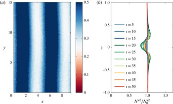
, as seen in figure 12. Unlike the case considered in figure 3 or the higher-
 $\mathit{Re}$
cases described in figures 5 and 10, this flow does not fully develop into billows or break down into turbulence. However, the perturbation does grow enough to modify the mean flow as seen in figure 12(b). In fact, more modification of the base flow occurs in this case than in the flow shown in figure 6(b), despite the initial perturbation amplitude being a factor of 10 lower in figure 12. This points to transient non-normal perturbation growth as a possible mechanism to trigger turbulence and mixing in stably stratified geophysical environments.
It should be noted that a similar dependence on Reynolds number has been observed when considering transition to turbulence in unstratified flows. For example, Reddy et al. (Reference Reddy, Schmid, Baggett and Henningson1998) shows a decrease in the required amplitude for transition with increasing
 $\mathit{Re}$
due to linear optimal perturbations in Poiseuille and Couette flow. Similarly, Duguet et al. (Reference Duguet, Monokrousos, Brandt and Henningson2013) and Cherubini et al. (Reference Cherubini, De Palma and Robinet2015) find that the required perturbation amplitude for transition to turbulence triggered by nonlinear optimal perturbations in plane Couette and boundary layer flows, respectively, decreases with increasing
 $\mathit{Re}$
. Furthermore, Chapman (Reference Chapman2002) derives asymptotically the scaling of the decrease in initial perturbation amplitude with various negative powers of
 $\mathit{Re}$
for subcritical transition to sustained turbulence in plane Couette and plane Poiseuille flow. As such, our observation that nonlinear effects can be observed at lower initial amplitudes for higher-
 $\mathit{Re}$
stratified flows is consistent with these past results.
Gradient Richardson number and buoyancy frequency for
 $\mathit{Re}=6000$
,
 $Ri_{b}=0.40$
and
 $E_{0}=2\times 10^{-6}$
. (a) Local gradient Richardson number on a horizontal plane passing through
 $z=0$
at
 $t=6.0$
. Note that the white region corresponds to
 $Ri_{g}=1/4$
. (b) Evolution of scaled mean buoyancy frequency,
 $N^{\ast 2}/N_{0}^{\ast 2}=\unicode[STIX]{x2202}b/\unicode[STIX]{x2202}z$
, in region around shear layer.

In all of our simulations, the Prandtl number has been held fixed at a value of
 $\mathit{Pr}=1$
, and examining the role of
 $\mathit{Pr}$
in both the linear and nonlinear behaviour of the optimal perturbations would be of great interest. In particular, recent work examining Kelvin–Helmholtz-unstable flows (Salehipour, Peltier & Mashayek Reference Salehipour, Peltier and Mashayek2015) suggests that the preferred secondary instabilities (and therefore the process by which free stratified shear flows undergo the transition to transient turbulence) as well as the mixing efficiency may depend strongly on
 $\mathit{Pr}$
. Examining the nonlinear evolution of linear optimal perturbations at different values of
 $\mathit{Pr}$
for the more strongly stratified flows considered here may also reveal a similar dependence on Prandtl number.
An additional point of interest is the emergence of billows as the result of transient perturbation energy growth in flows with
 $Ri_{b}>1/4$
. It is interesting to compare the billows seen in figure 3 to those arising from the canonical Kelvin–Helmholtz instability. While the billows seen at
 $Ri_{b}=0.40$
have a higher aspect ratio than those arising in a more weakly stratified environment, the resemblance is still remarkable, despite a different physical mechanism leading to their formation.
Despite the fact that the predicted growth rate of the normal-mode Kelvin–Helmholtz instability
 $\unicode[STIX]{x1D70E}_{KH}\rightarrow 0$
as the critical minimum gradient Richardson number of
 $1/4$
is approached, oceanic observations of the turbulence associated with apparently marginal instability (Smyth & Moum Reference Smyth and Moum2013) indicate that the nonlinear billow state has finite amplitude for flows with
 $Ri_{g}$
just below the critical value of
 $1/4$
. This is suggestive of an
 $Ri$
-subcritical transition (as described in the Introduction, with some appropriate Richardson number as the control parameter) where the nonlinear (unstable) billow state commonly referred to as the ‘KH billow’ exists above an as yet unknown threshold
 $Ri^{-1}>Ri_{KH}^{-1}$
. For
 $Ri^{-1}>4$
, the flow is linearly unstable and approaches the billow state transiently, attaining some maximum amplitude, before secondary instabilities onset. However, for
 $Ri_{KH}^{-1}<Ri^{-1}<4$
, only sufficiently large amplitude perturbations approach the billow state, (once again attaining transiently some maximum, non-trivial amplitude) while smaller perturbations are attracted back to the linearly stable laminar state.
It is important to reiterate that the billow state itself is an unstable state embedded within an inherently transient flow, in that it is typically prone to a ‘zoo’ of secondary instabilities and the (unforced) flow will inevitably decay back to the laminar state. Therefore, it is not appropriate to assert that this ‘
 $Ri$
-subcritical’ transition corresponds formally to a canonical subcritical bifurcation of a dynamical system. Nevertheless, the billow state is an identifiable intermediate state of the transient flow evolution for at least some range of Richardson numbers, and our results support the above-described scenario that the nonlinear billow state persists for Richardson numbers greater than those associated with linear instabilities of the laminar state.
Specifically, we observe that the finite-amplitude billow state may be reached for infinitesimal perturbations via the normal-mode instability when
 $Ri^{-1}>4$
. For finite perturbations above a certain initial amplitude, non-normal growth allows perturbations to develop and approach the billow state when
 $Ri_{KH}^{-1}<Ri^{-1}<4$
. We conjecture that the billow state ceases to exist for
 $Ri^{-1}<Ri_{KH}^{-1}$
, in the sense that a flow with such a high Richardson number never approaches a billow-like state at finite amplitude, irrespective of the initial form (or amplitude) of perturbation.
Further examination of the finite-amplitude saturation of perturbations for base flows with
 $Ri_{g,min}\sim 1/4$
would help to clarify the details of the (maximum in time) amplitude of the billow state, and in particular to identify the value
 $Ri_{KH}^{-1}<4$
(which may be a function of
 $\mathit{Re}$
and/or
 $\mathit{Pr}$
) above which this intermediate billow state is approached. It is important to note again that here we are not referring to a transition to a sustained turbulent state, but rather to the unstable finite-amplitude billow state which is then susceptible to secondary instabilities, leading to a transient period of flow evolution with enhanced dissipation rates compared to the laminar state. However, it is still undoubtedly remarkable that despite the lack of linear instability connection to such a state when
 $Ri^{-1}<4$
, perturbations with a sufficiently large initial amplitude are still able to approach closely to a billow state and become at least ‘Kelvin–Helmholtz-like’ at some point in their transient flow evolution.
It should also be emphasized that larger linear growth does not necessarily imply a more efficient transition to turbulence. For example, in the case of unstratified nonlinear optimal perturbations there may exist quasi-linear optimal perturbations with larger peak energy gains but less efficient transition (Rabin et al.
Reference Rabin, Caulfield and Kerswell2012). Pralits, Bottaro & Cherubini (Reference Pralits, Bottaro and Cherubini2015) have shown that weakly nonlinear optimal perturbations may be able to exploit nonlinear modification of the mean flow to allow for enhanced growth and transition to turbulence at amplitudes for which linear optimal perturbations are unable to lead to transition. Even for the linear optimal perturbations considered here there may be other structures with suboptimal linear gains that are nonetheless able to transition to turbulence from lower initial amplitudes. As such, the amplitudes for which the optimal perturbations are able to transition to turbulence should be viewed, in some sense, as an upper bound for the minimum amplitude for transition to turbulence in these strongly stratified flows: there may exist more efficient mechanisms by which lower-amplitude perturbations may be able to transition. In the language of Pringle & Kerswell (Reference Pringle and Kerswell2010), we do not expect these linear optimal perturbations to be ‘minimal seeds’ for the transition to turbulence, which must be identified using an inherently nonlinear DAL method (Eaves & Caulfield Reference Eaves and Caulfield2015). While we would expect, based on our results above, that transition will occur at lower initial amplitudes for increasing
 $\mathit{Re}$
and decreasing
 $Ri_{b}$
, the exact minimal energy needed for transition remains the topic of future work.
Here, we have considered the stability of stratified shear flows inspired by those observed in geophysical settings. However, further modifications can be made to mimic oceanic and atmospheric flows better. Given the strong
 $\mathit{Re}$
- and
 $Ri_{b}$
-dependence observed above, extending this work to more geophysically relevant parameter regimes is needed before reaching firm conclusions about the importance of the transient growth mechanism in these flows. Additionally, while the base flow considered above is steady and parallel, geophysical flows generally vary in both time and space. Extending this work to more complicated base flows would also be of great interest in applying these results to observations.
Acknowledgements
This manuscript benefited from the constructive comments of the referees. A.K.K. was supported by a NSERC doctoral scholarship. The research activity of C.P.C. and J.R.T. was supported by EPSRC Programme Grant EP/K034529/1, entitled ‘Mathematical Underpinning of Stratified Turbulence’. Input files and code for the simulations presented in this paper can be found at https://doi.org/10.17863/CAM.10373.
Appendix A. Linear perturbation energy gains with different domain sizes
In the above discussion, we have focused primarily on optimal perturbations computed over a domain with
 $L_{x}=9.44$
and
 $L_{y}=15.0$
. However, it has been shown in unstratified flows that the optimal gain can depend strongly on the spatial wavelengths of the initial perturbation (see e.g. Andersson, Berggren & Henningson Reference Andersson, Berggren and Henningson1999; Luchini Reference Luchini2000; Arratia et al.
Reference Arratia, Caulfield and Chomaz2013), and so we consider the optimal gains for different domain sizes here. In figure 13, we show the resulting perturbation energy gains at
 $T=15$
for three different values of the horizontal extent
 $L_{x}$
and two different values of the spanwise extent
 $L_{y}$
for
 $\mathit{Re}=1000$
and
 $\mathit{Re}=2000$
. There is little effect on the maximum linear gain when the spanwise extent is doubled, consistent with the two-dimensional optimal perturbation structure mentioned above.
While varying the horizontal domain size is observed to have an effect on the maximum attainable linear growth, generally speaking
 $G(T)$
remains the same order of magnitude across the sizes considered here. Thus, we would expect growing structures over a variety of wavelengths, rather than restricted to a specific range of length scales.
Perturbation energy gain for a target time of
 $T=15$
and a variety of horizontal and spanwise domain sizes
 $L_{x}$
and
 $L_{y}$
. (a)
 $\mathit{Re}=1000$
. (b)
 $\mathit{Re}=2000$
.

Appendix B. Nonlinear evolution for linear optimal perturbations with target time
$T=5$

In the above discussion, we have considered optimal perturbations corresponding to a target time of 15 advective units, which are primarily two-dimensional in structure. A set of additional simulations, the details of which are presented in table 2, were run for linear optimal perturbations with a target time
 $T=5$
,
 $Ri_{b}=0.30$
and 0.40, and
 $\mathit{Re}=1000$
, 2000 and 4000. The domain size was chosen to be
 $(L_{x},L_{y},L_{z})=(9.44,15.0,30.0)$
, and the grid sizes were selected such that
 $\unicode[STIX]{x0394}x_{min}\leqslant 3\unicode[STIX]{x1D702}$
. Only one initial amplitude (
 $E_{0}=2\times 10^{-5}$
) is considered here. As described in Kaminski et al. (Reference Kaminski, Caulfield and Taylor2014), the perturbations for this target time take the form of rolls tilted against the background shear flow, as with
 $T=15$
, but with significant three-dimensional structure. The computed linear perturbation energy gains are approximately 10–20, as shown in figure 14(a), and increase with increasing Reynolds number.
Parameters for nonlinear simulations of
 $T=5$
optimal perturbations with
 $E_{0}=2\times 10^{-5}$
.
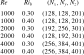
As in figure 4, the nonlinear energy evolution is shown in figure 14(b–d), along with the theoretical linear evolution. As
 $\mathit{Re}$
is increased, the nonlinear fluctuation energy saturates and deviates from the linear predictions, reaching lower peak amplitudes than the linear case but remaining elevated at later times in the flow evolution. The deviation between the linear and nonlinear cases is more pronounced for
 $Ri_{b}=0.30$
than for
 $Ri_{b}=0.40$
. The corresponding kinetic energy dissipation (not shown) reaches peak values comparable to those in figure 8, though the burst of elevated
 $\unicode[STIX]{x1D700}_{k}$
is short lived.
(a) Perturbation energy gain for
 $T=5$
as a function of
 $\mathit{Re}$
. (b–d) Linear and nonlinear perturbation energy evolution for
 $E_{0}=2\times 10^{-5}$
,
 $Ri_{b}=0.30$
and 0.40 and (b)
 $\mathit{Re}=1000$
, (c)
 $\mathit{Re}=2000$
and (d)
 $\mathit{Re}=4000$
. (e,f) Computed linear and nonlinear mixing efficiencies,
 $\unicode[STIX]{x1D702}_{\unicode[STIX]{x1D700}}$
, as a function of
 $\mathit{Re}$
for (e)
 $Ri_{b}=0.30$
and (f)
 $Ri_{b}=0.40$
.

Figure 15 shows the mean scaled buoyancy frequency
 $N^{\ast 2}/N_{0}^{\ast 2}$
and mean gradient Richardson number for the simulations with
 $\mathit{Re}=4000$
. As in figure 6, the perturbation evolution leads to modification of the background buoyancy profile. However, the resulting structure of the mean flow shows two minima located above and below the centre of the shear layer rather the layered profiles seen for the
 $T=15$
cases. The changes in background stratification are less dramatic than those seen in figure 6, and the corresponding mean
 $Ri_{g}$
does not drop below
 $1/4$
.
(a,b) Time evolution of mean scaled buoyancy frequency,
 $N^{\ast 2}/N_{0}^{\ast 2}=\unicode[STIX]{x2202}\overline{b}/\unicode[STIX]{x2202}z$
, for initial perturbations corresponding to a target time
 $T=5$
with
 $E_{0}=2\times 10^{-5}$
,
 $\mathit{Re}=4000$
and (a)
 $Ri_{b}=0.30$
and (b)
 $Ri_{b}=0.40$
. (c,d) Time evolution of mean gradient Richardson number for the same cases i.e. (c)
 $Ri_{b}=0.30$
and (d)
 $Ri_{b}=0.40$
.

The mixing efficiency
 $\unicode[STIX]{x1D702}_{\unicode[STIX]{x1D700}}$
associated with the evolution of the optimal perturbations with
 $T=5$
is shown in figure 14(e,f). Both the linear and nonlinear mixing efficiencies are much lower for the
 $T=5$
linear optimal perturbations (with values of
 $\unicode[STIX]{x1D702}_{\unicode[STIX]{x1D700}}\sim 0.2$
) than for their
 $T=15$
counterparts. This decrease in mixing efficiency is due primarily to higher kinetic energy dissipation relative to potential energy dissipation for the three-dimensional
 $T=5$
perturbations when compared with their two-dimensional
 $T=15$
counterparts. The nonlinear simulations generally have slightly higher mixing efficiencies that the linear predictions, owing to an increase in
 $\unicode[STIX]{x1D700}_{p}$
around
 $t=10$
, when the strongest changes in mean
 $\unicode[STIX]{x2202}B/\unicode[STIX]{x2202}z$
are also occurring (figure 15). It would be interesting to see if, at higher initial amplitude or higher Reynolds number, the nonlinear mixing efficiencies of the
 $T=5$
optimal perturbations further increased to the
 $\unicode[STIX]{x1D702}_{\unicode[STIX]{x1D700}}\sim 0.3$
values seen for
 $T=15$
above and by Maffioli et al. (Reference Maffioli, Brethouwer and Lindborg2016) and Venayagamoorthy & Koseff (Reference Venayagamoorthy and Koseff2016).
It is clear from figures 14 and 15 that the inherently three-dimensional linear optimal perturbations corresponding to shorter target times may also show strongly nonlinear effects at higher
 $\mathit{Re}$
, even for strongly stratified base flows. This may point to transient growth as an important process in normal-mode stable flows over a variety of target times and initial conditions.