


1. Introduction
Knowledge about the characteristics of gas–surface interaction is very important in different fields such as: (i) gas flow at small scales in micro electro-mechanical systems, where the ratio of surface area to corresponding volume is very large compared with conventional devices, (ii) shuttle re-entry and satellite flight, and vacuum technology applications, where the number of molecules in a characteristic volume is relatively low compared with the case of atmospheric working pressure. In all of these applications, the number of the molecule–surface collisions is greater than that of molecule–molecule collisions. In addition, in these kinds of flows, the Knudsen number (Kn), i.e. the ratio of the molecular mean free path to a system's characteristic dimension, is usually larger than one. Therefore, to simulate the gas flow in such conditions, the Boltzmann equation (or other kinetic models) has to be implemented. This equation provides the complete description of the gas flow at the mesoscopic level, but the boundary conditions have to be formulated at the microscopic level. This means that the behaviour of the reflected molecules as a function of the incident molecules has to be known, i.e. a model describing the gas–surface interaction has to be adopted (Cercignani Reference Cercignani1975; Wu & Struchtrup Reference Wu and Struchtrup2017).
The influence of gas–surface interaction has to be accounted for also for when the Knudsen number is lower than one, and this can be done through the velocity and thermal slip coefficients and temperature jump coefficients in the frame of the continuum modelling based on the Navier–Stokes–Fourier system or at higher order, such as the R13 system (Sharipov Reference Sharipov2011; Struchtrup & Taheri Reference Struchtrup and Taheri2011).
In spite of various models describing the interaction between gas molecules and a solid surface, developed during the last fifty years, such as the Epstein model (Epstein Reference Epstein1967), Cercignani–Lampis model (Cercignani & Lampis Reference Cercignani and Lampis1971) and Klinc & Kuščer model (Klinc & Kuščer Reference Klinc and Kuščer1972; Kuščer Reference Kuščer1974), the most largely used is the Maxwell model (Maxwell Reference Maxwell1879). The simplicity of its application as the boundary condition for the Boltzmann equation and other kinetic type equations explains its popularity.
At the microscopic level, when a gas molecule hits a surface, momentum and energy could be transferred during this interaction. Therefore, two accommodation coefficients – accommodation of momentum and of energy – could be introduced to characterize this exchange. However, in the Maxwell model, only one single accommodation coefficient is introduced, without an identification about the nature of the exchange (momentum or energy).
Despite this ambiguous interpretation of the real nature of the exchange (momentum or energy), this Maxwellian model was successfully used to describe various isothermal flows driven by a pressure gradient, both at the microscale and at low pressures (Porodnov et al. Reference Porodnov, Suetin, Borisov and Akinshin1974; Goodman & Wachman Reference Goodman and Wachman1976; Arkilic, Schmidt & Breuer Reference Arkilic, Schmidt and Breuer1997; Colin, Lalonde & Caen Reference Colin, Lalonde and Caen2004; Ewart et al. Reference Ewart, Perrier, Graur and Méolans2006; Graur et al. Reference Graur, Perrier, Ghozlani and Méolans2009). In this case, since the temperature is kept constant in the system, only the momentum exchange is considered to be important and the accommodation coefficient is identified as tangential momentum accommodation coefficient (Agrawal & Prabhu Reference Agrawal and Prabhu2008). In the particular case where only energy exchange takes place between a gas and a surface, without macroscopic gas movement, the thermal or energy accommodation coefficient is introduced in the frame of the Maxwellian model to characterize the particularity of this gas–surface interaction (Teagan & Springer Reference Teagan and Springer1968; Alofs, Flagan & Springer Reference Alofs, Flagan and Springer1971; Saxena & Joshi Reference Saxena and Joshi1981; Trott et al. Reference Trott, neda, Torczynski, Gallis and Rader2011; Yamaguchi et al. Reference Yamaguchi, Imai, Iwai, Kondo, Matsuda and Niimi2014a). However, in the majority of the flows where both exchanges exist, the interpretation of this single coefficient becomes problematic.
The main objective of the present work is in providing a series of data on the mass flow rate of two types of flows: (i) flow driven by a pressure gradient (Poiseuille flow) and (ii) flow driven by a temperature gradient (thermal creep), both of them in the same microchannel, aiming to test different models of the gas–surface interaction. These two types of flows, pressure gradient (Porodnov et al. Reference Porodnov, Suetin, Borisov and Akinshin1974; Arkilic et al. Reference Arkilic, Schmidt and Breuer1997; Colin et al. Reference Colin, Lalonde and Caen2004; Ewart et al. Reference Ewart, Perrier, Graur and Méolans2006; Graur et al. Reference Graur, Perrier, Ghozlani and Méolans2009) and temperature gradient (Porodnov, Kulev & Tuchvetov Reference Porodnov, Kulev and Tuchvetov1978; Rojas Cardenas et al. Reference Rojas Cardenas, Graur, Perrier and Méolans2011; Rojas-Cardenas et al. Reference Rojas-Cardenas, Graur, Perrier and Méolans2013; Yamaguchi et al. Reference Yamaguchi, Imai, Iwai, Kondo, Matsuda and Niimi2014a, Reference Yamaguchi, Perrier, Ho, Méolans, Niimi and Graur2016) driven flows, were studied in the past, but in different channels, thereby the difference in the value of the accommodation coefficients found from these studies could be attributed to the difference in the surface state (surface preparation, roughness, etc.). Therefore, in the present work we offer the experimental results on the mass flow rate for pressure and temperature gradient driven flows in the same microchannel, that is, using an identical surface state.
This paper is organized as follows: first, the experimental set-up is presented and the particularities of both pressure and temperature gradient experiments are discussed. Then, the accommodation coefficients are extracted using the Maxwellian model and data on the mass flow rates obtained from both kinds of experiments. Finally, a first attempt at extraction of two accommodation coefficients (tangential momentum and normal energy) in the frame of the Cercignani–Lampis model is done.
2. Experimental apparatus
The same experimental set-up was used to measure the mass flow rate of the pressure and temperature gradient driven flows. The detailed description of this set-up will be provided in the next section.
2.1. Experimental set-up
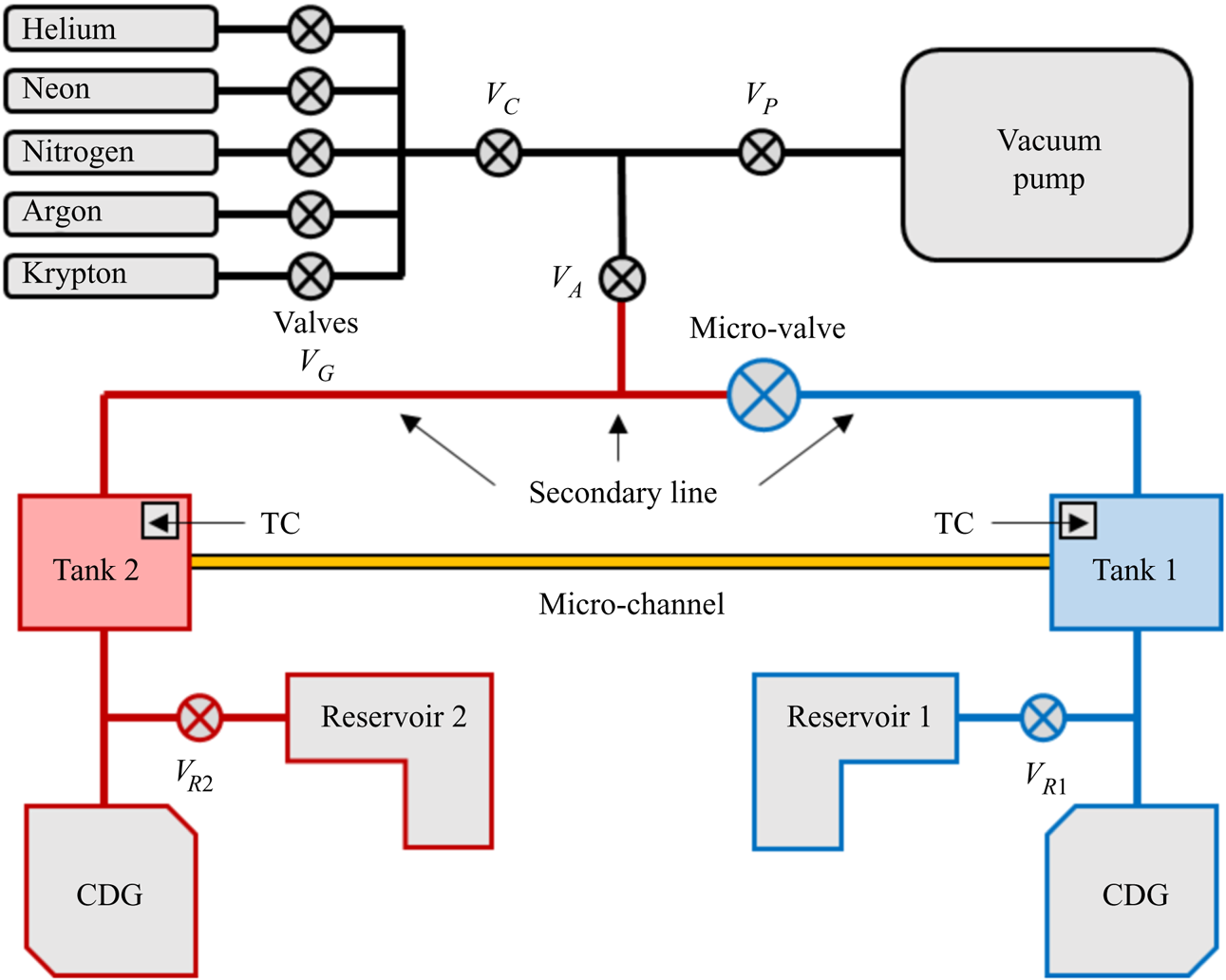
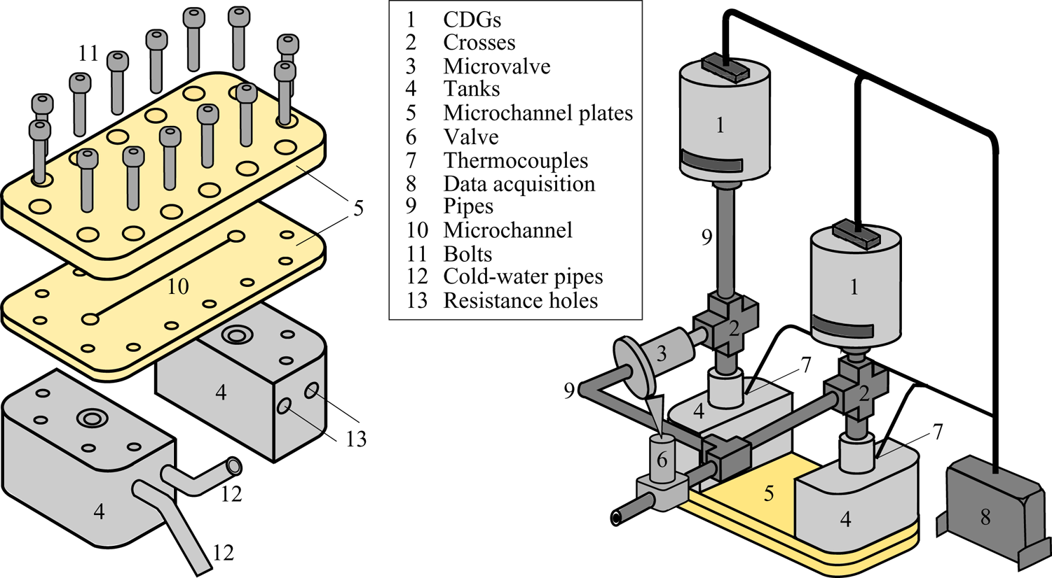
The constant volume methodology (Arkilic et al. Reference Arkilic, Schmidt and Breuer1997; Colin et al. Reference Colin, Lalonde and Caen2004; Ewart et al. Reference Ewart, Perrier, Graur and Méolans2006; Rojas Cárdenas Reference Rojas Cárdenas2012; Yamaguchi et al. Reference Yamaguchi, Perrier, Ho, Méolans, Niimi and Graur2016) is applied to measure the pressure and temperature gradient driven flows through a microchannel. Each one of these two types of experiments was performed separately, i.e. either only a pressure gradient or only a temperature gradient was applied to generate a flow through the microchannel. A scheme representing the experimental set-up is shown in figure 1. It basically consists of two tanks, upstream and downstream tanks, which are connected by the microchannel. The upstream tank, represented in figure 1 by the blue colour (tank 1), is also called the high pressure tank, in the pressure gradient experiments, or the cold tank, in the temperature gradient experiments. The downstream tank, represented by the red colour (tank 2), is also called the low pressure tank in the pressure gradient experiments, or the hot tank, in the temperature gradient experiments. Both upstream and downstream tanks are made of stainless steel and their temperatures can be controlled by circulating water (tank 1, cold side) and by an electrical heater (tank 2, hot side), respectively. The positions of the cooling and heating systems entrances are indicated in figure 2 by the numbers 12 and 13, respectively.
Experimental apparatus used in the pressure and temperature gradient experiments.

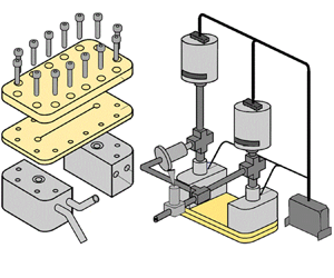
(a) Exploded view of the flat plate, grooved plate and tanks. (b) Tanks and microchannel plates connected to the rest of the system.

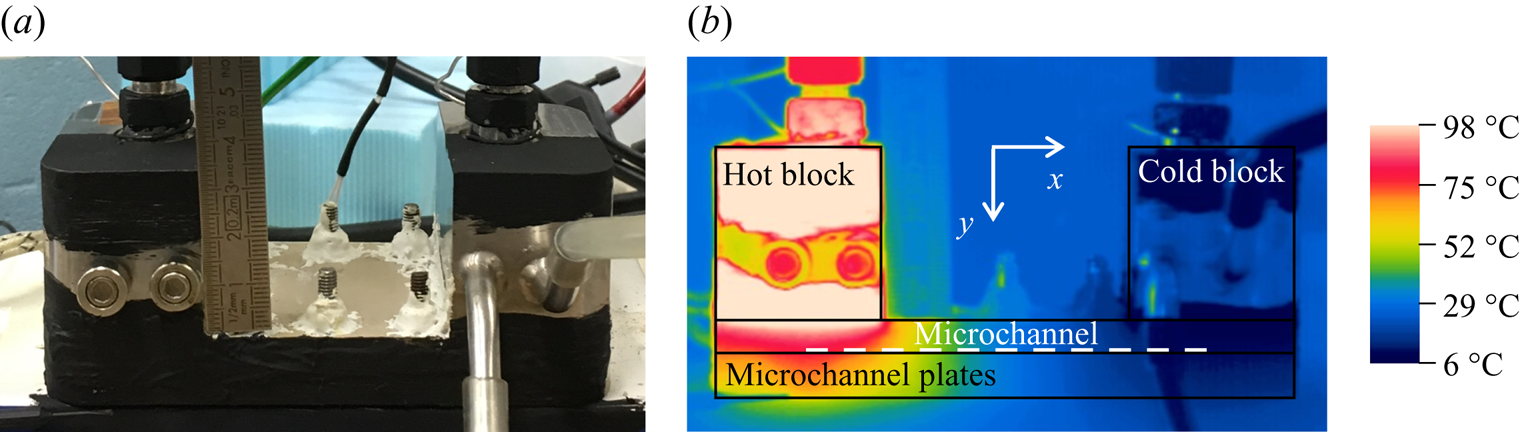
Figure 2(a) presents an exploded view of the microchannel plates and tanks. The microchannel is grooved in the inner plate made in PEEK (polyetheretherketone) and covered by another flat plate of the same material, but thicker than the first one. The interface between the two plates is provided with a flat seal. These two plates are pressed up against each other by fourteen bolts and also pressed against the tanks by eight of these fourteen bolts. To improve the seal and reduce leaks, vacuum glue is added around each external interface and white paste at the top of the threaded rod, see figure 3(a).
(a) Microchannel plates, blocks and part of the pipes and connections coated with a black paint. (b) Temperature field of the system measured by the IR camera for the highest temperature difference,  $\Delta T=67.5\,^{\circ }\textrm {C}$.

The microchannel has a rectangular cross-section with the following dimensions: height  $H=0.24\pm 0.01\ \textrm {mm}$, width
 $W=1.00\pm 0.01\ \textrm {mm}$ and length
 $L=72.00\pm 0.05\ \textrm {mm}$. The roughness of the microchannel, the Ra parameter, was measured with a three-dimensional digital microscope, following the criteria of ISO4287. This standard states that, to obtain a value of roughness from a topography of a sample, first a flatness correction is applied to it and then a set of roughness profiles is extracted. The Ra parameter is the arithmetic average value of the roughness profiles. The roughness was measured in the top and bottom faces of the channel. The roughness parameter for both faces is found to be equal to
 $113\pm 19\ \textrm {nm}$, which is of the order of
 $0.05\,\%$ of the channel height. The roughness of the lateral faces was not measured. Even if the material of the channel walls is the same, the milling process used to manufacture the channel cannot guarantee the same roughness for the horizontal and vertical walls. Since the areas of the lateral faces are much smaller (five times) in comparison with the top and bottom areas, we assume that the absence of this information cannot essentially impact further conclusions about the flow patterns.
Two additional volumes, referenced in the following as reservoirs 1 and 2, figure 1, are connected to tanks 1 and 2, respectively, to increase the total volume of the system. The additional reservoirs are connected to the upstream and downstream tanks by the valves  $V_{R1}$ and
 $V_{R2}$, respectively. Therefore, depending on the position of the valves, these reservoirs can be included or not in the measuring system. For the pressure gradient experiments, the volumes of reservoirs 1 and 2 are equal (
 $208.9\pm 4.5\ \textrm {cm}^3$). For the temperature gradient experiments, we do not use any additional reservoirs in the cold side, while a small reservoir of volume equal to
 $57.6\pm 1.2\ \textrm {cm}^3$ is connected to the hot side. The effect of these additional volumes on the accuracy of mass flow rate measurements and duration of the experiments will be discussed in § 4.2.
The upstream and downstream tanks are connected not only by the microchannel, but also by a large diameter pipe system, called the secondary connection or secondary line, see figure 1. In order to allow or prevent a gas to flow between these two tanks by the secondary connection, a micro-valve was inserted in this circuit. During the pressure gradient experiments, this micro-valve was not used, remaining closed all the time, while in the temperature gradient experiments, this micro-valve was opened in the beginning of each experiment to insure the development of the stationary thermal transpiration flow.
The pressure variation in time in each tank is measured by a high-speed response (30 ms) capacitance diaphragm gauge (CDG), manufactured by Inficon. In the temperature gradient experiments, a single pair of CDGs is used in all the measurements, both of them with a full scale of 1.33 kPa, while in the pressure gradient experiments, three different pairs of CDGs are implemented, with full scales of 133–133 kPa, 133–13.3 kPa and 1.33–1.33 kPa, depending on the desired pressure measurement range.
During the pressure gradient experiments, the cooling and heating systems are switched off and both tanks are kept at the room temperature, while in the temperature gradient experiments both systems work to maintain the tanks at constant but different temperatures. The external temperature of each tank is measured by a K-type thermocouple. Obviously there should be a discrepancy between the measured temperatures (external walls of the tanks) and the temperatures at the microchannel entrances. To associate the measured temperature gradient driven flow with the applied temperature difference at the microchannel ends, the temperature at the microchannel surfaces was measured using an infra-red (IR) camera, and the details of these measurements are provided in § 3. The data measured from the pressure gauges (CDGs) and the thermocouples (TCs) are captured by a data acquisition system produced by the National Instruments Corporation.
The leakage rate in the system was evaluated using 13.3 kPa pressure sensors according to the following procedure: first, all the valves of the experimental set-up, except the valves  $V_{G}$, see figure 1, were opened and the system was pumped down during 72 h using a vacuum pump, model Adixen Drytel 1025. Then, the valves
 $V_{A}$,
 $V_{R1}$ and
 $V_{R2}$ were closed and both CDGs captured the pressure evolution from initial measured pressure of 0.133 Pa for two hours. During this period, the pressure inside the system increased by 0.424 Pa, which is associated with the leakage rate into the system by the gaps of the microchannel plates, figure 2(a), and other connections, see figure 1, and also a possible outgassing. This increase in the pressure corresponds to a mass flow rate of the order of
 $2.18\times 10^{-14}\ \textrm {kg}\ \textrm {s}^{-1}$, which could be associated with a leakage rate into the system and an outgassing. However, the lowest value of mass flow rate measured through the microchannel driven by the temperature gradient was
 $2.88\times 10^{-12}\ \textrm {kg}\ \textrm {s}^{-1}$, which is more than two orders of magnitude larger than the leakage rate. Therefore, the leakages and outgassing were considered as a part of the uncertainties of the pressure driven and temperature driven experiments, see § 4.3.
2.2. Volumes setting for pressure and temperature gradient experiments
The constant volume technique consists of measuring the pressure variation with time between two constant volumes connected by a microchannel (Ewart et al. Reference Ewart, Perrier, Graur and Méolans2007; Rojas Cardenas et al. Reference Rojas Cardenas, Graur, Perrier and Méolans2011; Rojas-Cardenas et al. Reference Rojas-Cardenas, Graur, Perrier and Méolans2013). The total volume  $V_{i}$ connected to the side
 $i$ of the microchannel includes: volume of tank,
 $V_{tank,i}$, volume of additional reservoir,
 $V_{res,i}$, volume of connecting pipes,
 $V_{pipes,i}$, internal volumes of the valves,
 $V_{valves,i}$, and internal volume of pressure transducer,
 $V_{CDG,i}$
 \begin{equation} V_{i}=V_{res,i}+V_{tank,i}+V_{pipes,i}+V_{valves,i}+V_{CDG,i}, \end{equation}
where the subscript  $i$ refers to the upstream (
 $i=1$) and downstream (
 $i=2$) sides of the microchannel, see figure 1. The total volumes of the upstream and downstream sides for all the settings used in the pressure and temperature gradient experiments are provided in table 1. It is clear that the volume of the microchannel,
 $V_{ch}=0.017\ \textrm {cm}^3$, is much smaller compared with the total upstream and downstream volumes.
Total volumes of both upstream and downstream sides,  $V_{1}$ and
 $V_{2}$, respectively, used in the four different settings. The total volume of the system (
 $V_{T}=V_{1}+V_{2}$) and volume ratio (
 $V_{ratio}=V_{1}/V_{2}$) are also presented.

From table 1, it can be realized that the total volumes of the upstream,  $V_{1}$, and downstream,
 $V_{2}$, sides are slightly larger for the two first settings, PG1 and PG2, in comparison with the third one, PG3, even if the same reservoirs are used in all the pressure gradient measurements. This happens because the CDGs with a full scale of 1.33 kPa have internal volumes slightly smaller than the other ones. This table also shows that only one volume setting is implemented in the temperature gradient experiments, since the same pair of CDGs is used in all the measurements.
3. Estimation of temperature profile along the microchannel
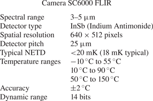
The temperature gradient driven mass flow rate significantly depends on the channel surface temperature, especially on the temperature difference between the channel ends, therefore this temperature has to be measured or, at least, estimated. The measurements of the temperature field in the tanks and of the temperature distribution along the microchannel surface were performed using an IR camera, which characteristics are given in table 2.
Specifications of the IR camera used in the measurements.

The IR camera is calibrated considering a black body. Thus, in order to measure the correct value of temperature, some surfaces of the microchannel plates, tanks, parts of the pipes and connections were coated with a black paint, model Nextel Velvet-Coating 811-21, see figure 3(a). The emissivity of this black paint was measured with an IR spectrophotometer Nexus 670 for a spectral range between  $3$ and
 $5\,\mathrm {\mu }\textrm {m}$, and its value is found to be equal to 0.96.
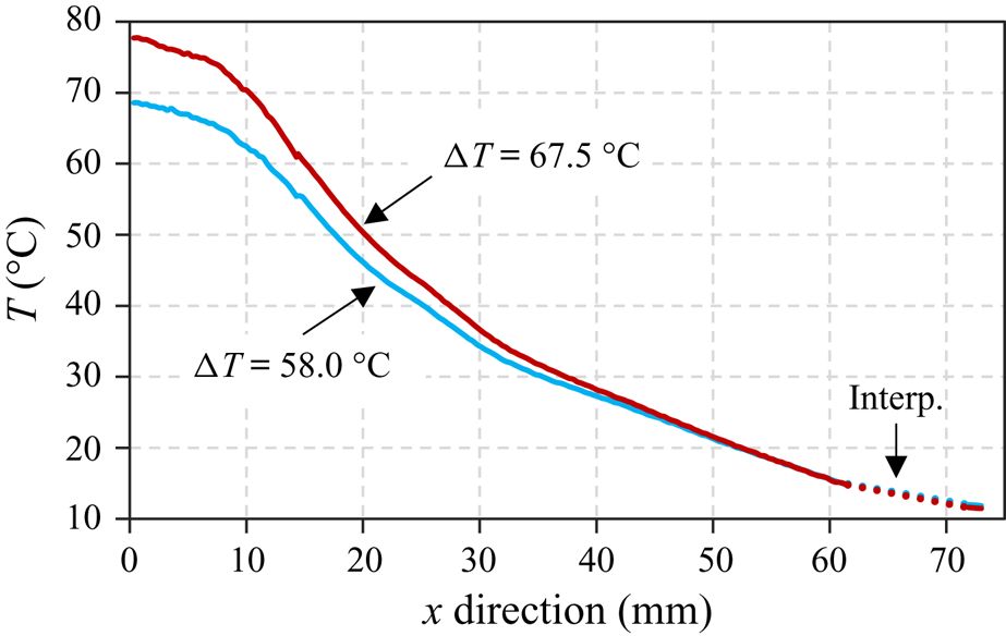
All of the procedure explained in this section refers to the highest temperature difference,  $\Delta T=T_2-T_1=67.5\, ^{\circ }\textrm {C}$, used in the measurements, but the same steps were also performed for the lowest temperature difference as well (
 $\Delta T=58.0\, ^{\circ }\textrm {C}$). Aiming to have an established temperature profile along the microchannel, the electrical resistance and the cold water flux were initialized 18 h before the temperature measurement. During the last two hours of this period, the variation of the temperature measured by the thermocouples at the external walls of the tanks was lower than
 $0.5\,^{\circ }\textrm {C}$. This variation was mostly caused by the change in the room temperature, which is not controlled. The temperature measurements of the same external surfaces of both tanks, were carried out with the IR camera during a short period (around 6 min), which correspond to an average experimental time duration for temperature driven experiments, and the temperature variations on both hot and cold sides did not exceed
 $0.02\,^{\circ }\textrm {C}$. This very small variation confirms the negligible influence of the external convection. The values of temperature measured by the thermocouples and by the IR camera for two applied temperature differences are provided in table 3. The difference between the temperatures obtained by the thermocouples and by the IR camera is lower than
 $3\,^{\circ }\textrm {C}$. This difference is explained because the spots of measurement are not the same, i.e. the thermocouples provide a local measurement of a point on the top part of the tank surface, while the IR camera gives the average temperature of a substantial part of the front surface of each tank. In addition, the measurement uncertainty of the IR camera is 2 K and of the thermocouple is of 0.5 K. The complete explanation of the exact spots of temperature measurements with both thermocouples and IR camera is presented in Brancher (Reference Brancher2019).
Temperatures measured by the IR camera and thermocouples at the external surfaces of both tanks and at the microchannel end (cold and hot sides) cross-section (ECS) for the two temperature differences.

The temperature field of the whole system measured by the IR camera is shown in figure 3(b), where the microchannel is represented by a white dashed line. The temperature at the hot-side cross-section of the microchannel is considerably lower than the external temperature of the hot tank. Although there is also a difference between the external temperature of the cold tank and the temperature at the cold-side cross-section of the microchannel, this difference is much less pronounced compared with that of the hot side.
The values of the average temperatures of microchannel end cross-sections and tanks for both hot and cold sides, for the two temperature differences,  $58.0 \,^{\circ }\textrm {C}$ and
 $67.5 \,^{\circ }\textrm {C}$, are presented in table 3. There is a considerable difference between the surface temperature of the tank measured by the thermocouple at its upper surface and the wall temperature of the microchannel end cross-section measured by the IR camera, mainly for the hot side.
For instance, for the highest temperature difference, the temperature of the top part of the hot tank, measured by the thermocouple, is  $95.5\,^{\circ }\textrm {C}$, while the temperature of the hot-side end cross-section of the microchannel, obtained by the IR camera, is
 $79.0\,^{\circ }\textrm {C}$. These later data of temperature measurements will be used in § 4.2 for the calculations of the mass flow rate for the temperature gradient driven flows.
The temperature profile along the microchannel was also measured by the IR camera at the lateral surface in the interface of the two microchannel plates and it is presented in figure 4. As can be seen in figure 3, the inlet tube of the cooling system of the cold tank disturbs the measurement, since it is located between the IR camera lens and the lateral surface of the microchannel plates. For this reason, the temperature along a segment of approximately 10 mm nearby the cold-side end cross-section of the microchannel was reconstructed by the linear interpolation, dotted line on figure 4.
Temperature gradient along the microchannel for the two temperature differences.

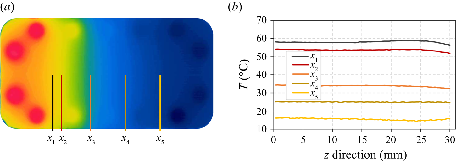
As previously mentioned, the IR camera measures temperature at a surface. Thus, the temperature profile along the microchannel was obtained by measuring the surface temperature at the lateral face of the microchannel plates. Hence, to assume that it is correct to extract the temperature profile along the microchannel from this measurement at the lateral surface, it is necessary to neglect the temperature gradient in the direction perpendicular to this lateral face. The temperature field shown in figure 5 indicates that actually this assumption is correct, since practically there is no difference between the temperature in the centre line of the bottom plate,  $z=0\ \textrm {mm}$, and the temperature in its peripheral region,
 $z=30\ \textrm {mm}$.
Temperature profiles in the  $z$-direction (channel width) of five different microchannel sections for
 $\Delta T=67.5\,^{\circ }\textrm {C}$.

4. Mass flow rate measurements
The mass flow rate through the microchannel can be generated by setting a pressure difference between the tanks (pressure gradient experiments) or a temperature difference (temperature gradient experiments). In both cases, the pressure variation inside the tanks (or the pressure difference between them) is measured, which is due to the mass of gas flowing from the upstream to the downstream tank. In order to relate the pressure variation in time to the mass flow rate, the ideal gas law in each tank is used in the following form:
 \begin{equation} p_i V_i=M_i{\mathcal{R}} T_i, \quad i=1,2, \end{equation}
where  $p_i$,
 $M_i$ and
 $T_i$ are the pressure, mass and temperature of the gas in the tank
 $i$, respectively,
 $V_i$ is the volume of tank
 $i$ and
 ${\mathcal {R}}$ is the specific gas constant. By using the logarithmic derivation of previous equation and assuming the volume constancy we obtain the following expressions:
 \begin{equation} \frac{\textrm{d}p_i}{p_i} = \frac{\textrm{d}M_i}{M_i} + \frac{\textrm{d}T_i}{T_i}, \quad i=1,2. \end{equation}
Finally, rearranging (4.2), we express the mass variation in time in each tank in the form
 \begin{equation} \textrm{d}M_i = \frac{V_i}{{\mathcal{R}} T_i}\, \textrm{d}p_i \left(1-\epsilon_i\right), \quad \epsilon_{i}=\frac{\textrm{d}T_i/T_i}{\textrm{d}p_i/p_i}, \quad i=1,2, \end{equation}
where  $\epsilon _{i}$ is the ratio between the relative temperature and pressure variations in time inside the tank
 $i$. When this ratio is small, i.e. the temperature variation is much smaller than the pressure variation during a specific time interval,
 $\textrm {d}t$, we obtain the expressions of the mass flow leaving tank 1 and entering into tank 2 in following form:
 \begin{equation} {\frac{\textrm{d}M_i}{\textrm{d}t}=\dot M_i = \frac{V_i}{{\mathcal{R}} T_i} \frac{\textrm{d}p_i}{\textrm{d}t}, \quad i=1,2.} \end{equation}
The derived expressions of (4.4) can be used for both pressure and temperature gradient driven flows, under the conditions of small values of  $\epsilon _i$ compared with unity (
 $\epsilon _i\ll 1$). The experimental estimations of the
 $\epsilon _i$ values in the case of the pressure and temperature driven flows are given in § 4.3.
To obtain a pressure variation with time in both reservoirs, an initial pressure difference (pressure gradient experiments) or an initial temperature difference (temperature gradient experiments) must be imposed between the two tanks. Since the behaviour of the pressure inside the upstream and downstream tanks differs from the pressure gradient to the temperature gradient experiments, they will be explained separately.
4.1. Pressure gradient driven flow
A brief explanation of the steps followed during the pressure gradient experiments is given below using the sketch of the experimental set-up presented in figure 1. Firstly, before performing the measurements with a gas, the whole system is pumped down for 12 h with all the valves kept open, except the valves  $V_G$. After this period, the valve
 $V_P$ is closed and one of the valves
 $V_G$ is opened, depending on the gas to be used, to fill the whole system with the chosen gas. Thereafter, the valves
 $V_A$ and
 $V_C$ are closed to stop the connections between the microchannel with the gas bottles and vacuum pump. Additionally, the micro-valve is closed too, then tanks 1 and 2 are connected only through the microchannel. After that, the initial pressure difference
 $\Delta p(t_0)=p_1(t_0)-p_2(t_0)$ (or with other notation:
 $\Delta p_0=p_{1,0}-p_{2,0}$) is imposed between the two tanks by quickly opening and closing the valve
 $V_A$, while the valve
 $V_P$ is kept open. Immediately after the opening and closing of the valve
 $V_A$, at
 $t=t_0$, the pressure inside the downstream tank,
 $p_2$, suffers a drastic reduction, while the pressure inside the upstream tank,
 $p_1$, does not change due to the high restriction imposed by the microchannel. Comments about the possible non-isothermal effects at this stage can be found in Appendix A. After that, for
 $t>t_0$, the pressure inside the upstream tank,
 $p_{1}$, starts to decrease while the pressure inside the downstream tank,
 $p_{2}$, starts to increase, until both pressures reach the same final value,
 $p_{f}$. The time when the pressures in both tanks become equal is denoted
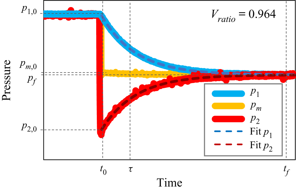
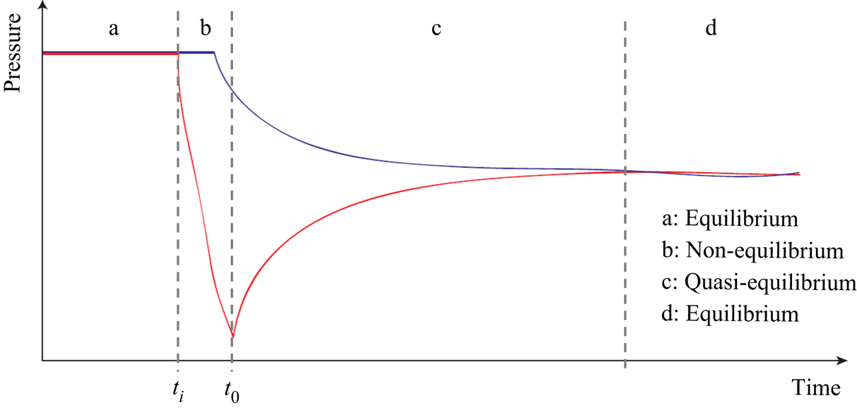
 $t_f$ and its practical definition is given in the end of this section. The behaviour of the pressures inside the two tanks mentioned above for a generic pressure gradient experiment is shown in figure 6. The experiments for other different initial pressures are performed by opening and closing the valve
 $V_A$, keeping the valve
 $V_P$ opened, and waiting to the stabilization of pressures in both tanks.
Behaviour of upstream,  $p_{1}(t)$, downstream,
 $p_{2}(t)$, and mean,
 $p_{m}(t)=0.5(p_1(t)+p_2(t))$, pressures as function of time in a generic pressure gradient experiment. The exponential fittings of
 $p_{1}$ and
 $p_{2}$ are shown by dashed lines.

During the experiments, both tanks are kept at room temperature without any external heat sources. In addition, the amount of gas inside the microchannel is small and cannot change considerably the tank temperature because of the large thermal inertia of the tanks. During each experimental run, the external temperature of each tank was monitored, then its mean value over an experimental duration,  $\bar {T}$, and corresponding standard deviation,
 $s$, are calculated. Both quantities appear as a pertinent evaluation of the probable temperature variations in the tanks as
 $\textrm {d}T_i/T_i\approx s_i/\overline {T_i}$,
 $i=1,2$. These values were found to be less than 0.0002 for both low and high pressure sides and they are associated with the corresponding temperature variations
 $dT_i/T_i$,
 $i=1,2$. The pressure variations in the high pressure tank were found to be in the range of
 $0.03< dp_1/p_1<0.24$, while the pressure variations in the lower tank are higher and were in the range of
 $0.03< dp_2/p_2<0.46$. Therefore, the values of
 $\epsilon _i$ parameters, present in (4.3), are estimated to be in the range of
 $0.0008<\epsilon _1<0.006$ and
 $0.0004<\epsilon _2<0.006$ for the higher and lower pressure tanks, respectively, being very low for all the pressure driven experiments, see table 4. Based on that, the mass flow rate for these experiments can be extracted from the measurements of pressure variation in any of the tanks, using one of (4.4).
Measurement of uncertainties of mass flow rate, when the pressure exponential evolution inside the tanks is used for the calculation. The results are presented for pressure (PGDF) and temperature (TGDF) gradient driven flows.

To obtain the mass flow rate through the microchannel from (4.4), the derivative of the pressure in time must be calculated. According to Rojas-Cárdenas et al. (Reference Rojas-Cárdenas, Silva, Ho, Deschamps and Graur2017) and Johansson et al. (Reference Johansson, Testa, Zaier, Perrier, Bonnet, Moulin and Graur2018), we assume that the pressure variation in the upstream and downstream tanks can be represented as exponential functions in the following form:
 \begin{align} p_1(t) &= p_f +
(p_{1,0}-p_f) \exp (-(t-t_0)/\tau_1),\notag\\ p_2(t) &= p_f +
(p_{2,0}-p_f) \exp (-(t-t_0)/\tau_2),
\end{align}
where  $\tau _1$ and
 $\tau _2$ are the pressure relaxation times for the upstream and downstream tanks, respectively. The exponential form of pressure variation in time, (4.5a,b), was obtained under the assumption of constancy of the pressure relaxation time during an experiment (Johansson et al. Reference Johansson, Testa, Zaier, Perrier, Bonnet, Moulin and Graur2018). The pressure difference between the tanks can be presented analogously as
 \begin{equation} \Delta p(t) = \Delta p(t_0)\exp (-(t-t_0)/\tau). \end{equation}
As this relaxation time depends on the mean pressure, the constancy of the mean pressure in time insures the constancy of  $\tau$, and so the validity of (4.5a,b). In the following, we derive the conditions of the mean pressure constancy in the pressure driven experiments.
From the ideal gas law, (4.1), and considering the mass conservation along the microchannel at any time, it is possible to obtain an expression relating the pressure variation in both tanks,  $\textrm {d}p_{1}$ and
 $\textrm {d}p_{2}$, with the volume ratio
 $V_{ratio}=V_1/V_2$, when the tanks are kept at the same temperature
 \begin{equation} \textrm{d}p_1 V_1={-}\textrm{d}p_2 V_2. \end{equation}
By integrating the previous relation from the initial stage of an experiment, with pressures  $p_{1,0}=p_1(t_0)$ and
 $p_{2,0}=p_2(t_0)$, to the final stage, when the pressures are equal in both tanks,
 $p_1(t_f)=p_2(t_f)=p_f$, we obtain the following expression:
 \begin{equation} \frac{p_{1,0} - p_f}{p_f - p_{2,0}} = \frac{V_2}{V_1}, \end{equation}
which allows us to control the amplitude of the pressure variation in both tanks between its initial value,  $p_{i,0}$, and its final value,
 $p_f$, by changing the volume ratio. From (4.8), it is still possible to obtain another expression to calculate the variation of the mean pressure from the beginning of the experiment,
 $p_{m,0}=0.5(p_{1,0}+p_{2,0})$, to its end,
 $p_{m,f}=p_f$, as
 \begin{equation} \frac{p_f}{p_{m,0}} = \frac{2 ( 1 + V_{ratio} p_{ratio}) }{(1 + V_{ratio})(1 + p_{ratio})}, \end{equation}
where  $p_{ratio}=p_{1,0}/p_{2,0}$. When the volumes are equal, it follows from (4.9) that the mean pressure does not vary during an experiment and
 $p_f=p_{m,0}$. Considering that the total volumes of each side of the microchannel are different, that is
 $V_{ratio}$ is different from 1, the mean pressure may vary during an experiment. From a known volume ratio and using (4.9), we can calculate the maximum initial pressure ratio which ensures the mean pressure constancy with some given accuracy. The volume ratio,
 $V_{ratio}$, used in the pressure gradient experiments, is equal to 0.964, see table 1, thus ensuring a maximal mean pressure variation of the order of
 $1\,\%$, according to (4.9), we have to set the initial pressure ratio,
 $p_{ratio}$, less than 3.45. Therefore, in all the experiments this pressure ratio was fixed smaller than 3.
In practice, we have to define a time interval to fit the pressure (or pressure difference variation) in time for each experimental run. In pressure driven experiments, we fit the values of the pressure difference up to time moment  $t_{\tau }$ defined as
 $\Delta p(t_{\tau })=\varepsilon _{\tau }\Delta p(t_0)$, where
 $\varepsilon _{\tau }$ is a low value parameter. As the pressure difference between the tanks follows an exponential decay, (4.6), we associate this time
 $t_{\tau }$ with the relaxation time as
 $t_{\tau }=t_0-\tau \ln {\varepsilon _{\tau }}$. In experiments, we fix the value of
 $\varepsilon _{\tau }$ equal to 0.02, so the fitting time becomes
 $t_{\tau }=t_0+3.9\tau$. The final experimental time is usually longer than the fitting time and it is defined as
 $t {_{{f}}}=t_0+7\tau$, which corresponds to 0.1 % of the deviation of the pressure difference from zero. This
 $t {_{{f}}}$ parameter is the time where the pressure equilibrium is asymptotically reached. Since the final time is proportional to the relaxation time, it depends on the gas species, pressure level and reservoir sizes.
Respecting the condition for the constancy of the pressure relaxation time and using the mass conservation property we can write that  $\tau _1=\tau _2=\tau$. By calculating the derivative of pressure variation in time, (4.5a,b), and replacing it in (4.4), we obtain the expressions for the mass flow rate in each tank
 \begin{align} \dot M_1(t) = \frac{V_1}{{\mathcal{R}} T} \frac{{p_f-p_{1,0}}}{\tau} \exp \left(-\frac{(t-t_0)}{\tau} \right), \quad \dot M_2(t) = \frac{V_2}{{\mathcal{R}} T} \frac{p_{f}-p_{2,0}}{\tau} \exp \left(-\frac{(t-t_0)}{\tau} \right). \end{align}
As was explained in Johansson et al. (Reference Johansson, Testa, Zaier, Perrier, Bonnet, Moulin and Graur2018), in the case of isothermal flow, the mass flow rate can be also calculated from the pressure difference variation in time,  $\Delta p(t)=p_1(t)-p_2(t)$, as follows:
 \begin{equation} \dot M(t) = \frac{V_0}{{\mathcal{R}} T} \frac{\Delta p_{0}}{\tau} \exp \left(-\frac{(t-t_0)}{\tau} \right), \quad V_0=\frac{V_1 V_2}{V_1+V_2}, \end{equation}
where  $V_0$ is the reduced volume. From the mass conservation property we have
 ${-}\dot M_1(t)=\dot M_2(t)=\dot M(t)$. This equality is satisfied in the steady-state flow regime.
4.2. Temperature gradient driven flow
It is known that when a temperature gradient is applied along the axis of a microchannel connected to two reservoirs of infinite volume maintained at the same pressure but at different temperatures, the gas inside this channel flows continuously from the colder to the hotter side (Reynolds Reference Reynolds1879). This phenomenon is called thermal transpiration. When the volumes connected by a microchannel are finite, a counterflow from the hot to the cold tank is generated, which leads to a steady-state situation, when the temperature gradient driven flow is counterbalanced by the pressure gradient driven flow, and the total mass flow rate through a channel becomes zero.
A short description of the specificity of the temperature gradient driven flow experiments is presented below. Firstly, before performing the measurements with a certain gas, the water cooling of the upstream tank (tank 1 or cold tank) and the electrical heater inserted in the downstream tank (tank 2 or hot tank) are turned on. After that, the whole system is connected to the vacuum pump for 12 h, as was done for the pressure gradient experiments. After that, the temperatures of both tanks are stabilized and the whole system is under vacuum conditions. Then, the system is filled with the gas to be tested, by following the same steps as was done for the pressure gradient experiments. After the chosen working gas fills the system, the valve  $V_A$ is closed, see figure 1. At this moment, even with the imposed temperature difference between the hot and cold tanks, the gas pressure inside both tanks is exactly the same, since the micro-valve is still open, and, consequently, the gas can flow from one tank to another not only through the microchannel but also through the secondary line (a large diameter pipe system), see figure 1. This fact of the pressure equality,
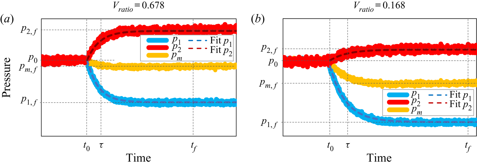
 $p_1(t)=p_2(t)=p_0$, can be clearly seen in figure 7, when
 $t< t_0$.
Behaviour of cold-side,  $p_{1}(t)$, hot-side,
 $p_{2}(t)$, and mean,
 $p_{m}(t)$, pressures as functions of time in a generic temperature gradient experiment for two different volume ratios: (a)
 $V_{ratio}=0.678$ and (b)
 $V_{ratio}=0.168$. The exponential fittings of
 $p_{1}(t)$ and
 $p_{2}(t)$ are also shown by the dashed lines.

At time  $t_0$, the micro-valve is closed. From this moment, the two tanks are connected only by the microchannel, where the gas flows from the cold side to the hot one, so the thermal transpiration flow (Reynolds Reference Reynolds1879; Rojas Cardenas et al. Reference Rojas Cardenas, Graur, Perrier and Méolans2011) takes place in the microchannel. This thermal creep flow immediately generates an increase in the pressure inside the hot tank and a decrease in the pressure inside the cold tank. This pressure difference between the tanks leads to the appearance of a counterflow, so-called Poiseuille flow, from the high pressure side to the low pressure one, that is in the opposite direction to the thermal transpiration flow. To sum up, from time
 $t_0$, there is an increase in pressure
 $p_2(t)$ (hot tank) and a decrease in pressure
 $p_1(t)$ (cold tank), as can be seen in figure 7(a).
When the Poiseuille flow reaches the same magnitude as that of the thermal transpiration flow, the net mass flow rate through the microchannel becomes zero and the pressures inside both tanks achieve constant but different values,  $p_{1,f}$ and
 $p_{2,f}$, in the cold and hot reservoirs, respectively, as can be seen in figure 7(a). As for the pressure driven flow, see § 4.1, we define the final experimental time in terms of the relaxation time as
 $t {_{{f}}}=7\tau +t_0$. Also, in the temperature driven experiments, the fitting of the pressure variation in the cold tank is done during the fitting time
 $t_{\tau }$, which is calculated for this tank as
 $p_1(t_{\tau })-p {_{{f}}}=\varepsilon _{\tau }(p_{1,0}-p {_{{f}}})$, with
 $\varepsilon _{\tau }=0.02$.
When this zero flow condition is achieved, an important characteristic of the temperature gradient driven flow can be obtained, the thermomolecular pressure difference (TPD), which is defined by the difference between the pressures inside the hot and cold tanks, respectively, according to the following expression:
 \begin{equation} \textrm{TPD} = p_{2,f} - p_{1,f} = \Delta p_1 + \Delta p_2, \end{equation}
where  $\Delta p_1=p_0-p_{1,f}$ and
 $\Delta p_2=p_{2,f}-p_0$.
Since the temperatures of each tank are constant during an experiment, we can use the same reasoning as presented in § 4.1 and make use of expressions (4.4) to calculate the mass flow rate if the ratios of the thermal fluctuations to the pressure fluctuations, i.e.  $\epsilon _i$ (
 $i=1,2$), (4.3), are small enough compared with unity. The estimations of
 $\epsilon _i$ are provided in § 4.2.1.
The pressure variation inside both cold and hot tanks can be approximated using the relations (Rojas-Cardenas et al. Reference Rojas-Cardenas, Graur, Perrier and Méolans2012, Reference Rojas-Cardenas, Graur, Perrier and Méolans2013; Yamaguchi et al. Reference Yamaguchi, Rojas-Cardenas, Perrier, Graur and Niimi2014b)
 \begin{align} p_1(t) &= p_{1,f} + (p_{0}-p_{1,f}) \exp\left(-(t-t_0)/\tau_1\right),\notag\\ p_2(t) &= p_{2,f} + (p_{0}-p_{2,f}) \exp\left(-(t-t_0)/\tau_2\right), \end{align}
where  $\tau _1$ and
 $\tau _2$ are the relaxation times for the cold and hot volumes, respectively. The behaviours of these relaxation parameters will be discussed in § 6. Taking the time derivative of the pressure variation in each tank, (4.13a,b), and replacing it in each of (4.4), we obtain the expressions for the temperature gradient driven mass flow rates
 \begin{align} \dot M_1 = {\frac{V_1}{{\mathcal{R}} T_1}} \frac{p_{1,f}-p_0}{\tau_1} \exp \left(-\frac{(t-t_0)}{\tau_1} \right), \quad \dot M_2 = \frac{V_2}{{\mathcal{R}} T_2} \frac{p_{2,f}-p_0}{\tau_2} \exp \left(-\frac{(t-t_0)}{\tau_2} \right). \end{align}
As explained above, the maximum mass flow rate generated by the temperature difference in the present experiments is realized at  $t=t_0$, since, at that moment, the Poiseuille counterflow is still negligible. If we evaluate mass flow rate, (4.14a,b), at the instant
 $t_0$, we obtain the expressions for the temperature gradient driven mass flow rates
 \begin{equation} \dot M_1 = {\frac{V_1}{{\mathcal{R}} T_1}} \frac{p_{1,f}-p_0}{\tau_1}, \quad \dot M_2 = \frac{V_2}{{\mathcal{R}} T_2} \frac{p_{2,f}-p_0}{\tau_2}. \end{equation}
4.2.1. Influence of additional volume on the hot side
The initial idea for the temperature gradient experiments was to perform the measurements without considering the additional reservoirs 1 and 2, i.e. the valves  $V_{R1}$ and
 $V_{R2}$ would remain closed during all the experiments. In this configuration, the total volumes of the cold and hot sides are equal to 12.6 cm
 $^3$ and 18.6 cm
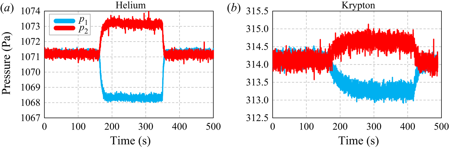
 $^3$, respectively. For the lighter gases, such as helium and neon, this volume configuration could be perfectly used, since the amplitude of the pressure variation in the cold tank is sufficiently high for the whole covered pressure range. However, for heavier gases, such as argon and krypton, the amplitude of pressure variation inside the tanks is considerably lower, mainly for high pressures. In this case, it becomes very difficult to fit the pressure variation in the cold tank with an exponential function because the instantaneous pressure fluctuations start to be very important compared with the pressure variation in time. Figure 8 shows the pressure variation inside the hot and cold tanks for helium (figure 8a) and krypton (figure 8b) considering the same temperature difference and the same level of gas rarefaction. It is clear that the pressure variation inside the cold tank is much higher for helium (
 $\sim$3 Pa) than for krypton (
 $\sim$1 Pa). Consequently, in the case of krypton, the fluctuations of the pressure signal are more significant compared with the total pressure variation in a tank, so it is difficult to fit the pressure behaviour with the exponential function with a good accuracy.
Behaviour of the pressure variation inside the hot and cold tanks in temperature gradient experiments using (a) helium and (b) krypton. The volume ratio, rarefaction parameter and temperature difference between the tanks used in both experiments are  $V_{ratio}=0.678,\ \delta = 10$ and
 $\Delta T=58\,^{\circ }\textrm {C}$, respectively.

To overcome this problem of very small amplitude of the pressure variation in the cold tank, the total volume of the hot side was increased by including an additional reservoir connected to the system by the valve  $V_{R2}$, see figure 1. For this new volume configuration, the increase in the amplitude of the pressure variation in the cold side due to the change of the volume ratio between hot and cold sides can be estimated. As was shown in § 4.1, the amplitude of the pressure variation in each tank is related to the volume of the tanks. However, in the case of the temperature gradient driven flow, (4.7) needs to be modified to take into account of the different temperatures of the tanks, so it becomes
 \begin{equation} \textrm{d} p_1 \frac{V_1}{T_1}={-}\textrm{d} p_2 \frac{V_2}{T_2}. \end{equation}
By integrating this equation between initial,  $t_0$, and final,
 $t_f$, time instants, we have
 \begin{equation} \Delta p_1 =\Delta p_2 \frac{V_2}{V_1}\frac{T_1}{T_2}. \end{equation}
By using (4.17), the amplitude of the pressure variation in the cold tank can be estimated for both volume configurations.
By comparing figures 7(a) and 7(b) it can be observed that the amplitudes of the pressure variation inside the cold and hot tanks are changed when the volume ratio is modified. For the first scenario, figure 7(a), when  $V_1=12.6\ \textrm {cm}^3$ and
 $V_2=18.6\ \textrm {cm}^3$,
 $V_2/V_1=1.476$ and
 $T_1/T_2=0.831$ the amplitude of the pressure variation inside the cold tank is approximately 1.23 times higher than the amplitude of the pressure variation inside the hot tank, i.e.
 $\Delta p_1 \approx 1.23 \Delta p_2$. However, for the second scenario, figure 7(b), where
 $V_1=12.6\ \textrm {cm}^3$ and
 $V_2=75.3\ \textrm {cm}^3$,
 $V_2/V_1=5.976$, the amplitude of the pressure variation inside the cold tank is much higher than the amplitude of pressure variation inside the hot tank, i.e.
 $\Delta p_1 \approx 4.87\Delta p_2$. Therefore, for the second set-up configuration with the highest difference between the volumes, the amplitude of the pressure variation on the cold side increases considerably, reducing consequently the importance of its fluctuations, then increasing the accuracy of exponential fit of the pressure curve. Besides, for the experiments carried out with additional volume at the hot side, the experiment duration increases, since the relaxation time is also increased, i.e. it takes more time to achieve the stabilization of the pressures in both tanks.
During each experiment, which always lasts no longer than 6 min, the temperature is monitored by an IR camera. The mean value of the temperature,  $\overline {T_i}$, and its standard deviation,
 $s_i$, are calculated. As for the pressure driven flows, the ratio
 $s/\overline {T_i}$ is assumed to be a pertinent representation of the temperature variation. The temperature fluctuations in the cold tank are found to be
 $dT_1/T_1\approx 7\times 10^{-5}$, while in the hot tank they are
 $dT_2\approx 6\times 10^{-5}$. On the other hand, the pressure fluctuations on the cold side are higher than those at the hot side and they are in the ranges of
 $0.001< dp_1/p_1<0.03$ and
 $0.0002< dp_2/p_2<0.004$, respectively. Summing up, the temperature fluctuations are relatively small compared with the pressure fluctuations in the cold tank, i.e.
 $\epsilon _1$ is lower than 0.05. However, for the hot tank, the pressure fluctuations are very small, especially for heavier gases, and for these cases,
 $\epsilon _2$ is of the order of 0.30. Therefore, it is not possible to extract the mass flow rate from the pressure measurements in the hot tank (tank 2) using (4.3) (or derived from it under condition of smallness of
 $\epsilon _2$, right-hand side of (4.15a,b)), because
 $\epsilon _2$ is not small enough compared with unity. In the following, only the measurements made on the cold side are presented and analysed.
4.3. Uncertainty measurement of the mass flow rate
The classical uncertainty calculation technique is used to estimate the measurement uncertainty of the mass flow rate when it is calculated from the pressure evolution for both pressure and temperature gradient experiments, (4.10a,b) and (4.14a,b) respectively. The general expression of uncertainty on the mass flow rate measurements reads
 \begin{equation} {\frac{\delta \dot M_i}{\dot M_i} = \frac{\delta V_i}{V_i} + \frac{\delta p_i}{p_i} +\frac{\delta T_i}{T_i} + \frac{\delta \tau}{\tau},} \quad i=1,2. \end{equation}
All the terms presented on the right-hand side of (4.18) are described below and their estimations are given in table 4. As was explained in the previous section, for the temperature gradient experiments, the measurements are carried out on the cold side only.
To measure the uncertainty of the volume  $V_i$,
 $\delta V_i/V_i$, a reference reservoir with known volume is used and the pressure is measured inside this volume (Johansson et al. Reference Johansson, Testa, Zaier, Perrier, Bonnet, Moulin and Graur2018). The volume of the reference reservoir implemented in this procedure has already an uncertainty of approximately 2 %.
Taking into account the uncertainty on the internal volumes of the valves, open and closed during the procedure of the volume  $V_i$ measurement, and the uncertainty of the pressure transducers, the total uncertainty of volume is 3 %.
The uncertainty on the pressure measurements is due to the uncertainty on the pressure sensors. This value is provided by the manufacturer and it varies from 0.2 % to 0.4 %, depending on the sensor type. The uncertainty on the temperature measurements is due to the uncertainty on the thermocouples, which is of the order of 0.3 %, and uncertainty of the IR camera, which is of the order of 0.7 %. As for the mass flow rate extraction, the values of the temperature obtained from the IR camera have been used, being the uncertainty of 0.7 % provided in table 4.
Finally, the uncertainty on the fitting parameter  $\tau$ is obtained from the difference in magnitude of a 95 % confidence interval for
 $\tau$ to represent the experimental data. The value of this uncertainty is higher for temperature gradient experiments, due to the higher ratio between the fluctuation of the pressure signal and the pressure variation in time.
In table 4 we provide also two parameters which are not involved in (4.10a,b) and (4.14a,b) for the mass flow rate determination, but which impact the uncertainty of its calculation. The first quantity is the value of  $\epsilon _i$, which represents the estimation of the non-isothermal effects, see also § 4, (4.3). These
 $\epsilon _i$ terms were neglected when deriving (4.10a,b) and (4.14a,b), therefore they do not appear in (4.18). However, the provision of these terms should give the idea on the accuracy of the model used for the mass flow rate extraction. This is why we included the values of
 $\epsilon _i$ in the total uncertainty on the mass flow rate. Finally, the last source of error in the mass flow rate measurement comes from the leakages,
 $\dot M_{leak}$, mainly through the gap between the microchannel plates. The values of
 $\dot M_{leak}$ are also provided in table 4 and they are included in
 $\delta \dot M_i/ \dot M_i$ calculations.
As can be seen in table 4, the uncertainties of the mass flow rate for pressure gradient experiments are very similar for high pressure and low pressure tanks. In the following, the data coming from the measurements in the low pressure tank are provided. For the temperature gradient experiments only uncertainties for the cold tank are given in table 4, since the pressure variations in the hot tank were very small compared with the initial pressure, especially for the high pressure experiments, which has led to the fact that the  $\epsilon _2$ parameter becomes too high (of the order of 0.3) compared with unity and so cannot be neglected in the expression of mass flow rate ((4.3)), see also the comments in § 4.2.1. In the following, the data measured in the cold tank are used and analysed.
It should be also mentioned that the maximum values of uncertainties are presented in table 4. For example, the uncertainty on the fitting parameter  $\tau$ is higher for heavier gases than for lighter ones, but the value obtained for krypton is provided in table 4. On the other hand, the leakage uncertainties are higher for light gases, thus the uncertainty of helium leakage is provided.
5. Background theory
In this section, firstly, several definitions related to the gas description at a molecular level are introduced. Then, the main relations used in the experimental extraction of the velocity slip, thermal slip and accommodation coefficients in the case of the pressure and temperature gradient flows are presented. A short description of the two gas–surface interaction models, the Maxwell specular-diffuse model (Cercignani Reference Cercignani1975) and the Cercignani–Lampis model (Cercignani & Lampis Reference Cercignani and Lampis1971), may be found in Appendix C.
5.1. General definitions
The mass flow rate through the same rectangular microchannel was obtained from pressure gradient experiments for the Knudsen number range of  $0.0016< K\!n<0.12$, which means for the hydrodynamic and slip flow regimes, and from temperature gradient flows for the Knudsen number range of
 $0.05< Kn<0.45$, which corresponds to the slip and beginning of transitional flow regimes. The Knudsen number is calculated by using the channel height,
 $H$, as the characteristic flow dimension
 \begin{equation} Kn = \frac{\ell}{H}, \end{equation}
where  $\ell$ is the equivalent molecular free path, calculated as
 \begin{equation} \ell = \frac{\mu}{p} \sqrt{2 {\mathcal{R}} T}, \end{equation}
with  $\mu$ the viscosity of the gas, calculated according to following expression (Bird Reference Bird1994):
 \begin{equation} \mu = \mu_{ref} {\left( \frac{T}{T_{ref}} \right)}^\omega, \end{equation}
where  $\mu _{ref}$ is the gas viscosity at reference temperature
 $T_{ref}=273.15\ \textrm {K}$ and
 $\omega$ is the viscosity index. The rarefaction parameter is also used in the following and it is defined as the inverse of the Knudsen number
 \begin{equation} \delta = \frac{H}{\ell}=\frac{1}{Kn}. \end{equation}
5.2. Pressure gradient driven flow
The pressure gradient driven flow through a channel of a rectangular cross-section has been intensively studied in the last decades. Some numerical and analytical results can be found in Sharipov (Reference Sharipov1999a), Graur, Méolans & Zeitoun (Reference Graur, Méolans and Zeitoun2006) and Méolans et al. (Reference Méolans, Nacer, Rojas, Perrier and Graur2012). In our analysis we used the following expression for the mass flow rate obtained from the Stokes equation with the first-order velocity slip boundary condition (Méolans et al. Reference Méolans, Nacer, Rojas, Perrier and Graur2012):
 \begin{equation} \dot M = \dot M{_{{P}}}\left(1+6\sigma_p \frac{T_n}{S_n} Kn\right) , \end{equation}
where  $\dot M {_{{P}}}$ is the Poiseuille mass flow rate, defined as
 \begin{equation} \dot M{_{{P}}} = \frac{H^3 W (1-{\mathcal{K}}) \Delta p p_m}{12 \mu {\mathcal{R}} T L}, \end{equation}
with  $\sigma _p$ the velocity slip coefficient (Albertoni, Cercignani & Gotusso Reference Albertoni, Cercignani and Gotusso1963; Sharipov & Seleznev Reference Sharipov and Seleznev1998) and
 $p_m=(p_1+p_2)/2$ the mean pressure. The coefficient
 $\mathcal {K}$ allows us to take into account the influence of the lateral walls on the Poiseuille mass flow rate, (5.6), and it is obtained from (Sharipov Reference Sharipov1999a; Méolans et al. Reference Méolans, Nacer, Rojas, Perrier and Graur2012)
 \begin{equation} {\mathcal{K}} = 192 \frac{H}{W} \sum_{i=0}^{\infty} \frac{1}{n^5} \tanh \left( \frac{nW}{2H} \right) , \quad n={\rm \pi} (2i+1). \end{equation}
The coefficients  $T_n$ and
 $S_n$ in (5.5) allow us to take into account the influence of the lateral walls on the mass flow rate in slip flow regime and they are calculated from the following expressions (Méolans et al. Reference Méolans, Nacer, Rojas, Perrier and Graur2012):
 \begin{gather} T_n = \frac{4}{3}S_n-\frac{1}{3} \left(1-\frac{H}{W}\right) \sum_{n=0}^{\infty} \frac{\tanh^2 \left(0.5 {\rm \pi}(2n+1)W/H\right)}{(2n+1)^4}, \end{gather}
 \begin{gather} S_n = \frac{{\rm \pi}^4}{96}-\frac{2H}{{\rm \pi} W} \sum_{n=0}^{\infty} \frac{\tanh \left(0.5 {\rm \pi}(2n+1)W/H\right)}{(2n+1)^5}. \end{gather}
It should be mentioned that the equivalent molecular free path,  $\ell$, (5.2), and, consequently, Knudsen number,
 $K\!n$, (5.1), are calculated here using the mean pressure
 $p_m$.
The mass flow rate, (5.5), can be presented also in the dimensionless form
 \begin{equation} S{^{{T}}} = \dot M / \dot M{_{{P}}} = 1+6\sigma_p \frac{S_n}{T_n} Kn=C{^{{T}}}_0+C{^{{T}}}_1Kn, \end{equation}
where
 \begin{equation} C{^{{T}}}_0=1, \quad C{^{{T}}}_1=6\sigma_p \frac{S_n}{T_n}. \end{equation}
We can fit the measured dimensionless mass flow rate analogously to the (5.10) form as a function of Knudsen number
 \begin{equation} S{^{{F}}} =C{^{{F}}}_0+C{^{{F}}}_1Kn, \end{equation}
and then extract the velocity slip from the relation  $C {^{{T}}}_1=C {^{{F}}}_1$, as follows:
 \begin{equation} \sigma_p=\frac{C{^{{F}}}_1}{6} \frac{T_n}{S_n}. \end{equation}
When the velocity slip coefficient for each pair gas–surface is extracted from (5.13), then the accommodation coefficient can be also obtained. The authors of Loyalka, Petrellis & Stvorick (Reference Loyalka, Petrellis and Stvorick1975) calculated the velocity slip coefficient for a given accommodation coefficient using kinetic modelling, namely the Bhatnagar–Gross–Krook (BGK) model, and the Maxwell specular-diffuse scattering kernel. Then, a simple expression associating the slip and accommodation coefficients was proposed
 \begin{equation} \sigma_p (\alpha) = \frac{2-\alpha}{\alpha}(\sigma_p(1) - 0.1211(1-\alpha)) , \end{equation}
where  $\alpha$ is the accommodation coefficient and
 $\sigma _p(1)$ is the slip coefficient for
 $\alpha =1$, with
 $\sigma _p(1)=1.016$ (Albertoni et al. Reference Albertoni, Cercignani and Gotusso1963).
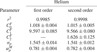
The second-order (in Knudsen number) polynomial fit was used recently by several authors to extract the accommodation coefficient from pressure driven flows (Maurer et al. Reference Maurer, Tabeling, Joseph and Willaime2003; Colin et al. Reference Colin, Lalonde and Caen2004; Graur et al. Reference Graur, Perrier, Ghozlani and Méolans2009; Perrier et al. Reference Perrier, Hadj-Nacer, Méolans and Graur2019). The comparison between the fit of the experimental data of helium to polynomials of first and second orders was carried out in the Knudsen number ranges of  $[0.0016;0.12]$ and
 $[0.0016;0.67]$, respectively. It was found that the difference between the accommodation coefficients derived from the respective fits is of the order of
 $0.1\,\%$, see table 13, so the first-order polynomial fit is used for the coefficient extraction. The values of the velocity slip and accommodation coefficients for each gas–surface pair, obtained for the five analysed gases, are provided in § 6.
5.3. Temperature gradient driven flow
As was underlined in § 4.2, the thermal creep flow is evaluated at instant  $t_0$, where the pressures in both tanks are equal between them and the counterflow from the hot side to the cold has not yet started. At this stage of established thermal creep between two tanks with different temperatures and equal pressures, a very small pressure gradient is generated inside the microchannel (Sharipov Reference Sharipov1999b; Méolans & Graur Reference Méolans and Graur2008; Graur & Ho Reference Graur and Ho2014; Rojas Cárdenas et al. Reference Rojas Cárdenas, Graur, Perrier and Méolans2015; Yamaguchi et al. Reference Yamaguchi, Perrier, Ho, Méolans, Niimi and Graur2016). The total mass flow rate
 $\dot M$ through the channel can be presented as
 \begin{equation} \dot M ={-}\dot M{_{{P}}}+\dot M{_{{T}}}, \end{equation}
where  $\dot M {_{{P}}}$ is the pressure driven flow rate induced by the thermal creep flow and
 $\dot M {_{{T}}}$ is the thermal creep mass flow rate. The pressure profile along the channel has a parabolic shape, with maximum value near to its central point and it was numerically established in Sharipov (Reference Sharipov1999b) and Méolans & Graur (Reference Méolans and Graur2008). Using the previously developed kinetic modelling, the authors of Yamaguchi et al. (Reference Yamaguchi, Perrier, Ho, Méolans, Niimi and Graur2016) estimated the ratio
 $\dot M {_{{P}}}/\dot M$ in the case of very similar temperature gradients and in the case of the flow through a rectangular microchannel to be smaller than 0.2 %. Therefore, the total measured mass flow rate could be identified with a temperature driven mass flow rate as
 \begin{equation} \dot M \approx \dot M{_{{T}}}. \end{equation}
To obtain an explicit expression of the mass flow rate driven by thermal transpiration  $\dot M {_{{T}}}$ in the slip flow regime, the Stokes equation subjected to the thermal slip boundary conditions in the following form
 \begin{equation} u{_{{slip}}}=\sigma{_{{T}}} \frac{\mu}{\rho T}\frac{\textrm{d}T}{\textrm{d}x} \end{equation}
was integrated over the channel cross-section. Then, the mass flow rate reads (Sharipov Reference Sharipov2011; Yamaguchi et al. Reference Yamaguchi, Perrier, Ho, Méolans, Niimi and Graur2016)
 \begin{equation} \dot M{_{{T}}}=\sigma{_{{T}}}HW\frac{\mu}{T}\frac{\textrm{d}T}{\textrm{d}x}. \end{equation}
In previous expressions,  $\sigma {_{{T}}}$ is the thermal slip coefficient (Sharipov Reference Sharipov2011),
 $\rho$ is the gas density and
 $\textrm {d}T/{\textrm {d}x}$ is the temperature gradient along the channel walls in the
 $x$-direction. The thermal slip coefficient could be extracted from (5.18) if the temperature gradient along the channel is known (Yamaguchi et al. Reference Yamaguchi, Perrier, Ho, Méolans, Niimi and Graur2016). However, this is only a first-order solution according to the Knudsen number and it is not accurate enough (Rojas Cárdenas et al. Reference Rojas Cárdenas, Graur, Perrier and Méolans2015; Yamaguchi et al. Reference Yamaguchi, Perrier, Ho, Méolans, Niimi and Graur2016). The higher-order solution for the dimensionless temperature driven mass flow rate between two infinite parallel plates was obtained from the kinetic theory in Loyalka & Hickey (Reference Loyalka and Hickey1989)
 \begin{equation} \dot M{_{{T}}} =HW \frac{ \mu}{T}\frac{\textrm{d}T}{\textrm{d}x} \left({\mathcal{C}}_0{^{{T}}} + \frac{{\mathcal{C}}_1{^{{T}}}}{\delta} + \frac{{\mathcal{C}}_2{^{{T}}}}{\delta^2}+ O \left(\frac{1}{\delta^3}\right)\right), \end{equation}
where the values of the two coefficients  ${\mathcal {C}}_0 {^{{T}}}$ and
 ${\mathcal {C}}_1 {^{{T}}}$ were calculated in Loyalka & Hickey (Reference Loyalka and Hickey1989), being equal to
 ${\mathcal {C}}_0 {^{{T}}}=0.9924$ and
 ${\mathcal {C}}_1 {^{{T}}}=-1.3284$. Following Yamaguchi et al. (Reference Yamaguchi, Perrier, Ho, Méolans, Niimi and Graur2016) and Rojas Cárdenas et al. (Reference Rojas Cárdenas, Graur, Perrier and Méolans2015), we integrated this asymptotic solution, but up to the term of the order of
 $O(1/\delta ^3)$, so the expression for the mass flow rate becomes
 \begin{equation} \dot M{_{{T}}} = \dot M{_{{ref}}} \left({\mathcal{C}}_0{^{{T}}} + \frac{{\mathcal{C}}_1{^{{T}}} {\mathcal{C}}_1'}{\delta{_{{m}}}} + \frac{{\mathcal{C}}_2{^{{T}}} {\mathcal{C}}_2'}{\delta{_{{m}}}^2}+ O \left(\frac{1}{\delta{_{{m}}}^3}\right)\right), \end{equation}
where
 \begin{equation} \dot M{_{{ref}}} = \frac{HW \mu{_{{ref}}}}{T{_{{ref}}}^{\omega}} \frac{T_2^{\omega}-T_1^{\omega}}{\omega L}. \end{equation}
The mean value of the rarefaction parameter,  $\delta {_{{m}}}$, is calculated according to
 \begin{equation} \delta{_{{m}}} = \frac{p_0 H}{\mu(T{_{{m}}}) \sqrt{2 {\mathcal{R}} T{_{{m}}}}}, \end{equation}
where  $T_m=0.5(T_1+T_2)$ is the mean temperature; the viscosity coefficient is calculated also using this mean temperature. The term
 ${\mathcal {C}}_0 {^{{T}}}$ in (5.20) can be identified as the thermal slip coefficient,
 $\sigma {_{{T}}}$. Two additional coefficients come from the integration of (5.19) along the channel and they are equal to
 \begin{equation} {\mathcal{C}}_1' = \frac{T_2^{2\omega+0.5} - T_1^{2\omega+0.5}}{(2\omega+0.5)T_m^{\omega+0.5}}\frac{\omega}{T_2^{\omega}-T_1^{\omega}}, \quad {\mathcal{C}}_2' = \frac{T_2^{3\omega+1} - T_1^{3\omega+1}}{(3\omega+1)T_m^{2\omega+1}}\frac{\omega}{T_2^{\omega}-T_1^{\omega}}. \end{equation}
The values of both coefficients are very close to one with a deviation less than 1 %, so they are assumed to be equal to 1 in the following. Therefore, (5.20) can be rewritten in more convenient form by dividing it by the reference mass flow rate,  $\dot M {_{{ref}}}$, and by neglecting the terms of the order of O(
 $1/\delta {_{{m}}}^3)$
 \begin{equation} {\mathcal{G}}{^{{T}}}= \frac{\dot M{_{{T}}}}{\dot M{_{{ref}}}} = {\mathcal{C}}_0{^{{T}}} + \frac{{\mathcal{C}}_1{^{{T}}}}{\delta{_{{m}}}}+\frac{{\mathcal{C}}_2{^{{T}}}}{\delta{_{{m}}}^2}={\mathcal{C}}_0{^{{T}}} + {\mathcal{C}}_1{^{{T}}}Kn{_{{m}}}+{\mathcal{C}}_2{^{{T}}}Kn{_{{m}}}^2. \end{equation}
As the fit in the polynomial form is more convenient compared with the previous expression, we use the following expression to fit the experimental data
 \begin{equation} {\mathcal{G}}{^{{F}}}(Kn{_{{m}}}) = \frac{\dot M{_{{T}}}}{\dot M{_{{ref}}}} = {\mathcal{C}}_0{^{{F}}} + {\mathcal{C}}_1{^{{F}}}Kn{_{{m}}}+{\mathcal{C}}_2{^{{T}}}Kn{_{{m}}}^2, \end{equation}
in the slip and beginning of transitional flow regimes,  $0.05< Kn {_{{m}}}<0.45$. The fitting coefficient
 ${\mathcal {C}}_0 {^{{F}}}$ is associated with the coefficient
 $\sigma {_{{T}}}$.
Finally, the accommodation coefficient,  $\alpha$, was calculated from the thermal slip coefficient by using the expression proposed in Sharipov (Reference Sharipov2011) and Suetin & Chernyak (Reference Suetin and Chernyak1977) and obtained using the S-model kinetic equation with Maxwellian specular-diffuse boundary condition
 \begin{equation} \sigma_T = 0.75 (1+0.5\alpha). \end{equation}
For the case of a polyatomic gas such as nitrogen, it is necessary to take into account the effects of the internal degrees of freedom of the molecule, as formulated in the expression proposed in Loyalka & Storvick (Reference Loyalka and Storvick1979) and Loyalka, Storvick & Lo (Reference Loyalka, Storvick and Lo1982), where the model of Hanson and Morse was used. Thus the expression of the thermal slip coefficient for a polyatomic gas reads
 \begin{equation} \sigma_T = \tfrac{3}{10}\,f_{tr} (1+0.5\alpha), \end{equation}
where  $\,f_{tr}$ is the translational Eucken factor, which is equal to 2.25 for nitrogen (Porodnov et al. Reference Porodnov, Kulev and Tuchvetov1978).
The thermal slip and accommodation coefficients obtained from temperature gradient driven flow, as well as the fitting coefficients for all the five gases used in the present work (He, Ne, N $_2$, Ar and Kr), are presented in the next section.
6. Results
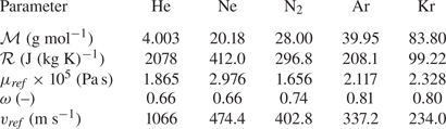
Several important parameters of the five gases used in the experiments are presented in table 5: molar mass ( $\mathcal {M}$), specific gas constant (
 $\mathcal {R}$), reference viscosity (
 $\mu {_{{ref}}}$), viscosity index (
 $\omega$) and reference most probable speed (
 $v {_{{ref}}}$). The reference viscosity and reference most probable speed are given considering the reference temperature,
 $T {_{{ref}}}=273.15\ \textrm {K}$. It should be noticed that the viscosity and viscosity index, provided in table 5, are taken from the widely used Bird (Reference Bird1994). However, more recent data on both quantities are available in Sharipov & Benites (Reference Sharipov and Benites2020) and Xiao et al. (Reference Xiao, Rowland, Al Chafri and May2020).
Characteristic parameters of all five gases used in the experiments.

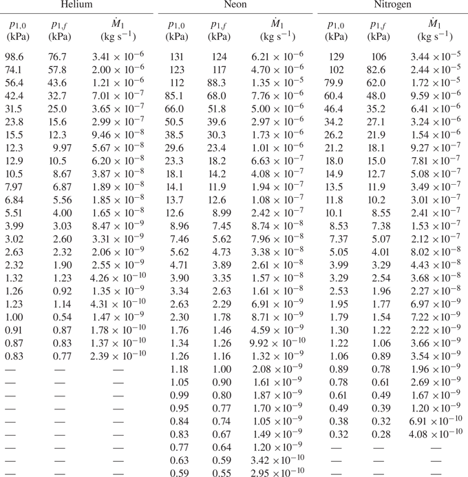
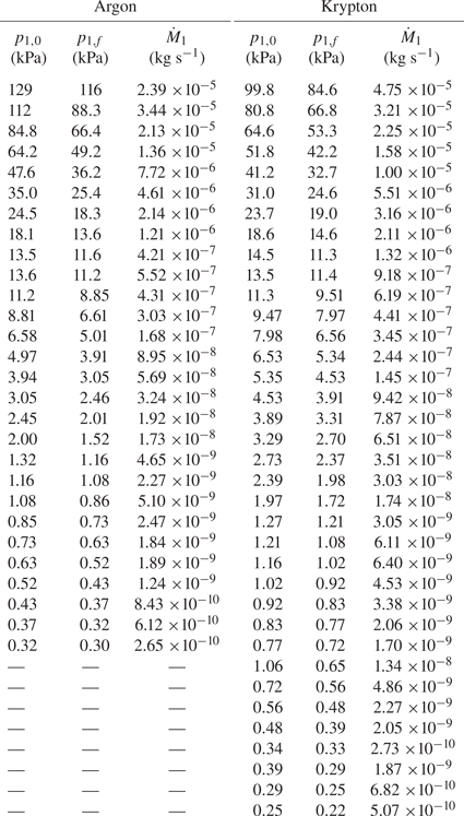
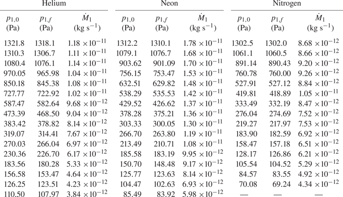
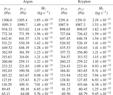
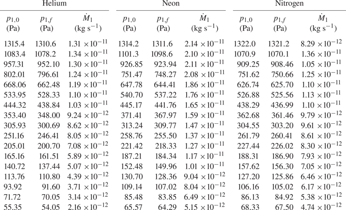
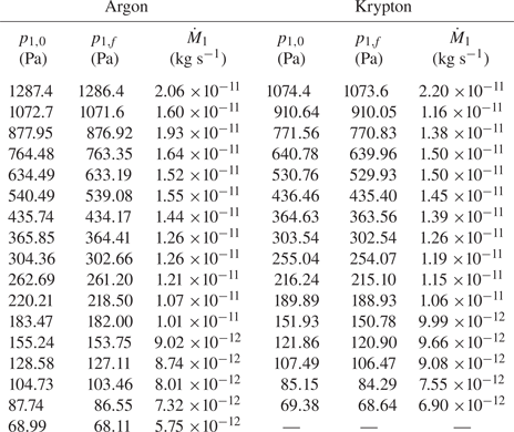
Tables with initial and final pressures in the upstream tank and the mass flow rates extracted from both pressure gradient and temperature gradient driven flows are provided in Appendix D.
6.1. Pressure gradient driven flow
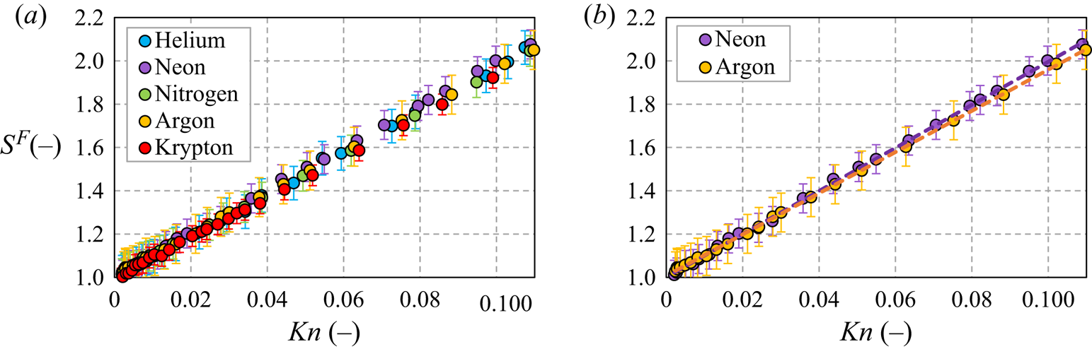
As explained in § 5, the analytical expression of the mass flow rate, (5.5), was obtained from the solution of the Stokes equation subjected to the first-order velocity slip boundary condition. Therefore, the measured mass flow rate was evaluated inside the Knudsen number range of  $0.0016< Kn<0.12$. Figure 9(a) shows the measured dimensionless mass flow rate,
 $S=\dot M / \dot M {_{{P}}}$, as a function of the Knudsen number for all the five gases used in the experiments, while figure 9(b) represents this mass flow rate only for neon and argon, providing also the fitting curves of the affine fitting functions, (5.12), for both gases.
Dimensionless measured mass flow rate,  ${S {^{{F}}}}=\dot M / \dot M {_{{P}}}$, (filled symbols) as a function of the Knudsen number: (a) for all the five gases used in the experiments; (b) for neon and argon with the affine fitting curves (dashed lines).

The fitting parameters,  $C {^{{F}}}_0$ and
 $C {^{{F}}}_1$, and the determination coefficient,
 $r^2$, for all the five gases are presented in table 6. The uncertainty of both fitting coefficients is estimated using the standard error. The experimental uncertainty, provided in table 4, is not added to the adjustment uncertainty. Finally, part of these uncertainties concerns the random uncertainty linked to the pressure and temperature measurements, so the influence of these uncertainties is taken into account by the adjustment procedure. The other part of the systematic uncertainties, such as volume uncertainty, is estimated to be very low. This conclusion could be obtained by analysing the values of the coefficients
 $C_0 ^ {F}$ in table 4. Its values are very close to one, which proves that the measured Poiseuille mass flow rate is obtained with good precision.
Determination coefficient, coefficients of affine fitting, velocity slip and accommodation coefficients obtained from pressure gradient experiments for the five gases.

As can be seen in table 6, the determination coefficient,  $r^2$, is very close to one, indicating that the linear regression fits very well to the measured mass flow rate values for all of the evaluated Knudsen number range. The values of the fitting coefficient
 $C {^{{F}}}_0$ are very close to one (deviation is lower than 2 %) for all of the gases, confirming the good approximation of the Poiseuille mass flow rate (Ewart et al. Reference Ewart, Perrier, Graur and Méolans2007) and therefore small systematic error of the measurements.
The values of the velocity slip coefficient, calculated using (5.13), varies from 1.485 for krypton to 1.584 for neon and they are relatively close one to another for all the analysed gases. These values are far from 1.016, the value theoretically found in Albertoni et al. (Reference Albertoni, Cercignani and Gotusso1963) for the complete accommodation (complete diffuse scattering).
The accommodation coefficients,  $\alpha {_{{p}}} {^{{M}}}$, obtained from (5.14), are also presented in table 6. The subscript ‘
 $p$’ is used to notify that these coefficients are obtained from the pressure driven experiments and the superscript ‘
 $M$’ indicates that the coefficients are extracted using the Maxwell specular-diffuse kernel. The values of the accommodation coefficient,
 $\alpha {_{{p}}} {^{{M}}}$, lie also in the narrow range from 0.768 for neon to 0.801 for krypton. For all gases, except helium, the dependency from the mass is clearly seen: the accommodation coefficient is closer to one for the heavier gases. However, it is difficult to explain why the accommodation coefficient of helium does not follow this trend.
The influence of the surface roughness on the gas–surface interaction has been studied for a long time, nevertheless, up to now there does not exist a common point of view regarding the influence of surface roughness on flow properties; see the review paper Agrawal & Prabhu (Reference Agrawal and Prabhu2008). Generally, an increasing surface roughness leads to an increasing accommodation of the molecules on the surface and therefore to an increase in the value of the accommodation coefficient. However, the authors of Blanchard & Ligrani (Reference Blanchard and Ligrani2007) have made a systematic study of the roughness influence on a PEEK surface (the same as in the present study) and they found that an increasing roughness (from 10 nm to 770 nm) decreases the accommodation coefficient for the two tested gases: helium (from 0.915 to 0.253) and air (from 0.885 to 0.145). The roughness of the channel used in present experimental set-up was measured to be equal to 113nm, so we consider that our data are compatible with study carried out in Blanchard & Ligrani (Reference Blanchard and Ligrani2007). Therefore, the fact that the values of the accommodation coefficients are found to be relatively far from unity could be explained by the influence of the relatively high roughness of the microchannel, grooved in a PEEK plate.
6.2. Temperature gradient driven flow
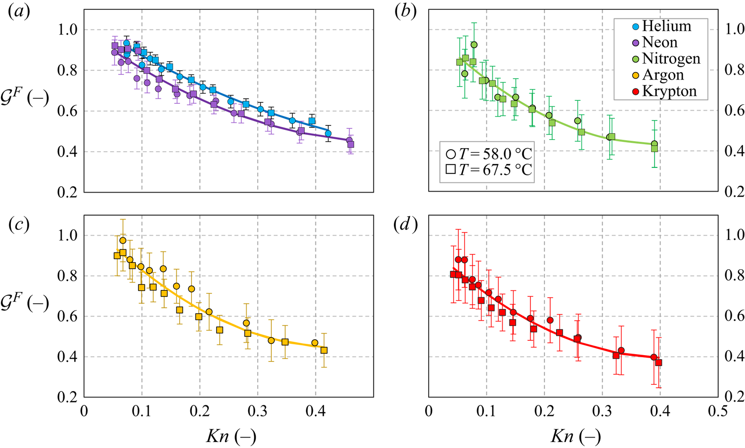
The reduced mass flow rates,  ${\mathcal {G}} {^{{T}}}$, (5.24), for all the five gases (He, Ne, N
 $_2$, Ar and Kr) and for two temperature differences (
 $\Delta T=58.0 \,^{\circ }\textrm {C}$ and
 $67.5 \,^{\circ }\textrm {C}$) are shown in figure 10, as a function of the mean Knudsen number. The fitting curves, (5.25), for each gas are also presented in the same figure. It is important to mention that the fitting curve of each gas was obtained by fitting all the points for each gas, i.e. using both temperatures differences. As we can see in figure 10, the values of
 ${\mathcal {G}} {^{{T}}}$ obtained for helium and neon are almost all over their fitting curves, but if we track
 ${\mathcal {G}} {^{{T}}}$ for the heavier gases, we can see a considerable dispersion, mainly for low values of Knudsen number. Thus, it is extremely challenging to extract the coefficients from temperature driven experiments working with heavy gases.
Fitted reduced mass flow rate ( ${\mathcal {G}} {^{{F}}}$) as a function of the Knudsen number for all the five gases and two temperature differences. Results for (a) helium and neon, (b) nitrogen, (c) argon and (d) krypton. The solid lines represent the fitting curves, (5.25), over both temperature differences for each gas.

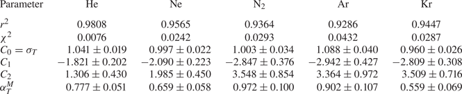
Table 7 presents the values of the fitting coefficients  ${\mathcal {C}} {^{{F}}}_i$,
 $i=0,1$ and 2, with corresponding uncertainties, obtained from the fit of the experimental data, according to (5.25). The
 ${\mathcal {C}} {^{{F}}}_0$ coefficient is associated with the thermal slip coefficient
 $\sigma {_{{T}}}$. The uncertainties of the fitting coefficients provided in table 7 do not consider the uncertainties on the measurements of mass flow rate, but only the standard errors on the fitting process. In addition, to estimate the quality of the fit, two characteristic parameters are also provided: the determination coefficient
 $r^2$ and the
 $\chi ^2$ value. By analysing these two parameters, one can observe that, for the two lighter gases, namely helium and neon, both characteristics are good. For helium, the determination coefficient
 $r^2$ is close to 1 (0.9808) and the probability that the two fitted variables are independent is very small (0.0076). However, for the heavier gases, both characteristic parameters present worse values, especially for argon.
The fitting parameters  ${\mathcal {C}} {^{{F}}}_i$,
 $i=0,1$ and 2, obtained from the fit of the temperature gradient driven mass flow rate for all the five gases. The
 ${\mathcal {C}} {^{{F}}}_0$ coefficient is associated with
 $\sigma {_{{T}}}$. The determination coefficient,
 $r^2$ and the
 $\chi ^2$ probability of the fitting variables to== being independent are provided. The accommodation coefficients extracted from (5.26) and (5.27) in the frame of the Maxwellian kernel are also given.

Table 8 provides the  $\sigma {_{{T}}}$ coefficients previously measured by other authors (Porodnov et al. Reference Porodnov, Kulev and Tuchvetov1978; Rojas Cárdenas et al. Reference Rojas Cárdenas, Graur, Perrier and Méolans2015; Yamaguchi et al. Reference Yamaguchi, Perrier, Ho, Méolans, Niimi and Graur2016) and the values found in present work. If comparing the later values of
 $\sigma {_{{T}}}$ coefficients for monoatomic gases with those from Yamaguchi et al. (Reference Yamaguchi, Perrier, Ho, Méolans, Niimi and Graur2016) obtained using a channel also made by PEEK, one can see that the values obtained here are slightly higher for helium and argon, very similar (but lower) for neon and essentially lower for krypton, compared with those obtained in Yamaguchi et al. (Reference Yamaguchi, Perrier, Ho, Méolans, Niimi and Graur2016). It is worth noting that the roughness of the PEEK surface used here is relatively high, which could impact the values of the
 $\sigma {_{{T}}}$ coefficients, as was observed for the pressure driven flows. The
 $\sigma {_{{T}}}$ coefficient of the polyatomic nitrogen is found to be the highest one compared with those given in previously reported articles (Porodnov et al. Reference Porodnov, Kulev and Tuchvetov1978; Rojas Cárdenas et al. Reference Rojas Cárdenas, Graur, Perrier and Méolans2015; Yamaguchi et al. Reference Yamaguchi, Perrier, Ho, Méolans, Niimi and Graur2016). No correlation of these values with the molecular weight of the gas was found.
The  $\sigma _T$ coefficient obtained in the present work and by the authors of Porodnov et al. (Reference Porodnov, Kulev and Tuchvetov1978), Yamaguchi et al. (Reference Yamaguchi, Perrier, Ho, Méolans, Niimi and Graur2016) and Rojas Cárdenas et al. (Reference Rojas Cárdenas, Graur, Perrier and Méolans2015). The authors of Yamaguchi et al. (Reference Yamaguchi, Perrier, Ho, Méolans, Niimi and Graur2016) used a microchannel made by PEEK (same material as in the present experiments), while in Porodnov et al. (Reference Porodnov, Kulev and Tuchvetov1978) and Rojas Cárdenas et al. (Reference Rojas Cárdenas, Graur, Perrier and Méolans2015) microchannels made from glass are considered.

By fitting the temperature driven mass flow rate in the second-order polynomial form, we associate the thermal slip coefficient with zero order in the Knudsen number term. However, this term is very difficult to fix, because we need to have more data for very small Knudsen number, which are difficult to obtain. Let us now analyse the ‘second thermal slip coefficient’,  ${\mathcal {C}}_1$ coefficient in (5.19). Analysing the values of this coefficient, all gases can be separated into two groups: the two lighter gases (helium and neon) for which the second slip coefficients,
 ${\mathcal {C}}_1$, have similar values,
 $-1.821$ and
 $-2.090$, respectively; heavier gases, nitrogen, argon and krypton, for which this second slip coefficient has also similar values,
 $-2.847$,
 $-2.942$ and
 $-2.809$, respectively, see also table 7. The analytical value of this second slip coefficient,
 ${\mathcal {C}}_1=-1.3284$, was provided in Loyalka & Hickey (Reference Loyalka and Hickey1989) for the case of two parallel plates and Maxwell diffuse scattering. This analytical value has the same sign, but much smaller absolute value as those obtained from the fits of the experimental data.
The accommodation coefficients,  $\alpha {^{{M}}} {_{{T}}}$, obtained from the thermal slip coefficients by using (5.26) and (5.27), are given in table 7. The subscript ‘
 $T$’ is used to notify that these coefficients are obtained from the temperature gradient experiments and the superscript ‘
 $M$’ indicates that the coefficients are extracted using the Maxwell specular-diffuse kernel. The values of
 $\alpha {^{{M}}} {_{{T}}}$ vary in a large range, with a minimum value of 0.559 for krypton and maximum value of 0.972 for nitrogen. As the accommodation coefficient is extracted from the thermal slip coefficient, using (5.26) and (5.27), the uncertainties on
 $\alpha$ represent 8/3 of the uncertainties on
 $\sigma {_{{T}}}$ for all monoatomic gases and 80/27 for nitrogen. Both latter quantities were obtained by classical derivation rule, which allows us to calculate the uncertainties. It is clear from table 7 that, for heavier gases, the uncertainties on the accommodation coefficients are larger than that for helium and neon, which could be explained by more scattered
 ${\mathcal {G} {^{{T}}}}$ values for heavier gases.
6.3. Comparison between accommodation coefficients
The values of accommodation coefficient obtained from pressure ( $\alpha {^{{M}}} {_{{P}}}$) and temperature (
 $\alpha {^{{M}}} {_{{T}}}$) gradient experiments are summarized in table 9. As previously mentioned, the superscript ‘
 $M$’ denotes that the Maxwellian specular-diffuse model was used for the extraction of these coefficients. Analysing table 9, we can conclude that the values of all accommodation coefficients obtained from pressure gradient experiments are close to each other with the difference between minimal (neon) and maximal (krypton) values of the order of 4 %. Moreover, for the accommodation coefficients extracted from temperature gradient experiments, the difference is much higher, being of the order of 42 %. Besides, only for helium are the two coefficients, obtained from the pressure and temperature gradient experiments, very close to each other, with 0.5 % of difference. For all the other gases, this difference varies between 12 % (argon) and 30 % (krypton). Therefore, the question remains open as to which coefficient should be used in numerical simulations when both pressure and temperature gradients are present in a flow and Maxwellian boundary conditions are used. To go forward in answering this question, numerical studies need to be carried out to conclude on the choice of the coefficients. In the frame of continuum simulations (Navier–Stokes–Fourier equations), different possibilities exist, as, for example, to put the
 $\alpha {^{{M}}} {_{{P}}}$ in the velocity slip boundary conditions and
 $\alpha {^{{M}}} {_{{T}}}$ in the thermal slip part. However, if the Maxwell kernel is used in the frame of kinetic equation, a real choice has to be made because only one coefficient is used in the boundary conditions.
Accommodation coefficients extracted from both pressure and temperature driven flows,  $\alpha {^{{M}}} {_{{P}}}$ and
 $\alpha {^{{M}}} {_{{T}}}$, respectively, in the frame of the Maxwellian model.

A more sophisticated model can also be applied to take into account simultaneously the influence of both momentum and energy exchanges, through two different accommodation coefficients, i.e. considering a tangential momentum accommodation coefficient, $\alpha _t$, and normal energy accommodation coefficient,
 $\alpha _n$, (Cercignani & Lampis Reference Cercignani and Lampis1971). The extraction of both coefficients in the frame of the Cercignani–Lampis model (Cercignani & Lampis Reference Cercignani and Lampis1971) is presented in the next section.
6.4. Accommodation coefficients from Cercignani–Lampis model
The Cercignani–Lampis model was implemented by the authors of Siewert & Sharipov (Reference Siewert and Sharipov2002) andSharipov (Reference Sharipov2003) in the frame of the S-model kinetic equation, while the author of Siewert (Reference Siewert2003) solved directly the Boltzmann equation with a hard-sphere model to study the influence of both the tangential momentum and normal energy accommodation coefficients on the velocity slip coefficient,  $\sigma {_{{p}}}$. From these works it was concluded that this coefficient is weakly affected by the normal energy accommodation coefficient,
 $\alpha _n$, but it significantly depends on the tangential momentum accommodation coefficient,
 $\alpha _t$. The expression relating
 $\sigma {_{{p}}}$ and
 $\alpha _t$, which interpolates the numerical results obtained by the authors, is
 \begin{equation} \sigma{_{{p}}} = \frac{1.771}{\alpha_t}-0.754. \end{equation}
Thus, the first adjustable parameter of the Cercignani–Lampis model,  $\alpha _t$, depends only on
 $\sigma {_{{p}}}$, and this last coefficient comes from the pressure gradient experiments. Therefore, from the already extracted velocity slip coefficients, see table 6, the tangential momentum accommodation coefficient,
 $\alpha _t$, is obtained and its values are provided in table 10. It should be mentioned that the values of accommodation coefficient obtained using the specular-diffuse model,
 $\alpha {^{{M}}} {_{{p}}}$, are also shown in this table in order to facilitate the comparison with
 $\alpha _t$.
Velocity slip and accommodation coefficients experimentally obtained from pressure gradient experiments for five gases. Maxwellian specular-diffuse model is used to extract  $\alpha {_{{p}}} {^{{M}}}$, while the Cercignani–Lampis one is used to obtain
 $\alpha _t$.

From table 10, it is clear that the values of  $\alpha _t$ vary inside a narrow range between 0.758 for neon and 0.791 for krypton. Comparing the results from both models, it is noticeable that the values of the accommodation coefficient extracted from Cercignani–Lampis model are slightly lower (with maximal difference of 1.3 %) than the values obtained from Maxwellian model, for all the five tested gases.
According to the results provided in Sharipov (Reference Sharipov2011), the thermal slip coefficient,  $\sigma {_{{T}}}$, is sensitive to both accommodation coefficients,
 $\alpha _t$ and
 $\alpha _n$. Thus, if the values of
 $\alpha _t$ and
 $\sigma {_{{T}}}$ are known, the value of the normal energy accommodation coefficient can be obtained. Unfortunately, we did not find in the open literature any explicit expression analogous to, for example, (6.1), to relate the thermal slip coefficient,
 $\sigma {_{{T}}}$, to both accommodation coefficients,
 $\alpha _t$ and
 $\alpha _n$. Therefore, we used a table from Sharipov (Reference Sharipov2011), reproduced below as table 11, to evaluate the behaviour of the
 $\alpha _n$ coefficient.
Thermal slip coefficient  $\sigma {_{{T}}}$ for Cercignani–Lampis scattering law: (a) Siewert & Sharipov (Reference Siewert and Sharipov2002) and Sharipov (Reference Sharipov2003), S model, direct solution; (b) Siewert (Reference Siewert2003), Boltzmann equation with the hard sphere model, direct solution. Reproduced from Sharipov (Reference Sharipov2011).

In fact, the values of  $\alpha _t$ and
 $\sigma {_{{T}}}$ are known and they can be seen in tables 10 and 7, respectively. Based on this, normally it would be easy to extract the values of normal energy accommodation coefficient,
 $\alpha _n$, from table 11. As can be seen in table 10, the values of the tangential momentum accommodation coefficient,
 $\alpha _t$, extracted for all the gases, are inside a narrow range from 0.758 to 0.791, which is close to 0.75, the value provided in table 11, see the bold row. However, the implementation of a simple affine interpolation formula obtained from available values of
 $\sigma {_{{T}}}$ and corresponding
 $\alpha _n$ either from Siewert & Sharipov (Reference Siewert and Sharipov2002) and Sharipov (Reference Sharipov2003), columns (a) or from Siewert (Reference Siewert2003), columns (b) in table 11, does not allow us to obtain reasonable values of
 $\alpha _n$. One of the reasons for that could be the use of an approximate value of
 $\alpha _t=0.75$ instead of a real measured value. Another reason is also the fact that the value band of the measured values of
 $\sigma {_{{T}}}$ (between 0.960 and 1.088, table 7) is greater than the theoretical band (between 0.964 and 1.019, columns (b) of table 11), therefore, it is impossible to find a unique match between the two sets of data. A lack of numerical data relating
 $\sigma {_{{T}}}$ and
 $\alpha _n$, namely values of
 $\alpha _n$ lower than 0.25, and also a possible nonlinear dependency of
 $\sigma {_{{T}}}$ from
 $\alpha _n$ in this range could be other reasons. In principle, by using the numerical approaches proposed in Siewert & Sharipov (Reference Siewert and Sharipov2002), Sharipov (Reference Sharipov2003) and Siewert (Reference Siewert2003) more data on
 $\sigma {_{{T}}}$ and
 $\alpha _n$ could be obtained. After that, it would be possible to extract
 $\alpha _n$ from experimental data.
Recently, the authors of Nguyen et al. (Reference Nguyen, Graur, Perrier and Lorenzani2020) applied a variational method to solve the Boltzmann equation based on the true linearized collision operator for hard-sphere molecules and the Cercignani–Lampis boundary conditions. Then, an explicit relation between the first- and second-order thermal slip coefficients (our  ${\mathcal {C}}_0$ and
 ${\mathcal {C}}_1$ coefficients in (5.25)) and the tangential momentum and normal energy accommodation coefficients, defined in the frame of the Cercignani–Lampis scattering kernel, are derived. By comparing the theoretical results with the experimental data from Yamaguchi et al. (Reference Yamaguchi, Perrier, Ho, Méolans, Niimi and Graur2016), a pair of accommodation coefficients has been extracted for each noble gas considered in the experiments. The approach developed in Nguyen et al. (Reference Nguyen, Graur, Perrier and Lorenzani2020) cannot be applied directly to the present experimental data because the two parallel plate configuration is considered and so the influence of the vertical channel walls is not taken into account. It is worth underlining that the authors of Nguyen et al. (Reference Nguyen, Graur, Perrier and Lorenzani2020) have found the tangential momentum accommodation coefficient in a very narrow range of
 $0.80<\alpha _t<0.88$, not far from our finding, but the normal energy accommodation coefficient was found to be very low, between 0.15 and 0.33. This fact coincides with our previous discussion on the necessity of additional data in the low range of
 $\alpha _n$.
It is worth adding that the authors of Nguyen et al. (Reference Nguyen, Graur, Perrier and Lorenzani2020) have found, by analysing the experimental data of Yamaguchi et al. (Reference Yamaguchi, Perrier, Ho, Méolans, Niimi and Graur2016), that the second thermal slip coefficient is proportional to the molecular mass of a gas: the smallest in absolute value second-order thermal slip coefficient was found for helium and the largest for krypton. Similar behaviour was found from the fit of the present experimental data, see table 7.
7. Conclusion
Two types of gas flow through the same microchannel made from PEEK were experimentally studied. In the first case, the flow is generated by applying a pressure difference between the two sides of the microchannel, while in the second one, the flow is generated by a temperature difference imposed between the two extremities of the microchannel. In both experiments, the pressure variations inside the tanks connected by the microchannel allow us to obtain the mass flow rate through it. Two important parameters characterizing the gas–surface interaction were calculated from these mass flow rates: the velocity slip and the thermal slip coefficients. They are indispensable to simulate gas flows in the slip flow regime in the frame of the continuum approach. For the first time these data were obtained for the same gas–surface pair.
As both velocity and thermal slip coefficients are related to one (Maxwell model) or two (Cercignani–Lampis model) accommodation coefficients, their values were also extracted. Assuming first the hypothesis of the Maxwellian specular-diffuse interaction, where only one coefficient is used for both types of accommodation (tangential momentum and normal energy), the accommodation coefficient of each gas–surface pair was extracted separately from the pressure gradient flows and from the temperature gradient flows. These accommodation coefficients were found to be different when obtained from temperature gradient flows in comparison with the pressure gradient ones, except for helium, for which both coefficients presented very close values, 0.5 % difference.
Applying then the Cercignani–Lampis model, the values of tangential momentum accommodation coefficient obtained from pressure gradient experiments were found to be very close to those previously extracted using the Maxwellian model, with the discrepancy being lower than 1.3 %. However, it was not possible to extract the normal energy accommodation coefficient from the temperature gradient flows due to a lack of numerical data which relate the thermal slip coefficient to the normal energy accommodation coefficient. The extrapolation of the numerical data was also not possible to do, since the behaviour of the thermal slip coefficient as a function of the normal energy accommodation coefficient for the missing range could be different compared with the available one. When these data are available in the open literature, the normal energy accommodation coefficient could also be extracted from the presented measurements.
Finally, the obtained set of experimental data could be useful for numerical modelling of the gas–surface interaction. However, new numerical simulations have to be done to test the capacity of the experimentally extracted coefficients to predict the behaviour of the pressure and temperature gradient flows at small scales or at low pressures.
Acknowledgements
The authors would like to tank N. Ehret for technical and scientific supply in thermal and roughness measurements and Y. Jobic for his help in the experimental data treatment.
Funding
The authors would like to acknowledge financial supports provided by the European Union network program H2020, MIGRATE project under Grant Agreement No.643095.
Declaration of interests
The authors report no conflict of interest.
Appendix A. Non-isothermal effects and their estimation
The non-isothermal effects could be observed after the quick opening and closing of valve  $V_A$. To avoid the non-isothermal measurements, we have proceeded in the following way. Initially, the system is in equilibrium and
 $p_1 = p_2$, see figure 11 interval ‘a’. Then, at time
 $t {_{{i}}}$, the pressure relaxation is actuated by a rapid opening and closing of the valve connected to one of the tanks, where pressure
 $p_2$ is measured. Right after the opening and closing of valve
 $V_A$ (interval ‘b’ in figure 11), the pressure relaxation may be in non-equilibrium and not yet in quasi-equilibrium state. In the non-equilibrium state, we may have a small temperature drop on the low pressure side due to the pressure drop before the system reaches thermal equilibrium again, see figure 11. Therefore, we set a larger pressure ratio than we intend to measure and cut away the first part of the pressure relaxation process, the interval represented by ‘b’ in figure 11. Then, from time instant
 $t_0$, the system reaches the quasi-stationary state, where there is still a pressure change in time. Finally, the final pressure equilibrium is reached,
 $p_1 = p_2$, interval ‘d’, but with one single relaxation time. This range of the quasi-stationary relaxation process, interval ‘c’ in figure 11, is used for the data fitting. We should mention that figure 11 represents a simplified scheme of the whole process. Furthermore, there is an exaggeration in the duration of the non-equilibrium interval, in order to better illustrate the process.
Illustration of typical stages of pressure evolution in time. The red and blue curves represent the pressure variation in the low and high pressure reservoirs, respectively.

In our experimental set-up only the tank temperature is measured. To have an estimation of the time scale of the thermal effects related to the quick opening and closing of the valve  $V {_{{A}}}$, we compare the time needed for a gas to reach equilibrium with the tank, approximately 4
 $\tau {_{{c}}}$ (
 $\tau {_{{c}}}$ is the gas conduction time) (Arkilic et al. Reference Arkilic, Schmidt and Breuer1997) to the waiting time
 $t {_{{w}}}=t_0-t {_{{i}}}$. This latter time represents the time to be waited before starting the measurements.
If the tank represents an infinite heat sink at constant temperature to the gas, then the time it takes for the gas to reach equilibrium with the tank can be modelled. In Arkilic et al. (Reference Arkilic, Schmidt and Breuer1997), the transient heat conduction equation was solved analytically and the solution was presented as an infinite series of Bessel functions. When keeping only the first leading term of the series, the characteristic conduction time can be estimated as
 \begin{equation} \tau{_{{c}}}=\frac{\rho R_{res}^2 Pr}{2.4\mu}, \end{equation}
where  $\rho$ is the gas density,
 $R_{res}$ is the characteristic reservoir dimension and
 $Pr$ is the Prandtl number. In our set-up, the reservoir characteristic dimension (its radius) is equal to 3 mm, the Prandtl number is equal to
 $2/3$ and
 $0.71$, for the monoatomic and polyatomic gases, respectively. The gas conduction time, (A1), is proportional to the gas density and so to the gas pressure under our experimental conditions. It depends also on the nature of the gas through the gas viscosity. As the characteristic conduction time is proportional to the gas density, it is longer for the higher pressure (density) experimental runs. Therefore, we provide the values of
 $\tau {_{{c}}}$ in table 12 only for the high pressure runs. The minimum values of the waiting time are also provided in table 12. The results given in this table provide the experimental confirmation that the gas temperature remains close to a constant temperature during the measurements and that the thermal effects remain negligible under our experimental conditions.
The gas conduction time  $\tau {_{{c}}}$ and the waiting time
 $t {_{{w}}}$ for the high pressure runs for all gases used in experiments.

Appendix B. First- and second-order fittings for pressure driven flows
The pertinence of using the first- or second-order fitting was discussed by different authors, see for example Colin et al. (Reference Colin, Lalonde and Caen2004), Ewart et al. (Reference Ewart, Perrier, Graur and Méolans2007), Maurer et al. (Reference Maurer, Tabeling, Joseph and Willaime2003) and Perrier et al. (Reference Perrier, Hadj-Nacer, Méolans and Graur2019). It was found that the implementation of the second-order fitting formula provides practically the same results as those given by the first-order fitting in corresponding Knudsen number ranges, see table 13.
Determination coefficient, first- and second-order polynomial fitting coefficients, velocity slip and accommodation coefficients obtained from pressure gradient experiments for helium in the range of  $[0.0016;0.12]$ and
 $[0.0016;0.67]$ for the first and second order, respectively.

Appendix C. Gas–surface interaction
As was mentioned in Introduction, the gas–surface interaction becomes very important when the number of molecule–molecule collisions starts to be comparable to the number of molecule–surface collisions. When the gas behaviour is described in terms of the molecular velocity distribution function, the so-called scattering kernel needs to be defined to provide a detailed description of this interaction, i.e. for each known incident distribution function, the reflected distribution function can be calculated. However, in practice, we do not need so detailed a description and the average over molecular velocity characteristics, i.e. the accommodation coefficient, can be used. The accommodation coefficient can be defined as (Sharipov Reference Sharipov2016)
 \begin{equation} \alpha (\psi)=\frac{\textrm{J}{_{{i}}}(\psi)-\textrm{J}{_{{r}}}(\psi)}{\textrm{J}{_{{i}}}(\psi)-\textrm{J}{_{{dif}}}(\psi)}, \end{equation}
where  $\textrm {J} {_{{i}}}(\psi )$ and
 $\textrm {J} {_{{r}}}(\psi )$ are incident and reflected fluxes defined as
 \begin{equation} \textrm{J}{_{{r}}}(\ psi)=\int_{v_n>0} |v_n|\,f({\boldsymbol v}) \psi({\boldsymbol v}) \mbox{d} {\boldsymbol v}, \quad \textrm{J}{_{{i}}}(\psi)=\int_{v_n'<0} |v_n'|\,f({\boldsymbol v}') \psi({\boldsymbol v}') \mbox{d} {\boldsymbol v}', \end{equation}
the diffuse flux is calculated using the Maxwellian distribution function  $f {^{{M}}}$ (Cercignani Reference Cercignani1975) as
 \begin{equation} \textrm{J}{_{{dif}}}(\psi)=\int_{v_n>0} |v_n|\,f^M({\boldsymbol v}) \psi({\boldsymbol v}) \,\mbox{d} {\boldsymbol v}. \end{equation}
In previous equations,  $v_n'$ and
 $v_n$ are the normal components of the incident and reflected molecular velocities and the
 $\psi$ function can present either momentum accommodation,
 $\psi =m {\boldsymbol v}$, or energy accommodation,
 $\psi =m v^2/2$. From the previous definition it is clear that the accommodation coefficient is an integral characteristic (over molecular velocities) and it does not reflect details of the gas–surface interaction.
If the accommodation coefficient is calculated taking  $\psi =mv_t$, where v t is the tangential velocity component of the incident molecule, it is usually called the tangential momentum accommodation coefficient. When using
 $\psi =m v^2/2$ in (C1), the accommodation coefficient becomes the energy (or thermal) accommodation coefficient. In the frame of the Cercignani–Lampis model, the normal energy accommodation coefficient is defined using
 $\psi = mv_n^2/2$.
For some particular kernels, as Maxwellian specular-diffuse and Cercignani–Lampis ones, (C1) does not depend on the molecular velocity distribution function. When using the specular-diffuse scattering,  $\alpha (\psi )=\alpha {_{{d}}}$ for any
 $\psi$ function (Sharipov Reference Sharipov2016). This is the main shortcoming of the specular-diffuse kernel, because it does not allow us to distinguish the tangential momentum and energy accommodation coefficients, by associating both of them with only one coefficient. Contrarily, when using
 $\psi =mv_t$ with the Cercignani–Lampis kernel, one obtains
 $\alpha (\psi )=\alpha _t$, with a meaning of the accommodation of the tangential momentum. In the same way, by using
 $\psi = mv_n^2/2$, the normal energy accommodation coefficient,
 $\alpha (\psi )=\alpha _n$ is obtained.
However, in practice, it is not easy to measure the values of accommodation coefficients for the pairs of the gas–surface interactions, because only the indirect measurements of the macroscopic quantities are available (Saxena & Joshi Reference Saxena and Joshi1981, Reference Saxena and Joshi1989; Agrawal & Prabhu Reference Agrawal and Prabhu2008). The most accurate data can be obtained from simulations based on the kinetic theory, by applying the Boltzmann or other model equations, but the analytical expressions exist usually only in the case of the free molecular flow regime (molecule–molecule collisions are neglected). Contrarily, in the case of the continuum approach, the explicit expressions are available in the case of flow through channels with different cross-sections. When continuum modelling is used, the interaction between a gas and a surface is taken into account through the velocity slip and thermal slip coefficients, which are related to the accommodation coefficients (Sharipov Reference Sharipov2011).
Appendix D. Experimental data
In this section we provide the mass flow through the microchannel for all the five working gases extracted from pressure gradient, tables 14 and 15, and temperature gradient experiments, tables 16–19. It should be noticed that, associated with each mass flow rate are the initial and final pressures inside the upstream tank (tank 1), used to extract this mass flow rate values.
Mass flow rate ( $\dot M_1$) obtained as a function of the initial and final pressures inside the upstream tank (
 $p_{1,0}$ and
 $p_{1,f}$, respectively) extracted for helium, neon and nitrogen from pressure gradient experiments. Both upstream and downstream tanks were kept at
 $24\,^{\circ }\textrm {C}$ during the measurements.

Mass flow rate ( $\dot M_1$) obtained as a function of the initial and final pressures inside the upstream tank (
 $p_{1,0}$ and
 $p_{1,f}$, respectively) extracted for argon and krypton from pressure gradient experiments. Both upstream and downstream tanks were kept at
 $24\,^{\circ } \textrm {C}$ during the measurements.

Mass flow rate ( $\dot M_1$) obtained as a function of the initial and final pressures inside the upstream tank (
 $p_{1,0}$ and
 $p_{1,f}$, respectively) extracted for helium, neon and nitrogen from temperature gradient experiments using
 $\Delta T=58.0\, ^{\circ }\textrm {C}$. During all these measurements, the cold tank was kept at
 $11.5\,^{\circ }\textrm {C}$ and the hot tank at
 $69.5\,^{\circ }\textrm {C}$.

Mass flow rate ( $\dot M_1$) obtained as a function of the initial and final pressures inside the upstream tank (
 $p_{1,0}$ and
 $p_{1,f}$, respectively) extracted for argon and krypton from temperature gradient experiments using
 $\Delta T=58.0\, ^{\circ } \textrm {C}$. During all these measurements, the cold tank was kept at
 $11.5\,^{\circ } \textrm {C}$ and the hot tank at
 $69.5\,^{\circ } \textrm {C}$.

Mass flow rate ( $\dot M_1$) obtained as a function of the initial and final pressures inside the upstream tank (
 $p_{1,0}$ and
 $p_{1,f}$, respectively) extracted for helium, neon and nitrogen from temperature gradient experiments using
 $\Delta T=67.5\, ^{\circ }\textrm {C}$. During all these measurements, the cold tank was kept at
 $11.5\,^{\circ } \textrm {C}$ and the hot tank at
 $79.0\,^{\circ } \textrm {C}$.

Mass flow rate ( $\dot M_1$) obtained as a function of the initial and final pressures inside the upstream tank (
 $p_{1,0}$ and
 $p_{1,f}$, respectively) extracted for argon and krypton from temperature gradient experiments using
 $\Delta T=67.5\, ^{\circ }\textrm {C}$. During all these measurements, the cold tank was kept at
 $11.5\,^{\circ } \textrm {C}$ and the hot tank at
 $79.0\,^{\circ } \textrm {C}$.