1. Introduction
In general, particle simulation models can be grouped into three categories, the particle–particle (PP) model, the particle–mesh (PM) model and the particle–particle particle–mesh (PPPM) model (Hockney & Eastwood Reference Hockney and Eastwood1981). Among these three models, the PP model has the highest accuracy in principle, since it considers the forces of all the pairs of particles. However, the trade-off of high accuracy is the large computational cost, because the number of operations is proportional to the square of the number of particles. This obvious disadvantage prevents the PP model from being widely used in many applications of particle simulations.
In the area of electrostatic plasma simulations, for collisionless plasmas, the well developed and commonly used PM model particle-in-cell (PIC) (Birdsall & Langdon Reference Birdsall and Langdon1991) has succeeded in numerous applications, which not only utilizes a mesh system to reduce the computational cost, but also introduces the concept of a macroparticle to decrease the simulated number of particles and screen out the less interesting short-range particle interactions. For collisional plasmas, however, short-range interactions play a major role, the nature of PIC or other PM models, that particle interactions cannot be resolved within the range of a cell, makes it unsuitable or even unable to capture the correct physics of collisions. Although some other schemes can be added into PIC to consider collisions, such as Monte Carlo binary collision methods (Nanbu Reference Nanbu1997), uncertainties remain in the accuracy of collisions, e.g. how to choose an appropriate Coulomb logarithm. For example, in the regime of small angle scattering, the Coulomb logarithm ($\ln \varLambda \gg 1$ ) could be calculated using the simple formula $\varLambda = \lambda _D / b_{\min }$
 , where $\lambda _D$
 is the Debye length and $b_{\min }$
 denotes a minimum impact parameter. For strongly coupled plasmas, possible large angle scattering exists, the Coulomb logarithm would have to be determined using other theories, as in Ramazanov & Kodanova (Reference Ramazanov and Kodanova2001), where higher-order many-particle correlations are taken into account. To compute collisions accurately and directly without utilizing the Coulomb logarithm, a PP or PPPM (Dimonte & Daligault Reference Dimonte and Daligault2008) model is needed, and except for the large computational cost, simulations using the PP model with real particles (instead of macroparticles) should produce the most trustable results, because the PP model can solve collisions in a desired accuracy given a small enough time step, and it considers all particle correlation effects intrinsically, while PM or PPPM models do not.
For the large computational cost of the PP model, we may not be able to overcome it easily, but with the development of supercomputers and parallel computing techniques, the computational time can be reduced to an amount that is acceptable for simulations on a small spatial scale with a small number of plasma particles. Recent works have already shown that the PP model is feasible for contributing to real applications that require high accuracy of collisions, e.g. electron–ion temperature relaxation problems occurred in inertial confinement fusion (Zhao Reference Zhao2017, Reference Zhao2018a,Reference Zhaob); calculations of conductivity and diffusion coefficients in ultracold plasmas (Bobrov et al. Reference Bobrov, Bronin, Zelener, Zelener, Manykin and Khikhlukha2011; Bobrov, Vorob'ev & Zelener Reference Bobrov, Vorob'ev and Zelener2018; Bobrov et al. Reference Bobrov, Bunkov, Bronin, Klyarfeld, Zelener and Zelener2019, Reference Bobrov, Bronin, Klyarfeld, Zelener and Zelener2020) and some fundamental non-Maxwellian plasma relaxation problems (Zhao Reference Zhao2018c). In addition, the idea of PP in general has some other beneficial applications. For example, in electric propulsion thruster plume simulations, a large vacuum region usually has to be solved by a Poisson solver to limit the non-physical effects caused by the boundaries, but solving the vacuum region without particles is a waste. Using PP, only the information of particle positions is needed, all computational focus is the plume, thus there is no waste (Zhao, Wang & Usui Reference Zhao, Wang and Usui2018). Also, an open boundary condition can be easily achieved using PP. Moreover, for electrospray thrusters, Coulomb interactions of charged droplets are strong near the electrospray needle, and the plume expands spatially very fast, so it is more advantage to use a PP model, than a PM model which has to apply very fine meshes near the electrospray needle to resolve the strong interactions (Zhao & Wang Reference Zhao and Wang2019).
When simulating strongly coupled plasmas, the PP model has another issue, which is the singularity that occurs when two particles are getting too close. For colliding like charges, if we use a sufficiently small time step, no singularity can occur, because like charges eventually repel each other away. For colliding unlike charges, however, no matter how small the time step is, the singularity can always occur due to attractions, when recombinations are about to happen. The singularity and the resulting unphysical large forces can lead to numerical heating and instability. For many applications, the recombinations can be ignored, thus the issue of singularity must be avoided for the success of PP simulations. To tackle the singularity issue, the easiest way is to introduce a cutoff and ignore or reduce the strong forces that occur when the interparticle distance is smaller than the cutoff distance (Zhao Reference Zhao2017, Reference Zhao2018a). Another option is to apply only like charges with an additional neutralizing background, such that the long-range collective forces are cancelled out. Considering two approaching particles with the separation of an impact parameter, changing the sign of the charge only results in a flipped scattering, but the scattering angle remains the same, thus although the microscopic trajectories vary, the resultant macroscopic relaxation does not, especially for the strongly coupled plasma condition considered in this paper. For example, Dimonte & Daligault (Reference Dimonte and Daligault2008) applied only positively charged particles with a neutralizing background to study electron–ion temperature relaxation using a PPPM model.
For PM or PPPM models, implementing the neutralizing background is straightforward. For example, a neutralizing charge density can be added on mesh points before solving Poisson's equation to obtain neutralized electric potentials and fields (Dimonte & Daligault Reference Dimonte and Daligault2008). For the pure PP model, however, to the best of our knowledge, there are no references in the literature of how to add a neutralizing background. Therefore, in this paper, we develop an approach of adding a neutralizing background in the PP model, so that like charges can be used to avoid singularity, while maintaining the correct physics of Coulomb collisions.
The approach of adding a neutralizing background considered in this paper is to utilize the analytical solution of the electric field in the simulation domain due to uniformly distributed charges that fill the domain, for those applications with homogeneous, quasi-neutral plasmas, any non-drifting particle velocity distributions, and under a reflective boundary condition. For example, problems of temperature relaxation that are considered in this paper, and relaxation problems of non-Maxwellian velocity distributions as studied in Zhao (Reference Zhao2018c). Also note that this PP method does not account for any magnetic fields generated by moving particles, so it is limited in non-relativistic electrostatics, while PIC plus a Monte Carlo model can compute collisions in the relativistic regime (Zhao et al. Reference Zhao, Lehe, Myers, Thévenet, Huebl, Schroeder and Vay2020). Two types of simulation domains are studied. One is a spherical domain, which has a simple form of the analytical solution. The other is a cubic domain, whose solution has a relatively complicated form.
This paper is organized as follows. In § 2, we describe the analytical solutions for the two types of domains, and the procedure of the applied PP model. In § 3, we use an electron–ion temperature relaxation problem to verify the PP model by comparing the simulation results with a theoretical solution and the results of a corresponding simulation using unlike charges. Finally, conclusions and discussions are given in § 4.
2. Model
The simulation procedure of the applied PP model is described as follows, which is very similar to those that have been implemented in previous works by Zhao (Zhao Reference Zhao2017, Reference Zhao2018a,Reference Zhaoc,Reference Zhaob; Zhao et al. Reference Zhao, Wang and Usui2018). Initially, particle positions and velocities are sampled as needed in the simulation domain. At each time step, the electric field $\boldsymbol {E}_i$ at the spatial location of the $i$
 th particle is calculated through Coulomb's law plus a neutralizing field,

where $\boldsymbol {r}_i$ ($\boldsymbol {r}_j$
 ) is the position vector of the $i$
 th ($j$
 th) particle, $\boldsymbol {r}_{ij} = \boldsymbol {r}_i - \boldsymbol {r}_j$
 , $q$
 denotes the particle charge, $\varepsilon _0$
 is the vacuum permittivity, $N$
 is the total number of particles, $\boldsymbol {E}_n$
 denotes the neutralizing field, which can be computed through (2.3) for a spherical simulation domain, or (2.5) for a cubic simulation domain, $Q_{\textrm {tot}} = -\sum _{i=1}^{N} q_i$
 is the total neutralizing charge. Note that for PM or PPPM models, the neutralization can be achieved easily by adding an neutralizing charge density on each mesh points, before solving Poisson's equation for the electric potentials and fields (Dimonte & Daligault Reference Dimonte and Daligault2008).
It is worth mentioning here that for the specific temperature-relaxation problems considered in this paper, the classical electrostatic assumption, i.e. Coulomb potential, can be well applied as many references have done (Glosli et al. Reference Glosli, Graziani, More, Murillo, Streitz, Surh, Benedict, Hau-Riege, Langdon and London2008; Benedict et al. Reference Benedict, Glosli, Richards, Streitz, Hau-Riege, London, Graziani, Murillo and Benage2009, Reference Benedict, Surh, Castor, Khairallah, Whitley, Richards, Glosli, Murillo, Scullard and Grabowski2012; Daligault & Dimonte Reference Daligault and Dimonte2009). Also, the PP simulations presented in this work include the physics occurring within the range of Debye length In fact most effective collisions occur within the Debye sphere, as shown in some previous works that the interactions of particles located greater than approximately 2$\lambda _D$ do not contribute to the relaxation anymore (Zhao Reference Zhao2017) for a plasma condition which is similar to that of this paper. Therefore, applying Coulomb potential is correct and appropriate in this work, other screening potentials like Debye potential would underestimate the strong interactions that should physically occur. However, one should note that in the regime of quantum degenerate plasmas, the classical Coulomb potential may not be appropriate anymore, thus other potentials like Yukawa potentials (Faussurier & Blancard Reference Faussurier and Blancard2017) could be considered.
Knowing $\boldsymbol {E}_i$ from (2.1), the velocities and positions of all the particles are updated through the velocity Verlet algorithm (Verlet Reference Verlet1967). It is found that using a dynamic time step $\Delta t$
 increases the simulation speed significantly, while it still conserves the system energy as the same as using a small fixed $\Delta t$
 . The dynamic time step is chosen based on the criteria

where $r_{\min }$ is the minimum interparticle distance and $v_{\max }$
 is the maximum particle speed at the current time step, $f_t$
 is a given factor to adjust $\Delta t$
 . The physical meaning of $f_t$
 is that the simulation takes $1/f_t$
 time steps to solve the trajectory of a particle with the maximum particle speed $v_{\max }$
 travelling the minimum interparticle distance $r_{\min }$
 . Thus, $f_t=0.1$
 would be a recommended value as a first attempt for most simulations. Note that one drawback of using the dynamic time step is that the total number of time steps of simulations cannot be known in advance, and the simulation runtime may be hard to estimate.
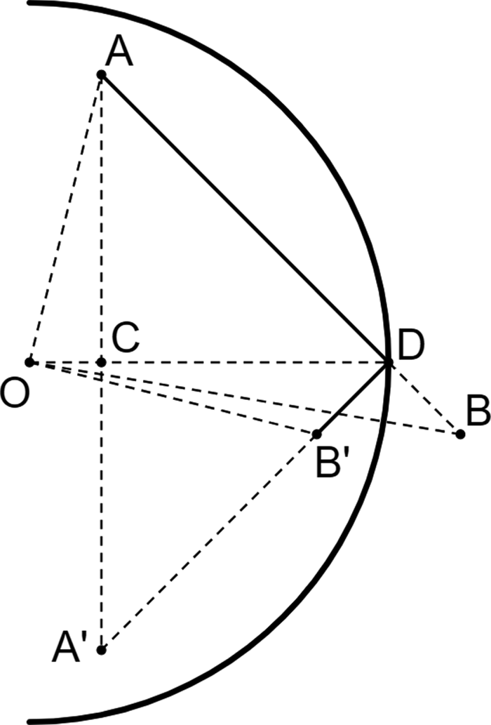
The boundary condition for particles is specular reflection on the surface of the simulation domain, which is straightforward for a cubic simulation domain. For the specular reflection boundary condition on a spherical surface, since no reference is found, we present an implementation that is used in this work, and give its derivation in Appendix A.
Note that the geometry does not matter for the problem studied in this paper. Compared with the cubic domain, the advantage of the spherical domain is that its neutralizing field solution has a much simpler form, but the implementation of the reflection boundary condition on a spherical surface requires the information of particle portions at an old time step.
2.1. Spherical neutralizing field
For a spherical simulation domain, the neutralizing field can be obtained easily from the known analytical solution of the electric field in a uniformly charged sphere centred at the origin (by using a spherical Gaussian surface),

where $\boldsymbol {r}=(x,y,z)$ , $R$
 denotes the radius of the spherical domain. A plot of the field on the $z=0$
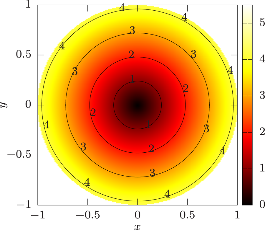
 plane is shown in figure 1.
The magnitude of electric field in a uniformly charged sphere with radius $R$ on the $z=0$
 plane. Values of $R=1$
 , $\rho = 3Q_{\textrm {tot}}/(4 {\rm \pi}R^{3}) = 1$
 and $1/(4 {\rm \pi}\epsilon _0) = 1$
 are used to make the plot.

2.2. Cubic neutralizing field
For a cubic simulation domain, the neutralizing field can be obtained from the electric field in a cube centred at the origin with a size of $2L \times 2L \times 2L$ and a uniformly distributed charge density $\rho =Q_{\textrm {tot}}/(8L^{3})$
 ,

where $\boldsymbol {r}=(x,y,z)$ and $\boldsymbol {r}'=(x',y',z')$
 .
An exact but tedious solution can be obtained by solving the triple integral directly. For the $x$ component, the field reads

where $x_\pm \equiv x \pm L$ , $y_\pm \equiv y \pm L$
 and $z_\pm \equiv z \pm L$
 , $E_y$
 can be obtained by replacing $x$
 with $y$
 , $y$
 with $z$
 and $z$
 with $x$
 ; $E_z$
 can be obtained by replacing $x$
 with $z$
 , $y$
 with $x$
 and $z$
 with $y$
 . The function $F$
 reads

where $t_\pm \equiv \tan [\tan ^{-1}(c_\pm /a)/2]$ . A plot of the field on the $z=0$
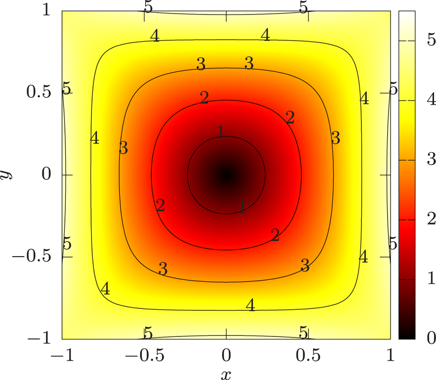
 plane is shown in figure 2. Since no reference is found about this solution, we also provide a brief derivation in Appendix B.
The magnitude of electric field in a uniformly charged cube with length $2L$ on the $z=0$
 plane. Values of $L=1$
 , $\rho = Q_{\textrm {tot}}/(2L)^{3} = 1$
 and $1/(4 {\rm \pi}\epsilon _0) = 1$
 are used to make the plot.

3. Simulation
Since similar PP models have been successfully applied in solving different physical problems (Zhao Reference Zhao2017, Reference Zhao2018a,Reference Zhaoc,Reference Zhaob; Zhao et al. Reference Zhao, Wang and Usui2018), here we only focus on the verification of simulations using like charged particles with the neutralizing fields described in §§ 2.1 and 2.2. To achieve this goal, an electron–ion temperature relaxation problem is chosen, in which electrons and ions are in their own equilibrium but have different temperatures initially, then temperature relaxation occurs due to Coulomb collisions and their temperatures become the same after the relaxation process. For this problem, a theoretical solution is available, as described in § 3.1, with which the PP simulation results can be compared.
All simulations in this work were carried out at the Center for Advanced Research Computing (CARC) at the University of Southern California (https://carc.usc.edu). Decomposition of the particle array is used to parallelize the code with message passing interface (MPI).
3.1. Theoretical solution
Here we consider the commonly used Landau-Spitzer theory, in which the time rate of temperature relaxation reads (Spitzer Reference Spitzer1962; Dimonte & Daligault Reference Dimonte and Daligault2008)

where $\nu _{ei} = \nu _0 \varLambda$ , $\nu _{ie} = (n_e / n_i) \nu _{ei} = Z\nu _{ei}$
 , $\varLambda$
 is the Coulomb logarithm, $Z$
 is the ion charge number, i.e. the number density ratio $n_e / n_i$
 , subscripts $e$
 and $i$
 denote electrons and ions, respectively. The prefactor can be written as (Dimonte & Daligault Reference Dimonte and Daligault2008)

where $e$ is the elementary charge, $k_B$
 is the Boltzmann constant, $m$
 is the particle mass.
Uncertainty arises in choosing the Coulomb logarithm of the form

where $\lambda _D = (\epsilon _0 k_B T_e / n_e e^{2} )^{1/2}$ is the electron Debye length, representing the largest impact parameter before forces are screened out; $R_c = Z e^{2} / 4 {\rm \pi}\varepsilon _0 k_B T_e$
 is the Landau length, representing the smallest impact parameter and characterizing large angle scatterings, which do not occur in weak coupling plasmas. Proposed values of the coefficient $C$
 are found to vary between 1 and 3 under different theoretical approximations (Landau Reference Landau1937; Cohen, Spitzer & Routly Reference Cohen, Spitzer and Routly1950; Thompson & Hubbard Reference Thompson and Hubbard1960; Spitzer Reference Spitzer1962).
In this work, we carry out the simulations under a plasma condition that is chosen by Dimonte & Daligault (Reference Dimonte and Daligault2008), i.e. the non-ideality $\gamma = R_c/\lambda _D = 0.1$ . Under this condition, an implicit solution of the electron temperature $T_e(t)$
 as a function of time $t$
 is (Dimonte & Daligault Reference Dimonte and Daligault2008)

where $\nu _{ei0}$ is calculated using the initial electron and ion temperatures $T_{e0}$
 and $T_{i0}$
 , $\varepsilon = T_{\infty }/T_{e0}$
 , $T_{\infty } = (ZT_{e0}+T_{i0})/(Z+1)$
 denotes the final equilibrium temperature. Then $T_i(t)$
 can be obtained via the relation $T_i = T_{i0} - Z(T_e-T_{e0})$
 . In the following section, simulation results are compared with this theoretical solution.
3.2. Comparison with the theory
For the simulation parameters, we choose electron and ion initial temperatures $T_{e0}=15\ \textrm {eV}$ and $T_{i0}=3\ \textrm {eV}$
 , the number densities $n_e=n_i=9\times 10^{26}\ \textrm {m}^{-3}$
 , i.e. ion charge number $Z=1$
 . These parameters are the same as those in Dimonte & Daligault (Reference Dimonte and Daligault2008) for the case with $\gamma = 0.1$
 . The number of simulated particles are chosen to be $N_e=N_i=8192$
 , such that the domain radius for spherical domain is $R=[3N_e/(4{\rm \pi} n_e)]^{1/3}\approx 12.95\ \textrm {nm}$
 and the domain length for cubic domain is $2L=(N_e/n_e)^{1/3}\approx 20.88\ \textrm {nm}$
 . These parameters lead to a Debye length $\lambda _D \approx 0.96\ \textrm {nm}$
 and an equilibrium temperature $T_\infty = 9\ \textrm {eV}$
 .
Note that, ideally, the periodic boundary condition would be used for studying this problem, but we have found in previous works by Zhao (Reference Zhao2017, Reference Zhao2018a,Reference Zhaob) that if the domain size is sufficiently larger than the Debye length, applying a reflective boundary condition leads to the same relaxation simulation results. For the PP method used in this work, regardless of using like charges or unlike charges, the periodic boundary condition cannot be easily applied. One can refer to the much more computational expensive Ewald summation method (Liu, Hu & Zhao Reference Liu, Hu and Zhao2011) for implementing the periodic boundary condition.
To speed up the simulation, we use an artificial ion mass $m_i/m_e=30$ , which is greater than the minimum mass ratio 25 found in Dimonte & Daligault (Reference Dimonte and Daligault2008) that leads to correct physical results. To apply particles with like charges, both electrons and ions are set to have positive charges. Initially, particle positions are sampled randomly in the corresponding domain, particle velocities are sampled according to Maxwellian distributions based on their temperatures. The time step factor is chosen to be $f_t=0.05$
 . A typical elapsed time for these simulations is 18 hours using 72 MPI ranks running on three CARC nodes, with Intel Xeon E5-2640 v4 processors.
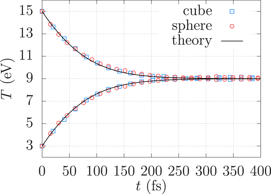
First, the temperature relaxation history of electrons and ions are shown in figure 3. As we can see, due to Coulomb collisions, $T_e$ decreases from 15 eV to 9 eV, and $T_i$
 increases from 3 eV to 9 eV, and the simulation results of both cubic and spherical domain match with the theoretical solution.
Temperature relaxation of simulations in the cubic domain (labelled cube) and in the spherical domain (labelled sphere), and the theoretical solution (labelled theory). The decreasing line and dots are of electrons, the increasing ones are of ions.

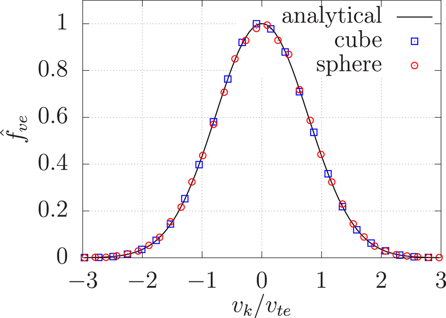
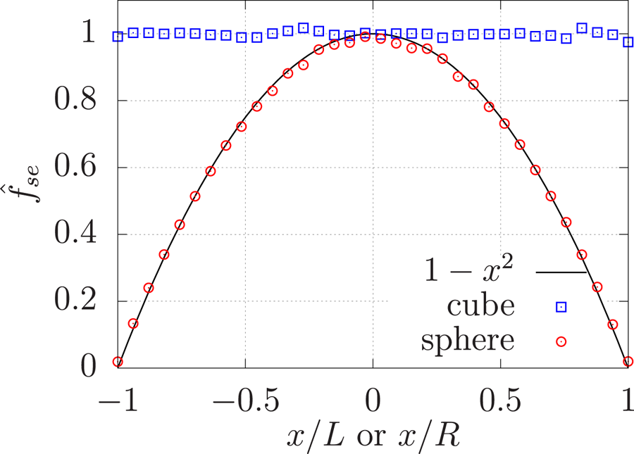
In addition to the correct temperature relaxation, to test the validity of the neutralizing fields, we can also examine the particle velocity distribution function and the particle spatial distribution function, because if the neutralizing fields are wrong, the long-range collective Coulomb forces will not be cancelled, thus the velocity distribution cannot reach the equilibrium easily, and the spatial distribution cannot keep uniform. Therefore, we plot the velocity distribution function of electrons $\,f_{\textrm {ve}}$ as an example at the final equilibrium state in figure 4 to show that the final state is indeed the equilibrium and matches the corresponding Maxwellian distribution. Also, we compute the spatial distribution function of electrons $\,f_{\textrm {se}}$
 along direction $x$
 , i.e. a histogram of the number of electrons in different intervals of $x$
 regardless of $y$
 and $z$
 . For the cubic domain, we should get a constant $\,f_{\textrm {se}}$
 , while for the spherical domain, $\,f_{\textrm {se}}$
 should be proportional to the cross-section area, i.e. $\,f_{\textrm {se}} \propto {\rm \pi}(R^{2}-x^{2})$
 . We found that $\,f_{\textrm {se}}$
 does not vary with time except for small oscillations. We plot the time averaged $\,f_{\textrm {se}}$
 in figure 5.
Normalized electron velocity distribution function $\hat {f}_{\textrm {ve}}$ at the final equilibrium state. Here $\hat {f}_{\textrm {ve}}$
 is averaged over time from 300 to 400 fs and among $x$
 , $y$
 , $z$
 directions to reduce the statistical noise, and its maximum value is normalized to unity. The subscript $k$
 denotes $x$
 , $y$
 or $z$
 , because the plasma is isotropic, the distribution in all directions are the same. Here $v_{te} = (k_B T_{e} / m_e)^{1/2}$
 is the electron thermal velocity. The analytical curve is a Maxwellian distribution for electrons with temperature $T_{e} = 9\ \textrm {eV}$
 .

Normalized electron spatial distribution function $\hat {f}_{\textrm {se}}$ averaged over time from 300 to 400 fs, with the maximum (averaged) value normalized to unity for the spherical (cubic) simulation.

3.3. Comparison with unlike charges
After comparing with the theory, we can further test the validity of the neutralizing fields by comparing with a corresponding simulation using unlike charges. Because simulations using unlike charges have the singularity issue, a cutoff is needed, and it is found that these simulations have worse energy conservation than simulations using like charges. The reason for the worse energy conservation is that, when unlike charges are approaching, their velocities increase due to attraction forces, thus the dynamic time step used should be decreased for accurately solving the trajectories. If the time step is not small enough, two unlike charges could cross each other, which is unphysical but allowed in the simulation (since head-on collisions are rare, and as long as we maintain the energy conservation and confirm that smaller time step does not change the temperature relaxation results anymore). For like charges, their velocities decrease when they are approaching due to repulsive forces, thus it is much easier to solve the trajectories using a relatively bigger time step, and accordingly an easier energy conservation can be achieved. To further speed up the simulations using unlike charges, we choose a smaller mass ratio $m_i/m_e=10$ . Note that although the simulation results may not match the theory anymore due to this small mass ratio, simulations of like and unlike charges should match with each other, and that is our focus in this section.
First, simulations using like charges are carried out with $m_i/m_e=10$ and $f_t=0.1$
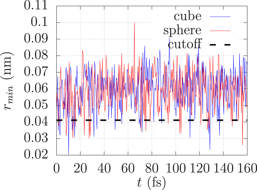
 . Other parameters are the same as those in § 3.2. It is found that the results obtained from these simulations using like charges can help determine the cutoff length for corresponding simulations using unlike charges to avoid the singularity. For example, we can obtain the minimum interparticle distance $r_{\min }$
 at every time step, as shown in figure 6, for both cubic and spherical domains. We could then determine a cutoff length, for example $r_c = 0.041\ \textrm {nm}$
 as indicated by the dashed line in figure 6, which is at least smaller than the majority of $r_{\min }$
 to make sure all necessary interactions are considered. Note that if a chosen cutoff length is not small enough to include all the necessary particle interactions, the temperature relaxation process cannot be correctly captured. One can refer to Zhao (Reference Zhao2017) for more detail about how different cutoff lengths would impact the simulation.
Time history of the minimum interparticle distance.

Then, this cutoff length can be applied to the corresponding simulation using unlike charges. In this work, the cutoff is applied in a way, such that if an interparticle distance is smaller than $r_c$ , the corresponding interparticle force will be ignored. For the corresponding simulation using unlike charges, even if the cutoff $r_c = 0.041\ \textrm {nm}$
 is applied, a smaller time step is required $f_t=0.03$
 to keep the energy conserved within an acceptable range. To further speed up the simulations, we also set a minimum allowed time step $\Delta t = 5.0 \times 10^{-5}\ \textrm {fs}$
 , and the simulated number of particles is reduced to $N_e = N_i = 4096$
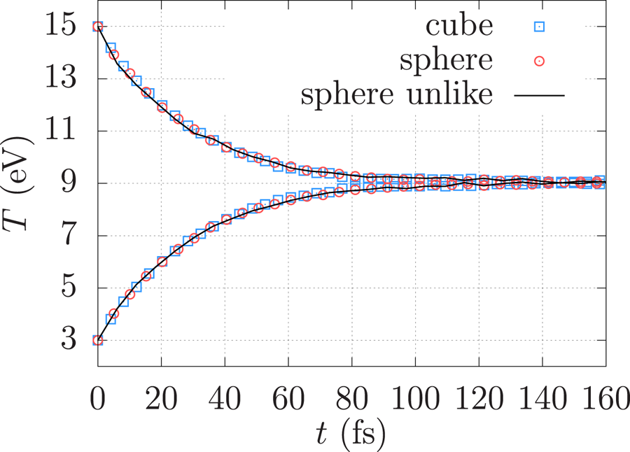
 , as well as the domain size accordingly. Note that as long as the domain size is still large enough compared with the Debye length, the simulation results remain the same, as indicated in previous works (Zhao Reference Zhao2017), because the physics itself is independent of the domain size, theoretically. Here we only consider the spherical domain, as the cubic domain should lead to the same results. The temperature relaxation results of these simulations are shown in figure 7. We can see that the results of using like charges match with those of using unlike charges, as expected.
Temperature relaxation of simulations in the cubic domain (labelled cube) and in the spherical domain (labelled sphere) and a corresponding simulation with unlike charges (labelled sphere unlike).

To study the effects of time step on energy conservation, two more simulations in the spherical domain using like charges are done with $f_t = 0.05$ and $f_t = 1$
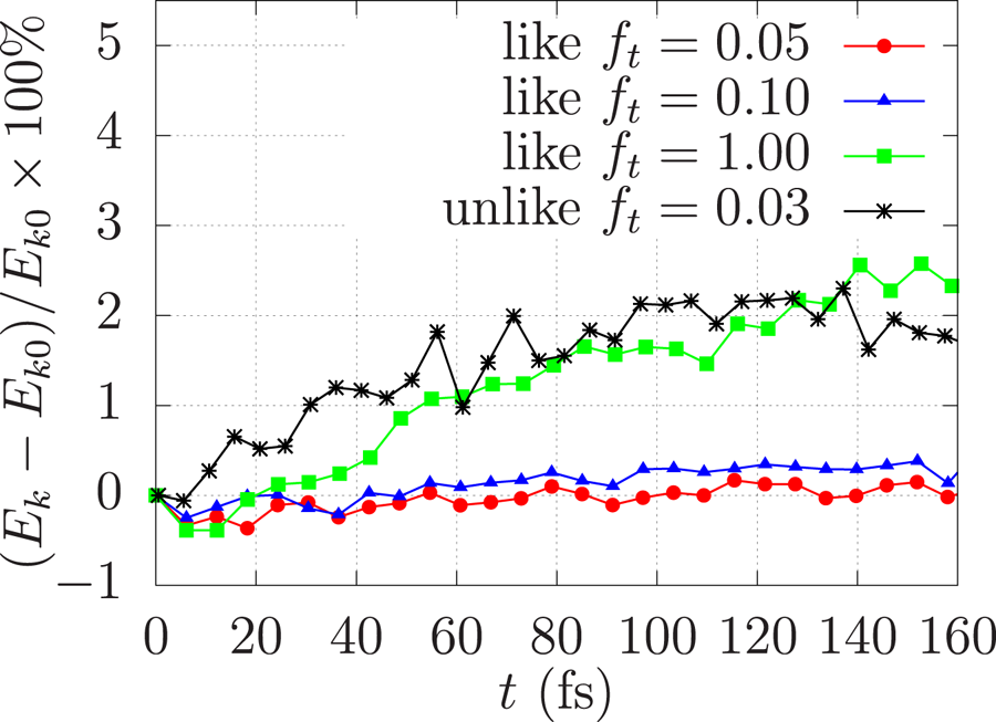
 . Comparing the energy conservations of simulations using like charges, as shown in figure 8, we can see that, a smaller $f_t$
 leads to a better energy conservation. The energy growth is conserved within approximately 0.2 % for $f_t=0.05$
 , 0.6 % for $f_t=0.1$
 and 2.5 % for $f_t=1$
 . For simulations using unlike charges, the energy growth can only be conserved within approximately 2.3 % for $f_t=0.03$
 . Therefore, in addition to the advantage of avoiding the singularity, simulations using like charges have another significant advantage, which is to speed up the simulations. As shown in figure 8, comparing the simulation using like charges with $f_t=1.0$
 with the simulation using unlike charges with $f_t=0.03$
 , we can see a similarity of energy conservation, but the elapsed time of the former is only approximately 0.213 h, and that of the latter is approximately 22 h, when both are using 48 MPI ranks running on two CARC nodes, which indicates a roughly 100 times speed-up. Note that the ratio of the two $f_t$
 used indicates only a 33 times speed-up, the additional three times is due to the different mechanisms of collisions among like charges and unlike charges.
Particle kinetic energy conservation over time.

4. Conclusions and discussions
In this paper, we focus on introducing a way of adding neutralizing fields in PP simulations, such that only like charged particles can be applied to avoid the issue of singularity. We implement the neutralizing fields by applying the analytical solution of the electric field in the domain filled with uniformly distributed charges, for those applications with homogeneous and quasi-neutral plasmas under a reflective boundary condition. The analytical solutions of the neutralizing field in both spherical and cubic domains are considered, between which the spherical solution is simple and known, but the cubic solution has a relatively complicated form and has not been presented in other references, so a brief derivation of the cubic solution is given. Also, one way of implementing the specular reflection boundary condition on a spherical surface is presented. In addition, the approach presented in this work could be generalized for applications with non-homogeneous plasmas, as long as a proper analytical solution of the neutralizing field can be obtained.
To test the validity of the neutralizing fields, simulations on an electron–ion temperature relaxation problem are carried out. The results of the simulations using like charges match the Landau–Spitzer theory and the corresponding simulations using unlike charges. In addition, it is found that using like charges has another significant advantage over using unlike charges besides avoiding the singularity, which is to speed up the simulations by roughly 100 times for the simulations carried out in this work, when keeping the same amount of energy conservation. Also, the simulation results of using like charges can guide simulations using unlike charges, e.g. suggestions can be obtained for choosing a reasonable cutoff length. Note that one may wonder if using like charges is better, why we still need simulations using unlike charges. Simulations using unlike charges could still be beneficial under some circumstances, for example when we intend to set not only a cutoff for the short range, but also one for the long range. In this case, we can only use unlike charges, because the neutralizing fields applied in this paper include all the charges in the domain, thus non-physical results will occur if we apply that long-range cutoff in a simulation using like charges with the neutralizing fields.
At last, it should be mentioned that we do not claim the PP model presented in this paper is a better approach than other PM or PPPM methods that can also solve collisions. However, PP is an alternative method, which can be considered as a first-principle in classical electrostatics, and the results from PP can be used as benchmarks for other methods. For example, one could apply the PP model first on a smaller problem to determine the most appropriate mesh size for a corresponding PPPM model, by finding the minimum effective cutoff length; or for applications with strong particle correlation effects, in which the PP model that solve all PP interactions would be the best choice.
Acknowledgements
The authors acknowledge the Center for Advanced Research Computing (CARC) at the University of Southern California for providing computing resources that have contributed to the research results reported within this publication. Y.H. was partially supported by the LHD Youth Innovation Fund from the State Key Laboratory of High Temperature Gas Dynamics (grant no. LHD2019CX12).
Editor Lus O. Silva thanks the referees for their advice in evaluating this article.
Declaration of interests
The authors report no conflict of interest.
Appendix A. Specular reflection boundary condition on a spherical surface
As illustrated in figure 9, let $O$ denote the centre of the sphere, also the origin of the coordinate system. Assume a particle is located at $A$
 at time $t$
 , thus its position vector is $\boldsymbol {OA}$
 . Assume this particle moves out of the spherical domain, and locates at $B$
 at time $t+\Delta t$
 , thus its position vector is $\boldsymbol {OB}$
 . The plane shown in figure 9 is determined by the two vectors $\boldsymbol {OA}$
 and $\boldsymbol {OB}$
 . Let $\boldsymbol {r}_1 = \boldsymbol {OA}$
 and $\boldsymbol {r}_2 = \boldsymbol {OB}$
 . The relative position vector is then $\boldsymbol {r} = \boldsymbol {r}_2 - \boldsymbol {r}_1 = \boldsymbol {AB}$
 . The distance $\overline {AD}$
 can be obtained according to the line–sphere intersection formula (Eberly Reference Eberly2006),

where $\hat {\boldsymbol {r}} = \boldsymbol {r}/|\boldsymbol {r}| = \boldsymbol {r} / r$ , $R = \overline {OD}$
 is the radius of the sphere. Therefore, $\boldsymbol {AD} = d \hat {\boldsymbol {r}} = \boldsymbol {d}$
 , $\boldsymbol {OD} = \boldsymbol {R} = \boldsymbol {r}_1 + \boldsymbol {d}$
 . Now, $\boldsymbol {DA'}$
 can be obtained by reflecting $\boldsymbol {DA}$
 over $\boldsymbol {OD}$
 ,

where $\hat {\boldsymbol {R}} = \boldsymbol {R}/R$ , $(\boldsymbol {d} \boldsymbol {\cdot } \hat {\boldsymbol {R}})\hat {\boldsymbol {R}} = \boldsymbol {CD}$
 . Thus, the position vector $\boldsymbol {r}'_2$
 after the reflection is

where $\hat {\boldsymbol {d}}' = \boldsymbol {d}' / |\boldsymbol {d}'|$ , $(r-d)\hat {\boldsymbol {d}}' = \boldsymbol {DB'}$
 satisfying $\overline {DB'} = \overline {DB}$
 . If $v_2$
 is the velocity vector at the time $t+\Delta t$
 at the location $B$
 before the reflection, it becomes

after the reflection.
Illustration of the specular reflection boundary condition on a spherical surface.

Appendix B. Derivation of the electric field in a uniformly charged cube
To solve the triple integrals in (2.4), let us only consider the $x$ component first, then change the integrating variables via $u=x-x'$
 , $v=y-y'$
 , $w=z-z'$
 , and integrate once to obtain

where $K\equiv \rho /(4{\rm \pi} \epsilon _0)$ . The inner integral of the first term in (B1) can be solved as

So, (B1) becomes

Steps for solving the integral

are as follows, where $a$ and $b$
 are constants, and $a>|b|$
 , $a>0$
 .
(1) Integrating by parts leads to
(B5)\begin{gather} \int \ln \left(\sqrt{a^{2}+w^{2}}+b\right) \,\textrm{d}w= w \ln\left(\sqrt{w^{2}+a^{2}}+b\right)\nonumber\\ - \int \frac{w^{2}}{\sqrt{w^{2}+a^{2}}\left(\sqrt{w^{2}+a^{2}}+b\right)} \,\textrm{d}w. \end{gather}
(2) Then, the integral in (B5) can be solved by performing trigonometric substitution, $w = a \tan (k)$
, $k = \tan ^{-1}(w/a)$, $\textrm {d}w = a \sec ^{2}(k)\, \textrm {d}k$, and simplifying using $\tan ^{2}(k)+1=\sec ^{2}(k)$,
(B6)\begin{gather} \int \frac{w^{2}}{\sqrt{w^{2}+a^{2}}\left(\sqrt{w^{2}+a^{2}}+b\right)} \,\textrm{d}w \nonumber\\ = a^{2} \int \frac{\sin^{2}(k)}{\cos^{3}(k)} \frac{1}{a/\cos(k) + b} \,\textrm{d} k. \end{gather}(3) Applying Weierstrass substitution with $t = \tan (k/2)$
results in
(B7)\begin{align} \int \frac{\sin^{2}(k)}{\cos^{3}(k)} \frac{1}{a/\cos(k) + b} \,\textrm{d} k ={-}8 \int \frac{t^{2}}{(t-1)^{2}(t+1)^{2}[(b-a)t^{2}-b-a]} \,\textrm{d} t. \end{align}(4) Perform partial fraction decomposition to get
(B8)\begin{gather} \int \frac{t^{2}}{(t-1)^{2}(t+1)^{2}[(b-a)t^{2}-b-a]} \,\textrm{d} t = \int \left( \frac{a^{2}-b^{2}}{4a^{2}[(a-b)t^{2}+a+b]} \right.\nonumber\\ \left.+ \frac{b}{8a^{2}(t+1)}- \frac{1}{8a(t+1)^{2}} - \frac{b}{8a^{2}(t-1)} - \frac{1}{8a(t-1)^{2}} \right)\,\textrm{d} t. \end{gather}(5) The first term in (B8) can be solved by substituting $m=\sqrt {(a-b)/(a+b)}t$
, as follows:
(B9)\begin{equation} \int \frac{1}{(a-b)t^{2}+a+b} \,\textrm{d} t = \frac{\tan^{{-}1}(m)}{\sqrt{a^{2}-b^{2}}}. \end{equation}The other terms in (B8) are simple integrals.





Thus, (B5) becomes

Then (B4) can be expressed by $F(a,b,z)$ given in (2.6). Therefore, we obtain the analytical expressions for the fields as shown in (2.5).