




No CrossRef data available.
Article contents
- Abstract
- 1. INTRODUCTION
- 2. THE GIX/G/1 SYSTEM
- 3. THE GI/R/1 SYSTEM
- 4. THE GIX/R/1 SYSTEM
- 5. APPROXIMATION OF THE GIX/D/1 SYSTEM
- Acknowledgments
- APPENDIX A: An Example with Batch Size Distribution Having Infinite Support
- APPENDIX B: Simple Examples with Batch Size Distribution Having Finite Support
- References
COMPUTATIONAL ANALYSIS OF STATIONARY WAITING-TIME DISTRIBUTIONS OF GIX/R/1 AND GIX/D/1 QUEUES
Published online by Cambridge University Press: 01 January 2005
Article contents
- Abstract
- 1. INTRODUCTION
- 2. THE GIX/G/1 SYSTEM
- 3. THE GI/R/1 SYSTEM
- 4. THE GIX/R/1 SYSTEM
- 5. APPROXIMATION OF THE GIX/D/1 SYSTEM
- Acknowledgments
- APPENDIX A: An Example with Batch Size Distribution Having Infinite Support
- APPENDIX B: Simple Examples with Batch Size Distribution Having Finite Support
- References
Abstract
In this article, we obtain, in a unified way, a closed-form analytic expression, in terms of roots of the so-called characteristic equation of the stationary waiting-time distribution for the GIX/R/1 queue, where R denotes the class of distributions whose Laplace–Stieltjes transforms are rational functions (ratios of a polynomial of degree at most n to a polynomial of degree n). The analysis is not restricted to generalized distributions with phases such as Coxian-n (Cn) but also covers nonphase-type distributions such as deterministic (D). In the latter case, we get approximate results. Numerical results are presented only for (1) the first two moments of waiting time and (2) the probability that waiting time is zero. It is expected that the results obtained from the present study should prove to be useful not only for practitioners but also for queuing theorists who would like to test the accuracies of inequalities, bounds, or approximations.
Information
- Type
- Research Article
- Information
- Probability in the Engineering and Informational Sciences , Volume 19 , Issue 1 , January 2005 , pp. 121 - 140
- Copyright
- © 2005 Cambridge University Press
1. INTRODUCTION
Consider the queuing system GIX/G/1, where groups of customers of random size X arrive at the system following a renewal process and are served by a single server with a general service-time distribution. The group size has a known distribution: Pr(X = i) = gi (i = 0,1,…; g0 ≡ 0) with finite mean and squared coefficient of variation (SCV), mg and cg2, respectively. The interbatch-time (service-time) distribution function is denoted by A(x) (B(x)) and has finite mean λ−1 (μ−1) and SCV ca2 (cs2). The interbatch times, the service times, and the group sizes are mutually independent. The queue discipline is first-in first-out (FIFO) with respect to the groups; the order within a group is random and the service is individual. Since we consider the equilibrium behavior of the queue, the traffic intensity ρ = λmg /μ < 1.
The need to determine the stationary waiting-time distribution for the GIX/G/1 queue is well recognized. This is attributed to its importance in the area of communication, transportation, and manufacturing systems. However, substantial difficulties existed in the computation of the stationary waiting-time distribution either by an analytical or by a numerical approach. These difficulties have been alleviated by the introduction of an R-type distribution, where R denotes a class of distributions whose Laplace–Stieltjes transforms (LSTs) are rational functions (ratios of a polynomial of degree at most n to a polynomial of degree n). The consideration of the distributions belonging to class R is not a great restriction since, in practice, almost any distribution can be approximated by a distribution belonging to this class; see Chaudhry, Agarwal, and Templeton [4] (discussed later in Section 2). It is interesting to note that the stationary waiting-time distribution of an arbitrary customer in a group is the sum of two independent random variables (r.v.'s), one of which can be expressed explicitly in terms of the given parameters, whereas the other, namely the waiting time of the customer who is the first to receive service in a group, is equal to the delay in the “dual” queue GI/GX /1, where the service time is a sum of a random number (X) of independent and identically distributed (i.i.d.) r.v.'s and, hence, Gx represents the convolution of X service times. Therefore, the study of the GIX/G/1 queue can be reduced to the study of the GI/GX /1 queue, the latter being a special class of the GI/G/1 queue.
In this article, we first present a simple known result of the LST of the stationary waiting-time distribution of the GIX/G/1 queue, which was analyzed by Yao, Chaudhry, and Templeton [11]. Then, following Chaudhry et al. [4], we express the stationary waiting-time distribution of the GIX/R/1 queue in terms of roots of the so-called characteristic equation (c.e.). It may, however, be remarked that whereas Yao et al. [11] consider only approximate results for the mean waiting time, we give a complete distribution, in terms of roots, both analytically and computationally at least for the GIX/R/1 queue. It may be further remarked that even the transcendental or irrational functions for service times can be handled by the procedure given here. This is exemplified by considering the GIX/D/1 model, which is otherwise difficult to solve, although it is very useful in telecommunications systems. Furthermore, our procedure works for both finite and specialized infinite support group size distributions such as geometric. The numerical experiments have also been carried out and some of these results are included in various self-explanatory tables. Since it is instructive to explain the procedure by simple examples, this is done both for the special cases of the GIX/R/1 and GIX/D/1 queues and the results are presented in Appendix B.
The rest of the article is organized as follows. In Section 2, the LST of the stationary waiting-time distribution of the GIX/G/1 queue given in Yao et al. [11] is repeated. In Section 3, we present the stationary waiting-time distribution of the GI/R/1 queue derived in Chaudhry et al. [4]. In Section 4, we derive the stationary waiting-time distribution of the GIX/R/1 queue and provide some numerical results. In Section 5, we get approximate results for the GIX/D/1 queue and provide some numerical examples.
2. THE GIX/G/1 SYSTEM
Let Wq*(s) be the LST of the stationary waiting-time distribution of an arbitrary customer in a group at an arrival epoch. The following notation (see [11]) is used. (Since we consider the equilibrium behavior of the queue, the traffic intensity ρ = λmg /μ < 1.)

Proposition 1 [11]:

where Wq1*(s) is the LST of the (stationary) waiting time of the customer who is the first to receive service in a group. This is equal to the LST of the waiting time in the GI/GX /1 queue, where the service time is a sum of a random number (X) of i.i.d. r.v.'s. Wq2*(s) is the LST of an additional (stationary) waiting time for the random customer of a group,

3. THE GI/R/1 SYSTEM
Let us assume that

where P(s) is a polynomial of degree at most n and Q(s) is of degree n. We further assume that P(s) and Q(s) have no common factors, and let

respectively be the LST of the interbatch-time and service-time distributions for the GI/R/1 queue. Assumption (3.1) does not amount to any great limitations on the scope of the analysis of the GI/G/1 queue, as this class can fit almost all of the distributions that may arise in practice, as noted by several researchers; see, for example, Botta, Harris, and Marchal [2]. Further, Bladt [1] shows that there is a one-to-one correspondence between matrix-exponential distributions and distributions having rational Laplace transforms. Examples are given by Bladt [1] and Botta et al. [2] to show that even distributions that cannot be represented by phase type (PH) belong to a somewhat smaller class than the matrix-exponential. Such examples that do not belong to PH distributions can also be handled by our method. In view of this, it is worth emphasizing that the method of rational transforms discussed in this article is not only more comprehensive than the phase method, but it is also computationally more efficient, although the former may not have a direct probabilistic interpretation. We assume that the coefficient of sn in Q(s) is unity and denote the same in P(s) by an, which satisfies the relation |an| ≤ 1 (see [4, Thm.1]). Although (3.2)–(3.9) are given in Chaudhry et al. [4], they are repeated here for easy readability of the article.
Denoting by Wq*(s) the LST of Wq(t), the cumulative distribution function (CDF) of the stationary waiting time, it follows from (3.3) of [4, p.112] that

where Wq−*(s) is the LST of Wq−(t) defined by

and

Using spectrum factorization (Kleinrock [7, pp.286,287,288,289,290]), we have from (3.4) of [4, p.112] that

where si (i = 1,2,…,n) are the roots (assumed distinct) of the c.e.,

, with Re(si) < 0.
Resolving (3.5) into partial fractions, we get

where

Also, the probability density function (pdf) wq(t) and the CDF Wq(t) of the waiting time are obtained as

and

where δ(t) is the Dirac delta function.
4. THE GIX/R/1 SYSTEM
Let us assume that

where P(s) and Q(s) are the same as in (3.1). We consider the case with batch size distribution having finite support: Pr(X = i) = gi,i = 1,2,…,k. We now consider the functions Wq1*(s), Wq2*(s), and Wq*(s) under three separate cases: (4.1), (4.2), and (4.3), respectively.
Case 4.1: Wq1*(s)
Denoting by

the LST of the service-time distribution in the GI/GX /1 queue, we have

where

Remarks:
- U(s) is a polynomial of degree at most nk and V(s) is of degree nk.
- U(s) and V(s) have no common factors.
- The coefficient of snk in
V(s) is unity and the same in U(s)
is unk, where
satisfies the relation |unk| ≤ 1. Note that |unk| ≤ 1 is a condition that is needed in Theorem 1 of [4].

From (3.6) and (3.7), we get

where si (i = 1,2,…,nk) are the roots (assumed distinct) of the c.e.,

, with Re(si) < 0,

They satisfy the relation

Case 4.2: Wq2*(s)
From (2.2), we obtain Wq2*(s) as

where

Remarks:
- C(s) is a polynomial of degree less than n(k − 1) and D(s) is of degree n(k − 1).
- Since we assume that P(s) and Q(s) have no common factors, C(s) and D(s) have no common factors.
- Since Wq2*(s) is convergent for Re(s) ≥ 0, D(s) has no zeros in Re(s) ≥ 0. This implies that it has zeros in the open half-region Re(s) < 0, say xi (i = 1,2,…,n), (assumed distinct) where xi has a multiplicity of k − 1.
Resolving (4.7) into partial fractions (see [6, pp.24,25,26]), we obtain

where

They satisfy the relation

Case 4.3: Wq*(s)
Using (4.4) and (4.9), we rewrite (2.1) as

For further analysis, let us assume that

have no common zeros (see Theorem 1 of Chaudhry et al. [4]). Then, all si and xj are distinct roots. Otherwise, minor modifications are needed and can be easily dealt with, as we have done in Remark (3) of Case 4.2.
Taking the inverse LST of (4.12), explicit closed-form expressions of the pdf wq(t) and the CDF Wq(t) of the stationary waiting time of a customer are found to be

and

where

From (4.14) and (4.6), we obtain the (stationary) probability of no wait in queue as

Using (4.6), (4.11), and (4.12), we get the following expression for the first moment, E(Wq):

for the second moment, E(Wq2), we obtain

The expressions for the stationary waiting-time distribution of the GIX/R/1 queue and its first two moments are obtained as above. The presented results have a definite value for the practical engineers and are also useful for the queuing theorists to test the accuracies of inequalities, bounds, or approximations. We now provide some numerical examples.
Numerical Examples
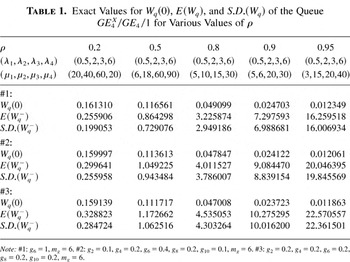
Although complete distributions can be obtained, we only give a few performance measures in a self-explanatory table (Table 1). Consider the GE4X/GE4 /1 queue. In this case, we take

. Then, using the procedure described in this section, we carry out numerical work for several cases. From (4.15), (4.16), and (4.17), we present sample numerical results for Wq(0), E(Wq), and S.D.(Wq).
Exact Values for Wq(0), E(Wq), and S.D.(Wq) of the Queue GE4X/GE4 /1 for Various Values of ρ

5. APPROXIMATION OF THE GIX/D/1 SYSTEM
In this section, we consider the GIX/D/1 queue, where each customer arriving in a group requires a deterministic service time that could be greater than or equal to one (i.e., D ≥ 1). This queuing model has gained importance in recent years in view of a number of possible practical applications to telecommunications systems. It may be possible to find explicit results for the (stationary) waiting time of the GIX/D/1 queue, but the results are likely to be very complex, as can be seen from the results of the GI/D/1 queue discussed by Chaudhry [3]. However, it is much better to use continued fractions, as they give good approximate results with much simplified algebra. Although the procedure being discussed here is more general because it covers transcendental and irrational functions, it is exemplified by considering only the exponential function. Continued fractions are quite useful in computation, as they usually provide representations for transcendental functions that are much more generally valid than the classical representation by power series (see, e.g., Parthasarathy and Balakrishnan [8] for another use of continued fractions). In this article, we make use of the continued fractions approach to approximate the exponential function, and then approximate results for the GIX/D/1 queue.
5.1. Continued-Fractions Representation for Exponential Function
Exponential function ez can be represented in the form of continued fractions as follows (see [9]):

which is valid for all z ∈ C.
Using (2.14) of Cooper and Thron [5, p.235], the even part of (5.1) is defined by

Let An (Bn) denote the nth numerator (denominator) and let fn denote the nth approximant of (5.2) (i.e., 2nth approximant of (5.1)). Then, these are defined as

where

and

Remark: Note that fn = An /Bn is a rational function of complex variable z (ratios of a polynomial of degree n − 1 to a polynomial of degree n).
5.2. Approximation by the Continued Fractions
Confining ourselves to the GIX/D/1 queue, we have

if the service time is constant and equal to 1/μ.
Replacing z by −s/μ in (5.2) gives the representation

Denoting by Pn(s) (Qn(s)) the nth numerator (denominator) and letting

denote the nth approximant of (5.2), we have

where

and

It may be remarked here that

is a rational function where the numerator (Pn(s)) is a polynomial of degree n − 1 and the denominator (Qn(s)) is a polynomial of degree n; that is,

can be approximated by the R-type distribution mentioned in the previous section. As a consequence, we can approximate the GIX/D/1 queue using the results of the GIX/R/1 queue studied in Section 4, and, thus, we will omit the details in this section. We demonstrate the performance of our approximations in the tables.
Numerical Examples
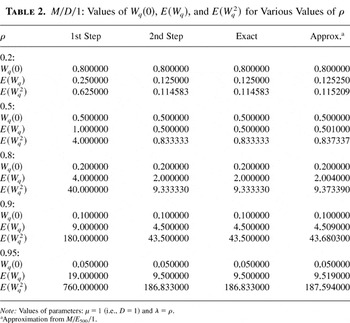
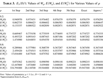
In order to examine the performance of our approximations, some calculations for the numerical computations of Wq(0), E(Wq), and E(Wq2) were done for the MX/D/1 and E3X/D/1 queues, which are special cases of GIX/D/1.
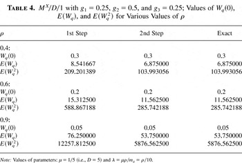
Tables 2 and 3 contain the results for M/D/1 and E3 /D/1, respectively, for various values of ρ. These values have been selected for illustrative purposes, but the method puts no restrictions on any reasonable value of ρ. We take the exact and approximate values from Chaudhry [3]. It may be remarked that the time taken to get the results of M/E500 /1 and E3 /E500 /1 is more than that of getting the results of M/D/1 and E3 /D/1 by continued fractions, as the number of roots required is 500 in the former case. In addition, Tables 4 and 5 give results for MX/D/1 with g1 = 0.25, g2 = 0.5, and g3 = 0.25 and E32/D/1, respectively. The exact values are obtained from Takagi [10, pp.46,47] and Chaudhry [3], respectively, since the waiting-time distribution of E32/D/1 is equivalent to that of E3 /D2 /1, where D2 is convolution of D with itself.
M/D/1: Values of Wq(0), E(Wq), and E(Wq2) for Various Values of ρ

E3 /D/1: Values of Wq, E(Wq), and E(Wq2) for Various Values of ρ

MX/D/1 with g1 = 0.25, g2 = 0.5, and g3 = 0.25; Values of Wq(0), E(Wq), and E(Wq2) for Various Values of ρ

E32/D/1: Values of Wq(0), E(Wq), and E(Wq2) for Various Values of ρ

It can be seen from Tables 2, 3, 4, and 5 that as the number of steps (n) increases, the performance of approximation increases and the approximate value converges rapidly into the exact value. The steps are defined at the end of Table 5.
We hope that our approximation would be beneficial for practitioners who would like practical answers to their bulk-arrival queuing systems with deterministic service time.
We approximate

as follows:

Acknowledgments
The first author acknowledges with thanks the partial financial support (from BK 21 project) and other facilities provided by the Department of Industrial Engineering, KAIST, where he held invited distinguished professorship. This research was also supported (in part) by NSERC.
APPENDIX A: An Example with Batch Size Distribution Having Infinite Support
It is interesting to note that if we assume geometric batch size, the results, as expected, become much simpler. This is illustrated here.
Suppose the group size X has a geometric distribution:

where q = 1 − p, 0 < p < 1, and n = 1,2,….
In this case,

, which is a rational function. Following the procedure described in Section 4, we get from (4.4),

where si (i = 1,2,…,n) are the roots (assumed distinct) of the c.e.,

, with Re(si) < 0, where

and

Also, we have from (4.9),

where

and xi (i = 1,2,…,n) are the roots (assumed distinct) of the c.e., D(s) = 0, with Re(xi) < 0, where

Using (A.1) and (A.4), we get

Taking the inverse LST of (A1.7), explicit closed-form expressions of the pdf wq(t) and the CDF Wq(t) of the waiting time of a customer are found to be (assuming all roots are distinct)

and

Remark. As a further check, note that limt→∞ Wq(t) → 1, as it should, if we use (A.4).
From (A.9) and (A.1), we obtain the probability of no wait in queue as

From (A.7) and (A.1) and (A.4) with s = 0, we get the first moment, E(Wq), as

and the second moment, E(Wq2), as

APPENDIX B: Simple Examples with Batch Size Distribution Having Finite Support
Case 1: An Example of the GIX/R/1 Queue
We consider the queue M3/M/1. In this case, from (4.4) and (4.5), we get

where si (i = 1,2,3) are the roots of the c.e., [λ/(−s + λ)]μ3 − (s + μ)3 = 0, with Re(si) < 0 and

From (4.9) and (4.10), we have

where

Further, from (4.16), we get the following expression for E(Wq):

From (4.17), we have

Finally, we have from (4.14) that

Case 2: An Example of the GIX/D/1 Queue
We consider the queue M2/D/1. From (5.8), we can approximate

as follows (see approximation steps given in numerical examples of Section 5.2):

From (4.4) and (4.5), we get

where

and

are the roots of the c.e., [λ/(−s + λ)]μ2 − (s + μ)2 = 0, with Re(si) < 0 and

From (4.9) and (4.10), we have

where

Further, from (4.16), we get the following expression for E(Wq):

from (4.17), we have

Finally, we have from (4.14) that

References
REFERENCES
Bladt, M.
(1993).
Ph.D. thesis,
Aalborg University, Denmark.
Botta, R.F.,
Harris, C.M., &
Marchal, W.G.
(1987).
Characterization of generalized hyperexponential distribution
functions.
Communications in Statistics: Stochastic Models
3:
115–148.Google Scholar
Chaudhry, M.L.
(1992).
Computing stationary queueing-time distributions of GI/D/1
and GI/D/c queues.
Naval Research Logistics
39:
975–996.Google Scholar
Chaudhry, M.L.,
Agarwal, M., &
Templeton, J.G.C.
(1992).
Exact and approximate numerical solutions of steady-state
distributions arising in the queue GI/G/1.
Queueing Systems
10:
105–152.Google Scholar
Cooper, S.C. &
Thron, W.J.
(1994).
Continued fractions and orthogonal functions: Theory and
applications.
New York:
Marcel Dekker.
Giffin, W.C.
(1975).
Transform techniques for probability modeling.
New York:
Academic Press.
Kleinrock, L.
(1975).
Queueing systems.
Vol. 1.
New York:
Wiley,
Parthasarathy, P.R. &
Balakrishnan, N.
(1990).
A continued fraction approximation of the modified Bessel function
I(t).
Applied Mathematics Letter
3:
13–15.Google Scholar
Staff of Research and Education Association.
(1992).
Handbook of mathematical, science, and engineering formulas,
tables, functions, graphs, transforms.
New York:
Research & Education Association.
Takagi, H.
(1991).
Queueing analysis,
Vol. 1.
Amsterdam:
North-Holland.
Yao, D.D.
Chaudhry, M.L., &
Templeton, J.G.C.
(1984).
Analyzing the steady-state queue GIX/G/1.
Journal of the Operational Research Society
35:
1027–1030.Google Scholar
Exact Values for Wq(0), E(Wq), and S.D.(Wq) of the Queue GE4X/GE4 /1 for Various Values of ρ
M/D/1: Values of Wq(0), E(Wq), and E(Wq2) for Various Values of ρ
E3 /D/1: Values of Wq, E(Wq), and E(Wq2) for Various Values of ρ
MX/D/1 with g1 = 0.25, g2 = 0.5, and g3 = 0.25; Values of Wq(0), E(Wq), and E(Wq2) for Various Values of ρ
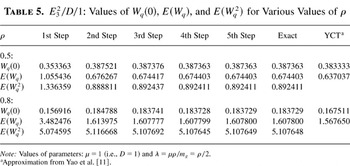
E32/D/1: Values of Wq(0), E(Wq), and E(Wq2) for Various Values of ρ
 You have
Access
- 4
- Cited by